The classical origin of quantum affine algebra in squashed sigma models

Abstract

We consider a quantum affine algebra realized in two-dimensional non-linear sigma models with target space three-dimensional squashed sphere. Its affine generators are explicitly constructed and the Poisson brackets are computed. The defining relations of quantum affine algebra in the sense of the Drinfeld first realization are satisfied at classical level. The relation to the Drinfeld second realization is also discussed including higher conserved charges. Finally we comment on a semiclassical limit of quantum affine algebra at quantum level.

1 Introduction

Integrable quantum field theories are wonderful laboratories to develop non-perturbative methods such as strong/weak-coupling dualities. Some examples are principal chiral models and $O(N)$-invariant non-linear sigma models, and these are integrable at both classical and quantum mechanical level Luscher1 ; Luscher2 . The integrability is closely related to the symmetric coset structure of target space AAR .

For symmetric coset target spaces, a general prescription to construct an infinite number of classical conserved charges is well known Luscher2 ; AAR ; BIZZ and the charges obtained along it form the Yangian algebra Bernard-Yangian ; MacKay , mathematically formulated by Drinfeld Drinfeld . Then the quantum integrability can be argued by checking whether the conservation laws of the charges are anomalous or not GW ; AFG . When the system is quantum mechanically integrable, the Bethe ansatz technique works well as in principal chiral models PW .

The integrability plays an important role in the recent study of AdS/CFT Maldacena (For a comprehensive review see review ). In particular, the classical integrability of sigma model on the string theory side is discussed in BPR and it is inherited from the behind structure of AdS/CFT, the parent integrable spin chain. It would be a nice direction to seek for a generalization of AdS/CFT preserving the sigma model integrability. Within a class of symmetric spaces including the supersymmetric extension, it has been done quite generally in Zarembo . Hence the next is to consider non-symmetric cosets as a generalization.

There are some integrable deformations of AdS/CFT, for example, $\beta$-deformation LS ; LM ; Frolov ; Berenstein and $q$-deformation of the world-sheet S-matrix BK ; BGM ; Hollowood . However, we are interested in another class of integrable deformations concerning warped AdS spaces and squashed spheres in three dimensions, which are represented by non-symmetric cosets. Since warped AdS spaces are obtained via double Wick rotations from squashed spheres, we are confined to squashed spheres here. The main subject in this paper is to gain more insight into the classical integrable structure of two-dimensional non-linear sigma models with squashed spheres as target space.

Although the squashed sigma models are well known as an integrable model of the trigonometric class, it has been shown that a Yangian symmetry $Y(sl(2))$ is realized even after the squashing in a series of works KY ; KOY ; KYhybrid (For a short summary see KY-summary ). This result may sound curious. However, in fact, there exist two descriptions to describe the classical dynamics, i) the trigonometric description and ii) the rational description. That is, it is possible to construct two types of Lax pair, both of which lead to the identical classical equations of motion. The two descriptions are related to each other via a non-local map. Furthermore, a finite-dimensional quantum group symmetry $U_{q}(sl(2))$ Drinfeld ; Jimbo is realized at classical level in terms of non-local currents corresponding to the broken generators due to the squashing of target space. This is nothing but a classical origin of quantum group symmetry Drinfeld ; Jimbo . The explicit relation between the algebraic deformation parameter $q$ of the quantum group $U_{q}(sl(2))$ and the geometric deformation parameter of squashed three sphere is also given by KYhybrid .

In this paper, as a generalization of the previous result, it is shown that the quantum group symmetry $U_{q}(sl(2))$ is enhanced to the quantum affine algebra $U_{q}(\widehat{sl(2)})$ at classical level. An infinite number of classical conserved charges are derived by expanding the monodromy matrix constructed with the Lax pair in the trigonometric description FR . The infinite tower structure of the charges with the Poisson bracket turns out to be a classical analogue of quantum affine algebra $U_{q}(\widehat{sl(2)})$ Drinfeld . Firstly, we show that the Poisson brackets of the level $0,\pm 1$ charges satisfy the defining relations of the quantum affine algebra $U_{q}(\widehat{sl(2)})$ in the sense of the Drinfeld first realization. Secondly, we argue that including all of the higher charges recast the tower structure into the Drinfeld second realization.

This paper is organized as follows. In section 2 we introduce the classical action of squashed sigma models and the monodromy matrix in the trigonometric description. In section 3 an infinite set of conserved (non-local) charges are derived by expanding the monodromy matrix. In section 4, by evaluating the classical Poisson brackets, we show that they actually coincide with the defining relations of quantum affine algebra $U_{q}(\widehat{sl(2)})$ in the sense of the Drinfeld first realization. Then we argue the relation between higher conserved charges and the Drinfeld second realization at classical level. In section 5 we comment on a semiclassical limit of quantum affine algebra realized at quantum level. Section 6 is devoted to conclusion and discussion. In Appendix A we give a proof of the classical $q$-Serre relations, which are a part of the defining relations in the Drinfeld first realization and impose constraints on the higher conserved charges.

2 Squashed sigma model and monodromy matrix

We consider two-dimensional non-linear sigma models with target space squashed sphere in three dimensions. The classical action is given by

$$S[J] = \!\!\int\!\!\!\!\int\!\!dtdx\Bigl{[}{\rm Tr}\left(J_{\mu}J^{\mu}\right)-2C\,{\rm Tr}\!\left(T^{3}J_{\mu}\right)\!{\rm Tr}\!\left(T^{3}J^{\mu}\right)\Bigr{]}\,,$$ (1)

$$J_{\mu}\equiv g^{-1}\partial_{\mu}g\,,\qquad g\in SU(2)\,.$$

The coordinates and metric of base space are $x^{\mu}=(t,x)$ and $\eta_{\mu\nu}={\rm diag}(-1,+1)$ . Suppose that the value of $C\in\mathbb{R}$ is restricted to $C>-1$ so that the sign of kinetic term is not flipped. The $SU(2)$ Lie algebra generators $T^{a}~{}(a=1,2,3)$ satisfy

$$[T^{a},T^{b}]=\varepsilon^{ab}_{~{}~{}c}T^{c}\,,\qquad{\rm Tr}(T^{a}T^{b})=-\frac{1}{2}\delta^{ab}\,,$$ (2)

where $\varepsilon^{ab}_{~{}~{}c}$ is the totally anti-symmetric tensor.

This system has the $SU(2)_{\rm L}\times U(1)_{\rm R}$ symmetry. The non-zero value of $C$ breaks the original $SU(2)_{\rm L}\times SU(2)_{\rm R}$ symmetry of round $S^{3}$ to $SU(2)_{\rm L}\times U(1)_{\rm R}$ . As a matter of course, the $SU(2)_{\rm L}\times SU(2)_{\rm R}$ symmetry recovers when $C=0$ .

Note that the Virasoro and periodic boundary conditions are not imposed here, though we have some applications in string theory in our mind. Instead of them, we impose the boundary condition that the group variable $g(x)$ approaches a constant element rapidly as it goes to spatial infinity like

$$g(x)\to g_{\infty}~{}:~{}\mbox{const.}\qquad(x\to\pm\infty)\,.$$ (3)

That is, $J_{\mu}(x)$ vanishes rapidly as $x\to\pm\infty$ .

The classical equations of motion are obtained in the usual manner as

$$\partial^{\mu}J_{\mu}-2C{\rm Tr}(T^{3}\partial^{\mu}J_{\mu})T^{3}-2C\,{\rm Tr}(T^{3}J_{\mu})[J^{\mu},T^{3}]=0\,.$$ (4)

It is possible to construct two types of Lax pair which lead to the identical equations of motion (4) and these are equivalent through a non-local map KYhybrid . That is, there are two equivalent ways in describing the classical dynamics, 1) the rational description based on $SU(2)_{\rm L}$ and 2) the trigonometric description based on $U(1)_{\rm R}$ .

We work below in the trigonometric description, where the Lax pair is given by FR

$$L^{R}_{t}(x;\lambda) = \sum_{a=1}^{3}\left[w_{a}(\lambda+\alpha)S^{a}-w_{a}(\lambda-\alpha)\bar{S}^{a}\right]T^{a}\,,$$

$$L^{R}_{x}(x;\lambda) = \sum_{a=1}^{3}\left[w_{a}(\lambda+\alpha)S^{a}+w_{a}(\lambda-\alpha)\bar{S}^{a}\right]T^{a}\,.$$ (5)

Here $\lambda\in\mathbb{C}$ is a spectral parameter and $w_{a}(\lambda)$ is defined as

$$w_{1}(\lambda)=w_{2}(\lambda)\equiv\frac{1}{\sinh\lambda}\,,\qquad w_{3}(\lambda)\equiv\coth\lambda\,.$$ (6)

Then $S^{a}$ and $\bar{S}^{a}$ are related to $J_{\mu}^{a}\equiv-2{\rm Tr}(T^{a}J_{\mu})$ like

$$J_{t}^{3}=(w_{1}(2\alpha)+w_{3}(2\alpha))(S^{3}+\bar{S}^{3})\,,$$

$$J_{x}^{3}=(w_{1}(2\alpha)+w_{3}(2\alpha))(S^{3}-\bar{S}^{3})\,,$$

$$J_{t}^{1,2}=\sqrt{2w_{1}(2\alpha)(w_{1}(2\alpha)+w_{3}(2\alpha))}\,(S^{1,2}+\bar{S}^{1,2})\,,$$

$$J_{x}^{1,2}=\sqrt{2w_{1}(2\alpha)(w_{1}(2\alpha)+w_{3}(2\alpha))}\,(S^{1,2}-\bar{S}^{1,2})\,,$$

and the parameter $\alpha$ is written in terms of the squashing parameter $C$ as

$$\cosh\alpha\equiv\frac{1}{\sqrt{1+C}}\,,\qquad\sinh\alpha\equiv\frac{i\sqrt{C}}{\sqrt{1+C}}\,.$$

Note that $\alpha$ is pure imaginary for $C>0$ and real for $C<0$ . When $C=0$ , $\alpha=0$ .

The commutator

$$[\partial_{t}+L_{t}^{R}(x;\lambda),\partial_{x}+L_{x}^{R}(x;\lambda)]=0$$

leads to the equations of motion in (4) as well as the Maurer-Cartan equation

$$dJ+J\wedge J=0\,.$$

Then the monodromy matrix $U^{R}(\lambda)$ is defined as

$$U^{R}(\lambda) \equiv {\rm P}\exp\left[-\int^{\infty}_{-\infty}\!\!\!dx\,L^{R}_{x}(x;\lambda)\right]\,.$$ (7)

It is straightforward to show that this is a conserved quantity,

$$\frac{d}{dt}U^{R}(\lambda)=0\,.$$

It would be helpful later to use the following form of $L^{R}_{x}(x;\lambda)$ ,

$$L^{R}_{x}(x;\lambda) = \frac{\sinh\alpha}{\sinh(\lambda-\alpha)\sinh(\lambda+\alpha)}\biggl{[}T_{3}\left(\frac{\sinh\lambda\cosh\lambda}{\cosh\alpha}J^{3}_{t}(x)-\sinh\alpha J^{3}_{x}(x)\right)$$

$$+\left.T_{+}\left(\cosh\alpha\sinh\lambda J^{+}_{t}(x)-\sinh\alpha\cosh\lambda J^{+}_{x}(x)\right)\right.$$

$$+T_{-}\left(\cosh\alpha\sinh\lambda J^{-}_{t}(x)-\sinh\alpha\cosh\lambda J^{-}_{x}(x)\right)\biggr{]}\,,$$

where we have introduced the following notations,

$$T^{\pm}\equiv\frac{1}{\sqrt{2}}(T^{1}\pm iT^{2})=T_{\mp}\,.$$

An infinite number of conserved charges are obtained by expanding the monodromy matrix $U^{R}(\lambda)$ with respect to $\lambda$ around an expansion point. The expression of charges depends on expansion points.

3 Expanding monodromy matrix

Let us expand the monodromy matrix $U^{R}(\lambda)$ with the complex parameter $z=e^{-\lambda}$. Depending on the regions of the complex plane, we obtain the following two expansions

$$\mbox{i)}\qquad U^{R}(\lambda) =e^{\bar{u}_{0}}\exp\left[\sum_{n=1}^{\infty}z^{n}\bar{u}_{n}\right]\qquad{\rm for}\quad|z|<1\quad{\rm(or}\quad{\rm Re}(\lambda)>0)$$ (8)

$$\mbox{ii)}\qquad U^{R}(\lambda) =e^{u_{0}}\exp\left[\sum_{n=1}^{\infty}z^{-n}u_{n}\right]\qquad{\rm for}\quad|z|>1\quad{\rm(or}\quad{\rm Re}(\lambda)<0)$$ (9)

Corresponding the expanding coefficients $\bar{u}_{0}$, $\bar{u}_{n}$ and $u_{0}$, $u_{n}$ ($n\geq 1$), we would define the conserved charges $\bar{Q}^{R,a}_{(n)}$ and $Q^{R,a}_{(n)}$ respectively, where superscript $a$ runs $\pm,3$ and denotes the triplet generators of $sl(2)$ . An infinite number of conserved non-local charges are obtained systematically at classical level. These charges are nothing but the generators of quantum affine algebra $U_{q}(\widehat{sl(2)})$ as we will discuss later.

3.1 Expansion i)

Let us consider the expansion i). Then the spatial component of the Lax pair is expanded around $z=0$ like

$$L^{R}_{x}(x;\lambda) = i\sqrt{C}T_{3}J^{3}_{t}(x)$$

$$+z\left[T_{+}\left(\frac{2i\sqrt{C}}{1+C}J^{+}_{t}(x)+\frac{2C}{1+C}J^{+}_{x}(x)\right)\right.$$

$$\left.\qquad+T_{-}\left(\frac{2i\sqrt{C}}{1+C}J^{-}_{t}(x)+\frac{2C}{1+C}J^{-}_{x}(x)\right)\right]$$

$$+z^{2}T_{3}\left(\frac{2i\sqrt{C}(1-C)}{1+C}J^{3}_{t}(x)+\frac{4C}{1+C}J^{3}_{x}(x)\right)$$

$$+z^{3}\left[T_{+}\left(\frac{2i\sqrt{C}(1-3C)}{(1+C)^{2}}J^{+}_{t}(x)-\frac{2i\sqrt{C}(3-C)}{(1+C)^{2}}J^{+}_{x}(x)\right)\right.$$

$$\qquad+\left.T_{-}\left(\frac{2i\sqrt{C}(1-3C)}{(1+C)^{2}}J^{-}_{t}(x)-\frac{2i\sqrt{C}(3-C)}{(1+C)^{2}}J^{-}_{x}(x)\right)\right]+{\mathcal{O}}(z^{4})\,.$$

The expanded monodromy matrix is

$$U^{R}(\lambda) = {\rm P}\exp\left[-\int^{\infty}_{-\infty}\!\!\!dxL^{R}_{x}(x;\lambda)\right]$$

$$= {\rm e}^{\bar{u}_{0}}\left[1+z\bar{u}_{1}+z^{2}\left(\bar{u}_{2}+\frac{1}{2}(\bar{u}_{1})^{2}\right)\right.$$

$$\left.+z^{3}\left(\bar{u}_{3}+\frac{1}{2}(\bar{u}_{2}\bar{u}_{1}+\bar{u}_{1}\bar{u}_{2})+\frac{1}{6}(\bar{u}_{1})^{3}\right)+{\mathcal{O}}(z^{4})\right]\,,$$

where $\bar{u}_{i}~{}(i=0,1,2,3,\ldots)$ are

$$\bar{u}_{0}=i\gamma T_{3}\bar{Q}^{R,3}_{(0)}\,,\qquad\bar{u}_{1}=-2i\gamma\left(T_{-}{\rm e}^{-\gamma\bar{Q}^{R,3}_{(0)}/2}Q^{R,-}_{(1)}+T_{+}{\rm e}^{\gamma\bar{Q}^{R,3}_{(0)}/2}\widetilde{Q}^{R,+}_{(1)}\right)\,,$$

$$\bar{u}_{2}=2i\gamma^{2}T_{3}\bar{Q}^{R,3}_{(2)}\,,\qquad\bar{u}_{3}=2i\gamma^{3}\left(T_{-}{\rm e}^{-\gamma\bar{Q}^{R,3}_{(0)}/2}Q^{R,-}_{(3)}+T_{+}{\rm e}^{\gamma\bar{Q}^{R,3}_{(0)}/2}\widetilde{Q}^{R,+}_{(3)}\right)\,,$$

and a new parameter $\gamma$ is defined in terms of $C$ as

$$\gamma\equiv\frac{\sqrt{C}}{1+C}\,.$$ (10)

The conserved charges obtained up to the fourth order of $z$ are summarized below:

$$\bar{Q}^{R,3}_{(0)} = -\int^{\infty}_{-\infty}\!\!\!dx\,j^{R,3}_{t}(x)\,,$$

$$Q^{R,-}_{(1)} = \int^{\infty}_{-\infty}\!\!\!dx\,j^{R,-}_{t}(x)\,,\qquad\widetilde{Q}^{R,+}_{(1)}=\int^{\infty}_{-\infty}\!\!\!dx~{}\widetilde{j}^{R,+}_{t}(x)\,,$$

$$\bar{Q}^{R,3}_{(2)} = \int^{\infty}_{-\infty}\!\!\!dx\int^{\infty}_{-\infty}\!\!\!dy~{}\epsilon(x-y)j^{R,-}_{t}(x)\widetilde{j}^{R,+}_{t}(y)+2i\int^{\infty}_{-\infty}\!\!\!dxj^{R,3}_{x}(x)+\frac{1-C}{\sqrt{C}}\bar{Q}^{R,3}_{(0)}\,,$$

$$Q^{R,-}_{(3)} = \frac{1}{2}\int^{\infty}_{-\infty}\!\!\!dx\int^{\infty}_{-\infty}\!\!\!dy\int^{\infty}_{-\infty}\!\!\!dz\,\epsilon(x-y)\epsilon(x-z)\widetilde{j}^{R,+}_{t}(x)j^{R,-}_{t}(y)j^{R,-}_{t}(z)$$

$$-\int^{\infty}_{-\infty}\!\!\!dx\int^{\infty}_{-\infty}\!\!\!dy~{}\epsilon(x-y)j^{R,-}_{t}(x)\left(\frac{1-C}{\sqrt{C}}j^{R,3}_{t}-2ij^{R,3}_{x}\right)(y)$$

$$+2i\frac{1+C}{\sqrt{C}}\int^{\infty}_{-\infty}\!\!\!dx~{}j^{R,-}_{x}(x)-\frac{1}{6}(Q^{R,-}_{(1)})^{2}\widetilde{Q}^{R,+}_{(1)}-\frac{1-C^{2}}{C}Q^{R,-}_{(1)}\,,$$

$$\widetilde{Q}^{R,+}_{(3)} = \frac{1}{2}\int^{\infty}_{-\infty}\!\!\!dx\int^{\infty}_{-\infty}\!\!\!dy\int^{\infty}_{-\infty}\!\!\!dz~{}\epsilon(x-y)\epsilon(x-z)j^{R,-}_{t}(x)\widetilde{j}^{R,+}_{t}(y)\widetilde{j}^{R,+}_{t}(z)$$ (11)

$$+\int^{\infty}_{-\infty}\!\!\!dx\int^{\infty}_{-\infty}\!\!\!dy~{}\epsilon(x-y)\widetilde{j}^{R,+}_{t}(x)\left(\frac{1-C}{\sqrt{C}}j^{R,3}_{t}-2ij^{R,3}_{x}\right)(y)$$

$$+2i\frac{1+C}{\sqrt{C}}\int^{\infty}_{-\infty}\!\!\!dx~{}\widetilde{j}^{R,+}_{x}(x)-\frac{1}{6}(\widetilde{Q}^{R,+}_{(1)})^{2}Q^{R,-}_{(1)}-\frac{1-C^{2}}{C}\widetilde{Q}^{R,+}_{(1)}\,,$$

$$\qquad\vdots$$

The subscript $(n)$ of $Q_{(n)}$, which we call level, denotes the order of $z$ and also measures the non-locality of the charges simultaneously. We have introduced the signature function $\epsilon(x-y)\equiv\theta(x-y)-\theta(y-x)$ , where $\theta(x-y)$ is a step function.

Note that all of the charges in (11) are written in terms of non-local currents,

$$j^{R,3}_{\mu}(x) \equiv (1+C)J^{3}_{\mu}(x)\qquad\mbox{(local)}\,,$$

$$j^{R,\pm}_{\mu}(x) \equiv {\rm e}^{\gamma\chi}\left[J^{\pm}_{\mu}\pm i\sqrt{C}\epsilon_{\mu\nu}J^{\pm,\nu}\right](x)\,,$$ (12)

$$\widetilde{j}^{R,\pm}_{\mu}(x) \equiv {\rm e}^{-\gamma\chi}\left[J^{\pm}_{\mu}\mp i\sqrt{C}\epsilon_{\mu\nu}J^{\pm,\nu}\right](x)\,.$$

$$\chi(x) \equiv \frac{1}{2}\int^{\infty}_{-\infty}\!\!\!dy~{}\epsilon(x-y)j^{R,3}_{t}(y)\qquad\mbox{(non-local)}\,.$$

This point is highly non-trivial because the Lax pair is not written in terms of the non-local currents in (12) but the left-invariant current $J=g^{-1}dg$ . Then a direct computation shows that all of the currents in (12) are conserved under the equations of motion in (4) and the corresponding conserved charges can be constructed. In fact, in the previous work KYhybrid , we have already found out the first three currents $j_{\mu}^{R,3}$ and $j_{\mu}^{R,\pm}$ and have shown that the corresponding charges generate a quantum group algebra $U_{q}(sl(2))$ . This is a non-local realization of the broken $SU(2)_{\rm R}$ generators according to the squashing of the target space geometry.

The remaining question is what is the role of new ingredients $\widetilde{j}_{\mu}^{R,\pm}$ . As we will discuss later, the corresponding charges enhance $U_{q}(sl(2))$ to a classical analogue of quantum affine algebra $U_{q}(\widehat{sl(2)})$ . That is, $\widetilde{j}_{\mu}^{R,\pm}$ are related to its affine generators.

Finally we should notice that the conserved charges,

$$Q_{(1)}^{R,+}\equiv\int^{\infty}_{-\infty}\!\!\!dx\,j_{t}^{R,+}\,,\qquad\widetilde{Q}_{(1)}^{R,-}\equiv\int^{\infty}_{-\infty}\!\!\!dx\,\widetilde{j}_{t}^{R,-}$$

are missed in the list (11). This observation suggests that the expansion i) is not enough to consider the underlying symmetry of the system, although a single point expansion of the monodromy matrix is enough in the case of Yangians. Indeed, the remaining charges appear in the expansion ii) , as shown in the next subsection.

3.2 Expansion ii)

Next we will consider the expansion ii) . The spatial component of the Lax pair is expanded in terms of $z^{\prime}\equiv 1/z$ as

$$L^{R}_{x}(x;\lambda) = -i\sqrt{C}T_{3}J^{3}_{t}(x)$$

$$+z^{\prime}\left[T_{+}\left(\frac{2C}{1+C}J^{+}_{x}(x)-\frac{2i\sqrt{C}}{1+C}J^{+}_{t}(x)\right)\right.$$

$$\left.\qquad+T_{-}\left(\frac{2C}{1+C}J^{-}_{x}(x)-\frac{2i\sqrt{C}}{1+C}J^{-}_{t}(x)\right)\right]$$

$$+z^{\prime 2}T_{3}\left(-\frac{2i\sqrt{C}(1-C)}{1+C}J^{3}_{t}(x)+\frac{4C}{1+C}J^{3}_{x}(x)\right)$$

$$+z^{\prime 3}\left[T_{+}\left(-\frac{2i\sqrt{C}(1-3C)}{(1+C)^{2}}J^{+}_{t}(x)-\frac{2i\sqrt{C}(3-C)}{(1+C)^{2}}J^{+}_{x}(x)\right)\right.$$

$$\qquad\left.+T_{-}\left(-\frac{2i\sqrt{C}(1-3C)}{(1+C)^{2}}J^{-}_{t}(x)-\frac{2i\sqrt{C}(3-C)}{(1+C)^{2}}J^{-}_{x}(x)\right)\right]+{\mathcal{O}}(z^{\prime 4})\,.$$

Then the expanded monodromy matrix is

$$U^{R}(\lambda) = {\rm P}\exp\left[-\int^{\infty}_{-\infty}\!\!\!dxL^{R}_{x}(x;\lambda)\right]$$

$$= {\rm e}^{u_{0}}\left[1+z^{\prime}u_{1}+z^{\prime 2}\left(u_{2}+\frac{1}{2}(u_{1})^{2}\right)\right.$$

$$\left.+z^{\prime 3}\left(u_{3}+\frac{1}{2}(u_{2}u_{1}+u_{1}u_{2})+\frac{1}{6}(u_{1})^{3}\right)+{\mathcal{O}}(z^{\prime 4})\right]\,,$$

where $u_{i}~{}(i=0,1,2,3,\ldots)$ are

$$u_{0}=i\gamma T_{3}Q^{R,3}_{(0)}\,,\qquad u_{1}=2i\gamma\left(T_{+}{\rm e}^{\gamma Q^{R,3}_{(0)}/2}Q^{R,+}_{(1)}+T_{-}{\rm e}^{-\gamma Q^{R,3}_{(0)}/2}\widetilde{Q}^{R,-}_{(1)}\right)\,,$$

$$u_{2}=-2i\gamma^{2}T_{3}Q^{R,3}_{(2)}\,,\qquad u_{3}=-2i\gamma^{3}\left(T_{+}{\rm e}^{\gamma Q^{R,3}_{(0)}/2}Q^{R,+}_{(3)}+T_{-}{\rm e}^{-\gamma Q^{R,3}_{(0)}/2}\widetilde{Q}^{R,-}_{(3)}\right)\,,\quad\cdots\,.$$

The conserved charges obtained up to the fourth order of $z^{\prime}$ are listed below,

$$Q^{R,3}_{(0)} = \int^{\infty}_{-\infty}\!\!\!dx~{}j^{R,3}_{t}(x)=-\bar{Q}_{(0)}^{R,3}\,,$$

$$Q^{R,+}_{(1)} = \int^{\infty}_{-\infty}\!\!\!dx~{}j^{R,+}_{t}(x)\,,\qquad\widetilde{Q}^{R,-}_{(1)}=\int^{\infty}_{-\infty}\!\!\!dx~{}\widetilde{j}^{R,-}_{t}(x)\,,$$

$$Q^{R,3}_{(2)} = \int^{\infty}_{-\infty}\!\!\!dx\int^{\infty}_{-\infty}\!\!\!dy~{}\epsilon(x-y)j^{R,+}_{t}(x)\widetilde{j}^{R,-}_{t}(y)$$

$$-2i\int^{\infty}_{-\infty}\!\!\!dx\,j^{R,3}_{x}(x)-\frac{1-C}{\sqrt{C}}Q^{R,3}_{(0)}\,,$$

$$Q^{R,+}_{(3)} = \frac{1}{2}\int^{\infty}_{-\infty}\!\!\!dx\int^{\infty}_{-\infty}\!\!\!dy\int^{\infty}_{-\infty}\!\!\!dz~{}\epsilon(x-y)\epsilon(x-z)\widetilde{j}^{R,-}_{t}(x)j^{R,+}_{t}(y)j^{R,+}_{t}(z)$$

$$-\int^{\infty}_{-\infty}\!\!\!dx\int^{\infty}_{-\infty}\!\!\!dy~{}\epsilon(x-y)j^{R,+}_{t}(x)\left(\frac{1-C}{\sqrt{C}}j^{R,3}_{t}+2ij^{R,3}_{x}\right)(y)$$

$$-2i\frac{1+C}{\sqrt{C}}\int^{\infty}_{-\infty}\!\!\!dx~{}j^{R,+}_{x}(x)-\frac{1}{6}(Q^{R,+}_{(1)})^{2}\widetilde{Q}^{R,-}_{(1)}-\frac{1-C^{2}}{C}Q^{R,+}_{(1)}\,,$$

$$\widetilde{Q}^{R,-}_{(3)} = \frac{1}{2}\int^{\infty}_{-\infty}\!\!\!dx\int^{\infty}_{-\infty}\!\!\!dy\int^{\infty}_{-\infty}\!\!\!dz~{}\epsilon(x-y)\epsilon(x-z)j^{R,+}_{t}(x)\widetilde{j}^{R,-}_{t}(y)\widetilde{j}^{R,-}_{t}(z)$$ (13)

$$+\int^{\infty}_{-\infty}\!\!\!dx\int^{\infty}_{-\infty}\!\!\!dy~{}\epsilon(x-y)\widetilde{j}^{R,-}_{t}(x)\left(\frac{1-C}{\sqrt{C}}j^{R,3}_{t}+2ij^{R,3}_{x}\right)(y)$$

$$-2i\frac{1+C}{\sqrt{C}}\int^{\infty}_{-\infty}\!\!\!dx~{}\widetilde{j}^{R,-}_{x}(x)-\frac{1}{6}(\widetilde{Q}^{R,-}_{(1)})^{2}Q^{R,+}_{(1)}-\frac{1-C^{2}}{C}\widetilde{Q}^{R,-}_{(1)}\,,$$

$$\qquad\vdots$$

Note that all of the charges are again written in terms of the non-local currents in (12) . As mentioned in the previous subsection, $Q_{(1)}^{R,+}$ and $\widetilde{Q}_{(1)}^{R,-}$ are surely contained as the first two in the list (13). The next task is to clarify the algebraic structure that the conserved charges form.

3.3 Poisson brackets of non-local charges

It is a turn to compute the Poisson brackets of the non-local conserved charges. The starting point is the Poisson brackets that the left-invariant one-form $J=g^{-1}dg$ satisfy,

$$\left\{J^{\pm}_{t}(x),J^{\mp}_{t}(y)\right\}_{\rm P} = \pm i(1+C)J^{3}_{t}(x)\delta(x-y)\,,$$

$$\left\{J^{\pm}_{t}(x),J^{3}_{t}(y)\right\}_{\rm P} = \mp\frac{1}{1+C}iJ^{\pm}_{t}(x)\delta(x-y)\,,$$

$$\left\{J^{\pm}_{t}(x),J^{\mp}_{x}(y)\right\}_{\rm P} = \pm iJ^{3}_{x}(x)\delta(x-y)+\partial_{x}\delta(x-y)\,,$$

$$\left\{J^{\pm}_{t}(x),J^{3}_{x}(y)\right\}_{\rm P} = \mp iJ^{\pm}_{x}(x)\delta(x-y)\,,$$ (14)

$$\left\{J^{3}_{t}(x),J^{\pm}_{x}(y)\right\}_{\rm P} = \pm i\frac{1}{1+C}J^{\pm}_{x}(x)\delta(x-y)\,,$$

$$\left\{J^{3}_{t}(x),J^{3}_{x}(y)\right\}_{\rm P} = \frac{1}{1+C}\partial_{x}\delta(x-y)\,.$$

The relations in (14) lead to the Poisson brackets of the non-local currents in (12),

$$\left\{j^{R,\pm}_{t}(x),j^{R,\mp}_{t}(y)\right\}_{\rm P} = \pm i{\rm e}^{2\gamma\chi}j^{R,3}_{t}(x)\delta(x-y)\,,$$

$$\left\{j^{R,\pm}_{t}(x),j^{R,\pm}_{t}(y)\right\}_{\rm P} = \pm i\frac{\sqrt{C}}{1+C}\epsilon(x-y)j^{R,\pm}_{t}(x)j^{R,\pm}_{t}(y)\,,$$

$$\left\{j^{R,\pm}_{t}(x),j^{R,3}_{t}(y)\right\}_{\rm P} = \mp ij^{R,\pm}_{t}(x)\delta(x-y)\,,$$

$$\left\{\widetilde{j}^{R,\pm}_{t}(x),\widetilde{j}^{R,\mp}_{t}(y)\right\}_{\rm P} = \pm i{\rm e}^{-2\gamma\chi}j^{R,3}_{t}(x)\delta(x-y)\,,$$

$$\left\{\widetilde{j}^{R,\pm}_{t}(x),\widetilde{j}^{R,\pm}_{t}(y)\right\}_{\rm P} = \mp i\frac{\sqrt{C}}{1+C}\epsilon(x-y)\widetilde{j}^{R,\pm}_{t}(x)\widetilde{j}^{R,\pm}_{t}(y)\,,$$

$$\left\{\widetilde{j}^{R,\pm}_{t}(x),j^{R,3}_{t}(y)\right\}_{\rm P} = \mp i\widetilde{j}^{R,\pm}_{t}(x)\delta(x-y)\,,$$

$$\left\{j^{R,\pm}_{t}(x),\widetilde{j}^{R,\pm}_{t}(y)\right\}_{\rm P} = 0\,,$$

$$\left\{j^{R,\pm}_{t}(x),\widetilde{j}^{R,\mp}_{t}(y)\right\}_{\rm P} = \pm i\frac{1-C}{1+C}j^{R,3}_{t}(x)\delta(x-y)-\frac{2\sqrt{C}}{1+C}j^{R,3}_{x}(x)\delta(x-y)$$

$$\mp i\frac{\sqrt{C}}{1+C}\epsilon(x-y)j^{R\pm}_{t}(x)\widetilde{j}^{R,\mp}_{t}(y)\pm 2i\sqrt{C}\partial_{x}\delta(x-y)\,,$$

$$\left\{j^{R,\pm}_{t}(x),j^{R,3}_{x}(y)\right\}_{\rm P} = \mp ij^{R,\pm}_{x}(x)\delta(x-y)\,,$$

$$\left\{\widetilde{j}^{R,\pm}_{t}(x),j^{R,3}_{x}(y)\right\}_{\rm P} = \mp i\widetilde{j}^{R,\pm}_{x}(x)\delta(x-y)\,,$$

$$\left\{j^{R,\pm}_{t}(x),j^{R,\pm}_{x}(y)\right\}_{\rm P} = \pm i\frac{\sqrt{C}}{1+C}\epsilon(x-y)j^{R,\pm}_{t}(x)j^{R,\pm}_{x}(y)\,,$$

$$\left\{\widetilde{j}^{R,\pm}_{t}(x),\widetilde{j}^{R,\pm}_{x}(y)\right\}_{\rm P} = \mp i\frac{\sqrt{C}}{1+C}\epsilon(x-y)\widetilde{j}^{R,\pm}_{t}(x)\widetilde{j}^{R,\pm}_{x}(y)\,.$$

Integrating this current algebra leads to the following charge algebra,

$$\left\{Q^{R,\pm}_{(1)},Q^{R,\mp}_{(1)}\right\}_{\rm P} = \pm i\frac{{\rm e}^{\gamma Q^{R,3}_{(0)}}-{\rm e}^{-\gamma Q^{R,3}_{(0)}}}{2\gamma}\,,$$

$$\left\{Q^{R,\pm}_{(1)},Q^{R,\pm}_{(1)}\right\}_{\rm P} = 0\,,$$

$$\left\{Q^{R,\pm}_{(1)},Q^{R,3}_{(0)}\right\}_{\rm P} = \mp iQ^{R,\pm}_{(1)}\,,$$

$$\left\{\widetilde{Q}^{R,\pm}_{(1)},\widetilde{Q}^{R,\mp}_{(1)}\right\}_{\rm P} = \pm i\frac{{\rm e}^{\gamma Q^{R,3}_{(0)}}-{\rm e}^{-\gamma Q^{R,3}_{(0)}}}{2\gamma}\,,$$

$$\left\{\widetilde{Q}^{R,\pm}_{(1)},\widetilde{Q}^{R,\pm}_{(1)}\right\}_{\rm P} = 0\,,$$ (15)

$$\left\{\widetilde{Q}^{R,\pm}_{(1)},Q^{R,3}_{(0)}\right\}_{\rm P} = \mp i\widetilde{Q}^{R,\pm}_{(1)}\,,$$

$$\left\{Q^{R,\pm}_{(1)},\widetilde{Q}^{R,\pm}_{(1)}\right\}_{\rm P} = 0\,,$$

$$\left\{Q^{R,+}_{(1)},\widetilde{Q}^{R,-}_{(1)}\right\}_{\rm P} = -i\gamma Q^{R,3}_{(2)}\,,$$

$$\left\{Q^{R,-}_{(1)},\widetilde{Q}^{R,+}_{(1)}\right\}_{\rm P} = i\gamma\bar{Q}^{R,3}_{(2)}\,,$$

$$\left\{Q^{R,3}_{(2)},Q^{R,+}_{(1)}\right\}_{\rm P} = i\gamma\left[Q^{R,+}_{(3)}+\frac{2}{3}\widetilde{Q}^{R,-}_{(1)}(Q^{R,+}_{(1)})^{2}\right]\,,$$

$$\left\{Q^{R,3}_{(2)},\widetilde{Q}^{R,-}_{(1)}\right\}_{\rm P} = -i\gamma\left[\widetilde{Q}^{R,-}_{(3)}+\frac{2}{3}Q^{R,+}_{(1)}(\widetilde{Q}^{R,-}_{(1)})^{2}\right]\,,$$

$$\left\{\bar{Q}^{R,3}_{(2)},Q^{R,-}_{(1)}\right\}_{\rm P} = -i\gamma\left[Q^{R,-}_{(3)}+\frac{2}{3}\widetilde{Q}^{R,+}_{(1)}(Q^{R,-}_{(1)})^{2}\right]\,,$$

$$\left\{\bar{Q}^{R,3}_{(2)},\widetilde{Q}^{R,+}_{(1)}\right\}_{\rm P} = i\gamma\left[\widetilde{Q}^{R,+}_{(3)}+\frac{2}{3}Q^{R,-}_{(1)}(\widetilde{Q}^{R,+}_{(1)})^{2}\right]\,,$$

$$\left\{Q^{R,+}_{(3)},Q^{R,+}_{(1)}\right\}_{\rm P} = \frac{i\gamma}{3}Q^{R,3}_{(2)}(Q^{R,+}_{(1)})^{2}\,,$$

$$\left\{\widetilde{Q}^{R,-}_{(3)},\widetilde{Q}^{R,-}_{(1)}\right\}_{\rm P} = \frac{i\gamma}{3}Q^{R,3}_{(2)}(\widetilde{Q}^{R,-}_{(1)})^{2}\,,$$

$$\left\{Q^{R,-}_{(3)},Q^{R,-}_{(1)}\right\}_{\rm P} = -\frac{i\gamma}{3}\bar{Q}^{R,3}_{(2)}(Q^{R,-}_{(1)})^{2}\,,$$

$$\left\{\widetilde{Q}^{R,+}_{(3)},\widetilde{Q}^{R,+}_{(1)}\right\}_{\rm P} = -\frac{i\gamma}{3}\bar{Q}^{R,3}_{(2)}(\widetilde{Q}^{R,+}_{(1)})^{2}\,,$$

$$\vdots$$

where we have used the boundary condition (3) when integrating the first and the fourth brackets. Note that higher-level charges can be basically generated by taking the Poisson bracket with $Q^{R,\pm}$ and $\widetilde{Q}^{R,\pm}$ , repeatedly, up to lower-level charges. These Poisson brackets enable us to argue the tower structure that the conserved charges form, as depicted in Fig. 1. In fact, this tower can be reinterpreted as the Drinfeld second realization of quantum affine algebra $U_{q}(\widehat{sl(2)})$ , as we will discuss in the next section.

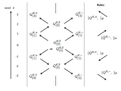
Figure 1: The tower of conserved charges. The absolute value of the level in the vertical axis measures the non-locality of the charges. The horizontal axis denotes eigenvalues of $Q^{R,3}_{(0)}$ . Higher-level charges can be constructed basically by taking the Poisson bracket according to the rules depicted in the figure, up to lower-level conserved charges.

3.4 Yangian limit

Since both the non-local currents $j_{\mu}^{R,\pm}(x)$ and $\tilde{j}_{\mu}^{R,\mp}(x)$ in (12) reduce to the local current $J^{\pm}_{\mu}(x)$ in $C\to 0$ limit, it is worth showing how the $SU(2)_{\rm R}$ Yangian charges obtained in KY are reproduced in this limit.

Interestingly, we have found that the rescaled differences of the corresponding charges recover the $(+,-)$-components of the $SU(2)_{\rm R}$ Yangian generators at level 1 recover as

$$\lim_{C\to 0}\frac{1}{2i\sqrt{C}}\left(Q^{R,+}_{(1)}-\widetilde{Q}^{R,+}_{(1)}\right)=\int\!\!dx\,J_{x}^{+}(x)-\frac{i}{2}\int\!\!\!\!\int\!\!dxdy\,\epsilon(x-y)\,J_{t}^{+}(x)J_{t}^{3}(y)\,,$$

$$\lim_{C\to 0}\frac{1}{2i\sqrt{C}}\left(\widetilde{Q}^{R,-}_{(1)}-Q^{R,-}_{(1)}\right)=\int\!\!dx\,J_{x}^{-}(x)+\frac{i}{2}\int\!\!\!\!\int\!\!dxdy\,\epsilon(x-y)\,J_{t}^{-}(x)J_{t}^{3}(y)\,.$$ (16)

The 3-component of the level 1 Yangian generators is reproduced as the $C\to 0$ limit of the difference of $Q_{(2)}^{R,3}$ and $\bar{Q}_{(2)}^{R,3}$

$$\lim_{C\to 0}\frac{i}{4}\left(Q^{R,3}_{(2)}-\bar{Q}_{(2)}^{R,3}\right) = \int\!\!dx\,J_{x}^{3}(x)+\frac{i}{2}\int\!\!\!\!\int\!\!dxdy\,\epsilon(x-y)\,J_{t}^{+}(x)J_{t}^{-}(y)\,.$$ (17)

Higher-level generators of the $SU(2)_{\rm R}$ Yangian are reproduced similarly.

In general, the level $n$ generators are obtained as the $C\to 0$ limit of the differences $Q^{R,+}_{(2n-1)}-\widetilde{Q}_{(2n-1)}^{R,+}$ , $\widetilde{Q}^{R,-}_{(2n-1)}-Q_{(2n-1)}^{R,-}$ and $Q^{R,3}_{(2n)}-\bar{Q}_{(2n)}^{R,3}$ for $n\geq 1$ . That is, half of the tower structure in Fig. 1 results in the $SU(2)_{\rm R}$ Yangian after taking the $C\to 0$ limit.

4 The classical origin of quantum affine algebra

In this section we will make some interpretations of the Poisson bracket algebra from the mathematical point of view. The first thing is that the Poisson brackets of the level $0,\pm 1$ charges in the previous section can be regarded as Drinfeld’s first realization of quantum affine algebra Drinfeld . Then we argue the role of the higher-level conserved charges in the context of the Drinfeld second realization Drinfeld .

4.1 Drinfeld’s first realization of quantum affine algebra

To see the relation to Drinfeld’s first realization Drinfeld , let us concentrate on the conserved charges $Q_{(0)}^{R,3}$ , $Q_{(1)}^{R,\pm}$ and $\widetilde{Q}_{(1)}^{R,\pm}$ , apart from the higher-level conserved charges $Q_{(n)}~{}(n\geq 2)$ . The role of the higher-level charges will be the subject in the next subsection.

It is convenient to rewrite the charges $Q_{(0)}^{R,3}$ , $Q_{(1)}^{R,\pm}$ and $\widetilde{Q}_{(1)}^{R,\pm}$ as follows:

$$\begin{array}[]{ll}H_{1}\equiv-2Q^{R,3}_{(0)}\,,&~{}~{}\qquad H_{0}\equiv 2Q^{R,3}_{(0)}\,,\\ E_{1}\equiv\left(\frac{\gamma}{\sinh(\gamma/2)}\right)^{1/2}Q^{R,+}_{(1)}\,,&~{}~{}\qquad E_{0}\equiv\left(\frac{\gamma}{\sinh(\gamma/2)}\right)^{1/2}\widetilde{Q}^{R,-}_{(1)}\,,\\ F_{1}\equiv\left(\frac{\gamma}{\sinh(\gamma/2)}\right)^{1/2}Q^{R,-}_{(1)}\,,&~{}~{}\qquad F_{0}\equiv\left(\frac{\gamma}{\sinh(\gamma/2)}\right)^{1/2}\widetilde{Q}^{R,+}_{(1)}\,.\end{array}$$

The Poisson brackets of them are

$$i\left\{H_{i},H_{j}\right\}_{\rm P}=0\qquad(i,j=0,1)\,,$$

$$i\left\{H_{i},E_{j}\right\}_{\rm P}=A_{ij}E_{j}\,,\qquad i\left\{H_{i},F_{j}\right\}_{\rm P}=-A_{ij}F_{j}\,,$$ (18)

$$i\left\{E_{i},F_{j}\right\}_{\rm P}=\delta_{ij}\frac{q^{H_{i}}-q^{-H_{i}}}{q-q^{-1}}\,.$$

Here the generalized Cartan matrix $A_{ij}$ is given by

$$A_{ij}=(\alpha_{i},\alpha_{j})=\begin{pmatrix}2&-2\\ -2&2\end{pmatrix}\quad\mbox{with}\quad\alpha_{1}=\begin{pmatrix}1\\ -1\end{pmatrix}\,,~{}~{}\alpha_{0}=\begin{pmatrix}-1\\ 1\end{pmatrix}$$ (19)

and a $q$-deformation parameter is defined as

$$q\equiv{\rm e}^{\gamma/2}=\exp\left(\frac{\sqrt{C}}{2(1+C)}\right)\,.$$ (20)

The brackets in (18) give a classical realization of the defining relations of quantum affine algebra in the sense of the first realization by Drinfeld Drinfeld . Its affine central charge $k$ is zero because

$$k\equiv H_{0}+H_{1}=0\,.$$

This corresponds to the evaluation representation of quantum affine algebra (see also CP ). Note that the $C\to 0$ limit is equivalent to $q\to 1$ .

The $q$-Serre relations should also be checked. The classical analogue of the $q$-Serre relations are deduced by introducing the classical $q$-Poisson bracket,

$$\left\{J^{A},J^{B}\right\}_{q{\rm P}}\equiv\left\{J^{A},J^{B}\right\}_{\rm P}+\frac{i\gamma}{2}\left(\beta_{A},\beta_{B}\right)J^{B}J^{A}\,,$$ (21)

where $\beta_{A}$ are the associated root vectors. Now $J^{A}$ and $J^{B}$ are $c$-number and commutative and the ordering in the second term is irrelevant. This $q$-Poisson bracket in (21) is nothing but a classical analogue of $q$-commutator and it is realized as a semiclassical limit ($\hbar\to 0$) of the $q$-commutator at quantum level, as we will see later.

With the $q$-Poisson bracket in (21), the classical $q$-Serre relations are shown as

$$\bigl{\{}E_{i},\bigl{\{}E_{i},\bigl{\{}E_{i},E_{j}\bigr{\}}_{q{\rm P}}\bigr{\}}_{q{\rm P}}\bigr{\}}_{q{\rm P}}=\bigl{\{}F_{i},\bigl{\{}F_{i},\bigl{\{}F_{i},F_{j}\bigr{\}}_{q{\rm P}}\bigr{\}}_{q{\rm P}}\bigr{\}}_{q{\rm P}}=0\quad{\rm for}~{}~{}|i-j|=1\,.$$

For the detail computation, see Appendix A.

4.2 The relation to the second realization

Next we shall make an interpretation of the higher-level conserved charges in the context of the Drinfeld second realization of quantum affine algebra Drinfeld .

Let us first introduce the following notation,

$$h_{0}\equiv-2Q^{R,3}_{(0)}\,,\qquad\quad x_{0}^{+}\equiv\sqrt{2}\,Q^{R,+}_{(1)}\,,\qquad\quad x_{0}^{-}\equiv\sqrt{2}\,Q^{R,-}_{(1)}\,,$$

$$x_{-1}^{+}\equiv\sqrt{2}\,{\rm e}^{\gamma Q^{R,3}_{(0)}}\,\widetilde{Q}^{R,+}_{(1)}\,,\qquad\quad x_{1}^{-}\equiv\sqrt{2}\,{\rm e}^{\gamma\bar{Q}^{R,3}_{(0)}}\,\widetilde{Q}^{R,-}_{(1)}\,.$$ (22)

Equivalently, the relations between $\left\{h_{k},x_{k}^{\pm}\right\}_{k\in{\mathbb{Z}}}$ and $H_{i},E_{i},F_{i}~{}(i=0,1)$ are written as

$$H_{1} =h_{0}\,, E_{1} =\left(\frac{\gamma/2}{\sinh(\gamma/2)}\right)^{1/2}x_{0}^{+}\,, F_{1} =\left(\frac{\gamma/2}{\sinh(\gamma/2)}\right)^{1/2}x_{0}^{-}\,,$$

$$H_{0} =-h_{0}\,, E_{0} =\left(\frac{\gamma/2}{\sinh(\gamma/2)}\right)^{1/2}{\rm e}^{-\gamma h_{0}/2}\,x_{1}^{-}\,, F_{0} =\left(\frac{\gamma/2}{\sinh(\gamma/2)}\right)^{1/2}{\rm e}^{\gamma h_{0}/2}\,x_{-1}^{+}\,.$$ (23)

This is the isomorphism from the first to the second realizations Drinfeld (see also CP ).

With the definitions in (22) and the Poisson brackets in (15), one can show that the following relations are satisfied,

$$\left\{h_{k},h_{l}\right\}_{\rm P}=0\,,\quad\left\{h_{k},x_{l}^{\pm}\right\}_{\rm P}=\mp 2ix_{k+l}^{\pm}\,,$$

$$\left\{x_{k+1}^{\pm},x_{l}^{\pm}\right\}_{\rm P}\pm i\gamma x_{l}^{\pm}x_{k+1}^{\pm}=\left\{x_{k}^{\pm},x_{l+1}^{\pm}\right\}_{\rm P}\mp i\gamma x_{k}^{\pm}x_{l+1}^{\pm}\,,$$

$$\left\{x_{k}^{+},x_{l}^{-}\right\}_{\rm P}=-\frac{i}{\gamma}\left(\psi_{k+l}^{+}-\psi_{k+l}^{-}\right)\,,$$

$$\sum_{k\in{\mathbb{Z}}}\psi_{k}^{\pm}z^{-k}={\rm e}^{\pm\gamma h_{0}/2}\exp\left(\pm\gamma\sum_{k=1}^{\infty}h_{\pm k}z^{\mp k}\right)\,.$$ (24)

This is nothing but a classical analogue of $U_{q}(\widehat{sl(2)})$ in the sense of the second realization. The root diagram of the conserved charges is depicted in Fig. 2.

The explicit expressions of higher charges can be computed from the above relations. For example, $h_{1}$ and $h_{-1}$ are obtained from $\left\{x_{0}^{+},x_{1}^{-}\right\}_{\rm P}$ and $\left\{x_{-1}^{+},x_{0}^{-}\right\}_{\rm P}$  respectively,

$$\bigl{\{}x_{0}^{+},x_{1}^{-}\bigr{\}}_{\rm P}=-\frac{i}{\gamma}\left(\psi_{1}^{+}-\psi_{1}^{-}\right)=-i{\rm e}^{h_{0}\gamma/2}h_{1}\,,$$

$$\bigl{\{}x_{-1}^{+},x_{0}^{-}\bigr{\}}_{\rm P}=-\frac{i}{\gamma}\left(\psi_{-1}^{+}-\psi_{-1}^{-}\right)=-i{\rm e}^{-h_{0}\gamma/2}h_{-1}\,,$$

and hence they can be written in terms of $Q_{(1)}^{R,\pm}$ and $\widetilde{Q}_{(1)}^{R,\pm}$ ,

$$h_{1} = 2i{\rm e}^{\gamma Q^{R,3}_{(0)}}\left\{Q^{R,+}_{(1)},{\rm e}^{\gamma\bar{Q}^{R,3}_{(0)}}\widetilde{Q}^{R,-}_{(1)}\right\}$$

$$= 2i\left\{Q^{R,+}_{(1)},\widetilde{Q}^{R,-}_{(1)}\right\}_{\rm P}-2\gamma Q^{R,+}_{(1)}\widetilde{Q}^{R,-}_{(1)}=-2i\left\{\widetilde{Q}^{R,-}_{(1)},Q^{R,+}_{(1)}\right\}_{q\rm P}\,,$$

$$h_{-1} = 2i{\rm e}^{\gamma\bar{Q}^{R,3}_{(0)}}\left\{{\rm e}^{\gamma Q^{R,3}_{(0)}}\widetilde{Q}^{R,+}_{(1)},Q^{R,-}_{(1)}\right\}$$

$$= 2i\left\{\widetilde{Q}^{R,+}_{(1)},Q^{R,-}_{(1)}\right\}_{\rm P}+2\gamma\widetilde{Q}^{R,+}_{(1)}Q^{R,-}_{(1)}=2i\left\{\widetilde{Q}^{R,+}_{(1)},Q^{R,-}_{(1)}\right\}_{q\rm P}\,.$$

Then $x_{k}^{\pm}~{}(k=1,2,3,\ldots)$ are constructed as a sequence obtained by acting $h_{\pm 1}$ on $x_{0}^{\pm}$ repeatedly,

$$\bigl{\{}h_{1},x_{k}^{\pm}\bigr{\}}_{\rm P}=\mp 2ix_{k+1}^{\pm}$$

$$\Longrightarrow \qquad x_{k}^{\pm}=\left(\pm\frac{i}{2}\right)^{k}\bigl{\{}h_{1},\bigl{\{}h_{1},\bigl{\{}\cdots,\bigl{\{}h_{1},x_{0}^{\pm}\bigr{\}}_{\rm P}\bigr{\}}_{\rm P}\bigr{\}}_{\rm P}\bigr{\}}_{\rm P}\,,$$

$$\bigl{\{}h_{-1},x_{-k}^{\pm}\bigr{\}}_{\rm P}=\mp 2ix_{-k-1}^{\pm}$$

$$\Longrightarrow \qquad x_{-k}^{\pm}=\left(\pm\frac{i}{2}\right)^{k}\bigl{\{}h_{-1},\bigl{\{}h_{-1},\bigl{\{}\cdots,\bigl{\{}h_{-1},x_{0}^{\pm}\bigr{\}}_{\rm P}\bigr{\}}_{\rm P}\bigr{\}}_{\rm P}\bigr{\}}_{\rm P}\,.$$

Since $x_{0}^{\pm}$ , $h_{1}$ and $h_{-1}$ are written in terms of $Q^{R,3}_{(0)}$ , $Q^{R,\pm}_{(1)}$ and $\widetilde{Q}^{R,\pm}_{(1)}$ , $x_{k}^{\pm}$ are also written in the same way. The Poisson brackets $\left\{A,B\right\}_{\rm P}$ above may be replaced by $q$-Poisson brackets $\left\{A,B\right\}_{q\rm P}$ , because the inner product of the root vectors associated with $\bigl{\{}Q^{R,\pm}_{(1)},\widetilde{Q}^{R,\mp}_{(1)}\bigr{\}}_{q\rm P}$ vanishes and there is no correction term in (21). In the end, all of $h_{k}$ are obtained from $x_{k}^{\pm}$ with the relations

$$\left\{x_{k-1}^{+},x_{1}^{-}\right\}_{\rm P}=\frac{\psi_{k}^{+}-\psi_{k}^{-}}{i\gamma}=-i{\rm e}^{\gamma h_{0}/2}h_{k}+\cdots\,,$$

$$\left\{x_{-1}^{+},x_{-k+1}^{-}\right\}_{\rm P}=\frac{\psi_{-k}^{+}-\psi_{-k}^{-}}{i\gamma}=-i{\rm e}^{\gamma h_{0}/2}h_{-k}+\cdots\,.$$

Here the part “$\dots$” contains only products of the lower-level conserved charges. The above argument proves the surjectivity of the map (23).

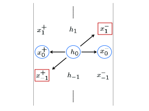
Figure 2: The tower structure of the conserved charges in the Drinfeld second realization. The three circles denote the $sl(2)$ root diagram and the two boxes are the associated affine generators. With the affine generators, higher conserved charges are basically generated according to the composition laws of vectors. First of all, $h_{1}$ is constructed as $h_{1}\sim\{x_{0}^{+},x_{1}^{-}\}_{\rm P}$ . Then $x_{1}^{+}$ is generated by $h_{1}$ and $x_{0}^{+}$ like $x_{1}^{+}\sim\{x_{0}^{+},h_{1}\}$ . The next step is to generate $h_{2}$ with $x_{1}^{+}$ and $x_{1}^{-}$ . After that $x_{2}^{\pm}$ are obtained by acting $x_{0}^{\pm}$ to $h_{2}$ , respectively. This step can be repeated recursively and the upper half of the tower is generated. The lower half is also generated in the same way.

Let us here comment on the relation between the second realization of quantum affine algebra and the higher-level conserved charges obtained by expanding the monodromy matrix $U^{R}(\lambda)$ in (7). By construction, $x^{\pm}_{\pm k}$ and $h_{\pm k}$ are written as a sequence of the Poisson brackets among $Q^{R,\pm}_{(1)}$ and $\widetilde{Q}^{R,\pm}_{(1)}$ . Hence it is easy to notice that $x^{\pm}_{\pm k}$ and $h_{\pm k}$ are closely related to the higher-level conserved charges obtained by expanding the monodromy matrix. For example, $h_{1}$ and $h_{-1}$ correspond to $Q_{(2)}^{R,3}$ and $\bar{Q}_{(2)}^{R,3}$ , respectively, up to the lower-level conserved charges. Similarly, one can figure out the correspondence between the charges in Fig. 1 and in Fig. 2, up to lower-level conserved charges.

Note that there is an ambiguity in the expression of the monodromy matrix in (7) according to an ambiguity of the Lax pair due to gauge transformations. It may be possible to figure out the exact correspondence without deviation by lower-level conserved charges. However, it has not been done yet so far. As a peculiarity of $U_{q}(\widehat{sl(2)})$ , the width of the root diagram shown in Fig. 2 is not so wide that such an exact correspondence may be found out. It would be an interesting direction in the future study. It is also nice to elucidate the relation to the RTT formalism, following DF .

5 Comment on semiclassical limit

Although we have focused upon classical realizations of quantum affine algebra so far, the next subject is to consider a semiclassical limit of quantum affine algebra realized at quantum mechanical level. In principle, one can perform the canonical quantization by replacing the classical Poisson bracket with the usual commutator like

$$i\{~{}~{},~{}~{}\}_{\rm P}~{}~{}\rightarrow~{}~{}\frac{1}{\hbar}[~{}~{},~{}~{}]\,.$$

Then a quantum affine algebra seems to be realized at quantum level but it is not the case. The conservation laws of non-local charges should be checked carefully, because their definition contains the product of currents and hence some renormalizations are necessary to define the charges at quantum level definitely. Namely, the conservation laws might be broken due to the renormalization after all. In the case of $O(N)$ non-linear sigma models in two dimensions, the quantum conservation laws are carefully confirmed Luscher1 (For generic coset sigma models, see GW ; AFG ).

Eventually, the quantum conservation laws should be shown for definite argument by following GW ; AFG in the present case. Then it is possible to discuss the quantum affine algebra along the scenario as discussed in Bernard . We do not, however, try to argue the conservation laws in detail here and leave it as a future problem. Instead, simply supposing that well-defined quantum charges $\widehat{Q}$’s exist, we discuss a semiclassical limit of quantum affine algebra realized at quantum level.

Note that, for quantum integrability of squashed sigma model, we have another confirmation, which is that the Bethe ansatz has already been constructed by Wiegmann quantum1 (For related works see quantum2 ; quantum3 ) and the exact solutions have been found out. As a result, the quantum integrability has been confirmed indirectly by another argument.

For simplicity, we consider the first realization of quantum affine algebra here. Then the quantum charges satisfy the defining relations of $U_{q}(\widehat{sl(2)})$ , which are the standard form in mathematical literatures, like

$$\bigl{[}\widehat{H}_{i},\widehat{H}_{j}\bigr{]}=0\qquad(i,j=0,1)\,,$$

$$\bigl{[}\widehat{H}_{i},\widehat{E}_{j}\bigr{]}=A_{ij}\widehat{E}_{j}\,,\qquad\bigl{[}\widehat{H}_{i},\widehat{F}_{j}\bigr{]}=-A_{ij}\widehat{F}_{j}\,,$$ (25)

$$\bigl{[}\widehat{E}_{i},\widehat{F}_{j}\bigr{]}=\delta_{ij}\frac{\widehat{q}^{H_{i}}-\widehat{q}^{-H_{i}}}{\widehat{q}-\widehat{q}^{-1}}\,.$$

The $q$-Serre relations are

$$\bigl{[}\widehat{E}_{i},\bigl{[}\widehat{E}_{i},\bigl{[}\widehat{E}_{i},\widehat{E}_{j}\bigr{]}_{\widehat{q}}\bigr{]}_{\widehat{q}}\bigr{]}_{\widehat{q}}=\bigl{[}\widehat{F}_{i},\bigl{[}\widehat{F}_{i},\bigl{[}\widehat{F}_{i},\widehat{F}_{j}\bigr{]}_{\widehat{q}}\bigr{]}_{\widehat{q}}\bigr{]}_{\widehat{q}}=0\qquad{\rm for}\quad|i-j|=1\$$ (26)

and the $q$-commutator is defined as

$$[\widehat{J}^{A},\widehat{J}^{B}]_{\widehat{q}}\equiv\widehat{J}^{A}\widehat{J}^{B}-\widehat{q}^{(\beta_{A},\beta_{B})}\widehat{J}^{B}\widehat{J}^{A}\,.$$ (27)

Here a deformation parameter $\widehat{q}$ at quantum level is related to the classical one $q$ as

$$\widehat{q}\equiv q^{\hbar}={\rm e}^{\hbar\gamma/2}\,.$$ (28)

Note that $\widehat{q}$ depends on the Planck constant $\hbar$ . This is a difference of importance between at classical and quantum levels.

Let us now consider a semiclassical limit $\hbar\to 0$ . The quantum charges are first rescaled as

$$\widehat{E}_{i}\rightarrow\hbar\left(\frac{\gamma}{\sinh(\gamma/2)}\right)^{1/2}\widehat{E}_{i}\,,\quad\widehat{F}_{i}\rightarrow\hbar\left(\frac{\gamma}{\sinh(\gamma/2)}\right)^{1/2}\widehat{F}_{i}\,,\quad\widehat{H}_{i}\rightarrow\frac{\hbar}{2}\widehat{H}_{i}\,,$$

and then the commutators should be replaced by the Poisson brackets,

$$\left[\quad,\quad\right]~{}~{}\rightarrow~{}~{}i\hbar\left\{\quad,\quad\right\}_{\rm P}\,.$$

Noting that $\widehat{q}$ is expanded with respect to $\hbar$ as

$$\widehat{q}=1+\frac{\hbar\gamma}{2}+\mathcal{O}(\hbar^{2})\,,$$

the semiclassical limit $\hbar\to 0$ is taken.

As a result, the classical defining relations in (18) are reproduced as a semiclassical limit of the quantum ones in (25) , as a matter of course. In addition, the classical $q$-Poisson bracket in (21) is reproduced as a semiclassical limit of the standard $q$-commutator (27):

$$[\widehat{J}^{A},\widehat{J}^{B}]_{\widehat{q}} = \widehat{J}^{A}\widehat{J}^{B}-\widehat{q}^{(\beta_{A},\beta_{B})}\widehat{J}^{B}\widehat{J}^{A}$$

$$= [\widehat{J}^{A},\widehat{J}^{B}]-({\rm e}^{\hbar\gamma(\beta_{A},\beta_{B})/2}-1)\widehat{J}^{B}\widehat{J}^{A}$$

$$\rightarrow i\hbar\{J^{A},J^{B}\}_{\rm P}-\frac{\hbar\gamma}{2}(\beta_{A},\beta_{B})J^{B}J^{A}$$

$$= i\hbar\{J^{A},J^{B}\}_{q{\rm P}}$$

6 Conclusion and Discussion

We have argued a quantum affine algebra realized in two-dimensional non-linear sigma models with target space three-dimensional squashed spheres. We have explicitly constructed its affine generators and computed the Poisson brackets. The defining relations of quantum affine algebra in the sense of the Drinfeld first realization are satisfied at classical level. The relation to the second realization is also discussed including higher conserved charges. The result here is consistently interpreted as a semiclassical limit of quantum affine algebra realized at quantum level.

There are some potentially interesting directions in the future study. The first is to figure out an affine extension of $q$-deformed Poincare symmetry in the null-warped case KY-Sch by following the argument discussed here. It is also nice to consider an extension of the null-warped geometry to the higher-dimensional case, though the coset structure is not reductive any more in contrast to the three-dimensional case SYY . A relative direction is to consider the hybrid deformation consisting of the standard $q$-deformed $SL(2)$ and the $q$-deformed Poincare BHP (For its application to three-dimensional gravities see BHM ).

The second is to look for some applications in the context of AdS/condensed matter physics (CMP), where the warped AdS geometries appear as the gravity dual to the system in the presence of magnetic field Kraus . The anisotropy of the system is reflected as the squashing of spacetime geometry in the gravity side. Finally, it is interesting to try to consider quantum affine algebra in the context of Kerr/CFT correspondence Kerr/CFT and the recently proposed scenario, warped AdS₃/dipole CFT₂ Guica ; SS .

It is also a nice direction to consider the string-theory embedding by following the works Detournay1 ; Detournay2 and consider the role of quantum affine algebra presented here in the string-theory context. In this direction, first of all, we should be careful for the conformal invariance. The squashed sigma model is not conformal and hence we have to add the Wess-Zumino (WZ) term. We have already shown that the $SU(2)_{\rm L}$ Yangian algebra is still preserved even after adding the WZ term KOY . However, the quantum affine algebra in the presence of the WZ term has not been investigated yet. It is the next issue and we hope that we could report on it in the near future.

Acknowledgments

We would like to thank H. Kawai, S. Moriyama and T. Okada for illuminating discussions. This work was initiated in the workshop, under the program “Synthesis of integrabilities arising from gauge-string duality,” held at Higher School of Economics and Steklov Mathematical Institute in Moscow, Russia. We greatly appreciate the organizers’ hospitality, including H. Itoyama and A. Morozov. The work of IK was supported by the Japan Society for the Promotion of Science (JSPS). The work of KY was supported by the scientific grants from the Ministry of Education, Culture, Sports, Science and Technology (MEXT) of Japan (No. 22740160). This work was also supported in part by the Grant-in-Aid for the Global COE Program “The Next Generation of Physics, Spun from Universality and Emergence” from MEXT, Japan. One of the authors TM is also grateful to A. Molev for valuable comments on this work. Part of his work was done during “2nd Asia-Pacific Summer School in Mathematical Physics, 22nd Canberra International Physics Summer School CFT, AdS/CFT and Integrability” held at the Australian National University in Canberra, Australia. He would like to thank the organizers and the lecturers C. Ahn, V. Bazhanov and R. Nepomechie for kindly answering his basic questions related to the subject of this paper.

Appendix

Appendix A Proof of $q$-Serre relations at classical level

We show here that $E_{i}$ and $F_{i}$ satisfy the classical analogue of $q$-Serre relations in (4.1). Note that the $q$-Serre relations are rewritten with $Q^{R,\pm}_{(1)}$ and $\widetilde{Q}^{R,\pm}_{(1)}$ as

$$\bigl{\{}Q^{R,\pm}_{(1)},\bigl{\{}Q^{R,\pm}_{(1)},\bigl{\{}Q^{R,\pm}_{(1)},\widetilde{Q}^{R,\mp}_{(1)}\bigr{\}}_{q{\rm P}}\bigr{\}}_{q{\rm P}}\bigr{\}}_{q{\rm P}}=0\,,$$ (29)

$$\bigl{\{}\widetilde{Q}^{R,\mp}_{(1)},\bigl{\{}\widetilde{Q}^{R,\mp}_{(1)},\bigl{\{}\widetilde{Q}^{R,\mp}_{(1)},Q^{R,\pm}_{(1)}\bigr{\}}_{q{\rm P}}\bigr{\}}_{q{\rm P}}\bigr{\}}_{q{\rm P}}=0\,.$$ (30)

The first bracket is evaluated as

$$\bigl{\{}Q^{R,\pm}_{(1)},\widetilde{Q}^{R,\mp}_{(1)}\bigr{\}}_{q{\rm P}} = \bigl{\{}Q^{R,\pm}_{(1)},\widetilde{Q}^{R,\mp}_{(1)}\bigr{\}}_{\rm P}+\frac{i\gamma}{2}\left(\alpha_{0},\alpha_{1}\right)\widetilde{Q}^{R,\mp}_{(1)}Q^{R,\pm}_{(1)}$$

$$= \bigl{\{}Q^{R,\pm}_{(1)},\widetilde{Q}^{R,\mp}_{(1)}\bigr{\}}_{\rm P}-i\gamma\widetilde{Q}^{R,\mp}_{(1)}Q^{R,\pm}_{(1)}\,.$$

Then one more bracket leads to

$$\bigl{\{}Q^{R,\pm}_{(1)},\bigl{\{}Q^{R,\pm}_{(1)},\widetilde{Q}^{R,\mp}_{(1)}\bigr{\}}_{q{\rm P}}\bigr{\}}_{q{\rm P}}$$

$$= \bigl{\{}Q^{R,\pm}_{(1)},\bigl{\{}Q^{R,\pm}_{(1)},\widetilde{Q}^{R,\mp}_{(1)}\bigr{\}}_{q{\rm P}}\bigr{\}}_{\rm P}+\frac{i\gamma}{2}\left(\alpha_{0},\alpha_{0}+\alpha_{1}\right)\bigl{\{}Q^{R,\pm}_{(1)},\widetilde{Q}^{R,\mp}_{(1)}\bigr{\}}_{q{\rm P}}Q^{R,\pm}_{(1)}$$

$$= \bigl{\{}Q^{R,\pm}_{(1)},\bigl{\{}Q^{R,\pm}_{(1)},\widetilde{Q}^{R,\mp}_{(1)}\bigr{\}}_{q{\rm P}}\bigr{\}}_{\rm P}\,.$$

With one more bracket, we obtain that

$$\bigl{\{}Q^{R,\pm}_{(1)},\bigl{\{}Q^{R,\pm}_{(1)},\bigl{\{}Q^{R,\pm}_{(1)},\widetilde{Q}^{R,\mp}_{(1)}\bigr{\}}_{q{\rm P}}\bigr{\}}_{q{\rm P}}\bigr{\}}_{q{\rm P}}$$

$$= \bigl{\{}Q^{R,\pm}_{(1)},\bigl{\{}Q^{R,\pm}_{(1)},\bigl{\{}Q^{R,\pm}_{(1)},\widetilde{Q}^{R,\mp}_{(1)}\bigr{\}}_{q{\rm P}}\bigr{\}}_{q{\rm P}}\bigr{\}}_{\rm P}$$

$$\quad+\frac{i\gamma}{2}\left(\alpha_{0},2\alpha_{0}+\alpha_{1}\right)\bigl{\{}Q^{R,\pm}_{(1)},\bigl{\{}Q^{R,\pm}_{(1)},\widetilde{Q}^{R,\mp}_{(1)}\bigr{\}}_{q{\rm P}}\bigr{\}}_{q{\rm P}}Q^{R,\pm}_{(1)}$$

$$= \bigl{\{}Q^{R,\pm}_{(1)},\bigl{\{}Q^{R,\pm}_{(1)},\bigl{\{}Q^{R,\pm}_{(1)},\widetilde{Q}^{R,\mp}_{(1)}\bigr{\}}_{q{\rm P}}\bigr{\}}_{q{\rm P}}\bigr{\}}_{\rm P}+i\gamma\bigl{\{}Q^{R,\pm}_{(1)},\bigl{\{}Q^{R,\pm}_{(1)},\widetilde{Q}^{R,\mp}_{(1)}\bigr{\}}_{q{\rm P}}\bigr{\}}_{q{\rm P}}Q^{R,\pm}_{(1)}\,.$$

The fourth bracket is evaluated as

$$\bigl{\{}Q^{R,\pm}_{(1)},\bigl{\{}Q^{R,\pm}_{(1)},\bigl{\{}Q^{R,\pm}_{(1)},\widetilde{Q}^{R,\mp}_{(1)}\bigr{\}}_{q{\rm P}}\bigr{\}}_{q{\rm P}}\bigr{\}}_{q{\rm P}}$$

$$= \bigl{\{}Q^{R,\pm}_{(1)},\bigl{\{}Q^{R,\pm}_{(1)},\bigl{\{}Q^{R,\pm}_{(1)},\widetilde{Q}^{R,\mp}_{(1)}\bigr{\}}_{q{\rm P}}\bigr{\}}_{q{\rm P}}\bigr{\}}_{\rm P}+i\gamma\bigl{\{}Q^{R,\pm}_{(1)},\bigl{\{}Q^{R,\pm}_{(1)},\widetilde{Q}^{R,\mp}_{(1)}\bigr{\}}_{q{\rm P}}\bigr{\}}_{q{\rm P}}Q^{R,\pm}_{(1)}$$

$$= \bigl{\{}Q^{R,\pm}_{(1)},\bigl{\{}Q^{R,\pm}_{(1)},\bigl{\{}Q^{R,\pm}_{(1)},\widetilde{Q}^{R,\mp}_{(1)}\bigr{\}}_{q{\rm P}}\bigr{\}}_{\rm P}\bigr{\}}_{\rm P}+i\gamma\bigl{\{}Q^{R,\pm}_{(1)},\bigl{\{}Q^{R,\pm}_{(1)},\widetilde{Q}^{R,\mp}_{(1)}\bigr{\}}_{q{\rm P}}\bigr{\}}_{\rm P}Q^{R,\pm}_{(1)}$$

$$= \bigl{\{}Q^{R,\pm}_{(1)},\bigl{\{}Q^{R,\pm}_{(1)},\bigl{\{}Q^{R,\pm}_{(1)},\widetilde{Q}^{R,\mp}_{(1)}\bigr{\}}_{\rm P}-i\gamma\widetilde{Q}^{R,\mp}_{(1)}Q^{R,\pm}_{(1)}\bigr{\}}_{\rm P}\bigr{\}}_{\rm P}$$

$$\quad+i\gamma\bigl{\{}Q^{R,\pm}_{(1)},\bigl{\{}Q^{R,\pm}_{(1)},\widetilde{Q}^{R,\mp}_{(1)}\bigr{\}}_{\rm P}-i\gamma\widetilde{Q}^{R,\mp}_{(1)}Q^{R,\pm}_{(1)}\bigr{\}}_{\rm P}Q^{R,\pm}_{(1)}$$

$$= \bigl{\{}Q^{R,\pm}_{(1)},\bigl{\{}Q^{R,\pm}_{(1)},\bigl{\{}Q^{R,\pm}_{(1)},\widetilde{Q}^{R,\mp}_{(1)}\bigr{\}}_{\rm P}\bigr{\}}_{\rm P}\bigr{\}}_{\rm P}+\gamma^{2}\bigl{\{}Q^{R,\pm}_{(1)},\widetilde{Q}^{R,\mp}_{(1)}\bigr{\}}_{\rm P}(Q^{R,\pm}_{(1)})^{2}\,.$$

With the Poisson brackets in (15), one can show the following:

$$\bigl{\{}Q^{R,\pm}_{(1)},\bigl{\{}Q^{R,\pm}_{(1)},\bigl{\{}Q^{R,\pm}_{(1)},\widetilde{Q}^{R,\mp}_{(1)}\bigr{\}}_{\rm P}\bigr{\}}_{\rm P}\bigr{\}}_{\rm P}+\gamma^{2}\bigl{\{}Q^{R,\pm}_{(1)},\widetilde{Q}^{R,\mp}_{(1)}\bigr{\}}_{\rm P}(Q^{R,\pm}_{(1)})^{2}=0\,.$$

Thus the relation (29) has been proven. Similarly, one can easily show the relation (30).

References

• (1) M. L$\ddot{\rm u}$scher, “Quantum nonlocal charges and absence of particle production in the two-dimensional nonlinear sigma model,” Nucl. Phys.  B 135 (1978) 1.
• (2) M. L$\ddot{\rm u}$scher and K. Pohlmeyer, “Scattering of massless lumps and nonlocal charges in the two-dimensional classical nonlinear sigma model,” Nucl. Phys.  B 137 (1978) 46.
• (3) E. Abdalla, M. C. Abdalla and K. Rothe, “Non-perturbative methods in two-dimensional quantum field theory,” World Scientific, 1991.
• (4) E. Brezin, C. Itzykson, J. Zinn-Justin and J. B. Zuber, “Remarks about the existence of nonlocal charges in two-dimensional models,” Phys. Lett.  B 82 (1979) 442.
• (5) D. Bernard, “Hidden Yangians in 2-D massive current algebras,” Commun. Math. Phys. 137 (1991) 191.
• (6) N. J. MacKay, “On the classical origins of Yangian symmetry in integrable field theory,” Phys. Lett. B 281 (1992) 90 [Erratum-ibid. B 308 (1993) 444].
• (7) V. G. Drinfel’d, “Hopf algebras and the quantum Yang-Baxter equation,” Sov. Math. Dokl. 32 (1985) 254; “Quantum groups,” J. Sov. Math.  41 (1988) 898 [Zap. Nauchn. Semin.  155, 18 (1986)]; “A new realization of Yangians and quantized affine algebras,” Sov. Math. Dokl.  36 (1988) 212.
• (8) Y. Y. Goldschmidt and E. Witten, “Conservation laws in some two-dimensional models,” Phys. Lett.  B 91 (1980) 392.
• (9) E. Abdalla, M. Forger and M. Gomes, “On the origin of anomalies in the quantum nonlocal charge for the generalized nonlinear sigma models,” Nucl. Phys.  B 210 (1982) 181.
• (10) A. Polyakov and P. B. Wiegmann, “Theory of non-abelian Goldstone bosons in two dimensions,” Phys. Lett. B 131 (1983) 121.
• (11) J. M. Maldacena, “The large N limit of superconformal field theories and supergravity,” Adv. Theor. Math. Phys.  2 (1998) 231 [Int. J. Theor. Phys.  38 (1999) 1113]. [arXiv:hep-th/9711200].
• (12) N. Beisert et al., “Review of AdS/CFT Integrability: An Overview,” arXiv:1012.3982 [hep-th].
• (13) I. Bena, J. Polchinski and R. Roiban, “Hidden symmetries of the AdS${}_{5}\times S^{5}$ superstring,” Phys. Rev.  D 69 (2004) 046002. [arXiv:hep-th/0305116].
• (14) K. Zarembo, “Strings on semisymmetric superspaces,” JHEP 1005 (2010) 002. [arXiv:1003.0465 [hep-th]].
• (15) R. G. Leigh and M. J. Strassler, “Exactly marginal operators and duality in four-dimensional N=1 supersymmetric gauge theory,” Nucl. Phys.  B 447 (1995) 95 [arXiv:hep-th/9503121].
• (16) O. Lunin and J. M. Maldacena, “Deforming field theories with $U(1)\times U(1)$ global symmetry and their gravity duals,” JHEP 0505 (2005) 033 [arXiv:hep-th/0502086].
• (17) S. Frolov, “Lax pair for strings in Lunin-Maldacena background,” JHEP 0505 (2005) 069 [arXiv:hep-th/0503201].
• (18) D. Berenstein and D. H. Correa, “Emergent geometry from $q$-deformations of N=4 super Yang-Mills,” JHEP 0608 (2006) 006 [arXiv:hep-th/0511104].
• (19) N. Beisert and P. Koroteev, “Quantum Deformations of the One-Dimensional Hubbard Model,” J. Phys. A A 41 (2008) 255204 [arXiv:0802.0777 [hep-th]].
• (20) N. Beisert, W. Galleas and T. Matsumoto, “A Quantum Affine Algebra for the Deformed Hubbard Chain,” arXiv:1102.5700 [math-ph].
• (21) B. Hoare, T. J. Hollowood and J. L. Miramontes, “q-Deformation of the $AdS_{5}xS^{5}$ Superstring S-matrix and its Relativistic Limit,” arXiv:1112.4485 [hep-th].
• (22) I. Kawaguchi and K. Yoshida, “Hidden Yangian symmetry in sigma model on squashed sphere,” JHEP 1011 (2010) 032. [arXiv:1008.0776 [hep-th]].
• (23) I. Kawaguchi, D. Orlando and K. Yoshida, “Yangian symmetry in deformed WZNW models on squashed spheres,” Phys. Lett.  B 701 (2011) 475. [arXiv:1104.0738 [hep-th]].
• (24) I. Kawaguchi and K. Yoshida, “Hybrid classical integrability in squashed sigma models,” Phys. Lett. B 705 (2011) 251 [arXiv:1107.3662 [hep-th]].
• (25) I. Kawaguchi and K. Yoshida, “Hybrid classical integrable structure of squashed sigma models: A Short summary,” arXiv:1110.6748 [hep-th].
• (26) M. Jimbo, “A $q$ difference analog of $U(g)$ and the Yang-Baxter equation,” Lett. Math. Phys.  10 (1985) 63.
• (27) L. D. Faddeev and N. Y. Reshetikhin, “Integrability of the principal chiral field model in (1+1)-dimension,” Annals Phys.  167 (1986) 227.
• (28) D. Orlando, S. Reffert and L. I. Uruchurtu, “Classical integrability of the squashed three-sphere, warped AdS3 and Schr$\ddot{\rm o}$dinger spacetime via T-Duality,” J. Phys. A 44 (2011) 115401. [arXiv:1011.1771 [hep-th]].
• (29) V. Chari and A. Pressley, “Quantum affine algebras,” Commun. Math. Phys. 142 (1991) 261.
• (30) J. Ding and I. B. Frenkel, “Isomorphism of two realizations of quantum affine algebra $U_{q}(\widehat{gl(n)})$ ” Commun. Math. Phys. 156 (1993) 277.
• (31) D. Bernard and A. Leclair, “Quantum group symmetries and nonlocal currents in 2-D QFT,” Commun. Math. Phys.  142 (1991) 99.
• (32) P. B. Wiegmann, “Exact solution of the O(3) nonlinear sigma model,” Phys. Lett.  B 152 (1985) 209.
• (33) V. A. Fateev, “The sigma model (dual) representation for a two-parameter family of integrable quantum field theories,” Nucl. Phys.  B 473 (1996) 509.
• (34) J. Balog and P. Forgacs, “Thermodynamical Bethe ansatz analysis in an $SU(2)\times U(1)$ symmetric sigma model,” Nucl. Phys.  B 570 (2000) 655 [arXiv:hep-th/9906007].
• (35) I. Kawaguchi and K. Yoshida, “Classical integrability of Schrodinger sigma models and q-deformed Poincare symmetry,” JHEP 1111 (2011) 094 [arXiv:1109.0872 [hep-th]].
• (36) S. Schafer-Nameki, M. Yamazaki and K. Yoshida, “Coset construction for duals of non-relativistic CFTs,” JHEP 0905 (2009) 038. [arXiv:0903.4245 [hep-th]].
• (37) A. Ballesteros, F. J. Herranz and P. Parashar, “Multiparametric quantum $gl(2)$: Lie bialgebras, quantum $R$-matrices and non-relativistic limits,” J. Phys. A 32 (1999) 2369.
• (38) A. Ballesteros, F. J. Herranz and C. Meusburger, “Three-dimensional gravity and Drinfel’d doubles: spacetimes and symmetries from quantum deformations,” Phys. Lett. B 687 (2010) 375 [arXiv:1001.4228 [gr-qc]].
• (39) E. D’Hoker and P. Kraus, “Charged magnetic brane solutions in AdS5 and the fate of the third law of thermodynamics,” JHEP 1003 (2010) 095;
[arXiv:0911.4518 [hep-th]]; “Holographic metamagnetism, quantum criticality, and crossover behavior,” JHEP 1005 (2010) 083. [arXiv:1003.1302 [hep-th]].
• (40) M. Guica, T. Hartman, W. Song and A. Strominger, “The Kerr/CFT correspondence,” Phys. Rev.  D 80 (2009) 124008. [arXiv:0809.4266 [hep-th]].
• (41) S. El-Showk and M. Guica, “Kerr/CFT, dipole theories and nonrelativistic CFTs,” arXiv:1108.6091 [hep-th].
• (42) W. Song and A. Strominger, “Warped AdS3/Dipole-CFT Duality,” arXiv:1109.0544 [hep-th].
• (43) S. Detournay, D. Israel, J. M. Lapan and M. Romo, “String Theory on Warped AdS3 and Virasoro Resonances,” JHEP 1101 (2011) 030 [arXiv:1007.2781 [hep-th]].
• (44) S. Detournay, J. M. Lapan and M. Romo, “SUSY Enhancements in (0,4) Deformations of AdS3/CFT2,” JHEP 1201 (2012) 006 [arXiv:1109.4186 [hep-th]].