Existence of negative differential thermal conductance in one-dimensional diffusive thermal transport

Abstract

We show that in a finite one-dimensional (1D) system with diffusive thermal transport described by the Fourier’s law, negative differential thermal conductance (NDTC) cannot occur when the temperature at one end is fixed. We demonstrate that NDTC in this case requires the presence of junction(s) with temperature dependent thermal contact resistance (TCR). We derive a necessary and sufficient condition for the existence of NDTC in terms of the properties of the TCR for systems with a single junction. We show that under certain circumstances we even could have infinite (negative or positive) differential thermal conductance in the presence of the TCR. Our predictions provide theoretical basis for constructing NDTC-based devices, such as thermal amplifiers, oscillators and logic devices.

In recent years, nonlinear thermal transport, particularly in low dimensional systems, is of significant interest from both fundamental and practical perspectives Lepri et al. (2003); Li et al. (2012). For example, thermal rectification has been experimentally and theoretically studied in many nanostructures Terraneo et al. (2002); Eckmann and Mejía-Monasterio (2006); Li et al. (2004); Casati et al. (2007); Peyrard (2006); Chang et al. (2006); Yang et al. (2007); Hu et al. (2009); Pereira (2010) and heterogeneous bulk materials Sawaki et al. (2011); Go and Sen (2010); Dames (2009). Negative differential thermal conductance (NDTC), an unusual thermal transport phenomenon where the heat current across a thermal conductor decreases when the temperature bias increases, is an essential element for the construction of thermal transistors Li et al. (2006) and thermal logic Wang and Li (2007), and is shown to exist in many non-linear one-dimensional (1D) systems Li et al. (2006); Yang et al. (2007); He et al. (2009); Zhong et al. (2009); Shao et al. (2009); He et al. (2010); Pereira (2010); Ai and Hu (2011); Ai et al. (2011); Hu et al. (2011); Shao and Yang (2011) and vacuum gaps Zhu et al. (2012). Many mechanisms such as nonlinear interactions Segal (2006), molecular anharmonicity Wu et al. (2009); Ai and Hu (2011); Ai et al. (2011); Pereira (2010), interplay between the thermal driving force and the thermal (boundary) conductance He et al. (2009, 2010); Zhong et al. (2009); Hu et al. (2011), thermal interfaces Li et al. (2006); Shao et al. (2009); He et al. (2009) and others Zhu et al. (2012) have been proposed to explain the existence of NDTC. Interestingly, several numerical studies Shao et al. (2009); Zhong et al. (2009); He et al. (2010); Hu et al. (2011) have suggested that NDTC may vanish as the system length becomes large (approaching diffusive thermal transport). However, it has not been definitely answered whether NDTC universally vanishes for diffusive thermal transport. Besides, the role played by thermal interfaces in NDTC has not been well studied. Here, we provide a generic and analytic study of these issues in 1D diffusive thermal transport described by the Fourier’s law. We prove that NDTC cannot exist when the temperature at one end is fixed. However, we show that NDTC in this case is still possible if a junction with temperature dependent thermal contact resistance (TCR) is introduced. Unlike previous theories and simulations Li et al. (2006); Yang et al. (2007); He et al. (2009); Zhong et al. (2009); Shao et al. (2009); He et al. (2010); Pereira (2010); Ai and Hu (2011); Ai et al. (2011); Hu et al. (2011); Shao and Yang (2011) that dealt with specific toy models which are often difficult to access experimentally, our predictions provide a generic way towards building NDTC-based devices.

We consider a general 1D system in the diffusive thermal transport regime whose thermal conductivity $\kappa(x,T)$ is a function of the coordinate $x$ and the local temperature $T(x)$. The position dependence of the thermal conductivity $\kappa(x,T)$ is explicitly expressed, since the system we consider can have a spatial dependence of structure or composition (e.g., strain or mass gradient). This phenomenological description is valid as long as the mean free path (MFP) of heat carriers is much smaller than the size of the system, where the microscopic details are unimportant. This approach generates analytic results regarding the existence of NDTC, and it is instructive in system design to pursue the applications of NDTC.

For a finite 1D system which lies in the coordinate range $[x^{L},x^{R}]$ (Fig. 1), the local heat current $q(x)$ can be calculated from the Fourier’s law:

$$q(x)=-\kappa(x,T)\frac{\mathrm{d}T}{\mathrm{d}x}.$$ (1)

For thermal transport without heat sources or sinks, the heat current is conserved and the steady state thermal transport equation reads

$$\frac{\mathrm{d}}{\mathrm{d}x}\left(\kappa(x,T)\frac{\mathrm{d}T}{\mathrm{d}x}\right)=0.$$ (2)

Once the temperature at two ends of the system are given, i.e.,

$$T\left(x^{L(R)}\right)=T^{L(R)},$$ (3)

the temperature profile $T(x)$ is uniquely Walter and Thompson (1998) determined by Eq. (2) and the boundary conditions (3), and the resulting heat current $q$ (independent of $x$) flowing in the system can be computed from Eq. (1).

By applying an infinitesimal variation $\delta T^{L(R)}$ of the boundary temperature at one end, i.e., $T^{L(R)}$ is varied to $T^{L(R)}+\delta T^{L(R)}$ while the temperature $T^{R(L)}$ at the other end is fixed, the resulting temperature profile is varied to $T(x)+\delta T(x)$. This temperature profile variation $\delta T(x)$ can induce a variation $\delta q$ of the heat current. We define the differential thermal conductance (DTC) as

$$G\equiv\frac{\delta q}{\delta(T^{L}-T^{R})},$$ (4)

or specifically

$$G=G^{L}=\frac{\delta q}{\delta T^{L}},\;\;\;\;\;\text{when}\;T^{R}\;\text{is fixed; or}$$ (5)

$$G=G^{R}=-\frac{\delta q}{\delta T^{R}},\;\;\text{when}\;T^{L}\;\text{is fixed}.$$

In the following we consider the cases with and without the junctions to discuss the existence of NDTC.

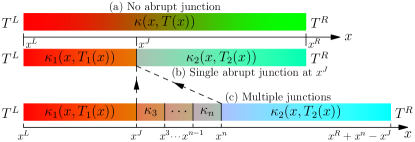
Figure 1: Schematics of 1D systems without any junctions (a) and with a single junction (b) and multiple junctions (c). The junctions are indicated by vertical black lines.

Systems without abrupt junctions, as shown in Fig. 1(a). In this case, if $T^{R(L)}$ is fixed (without loss of generality, we can assume $T^{L}>T^{R}$), we will show that there is no NDTC and the heat current $q$ will increase as the temperature bias increases by increasing (lowering) $T^{L(R)}$ (NDTC could still exist when the temperatures at two ends vary simultaneously not (a), however, we limit our study in the cases that the temperature at one end is fixed).

Qualitatively, we first point out that the non-existence of NDTC here is a direct consequence of the uniqueness of the solution of Eq. (2), as we graphically demonstrate in Fig. 2(a). Take the case that $T^{R}$ is fixed as an example. If the temperature $T^{L}$ is increased to $T^{\prime L}$ ($>T^{L}$), the temperature profile $T(x)$ (black line) with $T(x^{L(R)})=T^{L(R)}$ and heat current $q$ are changed to $T^{\prime}(x)$ (red line) with $T^{\prime}(x^{L})=T^{\prime L}$ and $T^{\prime}(x^{R})=T^{R}$ and heat current $q^{\prime}$. First of all, we must have $q^{\prime}\neq q$. Otherwise, the first order differential equation $\frac{\mathrm{d}T}{\mathrm{d}x}=-\frac{q}{\kappa(x,T)}$ about $T$ with initial condition $T(x^{R})=T^{R}$ would have non-unique solutions ($T(x)$ and $T^{\prime}(x)$), which is not allowed. Secondly, $q^{\prime}$ cannot be smaller than $q$ (proportional to the slope of $T(x)$ at $x^{R}$), because otherwise there will be an intersection of $T^{\prime}(x)$ (represented by the dashed line) and $T(x)$ at some $x^{I}<x^{R}$. We then must have $T^{\prime}(x)=T(x)$ in the coordinate range $[x^{I},x^{R}]$ due to the uniqueness of the solution to Eq. (2), and thus $q^{\prime}=q$ (contradiction). Therefore, we must have $q^{\prime}>q$, i.e., the heat current monotonically increases with temperature $T^{L}$ when $T^{R}$ is fixed and there is no NDTC. Similar arguments apply to the case when $T^{L}$ is fixed.

We have derived the analytical expressions for the DTCs as (Appendix A)

$$G^{L}=J^{-1},\;\;G^{R}=F(x^{R})J^{-1},$$ (6)

where

$$F(x)\equiv\exp\left(\int_{x^{L}}^{x}\frac{1}{\kappa(x^{\prime},T(x^{\prime}))}\frac{\partial\kappa}{\partial T}\frac{\mathrm{d}T}{\mathrm{d}x^{\prime}}\mathrm{d}x^{\prime}\right),$$ (7)

$$J\equiv\int_{x^{L}}^{x^{R}}\frac{F(x^{\prime})}{\kappa(x^{\prime},T(x^{\prime}))}\mathrm{d}x^{\prime}.$$

Such expressions are useful to calculate the magnitude of DTCs from the temperature profile without the needs to know directly the heat current and its variation (as in Eq. (4)). They also directly prove the non-existence of NDTC here: since $F(x)$ and $\kappa$ are positive, we have $G^{L}>0$ and $G^{R}>0$.

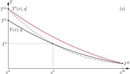
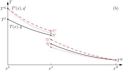
Figure 2: A schematic example of temperature profiles of systems (a) without any junctions and (b) with a single junction at $x^{J}$ when the temperature at $x^{R}$ is fixed and the temperature at $x^{L}$ is increased from $T^{L}$ to $T^{\prime L}$. The dotted lines in (b) would give rise to NDTC.

Systems with a single abrupt junction, as shown in Fig. 1(b). We assume that the abrupt junction is located at $x^{J}\in(x^{L},x^{R})$. The system can be considered as two subsystems without any abrupt junctions coupled together at $x^{J}$. We suppose that the subsystems in $[x^{L},x^{J}]$ and $[x^{J},x^{R}]$ have thermal conductivity $\kappa_{1}(x,T_{1})$ with temperature profile $T_{1}(x)$ and $\kappa_{2}(x,T_{2})$ with temperature profile $T_{2}(x)$ respectively. We denote

$$T_{1}^{J}\equiv T_{1}(x^{J}),\;T_{2}^{J}\equiv T_{2}(x^{J}),$$ (8)

$$T^{L}\equiv T_{1}(x^{L}),\;T^{R}\equiv T_{2}(x^{R}).$$

At the junction, the two subsystems are coupled through a thermal contact resistance (TCR) $R^{J}$, defined such that the heat current $q$ flowing through the system satisfies not (b)

$$T_{1}^{J}-T_{2}^{J}=qR^{J}(T_{1}^{J},T_{2}^{J}).$$ (9)

We have generally assumed that the TCR depend on two temperatures $T_{1}^{J}$ and $T_{2}^{J}$. The TCR $R^{J}(T_{1}^{J},T_{2}^{J})$ provides the complete characterizations of the junction at the phenomenological level.

The possibility of NDTC here can also be interpreted graphically. Again, take the case that $T^{R}$ is fixed as an example. If the temperature $T^{L}$ ($>T^{R}$) is increased to $T^{\prime L}$ ($>T^{L}$), the temperature profile $T(x)$ with $T(x^{L(R)})=T^{L(R)}$, junction temperatures $T_{1,2}^{J}$ and heat current $q$ are changed to $T^{\prime}(x)$ with $T^{\prime}(x^{L})=T^{\prime L}$ and $T^{\prime}(x^{R})=T^{R}$, junction temperatures $T_{1,2}^{\prime J}$ and heat current $q^{\prime}$, as illustrated in Fig. 2(b). Because of the discontinuous jump of temperature at $x^{J}$, we could have $q^{\prime}>q$ if $T_{2}^{\prime J}>T_{2}^{J}$ (red dashed line) or $q^{\prime}<q$ if $T_{2}^{\prime J}<T_{2}^{J}$ (red dotted line) where the latter situation gives rise to NDTC. We derive the conditions of the existence of NDTC in more detail below.

Analytically, the DTCs are (Appendix B)

$$G^{L}\!\!=\!\!\left(\!1\!-\!q\frac{\partial R^{J}}{\partial T_{1}^{J}}\!\right)\!\!\frac{F_{1}(x^{L})}{R^{D}},G^{R}\!\!=\!\!\left(\!1\!+\!q\frac{\partial R^{J}}{\partial T_{2}^{J}}\!\right)\!\!\frac{F_{2}(x^{R})}{R^{D}},$$ (10)

with

$$F_{i}(x)\!\equiv\!\exp\!\!\left(\int_{x^{J}}^{x}\!\frac{1}{\kappa_{i}(x^{\prime}\!,T_{i}(x^{\prime}))}\frac{\partial\kappa_{i}}{\partial T_{i}}\frac{\mathrm{d}T_{i}}{\mathrm{d}x^{\prime}}\mathrm{d}x^{\prime}\!\right)\!,i\!=\!1,2,$$ (11)

defined on $[x^{L},x^{J}]$ and $[x^{J},x^{R}]$ respectively, and

$$R^{D}\equiv R^{J}+\displaystyle\left(1-q\frac{\partial R^{J}}{\partial T_{1}^{J}}\right)J_{1}+\left(1+q\frac{\partial R^{J}}{\partial T_{2}^{J}}\right)J_{2}$$ (12)

where

$$J_{1}\!\!\equiv\!\!\!\int_{x^{L}}^{x^{J}}\!\!\!\frac{F_{1}(x^{\prime})}{\kappa_{1}\!(x^{\prime}\!,T_{1}\!(x^{\prime}))}\mathrm{d}x^{\prime},J_{2}\!\!\equiv\!\!\!\int_{x^{J}}^{x^{R}}\!\!\!\frac{F_{2}(x^{\prime})}{\kappa_{2}\!(x^{\prime}\!,T_{2}\!(x^{\prime}))}\mathrm{d}x^{\prime}.$$ (13)

If the TCR is independent of the junction temperatures $T_{1}^{J}$ and $T_{2}^{J}$, the partial derivatives of $R^{J}$ in Eqs. (10) and (12) vanishes, and since $F_{i}$ in Eq. (11) and $J_{i}$ in Eq. (13) are positive, thus $G^{L(R)}>0$ and there is no NDTC. Therefore, a temperature dependent TCR is necessary for the existence of NDTC. However, as we will see, it is not a sufficient condition.

In the presence of the temperature dependence of TCR, we pick a $T_{B}$ such that $T_{B}^{-1}>|R^{-1}\partial R^{J}/\partial T_{1,2}^{J}|$, where $R=(T^{L}-T^{R})/q$ is the thermal resistance of the whole system including the TCR. Inside the regime defined by $|T^{L}-T^{R}|<T_{B}$ in the $(T^{L},T^{R})$ quarter plane we have $|q\partial R^{J}/\partial T^{J}_{1,2}|<1$ and subsequently $R^{D}>0$ and $G^{L(R)}>0$: no NDTC is displayed in this low bias regime. Therefore, a temperature bias exceeding $T_{B}$ is required to observe NDTC, confirming that NDTC is a nonlinear thermal transport phenomenon.

As the temperature bias ($|T^{L}-T^{R}|$) increases beyond $T_{B}$, $G^{L(R)}$ could possibly be negative, leading to NDTC. We denote the dimensionless quantities

$$X\equiv\left(1-q\frac{\partial R^{J}}{\partial T_{1}^{J}}\right)\frac{J_{1}}{R^{J}}=\frac{\partial q}{\partial T_{1}^{J}}J_{1},$$ (14)

$$Y\equiv\left(1+q\frac{\partial R^{J}}{\partial T_{2}^{J}}\right)\frac{J_{2}}{R^{J}}=-\frac{\partial q}{\partial T_{2}^{J}}J_{2}$$

such that

$$G^{L}=\frac{X}{1\!+\!X\!+\!Y}\frac{F_{1}(x^{L})}{J_{1}},G^{R}=\frac{Y}{1\!+\!X\!+\!Y}\frac{F_{2}(x^{R})}{J_{2}}.$$ (15)

Now there exists NDTC if and only if at least one of $X$ and $Y$ is negative, which means that at least one of $\partial q/\partial T_{1}^{J}$ and $-\partial q/\partial T_{2}^{J}$ is negative not (c). We refer to such junctions as those with intrinsic junction NDTC which is now necessary and sufficient for NDTC to occur. Thus, the existence of NDTC in systems with a single abrupt junction is uniquely determined by the properties of the TCRs, regardless of the properties of the system away from the junction.

Furthermore, we can formulate the existence of NDTC on the $X$-$Y$ plane: find out the points on the plane that correspond to negative $G^{L}$ or $G^{R}$. NDTC exists inside the shaded areas (A, B and C in Fig. 3), not including the boundaries labelled by the thick solid black and red dashed lines. Note that we have $G^{L}<0$ and $G^{R}=0$ on the thin dotted line ($-1<X<0$, $Y=0$) while $G^{L}=0$ and $G^{R}<0$ on the thin dash-dotted line ($X=0$, $-1<Y<0$). We have $R^{D}=0$ and thus infinite ($\pm\infty$) DTCs on the thick red dashed line not (d). For the points in the shaded areas and close to the thick red dashed line, we can have very large magnitude of NDTC, useful to design sensitive detectors for temperature fluctuations.

Figure 3: The phase diagram on the $X-Y$ plane that present NDTC.

The blue and cyan shaded areas A and B in Fig. 3 are not bounded on the $X$-$Y$ plane. They correspond to one of $G^{L}$ and $G^{R}$ is negative and the other is positive, i.e., $G^{L}G^{R}<0$ which is equivalent to

$$XY<0.$$ (16)

Eq. (16) includes the situation that $G^{L(R)}$ is infinite (on the thick solid red lines inside the second and the fourth quarters of the $X$-$Y$ plane). We can write Eq. (16) in a more transparent way by rewriting the temperature dependence of the TCR $R^{J}(T_{1}^{J},T_{2}^{J})=R^{J}(\hat{T}^{J},\bar{T}^{J})$ where $\hat{T}^{J}\equiv T_{1}^{J}-T_{2}^{J}$ and $\bar{T}^{J}\equiv T_{1}^{J}+T_{2}^{J}$:

$$\left|q\frac{\partial R^{J}}{\partial\hat{T}^{J}}-1\right|<\left|q\frac{\partial R^{J}}{\partial\bar{T}^{J}}\right|.$$ (17)

Eqs. (17) implies that $\left|q\frac{\partial R^{J}}{\partial\bar{T}^{J}}\right|>0$, i.e., the TCR must be dependent on $\bar{T}^{J}$. This is physically significant, because in thermal transport we have a natural temperature ground of absolute zero temperature. This demonstrates the drastic difference between the thermal and electrical transport, where in the latter case the junction behaviour only depends on the voltage difference (not the average voltage) across the junction.

The red shaded area C in Fig. 3 is bounded and it corresponds to the case that both $1-q\partial R^{J}/\partial T^{J}_{1}$ and $1+q\partial R^{J}/\partial T^{J}_{2}$ are negative and $R^{D}$ is positive, equivalent to

$$q\frac{\partial R^{J}}{\partial\hat{T}^{J}}-1>\left|q\frac{\partial R^{J}}{\partial\bar{T}^{J}}\right|,|q|<\frac{R^{J}+J_{1}+J_{2}}{\left|\frac{\partial R^{J}}{\partial T_{1}^{J}}\right|J_{1}+\left|\frac{\partial R^{J}}{\partial T_{2}^{J}}\right|J_{2}}.$$ (18)

Eq. (17) and Eq. (18) imply that

$$|q|>\left(\text{max}\left\{\left|\frac{\partial R^{J}}{\partial T_{1}^{J}}\right|,\left|\frac{\partial R^{J}}{\partial T_{2}^{J}}\right|\right\}\right)^{-1}$$ (19)

and

$$|q|>\left(\text{min}\left\{\left|\frac{\partial R^{J}}{\partial T_{1}^{J}}\right|,\left|\frac{\partial R^{J}}{\partial T_{2}^{J}}\right|\right\}\right)^{-1}$$ (20)

respectively, suggesting a positive minimum on the heat current for the existence of NDTC. This again indicates that the existence of NDTC is in the nonlinear regime, beyond low heat current.

At the onset of NDTC, we have either $G^{L}=0$ or $G^{R}=0$ and the magnitude of heat current (vs. temperature bias) reaches its local maximum. Taking the case of $G^{L}=0$ as an example, we have the following variation rates at the vicinity of $G^{L}=0$ (Appendix B):

$$\frac{\delta(T_{1}^{J}-T_{2}^{J})}{\delta T^{L}}\!=\!F_{1}(x^{L})\!-\!G^{L}(J_{1}\!+\!J_{2})\!\approx\!F_{1}(x^{L})>0,$$ (21)

$$\frac{\delta(T_{2}^{J}-T^{R})}{\delta T^{L}}=G^{L}J_{2}.$$

When the system enters the NDTC regime of $G^{L}\lesssim 0$, the temperature increase $\delta T^{L}$ of $T^{L}$ is distributed over $[x^{L},x^{R}]$ in such a way that the temperature drop over $[x^{J},x^{R}]$ is decreasing with increasing $T^{L}$ (which is the manifestation of NDTC) while the temperature drop over the junction is increasing with $T^{L}$, as shown in Fig. 2.

Systems with multiple abrupt junctions can exhibit both NDTC and infinite DTCs, but the detailed conditions for their occurrence are more complicated. It can be proved that NDTC still requires that at least one of the junctions possess intrinsic junction NDTC (Appendix C). Nevertheless, these junctions can be grouped into a single effective junction with its properties determined by the way the junctions are organized (e.g., the order and the connection materials) and by the properties of those individual junctions, as shown in Fig. 1(c). After identifying the effective TCR $R^{J}_{\text{eff}}$, we can treat the system with multiple junctions as one with a single junction. The discussions in the previous section can be readily applied by simply replacing $R^{J}$ with $R^{J}_{\text{eff}}$.

This procedure also provides us a routine to engineer the TCR. For example, we can construct a system composed of three segments in $[x^{L},x_{1}^{J}]$, $[x_{1}^{J},x_{2}^{J}]$ and $[x_{2}^{J},x^{R}]$. Suppose that $[x^{L},x_{1}^{J}]$ and $[x_{2}^{J},x^{R}]$ contain the same kind of uniform material and the material in $[x_{1}^{J},x_{2}^{J}]$ is also uniform but different. We can have a single effective junction with its TCR $R^{J}_{\text{eff}}=q/(T_{1}^{J}-T_{2}^{J})$ where $T_{1}^{J}$ is the temperature at $x_{1}^{J}$ at the side of $[x^{L},x_{1}^{J}]$, $T_{2}^{J}$ is the temperature at $x_{2}^{J}$ at the side of $[x_{2}^{J},x^{R}]$ and $q$ is the heat current flowing across the effective junction. In this way, we have a symmetrical effective junction, i.e., $R^{J}_{\text{eff}}(T_{1}^{J},T_{2}^{J})=R^{J}_{\text{eff}}(T_{2}^{J},T_{1}^{J})$.

In conclusion, we have studied the steady state 1D thermal transport in the diffusive regime without heat sources or sinks. The Fourier’s law is applied to calculate the differential thermal conductance. We find that NDTC (in the case that the temperature at one end is fixed) cannot exist in systems without any abrupt thermal junctions. However, we could have NDTC if and only if a junction with intrinsic junction NDTC is introduced. Our predictions provide a theoretical foundation to experimentally realize NDTC through careful thermal contact engineering, though it remains an open question to realize a junction with intrinsic junction NDTC.

This work is partially supported by the Semiconductor Research Corporation (SRC) - Nanoelectronics Research Initiative (NRI) via Midwest Institute for Nanoelectronics Discovery (MIND) and the Cooling Technologies Research Center (CTRC) at Purdue University. JH thanks Prof. Xiulin Ruan (Purdue University) and Dr. Xingpeng Yan for useful discussions.

Appendix

.1 Systems without abrupt junctions

To calculate the differential thermal conductance (DTC), we start from the variation of $q=-\kappa(x,T(x))\frac{\mathrm{d}T(x)}{\mathrm{d}x}$:

$$\delta q=-\kappa(x,T)\frac{d}{dx}\delta T-\frac{\partial\kappa}{\partial T}\frac{\mathrm{d}T}{\mathrm{d}x}\delta T.$$ (22)

We define

$$U^{L(R)}(x)\equiv\frac{\delta T(x)}{\delta T^{L(R)}}$$ (23)

which according to Eq. (22) satisfies

$$\frac{\mathrm{d}}{\mathrm{d}x}U^{L(R)}+\frac{1}{\kappa(x,T)}\frac{\partial\kappa}{\partial T}\frac{\mathrm{d}T}{\mathrm{d}x}U^{L(R)}+\frac{\eta^{L(R)}G^{L(R)}}{\kappa(x,T)}=0.$$ (24)

where $\eta^{L}=1$ and $\eta^{R}=-1$. At the boundaries we have

$$\delta T(x^{L(R)})=\delta T^{L(R)}\;\;\text{while}\;\;\delta T(x^{R(L)})=0,$$ (25)

since $T(x^{L(R)})=T^{L(R)}$. Thus from Eq. (23), the boundary conditions for Eq. (24) are

$$U^{L}(x^{L})=1,U^{L}(x^{R})=U^{R}(x^{L})=0,U^{R}(x^{R})=1.$$ (26)

Eq. (24) is an inhomogeneous linear ordinary differential equation, and the coefficients $\frac{1}{\kappa(x,T)}\frac{\partial\kappa}{\partial T}\frac{\mathrm{d}T}{\mathrm{d}x}$ and $\frac{\eta^{L(R)}G^{L(R)}}{\kappa(x,T)}$ are functions of $x$ only, since $T(x)$ is already formally solved from Eq. (2) and boundary conditions Eq. (3). The solution to Eq. (24) is

$${U^{L\!(R)}(x)\!\!=\!\!\frac{U^{L\!(R)}(x^{L})}{F(x)}\!\!-\!\!\frac{\eta^{L\!(R)}G^{L\!(R)}}{F(x)}\!\!\int_{x^{L}}^{x}\!\frac{F(x^{\prime})}{\kappa(x^{\prime},T(x^{\prime}))}\mathrm{d}x^{\prime},}$$ (27)

where

$$F(x)\equiv\exp\left(\int_{x^{L}}^{x}\frac{1}{\kappa(x^{\prime},T(x^{\prime}))}\frac{\partial\kappa}{\partial T}\frac{\mathrm{d}T}{\mathrm{d}x^{\prime}}\mathrm{d}x^{\prime}\right).$$ (28)

By evaluating Eq. (27) at $x=x^{R}$, we obtain

$$G^{L(R)}=J^{-1}\eta^{L(R)}\left[U^{L(R)}(x^{L})-F(x^{R})U^{L(R)}(x^{R})\right],$$ (29)

where

$$J\equiv\int_{x^{L}}^{x^{R}}\frac{F(x^{\prime})}{\kappa(x^{\prime},T(x^{\prime}))}\mathrm{d}x^{\prime}.$$ (30)

From Eq. (26) and Eq. (29), we have

$$G^{L}=J^{-1},\;\;G^{R}=F(x^{R})J^{-1}.$$ (31)

.2 Systems with a single junction

For a system composed of two segments lying in $[x^{L},x^{J}]$ and $[x^{J},x^{R}]$, we denote the temperature profiles $T_{1}(x)$ and $T_{2}(x)$ and the thermal conductivity $\kappa_{1}(x,T_{1}(x))$ and $\kappa_{2}(x,T_{1}(x))$, receptively. If a heat current is flowing in the system, the temperature profiles satisfy

$$q=-\kappa_{1}(x,T_{1}(x))\frac{\mathrm{d}T_{1}}{\mathrm{d}x},\;\;\;\;x^{L}<x<x^{J},$$ (32)

$$q=-\kappa_{2}(x,T_{2}(x))\frac{\mathrm{d}T_{2}}{\mathrm{d}x},\;\;\;\;x^{J}<x<x^{R}$$

with the boundary conditions

$$T_{1}^{J}-T_{2}^{J}=qR^{J}(T_{1}^{J},T_{2}^{J}),T_{1}(x^{L})=T^{L},T_{2}(x^{R})=T^{R}.$$ (33)

Applying the variation $\delta T^{L(R)}$ of the boundary temperature at one end, the resulting temperature profiles $T_{1}$ and $T_{2}$ are varied to $T_{1}(x)+\delta T_{1}(x)$ and $T_{2}(x)+\delta T_{2}(x)$ respectively. Of course we have

$$\delta T_{1}(x^{L})=\delta T^{L},\;\;\delta T_{2}(x^{R})=\delta T^{R}.$$ (34)

The heat current $q$ is varied to $q+\delta q$. The junction temperatures $T_{1}^{J}$ and $T_{2}^{J}$ are varied to $T_{1}^{J}+\delta T_{1}^{J}$ and $T_{2}^{J}+\delta T_{2}^{J}$ respectively. We then define the following functions

$$U_{1}^{L(R)}\equiv\frac{\delta T_{1}}{\delta T^{L(R)}}\;\;\text{and}\;\;U_{2}^{L(R)}\equiv\frac{\delta T_{2}}{\delta T^{L(R)}}$$ (35)

on $[x^{L},x^{J}]$ and $[x^{J},x^{R}]$, respectively. They satisfy the following equations

$$\eta^{\!L\!(R)}\!G^{L\!(R)}\!=\!-\kappa_{i}\!\frac{\mathrm{d}U_{i}^{L\!(R)}}{\mathrm{d}x}\!-\!\frac{\partial\kappa_{i}}{\partial T_{i}}\!\frac{\mathrm{d}T_{i}}{\mathrm{d}x}U_{i}^{L\!(R)},\;i=1,2$$ (36)

and boundary conditions

$$U_{1}^{L}(x^{L})=1,U_{1}^{R}(x^{L})=U_{2}^{L}(x^{R})=0,U_{2}^{R}(x^{R})=1.$$ (37)

Their solutions are

$$U_{i}^{L\!(R)}\!(x)\!\!=\!\!\frac{U_{i}^{L\!(R)}\!(x^{J})}{F_{i}(x)}\!-\!\frac{\eta^{L\!(R)}G^{L\!(R)}}{F_{i}(x)}\!\!\int_{x^{J}}^{x}\frac{F_{i}(x^{\prime})}{\kappa_{i}(x^{\prime},T_{i}(x^{\prime}))}\mathrm{d}x^{\prime}$$ (38)

where

$$F_{i}(x)\!\equiv\!\exp\!\left(\int_{x^{J}}^{x}\frac{1}{\kappa_{i}(x^{\prime},T_{i}(x^{\prime}))}\frac{\partial\kappa_{i}}{\partial T_{i}}\frac{\mathrm{d}T_{i}}{\mathrm{d}x^{\prime}}\mathrm{d}x^{\prime}\!\right),\;i=1,2.$$ (39)

By evaluating Eq. (38) at $x^{L}$ for $i=1$ and at $x^{R}$ for $i=2$, we have

$$U_{1}^{L(R)}(x^{J})= F_{1}(x^{L})U_{1}^{L(R)}(x^{L})$$ (40)

$$+\eta^{L\!(R)}G^{L\!(R)}\int_{x^{J}}^{x^{L}}\frac{F_{1}(x^{\prime})}{\kappa_{1}(x^{\prime},T_{1}(x^{\prime}))}\mathrm{d}x^{\prime},$$

$$U_{2}^{L(R)}(x^{J})= F_{2}(x^{R})U_{2}^{L(R)}(x^{R})$$

$$+\eta^{L\!(R)}G^{L\!(R)}\int_{x^{J}}^{x^{R}}\frac{F_{2}(x^{\prime})}{\kappa_{2}(x^{\prime},T_{2}(x^{\prime}))}\mathrm{d}x^{\prime}.$$

The variation of the first equation in Eq. (33) gives

$$U_{1}^{L(R)} (x^{J})-U_{2}^{L(R)}(x^{J})=\eta^{L(R)}G^{L(R)}R^{J}$$ (41)

$$+q\frac{\partial R^{J}}{\partial T_{1}^{J}}U_{1}^{L(R)}(x^{J})+q\frac{\partial R^{J}}{\partial T_{2}^{J}}U_{2}^{L(R)}(x^{J}).$$

By inserting Eq. (40) into Eq. (41), we finally get the DTC

$$G^{L}=\left(1-q\frac{\partial R^{J}}{\partial T_{1}^{J}}\right)\frac{F_{1}(x^{L})}{R^{D}},$$ (42)

$$G^{R}=\left(1+q\frac{\partial R^{J}}{\partial T_{2}^{J}}\right)\frac{F_{2}(x^{R})}{R^{D}},$$

where

$$R^{D}\equiv R^{J}+\left(1-q\frac{\partial R^{J}}{\partial T_{1}^{J}}\right)J_{1}+\left(1+q\frac{\partial R^{J}}{\partial T_{2}^{J}}\right)J_{2},$$ (43)

with

$$J_{1}\!\!\equiv\!\!\!\int_{x^{L}}^{x^{J}}\!\!\!\frac{F_{1}(x^{\prime})}{\kappa_{1}\!(x^{\prime}\!,T_{1}\!(x^{\prime}))}\mathrm{d}x^{\prime},J_{2}\!\!\equiv\!\!\!\int_{x^{J}}^{x^{R}}\!\!\!\frac{F_{2}(x^{\prime})}{\kappa_{2}\!(x^{\prime}\!,T_{2}\!(x^{\prime}))}\mathrm{d}x^{\prime}.$$ (44)

From Eq. (40), we can also readily write down

$$\frac{\delta(T_{1}^{J}-T_{2}^{J})}{\delta T^{L}} =U_{1}^{L}(x^{J})-U_{2}^{L}(x^{J})$$ (45)

$$=F_{1}(x^{L})-G^{L}(J_{1}+J_{2}),$$

$$\frac{\delta(T_{2}^{J}-T^{R})}{\delta T^{L}} =U_{2}^{L}(x^{J})=G^{L}J_{2}.$$

.3 Existence of NDTC for systems with multiple junctions

To prove that the existence of NDTC for systems with multiple junctions requires that at least one of the junctions has intrinsic junction NDTC, we prove the converse by induction, i.e., there is no NDTC if none of the junctions has intrinsic junction NDTC.

Assume that the system lying in $[x^{J},x^{R}]$ contains an arbitrary number of junctions and the DTCs for this system are non-negative. We now add a new segment (with no junctions within the segment) lying in $[x^{L},x^{J}]$ to the existing system. We denote $T^{L(R)}$ as the temperature at $x^{L(R)}$. We assume that the new junction at $x^{J}$ with TCR $R^{J}(T_{1}^{J},T_{2}^{J})$ has no intrinsic junction NDTC. Here $T_{1}^{J}$ and $T_{2}^{J}$ are the temperatures at $x^{J}$ at the side of $[x^{L},x^{J}]$ and $[x^{J},x^{R}]$ respectively. Suppose we raise the temperature $T^{L}$ infinitesimally to $T^{L}+\delta T^{L}$ ($\delta T^{L}>0$) while keeping $T^{R}$ fixed. The temperature $T_{1(2)}^{J}$ is then varied to $T_{1(2)}^{J}+\delta T_{1(2)}^{J}$ and the heat current is changed from $q$ to $q+\delta q$. At the junction, we have $\delta q=G_{1}^{J}\delta T_{1}^{J}-G_{2}^{J}\delta T_{2}^{J}$ where $G_{1(2)}^{J}\geq 0$ are the junction DTCs. On the other hand, the system in $[x^{J},x^{R}]$ has non-negative DTCs, i.e., $\delta q=G^{B}\delta T_{2}^{J}$ where $G^{B}\geq 0$. We thus have $G_{1}^{J}\delta T_{1}^{J}=(G_{2}^{J}+G^{B})\delta T_{2}^{J}$. Of course $\delta T_{1}^{J}$ cannot be negative. If either $G_{2}^{J}$ or $G^{B}$ is positive, we will have $\delta T_{2}^{J}=G_{1}^{J}\delta T_{1}^{J}/(G_{2}^{J}+G^{B})\geq 0$ and thus $\delta q=G^{B}\delta T_{2}^{J}\geq 0$ and there is no NDTC. If both $G_{2}^{J}$ and $G^{B}$ are zero, we will have $\delta q=G_{1}^{J}\delta T_{1}^{J}\geq 0$ and there is no NDTC.

References

• Lepri et al. (2003) S. Lepri, R. Livi,  and A. Politi, Phys. Rep. 377, 1 (2003).
• Li et al. (2012) N. Li, J. Ren, L. Wang, G. Zhang, P. Hänggi,  and B. Li, Rev. Mod. Phys. 84, 1045 (2012).
• Terraneo et al. (2002) M. Terraneo, M. Peyrard,  and G. Casati, Phys. Rev. Lett. 88, 094302 (2002).
• Eckmann and Mejía-Monasterio (2006) J.-P. Eckmann and C. Mejía-Monasterio, Phys. Rev. Lett. 97, 094301 (2006).
• Li et al. (2004) B. Li, L. Wang,  and G. Casati, Phys. Rev. Lett. 93, 184301 (2004).
• Casati et al. (2007) G. Casati, C. Mejía-Monasterio,  and T. Prosen, Phys. Rev. Lett. 98, 104302 (2007).
• Peyrard (2006) M. Peyrard, Europhysics Lett. 76, 49 (2006).
• Chang et al. (2006) C. W. Chang, D. Okawa, A. Majumdar,  and A. Zettl, Science 314, 1121 (2006).
• Yang et al. (2007) N. Yang, N. Li, L. Wang,  and B. Li, Phys. Rev. B 76, 020301 (2007).
• Hu et al. (2009) J. Hu, X. Ruan,  and Y. P. Chen, Nano Lett. 9, 2730 (2009).
• Pereira (2010) E. Pereira, Phys. Rev. E 82, 040101 (2010).
• Sawaki et al. (2011) D. Sawaki, W. Kobayashi, Y. Moritomo,  and I. Terasaki, Appl. Phys. Lett. 98, 081915 (2011).
• Go and Sen (2010) D. B. Go and M. Sen, J. Heat Transfer 132, 124502 (2010).
• Dames (2009) C. Dames, J. Heat Transfer 131, 061301 (2009).
• Li et al. (2006) B. Li, L. Wang,  and G. Casati, Appl. Phys. Lett. 88, 143501 (2006).
• Wang and Li (2007) L. Wang and B. Li, Phys. Rev. Lett. 99, 177208 (2007).
• He et al. (2009) D. He, S. Buyukdagli,  and B. Hu, Phys. Rev. B 80, 104302 (2009).
• Zhong et al. (2009) W.-R. Zhong, P. Yang, B.-Q. Ai, Z.-G. Shao,  and B. Hu, Phys. Rev. E 79, 050103 (2009).
• Shao et al. (2009) Z.-G. Shao, L. Yang, H.-K. Chan,  and B. Hu, Phys. Rev. E 79, 061119 (2009).
• He et al. (2010) D. He, B.-Q. Ai, H.-K. Chan,  and B. Hu, Phys. Rev. E 81, 041131 (2010).
• Ai and Hu (2011) B.-Q. Ai and B. Hu, Phys. Rev. E 83, 011131 (2011).
• Ai et al. (2011) B.-Q. Ai, W.-R. Zhong,  and B. Hu, Phys. Rev. E 83, 052102 (2011).
• Hu et al. (2011) J. Hu, Y. Wang, A. Vallabhaneni, X. Ruan,  and Y. P. Chen, Appl. Phys. Lett. 99, 113101 (2011).
• Shao and Yang (2011) Z.-G. Shao and L. Yang, Europhysics Lett. 94, 34004 (2011).
• Zhu et al. (2012) L. Zhu, C. R. Otey,  and S. Fan, Appl. Phys. Lett. 100, 044104 (2012).
• Segal (2006) D. Segal, Phys. Rev. B 73, 205415 (2006).
• Wu et al. (2009) L.-A. Wu, C. X. Yu,  and D. Segal, Phys. Rev. E 80, 041103 (2009).
• Walter and Thompson (1998) W. Walter and R. Thompson, Ordinary Differential Equations (Springer, 1998).
• not (a) If the temperatures at both ends vary simultaneously and depend on a parameter $u$ (i.e., $T^{L(R)}(u)$), the DTC is $G=\frac{G^{L}dT^{L}/du-G^{R}dT^{R}/du}{dT^{L}/du-dT^{R}/du}$. It is possible to have the numerator of $G$ to be negative while its denominator is positive, if the form of $T^{L(R)}(u)$ is designed carefully.
• not (b) Usually $R^{J}(T_{1}^{J},T_{2}^{J})$ is reduced to $R^{J}(T^{J})$ with $T^{J}=(T_{1}^{J}+T_{2}^{J})/2$ when $|T_{1}^{J}-T_{2}^{J}|\ll T^{J}$, as being studied in many experiments (E. T. Swartz and R. O. Pohl, Rev. Mod. Phys. 61, 605 (1989)). However, that form of $R^{J}$ is not applicable to the cases involving large currents that we are particularly interested in here.
• not (c) To have NDTC (negative $G^{L}$ or $G^{R}$), it is necessary that at least one of $X$ and $Y$ is negative. Conversely, if at least one of $X$ and $Y$ is negative, since both $X$ and $Y$ (assumed to be continuous with temperature bias) would be positive in the limit of vanishing temperature bias, there exists a critical temperature bias below which both $X$ and $Y$ are positive and slightly above which at least one of $X$ and $Y$ is negative and $|X|\ll 1$ and $|Y|\ll 1$, thus one of $G^{L}$ and $G^{R}$ must be negative ($1+X+Y$ is positive) and there exists NDTC.
• not (d) The zeros of $G^{L}$ and $G^{R}$ exist at $q=[\partial R^{J}/\partial T_{1}^{J}]^{-1}$ and $q=-[\partial R^{J}/\partial T_{2}^{J}]^{-1}$ respectively. The zeros may accidentally cancel the singularity at $(X,Y)=(0,-1)$ or $(X,Y)=(-1,0)$, but this cancellation rarely happen, and can be avoided by slightly perturbing the boundary temperatures.