SparseDTW: A Novel Approach to Speed up Dynamic Time Warping

Abstract

We present a new space-efficient approach, (SparseDTW), to compute the Dynamic Time Warping (DTW) distance between two time series that always yields the optimal result. This is in contrast to other known approaches which typically sacrifice optimality to attain space efficiency. The main idea behind our approach is to dynamically exploit the existence of similarity and/or correlation between the time series. The more the similarity between the time series the less space required to compute the DTW between them. To the best of our knowledge, all other techniques to speedup DTW, impose apriori constraints and do not exploit similarity characteristics that may be present in the data. We conduct experiments and demonstrate that SparseDTW outperforms previous approaches.

Keywords: Time series, Similarity measures, Dynamic time warping, Data mining

1 Introduction

Dynamic time warping (DTW) uses the dynamic programming paradigm to compute the alignment between two time series. An alignment “warps” one time series onto another and can be used as a basis to determine the similarity between the time series. DTW has similarities to sequence alignment in bioinformatics and computational linguistics except that the matching process in sequence alignment and warping have to satisfy a different set of constraints and there is no gap condition in warping. DTW first became popular in the speech recognition community (Sakoe & Chiba, 1978) where it has been used to determine if the two speech wave-forms represent the same underlying spoken phrase. Since then it has been adopted in many other diverse areas and has become the similarity metric of choice in time series analysis (Keogh & Pazzani, 2000).

Like in sequence alignment, the standard DTW algorithm has $O(mn)$ space complexity where $m$ and $n$ are the lengths of the two sequences being aligned. This limits the practicality of the algorithm in todays “data rich environment” where long sequences are often the norm rather than the exception. For example, consider two time series which represent stock prices at one second granularity. A typical stock is traded for at least eight hours on the stock exchange and that corresponds to a length of $8\times 60\times 60=28800$. To compute the similarity, DTW would have to store a matrix with at least 800 million entries!

Figure 1(a) shows an example of an alignment (warping) between two sequences $S$ and $Q$. It is clear that there are several possible alignments but the challenge is to select the one which has the minimal overall distance. The alignment has to satisfy several constraints which we will elaborate on in Section 3.

Salvador & Chan (2007) have provided a succinct categorization of different techniques that have been used to speed up DTW:

• Constraints: By adding additional constraints the search space of possible alignments can be reduced. Two well known exemplars of this approach are the Sakoe & Chiba (1978) and the Itakura (1975) constraints which limit how far the alignment can deviate from the diagonal. While these approaches provide a relief in the space complexity, they do not guarantee the optimality of the alignment.

• Data Abstraction: In this approach, the warping path is computed at a lower resolution of the data and then mapped back to the original resolution (Salvador & Chan, 2007). Again, optimality of the alignment is not guaranteed.

• Indexing: Keogh & Ratanamahatana (2004), Sakurai et al. (2005), and Lemire (2009) proposed an indexing approach, which does not directly speed up DTW but limits the number of DTW computations. For example, suppose there exists a database D of time series sequences and a query sequence $q$. We want to retrieve all sequences $d\in D$ such that $DTW(q,d)<\epsilon$. Then instead of checking $q$ against each and every sequence in $D$, an easy to calculate lower bound function LBF is first applied between $q$ and $D$. The argument works as follows:

  1. By construction, $LBF(q,d)<DTW(q,d)$.

  2. Therefore, if $LBF(q,d)>\epsilon$ then $DTW(q,d)>\epsilon$ and $DTW(q,d)$ does not have to be computed.

1.1 Main Contribution

The main insight behind our proposed approach, SparseDTW, is to dynamically exploit the possible existence of inherent similarity and correlation between the two time series whose DTW is being computed. This is the motivation behind the Sakoe-Chiba band and the Itakura Parellelogram but our approach has three distinct advantages:

1. Bands in SparseDTW evolve dynamically and are, on average, much smaller than the traditional approaches. We always represent the warping matrix using sparse matrices, which leads to better average space complexity compared to other approaches (Figure 9(c)).

2. SparseDTW always yields the optimal warping path since we never have to set apriori constraints independently of the data. For example, in the traditional banded approaches, a sub-optimal path will result if all the possible optimal warping paths have to cross the bands.

3. Since SparseDTW yields an optimal alignment, it can easily be used in conjunction with lower bound approaches.

1.2 Paper Outline

The rest of the paper is organized as follows: Section 2 describes related work on DTW. The DTW algorithm is described in Section 3. In Section 4, we give an overview of the techniques used to speed up DTW by adding constraints. Section 5 reviews the Divide and Conquer approach for DTW which is guaranteed to take up $O(m+n)$ space and $O(mn)$ time. Furthermore, we provide an example which clearly shows that the divide and conquer approach fails to arrive at the optimal DTW result. The SparseDTW algorithm is introduced with a detailed example in Section 6. We analyze and discuss our results in Section 7, followed by our conclusions in Section 8.

2 Related Work

DTW was first introduced in the data mining community in the context of mining time series (Berndt & Clifford, 1994). Since it is a flexible measure for time series similarity it is used extensively for ECGs (Electrocardiograms) (Caiani et al., 1998), speech processing (Rabiner & Juang, 1993), and robotics (Schmill et al., 1999). It is important to know that DTW is a measure not a metric, because DTW does not satisfy the triangular inequality.

Several techniques have been introduced to speed up DTW and/or reduce the space overhead (Hirschberg, 1975; Yi et al., 1998; Kim et al., 2001; Keogh & Ratanamahatana, 2004; Lemire, 2009).

Divide and conquer (DC) heuristic proposed by Hirschberg (1975); that is a dynamic programming algorithm that finds the least cost sequence alignment between two strings in linear space and quadratic time. The algorithm was first used in speech recognition area to solve the Longest Common Subsequence (LCSS). However as we will show with the help of an example, DC does not guarantee the optimality of the DTW distance.

Sakoe & Chiba (1978) speed up the DTW by constraining the warping path to lie within a band around the diagonal. However, if the optimal path crosses the band, the result will not be optimal.

Keogh & Ratanamahatana (2004) and Lemire (2009) introduced efficient lower bounds that reduce the number of DTW computations in a time series database context. However, these lower bounds do not reduce the space complexity of the DTW computation, which is the objective of our work.

Sakurai et al. (2005) presented FTW, a search method for DTW; it adds no global constraints on DTW. Their method designed based on a lower bounding distance measure that approximates the DTW distance. Therefore, it minimizes the number of DTW computations but does not increase the speed the DTW itself.

Salvador & Chan (2007) introduced an approximation algorithm for DTW called FastDTW. Their algorithm begins by using DTW in very low resolution, and progresses to a higher resolution linearly in space and time. FastDTW is performed in three steps: coarsening shrinks the time series into a smaller time series; the time series is projected by finding the minimum distance (warping path) in the lower resolution; and the warping path is an initial step for higher resolutions. The authors refined the warping path using local adjustment. FastDTW is an approximation algorithm, and thus there is no guarantee it will always find the optimal path. It requires the coarsening step to be run several times to produce many different resolutions of the time series. The FastDTW approach depends on a radius parameter as a constraint on the optimal path; however, our technique does not place any constrain while calculating the DTW distance.

DTW has been used in data streaming problems. Capitani & Ciaccia (2007) proposed a new technique, Stream-DTW (STDW). This measure is a lower bound of the DTW. Their method uses a sliding window of size 512. They incorporated a band constraint, forcing the path to stay within the band frontiers, as in (Sakoe & Chiba, 1978).

All the above algorithms were proposed either to speed up DTW, by reducing its space and time complexity, or reducing the number of DTW computations. Interestingly, the approach of exploiting the similarity between points (correlation) has never, to the best of our knowledge, been used in finding the optimality between two time series. SparseDTW considers the correlation between data points, that allows us to use a sparse matrix to store the warping matrix instead of a full matrix. We do not believe that the idea of sparse matrix has been considered previously to reduce the required space.

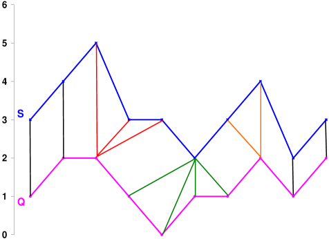
(a) The alignment of measurements for measuring the DTW distance between the two sequences $S$ and $Q$.

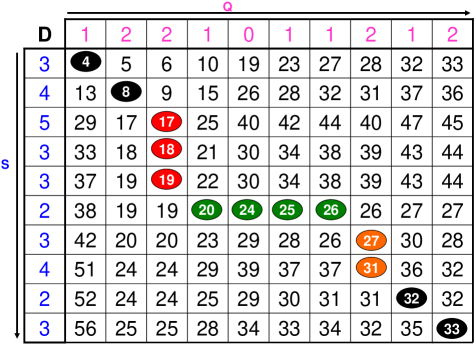
(b) The warping matrix $D$ produced by DTW; highlighted cells constitute the optimal warping path.

Figure 1: Illustration of DTW.

Algorithm 1 DTW: The standard DTW algorithm.

0:  $S$: Sequence of length $n$, $Q$: Sequence of length $m$.

0:  DTW distance.

1:  Initialize $D(i,1)\Leftarrow i\delta$ for each i

2:  Initialize $D(1,j)\Leftarrow j\delta$ for each j

3:  for all $i$ such that $2\leq i\leq n$ do

4:     for all $j$ such that $2\leq j\leq m$ do

5:        Use Equation 3 to compute $D(i,j)$

6:     end for

7:  end for

8:  return  $D(n,m)$

3 Dynamic Time Warping (DTW)

DTW is a dynamic programming technique used for measuring the similarity between any two time series with arbitrary lengths. This section gives an overview of DTW and how it is calculated. The following two time series (Equations 1 and 2) will be used in our explanations.

$$S = s_{1},s_{2},s_{3},\cdots,s_{i},\cdots,s_{n}$$ (1)

$$Q = q_{1},q_{2},q_{3},\cdots,q_{j},\cdots,q_{m}$$ (2)

Where $n$ and $m$ represent the length of time series $S$ and $Q$, respectively. $i$ and $j$ are the point indices in the time series.

DTW is a time series association algorithm that was originally used in speech recognition (Sakoe & Chiba, 1978). It relates two time series of feature vectors by warping the time axis of one series onto another.

As a dynamic programming technique, it divides the problem into several sub-problems, each of which contribute in calculating the distance cumulatively. Equation 3 shows the recursion that governs the computations is:

$$D(i,j)=d(i,j)+min\left\{\begin{array}[]{l}D(i-1,j)\\ D(i-1,j-1)\\ D(i,j-1).\end{array}\right.$$ (3)

The first stage in the DTW algorithm is to fill a local distance matrix $d$. That matrix has $n\times m$ elements which represent the Euclidean distance between every two points in the time series (i.e., distance matrix). In the second stage, it fills the warping matrix $D$ (Figure 1(b)) on the basis of Equation 3. Lines 1 to 7 in Algorithm 1 illustrate the process of filling the warping matrix. We refer to the cost between the $i^{th}$ and the $j^{th}$ elements as $\delta$ as mentioned in line 1 and 2.

After filling the warping matrix, the final stage for the DTW is to report the optimal warping path and the DTW distance. Warping path is a set of adjacent matrix elements that identify the mapping between $S$ and $Q$. It represents the path that minimizes the overall distance between $S$ and $Q$. The total number of elements in the warping path is $K$, where $K$ denotes the normalizing factor and it has the following attributes:

$$W=w_{1},w_{2},\ldots,w_{K}$$

$$max(|S|,|Q|)\leq K<(|S|+|Q|)$$

Every warping path must satisfy the following constraints (Keogh & Ratanamahatana, 2004; Salvador & Chan, 2007; Sakoe & Chiba, 1978):

1. Monotonicity: Any two adjacent elements of the warping path $W$, $w_{k}=(w_{i},w_{j})$ and $w_{k-1}=(w_{i}^{{}^{\prime}},w_{j}^{{}^{\prime}})$, follow the inequalities, $w_{i}-w_{i}^{{}^{\prime}}\geq 0$ and $w_{j}-w_{j}^{{}^{\prime}}\geq 0$. This constrain guarantees that the warping path will not roll back on itself. That is, both indexes $i$ and $j$ either stay the same or increase (they never decrease).

2. Continuity: Any two adjacent elements of the warping path $W$,$w_{k}=(w_{i},w_{j})$ and $w_{k+1}=(w_{i}^{{}^{\prime}},w_{j}^{{}^{\prime}})$, follow the inequalities, $w_{i}-w_{i}^{{}^{\prime}}\leq 1$ and $w_{j}-w_{j}^{{}^{\prime}}\leq 1$. This constraint guarantees that the warping path advances one step at a time. That is, both indexes $i$ and $j$ can only increase by at most 1 on each step along the path.

3. Boundary: The warping path starts from the top left corner $w_{1}=(1,1)$ and ends at the bottom right corner $w_{k}=(n,m)$. This constraint guarantees that the warping path contains all points of both time series.

Although there are a large number of warping paths that satisfy all of the above constraints, DTW is designed to find the one that minimizes the warping cost (distance). Figures 1(a) and 1(b) demonstrate an example of how two time series ($S$ and $Q$) are warped and the way their distance is calculated. The circled cells show the optimal warping path, which crosses the grid from the top left corner to the bottom right corner. The DTW distance between the two time series is calculated based on this optimal warping path using the following equation:

$$DTW(S,Q)=min\left\{\frac{\sqrt{\sum_{k=1}^{K}W_{k}}}{K}\right.$$ (4)

The $K$ in the denominator is used to normalize different warping paths with different lengths.

Since the DTW has to potentially examine every cell in the warping matrix, its space and time complexity is $O(nm)$.

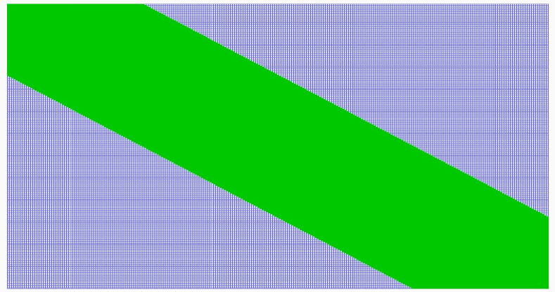
Figure 2: Global constraint (Sakoe Chiba Band), which limits the warping scope. The diagonal green areas correspond to the warping scopes.

4 Global Constraint (BandDTW)

There are several methods that add global constraints on DTW to increase its speed by limiting how far the warping path may stray from the diagonal of the warping matrix (Tappert & Das, 1978; Berndt & Clifford, 1994; Myers et al., 1980). In this paper we use Sakoe-Chiba Band (henceforth, we refer to it as BandDTW) Sakoe & Chiba (1978) when comparing with our proposed algorithm (Figure 2). BandDTW used to speed up the DTW by adding constraints which force the warping path to lie within a band around the diagonal; if the optimal path crosses the band, the DTW distance will not be optimal.

Algorithm 2 DC: Divide and Conquer technique.

0:  $S$: Sequence of length $n$, $Q$: Sequence of length $m$.

0:  DTW distance.

1:  Divide-Conquer-Alignment(S,Q)

2:  $n\Leftarrow|S|$

3:  $m\Leftarrow|Q|$

4:  $Mid\Leftarrow\lceil m/2\rceil$

5:  if $n\leq 2$ or $m\leq 2$ then

6:     Compute optimal alignment using standard DTW

7:  else

8:     $f\Leftarrow$ ForwardsSpaceEfficientAlign(S,Q[1:Mid])

9:     $g\Leftarrow$BackwardsSpaceEfficientAlign(S,Q[Mid:m])

10:     $q\Leftarrow$ index that minimizing $f(q,Mid)+g(q,Mid)$

11:     Add (q,Mid) to global array P

12:     Divide-Conquer-Alignment(S[1:q],Q[1:Mid])

13:     Divide-Conquer-Alignment(S[q:n],Q[Mid:m])

14:  end if

15:  return  P

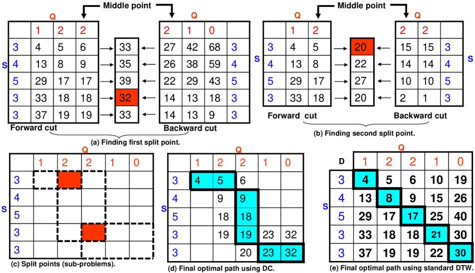
Figure 3: An example to show the difference between the standard DTW and the DC algorithm.

5 Divide and Conquer Technique (DC)

In the previous section, we have shown how to compute the optimal alignment using the standard DTW technique between two time series. In this section we will show another technique that uses a Divide and Conquer heuristic, henceforth we refer to it as (DC), proposed by Hirschberg (1975). DC is a dynamic programming algorithm used to find the least cost sequence alignment between two strings. The algorithm was first introduced to solve the Longest Common Subsequence (LCSS) (Hirschberg, 1975). Algorithm 2 gives a high level description of the DC algorithm. Like in the standard sequence alignment, the DC algorithm has $O(mn)$ time complexity but $O(m+n)$ space complexity, where $m$ and $n$ are the lengths of the two sequences being aligned. We will be using Algorithm 2 along with Figure 3 to explain how DC works. In the example we use two sequences $S=[3,4,5,3,3]$ and $Q=[1,2,2,1,0]$ to determine the optimal alignment between them. There is only one optimal alignment for this example (Figure 3(e)), where shaded cells are the optimal warping path. The DC algorithm works as follows:

1. It finds the middle point in $Q$ which is $Mid=|Q|/2$, (Figure 3(a)). This helps to find the split point which divides the warping matrix into two parts (sub-problems). A forward space efficiency function (Line 8) uses $S$ and the first cut of $Q=[1,2,2]$, then a backward step (Line 9) uses $S$ and $Q=[2,1,0]$ (Figure 3(a)). Then by adding the last column from the forward and backward steps together and finding the index of the minimum value, the resultant column indicates the row index that will be used along with the middle point to locate the split point (shaded cell in Figure 3(a)). Thus, the first split point is D(4,3). At this stage of the algorithm, there are two sub-problems; the alignment of $S=[3,4,5,3]$ with $Q=[1,2,2]$ and of $S=[3,3]$ with $Q=[2,1,0]$.

2. DC is recursive algorithm, each call splits the problem into two other sub-problems if both sequences are of $length>2$, otherwise it calls the standard DTW to find the optimal path for that particular sub-problem. In the example, the first sub-problem will be fed to Line 12 which will find another split point, because both input sequences are of length $>2$. Figure 3(b) shows how the new split point is found. Figure 3(c) shows the two split points (shaded cells) which yield to have sub-problems of sequences of length $\leq 2$. In this case DTW will be used to find the optimal alignment for each sub-problem.

3. The DC algorithm finds the final alignment by concatenating the results from each call of the standard DTW.

The example in Figure 3 clarifies that the DC algorithm does not give the optimal warping path. Figures 3(d) and (e) show the paths obtained by the DC and DTW algorithms, respectively.

DC does not yield the optimal path as it goes into infinite recursion because of how it calculates the middle point. DC calculates the middle point as follows:

There are two scenarios: first, when the middle point (Algorithm 2 Line 4) is floored ($Mid=\lfloor m/2\rfloor$) and second when it is rounded up ($Mid=\lceil m/2\rceil$). The first scenario causes infinite recursion, since the split from the previous step gives the same sub-sequences (i.e., the algorithm keeps finding the same split point). The second scenario is shown in Figures 3(a-d), which clearly confirms that the final optimal path is not the same as the one retrieved by the standard DTW . The final DTW distance is different as well. The shaded cells in Figures 3(d) and (e) show that both warping paths are different.

6 Sparse Dynamic Programming Approach

In this section, we outline the main principles we use in SparseDTW and follow up with an illustrated example along with the SparseDTW pseudo-code. We exploit the following facts in order to reduce space usage while avoiding any re-computations:

1. Quantizing the input time series to exploit the similarity between the points in the two time series.

2. Using a sparse matrix of size $k$, where $k=n\times m$ in the worst case. However, if the two sequences are similar, $k$ $<<n\times m$.

3. The warping matrix is calculated using dynamic programming and sparse matrix indexing.

6.1 Key Concepts

In this section we introduce the key concepts used in our algorithm.

Definition 1 (Sparse Matrix $SM$)

is a matrix that is populated largely with zeros. It allows the techniques to take advantage of the large number of zero elements. Figure 4(a) shows the $SM$ initial state. $SM$ is linearly indexed, The little numbers, in the top left corner of $SM$’s cells, represent the cell index. For example, the indices of the cells $SM(1,1)$ and $SM(5,5)$ are 1 and 25, respectively.

Definition 2 (Lower Neighbors ($LowerNeighbors$))

a cell $c\in SM$ has three lower neighbors which are the cells of the indices ($c-1$), ($c-n$), and ($c-(n+1)$) (where $n$ is the number of rows in $SM$) . For example, the lower neighbors of cell $SM(12)$ are $SM(6)$, $SM(7)$ and $SM(11)$ (Figure 4(a)).

Definition 3 (Upper Neighbors ($UpperNeighbors$))

a cell $c\in SM$ has three upper neighbors which are the cells of the indices ($c+1$), ($c+n$), and ($c+n+1$) (where $n$ is the number of rows in $SM$) . For example, the upper neighbors of cell $SM(12)$ are $SM(13)$, $SM(17)$ and $SM(18)$ (Figure 4(a)).

Definition 4 (Blocked Cell (B))

a cell $c\in SM$ is blocked if its value is zero. The letter (B) refers to the blocked cells (Figure 4(a)).

Definition 5 (Unblocking)

Given a cell $c\in SM$, if $SM(c)$’s upper neighbors ($SM(c+1)$,$SM(c+n)$, and $SM(c+n+1)$) are blocked, they will be unblocked. Unblocking is performed by calculating the EucDist for these cells and adding them to $SM$. In other words, adding the distances to these cells means changing their state from blocked (B) into unblocked. For example, $SM(10)$ is a blocked upper neighbor of $SM(5)$, in this case $SM(10)$ needs to be unblocked (Figure 4(c)).

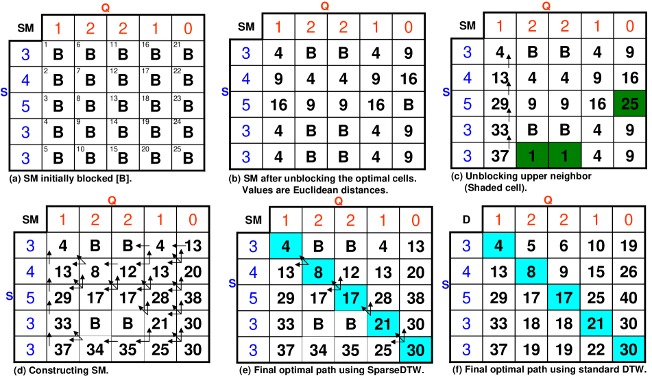
Figure 4: An example of the SparseDTW algorithm and the method of finding the optimal path.

6.2 SparseDTW Algorithm

Algorithm 3 takes $Res$, the resolution parameter as an input that determines the number of bins as $\frac{2}{Res}$. $Res$ will have no impact on the optimality. We now present an example of our algorithm to illustrate some of the highlights of our approach: We start with two sequences:

$S=[3,4,5,3,3]$ and $Q=[1,2,2,1,0]$.

In Line 1, we first quantize the sequences into the range $[0,1]$ using Equation 5:

$$QuantizedSeq_{i}^{k}=\frac{S_{i}^{k}-min(S^{k})}{max(S^{k})-min(S^{k})}.$$ (5)

Where $S_{i}^{k}$ denotes the $i^{th}$ element of the $k^{th}$ time series. This yields the following sequences:

$S^{\prime}=[0,0.5,1.0,0.0,0.0]$ and $Q^{\prime}=[0.5,1.0,1.0,0.5,0]$

In Lines 4 to 7 we create overlapping bins, governed by two parameters: bin-width and the overlapping width (which we refer to as the resolution). It is important to note that these two parameters do not affect the optimality of the alignment but do have an affect on the amount of space utilized. For this particular example, the bin-width is 0.5. We thus have 4 bins which are shown in Table 1.

Bin Number	Bin	Indices	Indices
($B_{k}$)	Bounds	of $S^{\prime}$	of $Q^{\prime}$
1	0.0-0.5	1,2,4,5	1,4,5
2	0.25-0.75	2	1,4
3	0.5-1.0	2,3	1,2,3,4
4	0.75-1.25	3	2,3

Table 1: Bins bounds, where $B_{k}$ is the $k^{th}$ bin.

Our intuition is that points in sequences with similar profiles will be mapped to other points in the same bin or neighboring bins. In which case the non-default entries of the sparse matrix can be used to compute the warping path. Otherwise, default entries of the matrix will have to be “opened”, reducing the sparsity of the matrix but never sacrificing the optimal alignment.

In Lines 3 to 13, the sparse warping matrix $SM$ is constructed using the equation below. $SM$ is a matrix that has generally few non-zero (or “interesting”) entries. It can be represented in much less than $n\times m$ space, where $n$ and $m$ are the lengths of the time series $S$ and $Q$, respectively.

$$\centering SM(i,j)=\left\{\begin{array}[]{ll}EucDist(S(i),Q(j))&\mbox{\small{if $S(i)$ and $Q(j)\in B_{k}$}}\\ B&otherwise\end{array}\right.\@add@centering$$ (6)

We assume that $SM$ is linearly ordered and the default value of $SM$ cells are zeros. That means the cells initially are Blocked (B) (Figure 4(a)). Figure 4(a) shows the linear order of the $SM$ matrix, where the little numbers on the top left corner of each cell represent the index of the cells. In Line 6 and 7, we find the index of each quantized value that falls in the bin bounds (Table 1 column 2, 3 and 4). The Inequality 7 is used in Line 6 and 7 to find the indices of the default entries of the $SM$.

$$LowerBound\leq QuantizedSeq^{k}_{i}\leq UpperBound.$$ (7)

Where $LowerBound$ and $UpperBound$ are the bin bounds and $QuantizedSeq^{k}_{i}$ represents the quantized time series which can be calculated using Equation 5.

Lines 8 to 12 are used to initialize the $SM$. That is by joining all indices in $idxS$ and $idxQ$ to open corresponding cells in $SM$. After unblocking (opening) the cells that reflect the similarity between points in both sequences, the $SM$ entries are shown in Figure 4(b).

Lines 14 to 22 are used to calculate the warping cost. In Line 15, we find the warping cost for each open cell $c\in SM$ (cell $c$ is the number from the linear order of $SM$’s cells) by finding the minimum of the costs of its lower neighbors, which are $[c-1,c-n,c-(n+1)]$ (black arrows in Figure 4(d) show the lower neighbors of every open cell). This cost is then added to the local distance of cell $c$ (Line 17). The above step is similar to DTW, however, we may have to open new cells if the upper neighbors at a given local cell $c\in SM$ are blocked. The indices of the upper neighbors are $[c+1,c+n,c+n+1]$ , where $n$ is the length of sequence $S$ (i.e., number of rows in $SM$). Lines 18 to 21 are used to check always the upper neighbors of $c\in SM$. This is performed as follows: if the $|UpperNeighbors|=0$ for a particular cell, its upper neighbors will be unblocked. This is very useful when the algorithm traverses $SM$ in reverse to find the final optimal path. In other words, unblocking allows the path to be connected. For example, the cell $SM(5)$ has one upper neighbor that is cell $SM(10)$ which is blocked (Figure 4(b)), therefore this cell will be unblocked by calculating the EucDist(S(5),Q(2)). The value will be add to the $SM$ which means that cell $SM(10)$ is now an entry in $SM$ (Figure 4(c)). Although unblocking adds cells to $SM$ which means the number of open cells will increase, but the overlapping in the bins boundaries allows the $SM$’s unblocked cells to be connected mostly that means less number of unblocking operations. Figure 4(d) shows the final entries of the $SM$ after calculating the warping cost of all open cells.

Lines 23 to 32 return the warping path. $hop$ initially represents the linear index for the $(m,n)$ entry of $SM$, that is the bottom right corner of $SM$ in Figure 4(e). Starting from $hop=n\times m$ we choose the neighbors [$hop-n,hop-1,hop-(n+1)$] with minimum warping cost and proceed recursively until we reach the first entry of $SM$, namely $SM(1)$ or $hop=1$. It is interesting that while calculating the warping path we only have to look at the open cells, which may be fewer in number than 3. This potentially reduces the overall time complexity.

Figure 4(e) demonstrates an example of how the two time series ($S$ and $Q$) are warped and the way their distance is calculated using SparseDTW. The filled cells show the optimal warping path, which crosses the grid from the top left corner to the bottom right corner. The distance between the two time series is calculated using Equation 4. Figure 4(f) shows the standard DTW where the filled cells are the optimal warping path. It is clear that both techniques give the optimal warping path which will yield the optimal distance.

Algorithm 3 SparseDTW: Sparse dynamic programming technique.

0:  $S$: Time series of length $n$, $Q$: Time series of length $m$, and Res.

0:  Optimal warping path and SparseDTW distance.

1:  $[S^{\prime},Q^{\prime}]\Leftarrow Quantize(S,Q)$

2:  $LowerBound\Leftarrow 0$, $UpperBound\Leftarrow Res$

3:  for all $0\leq LowerBound\leq 1-\frac{Res}{2}$ do

4:     $IdxS\Leftarrow find(LowerBound\leq S^{\prime}\leq UpperBound)$

5:     $IdxQ\Leftarrow find(LowerBound\leq Q^{\prime}\leq UpperBound)$

6:     $LowerBound\Leftarrow LowerBound+\frac{Res}{2}$

7:     $UpperBound\Leftarrow LowerBound+Res$

8:     for all $idx_{i}\in IdxS$ do

9:        for all $idx_{j}\in IdxQ$ do

10:           Add $EucDist(idx_{i},idx_{j})$ to $SM$ {When $EucDist(idx_{i},idx_{j})=0,SM(i,j)=-1$.}

11:        end for

12:     end for

13:  end for{Note: $SM$ is linearly indexed.}

14:  for all $c\in SM$ do

15:     $LowerNeighbors\Leftarrow\{(c-1),(c-n),(c-(n+1))\}$

16:     $minCost\Leftarrow min(SM(LowerNeighbors))$ {SM(LowerNeighbors)=-1 means cost=0.}

17:     $SM(c)\Leftarrow SM(c)+minCost$

18:     $UpperNeighbors\Leftarrow\{(c+1),(c+n),(c+n+1)\}$

19:     if $|UpperNeighbors|==0$ then

20:        $SM\cup EucDist(UpperNeighbors)$

21:     end if

22:  end for

23:  $WarpingPath\Leftarrow\Phi$

24:  $hop\Leftarrow SM(n\times m)$ {Last index in SM.}

25:  $WarpingPath\cup hop$

26:  while $hop\neq SM(1)$ do

27:     $LowerNeighbors\Leftarrow\{(hop-1),(hop-n),(hop-(n+1))\}$

28:     [minCost,index]$\Leftarrow$ min[Cost([LowerNeighbors])

29:     $hop\Leftarrow index$

30:     $WarpingPath\cup hop$

31:  end while

32:  $WarpingPath\cup SM(1)$

33:  return  $WarpingPath,SM(n\times m)$

6.3 SparseDTW Complexity

Given two time series $S$ and $Q$ of length $n$ and $m$, the space and time complexity of standard DTW is $O(nm)$. For SparseDTW we attain a reduction by a constant factor $b$, where $b$ is the number of bins. This is similar to the BandDTW approach where the reduction in space complexity is governed by the size of the band. However, SparseDTW always yields the optimal alignment. The time complexity of SparseDTW is $O(nm)$ in the worst case as we potentially have to access every cell in the matrix.

7 Experiments, Results and Analysis

In this section we report and analyze the experiments that we have conducted to compare SparseDTW with other methods. Our main objective is to evaluate the space-time tradeoff between SparseDTW, BandDTW and DTW. We evaluate the effect of correlation on the running time of SparseDTW. As we have noted before, both SparseDTW and DTW always yield the optimal alignment while BandDTW results can often lead to sub-optimal alignments, as the optimal warping path may lie outside the band. As we noted before DC may not yield the optimal result.

7.1 Experimental Setup

All experiments were carried out on a Windows XP operated PC with a Pentium(R) D (3.4 GHz) processor and 2 GB main memory. The data structures and algorithm were implemented in C++.

7.2 Datasets

We have used a combination of benchmark and synthetically generated datasets. The benchmark dataset is a subset from the UCR time series data mining archive (Keogh, 2006). We have also generated synthetic time series data to control and test the effect of correlation on the running time of SparseDTW. We briefly describe the characteristics of each dataset used.

• GunX: comes from the video surveillance application and captures the shape of a gun draw with the gun in hand or just using the finger. The shape is captured using 150 time steps and there are a total of 100 sequences (Keogh, 2006). We randomly selected two sequences and computed their similarity using the three methods.

• Trace: is a synthetic dataset generated to simulate instrumentation failures in a nuclear power plant (Roverso, 2000). The dataset consists of 200 time series each of length 273.

• Burst-Water: is formed by combining two different datasets from two different applications. The average length of the series is 2200 points (Keogh, 2006).

• Sun-Spot: is a large dataset that has been collected since 1818. We have used the daily sunspot numbers. More details about this dataset exists in (Vanderlinden, 2008). The 1st column of the data is the year, month and day, the 2nd column is year and fraction of year (in Julian year), and the 3rd column is the sunspot number. The length of the time series is 2898.

• ERP: is the Event Related Potentials that are calculated on human subjects. The dataset consists of twenty sequences of length 256 (Makeig et al., 1999).

• Synthetic: Synthetic datasets were generated to control the correlation between sequences. The length of each sequence is 500.

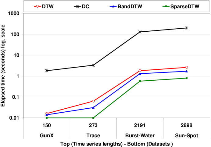
Figure 5: Elapsed time using real life datasets.

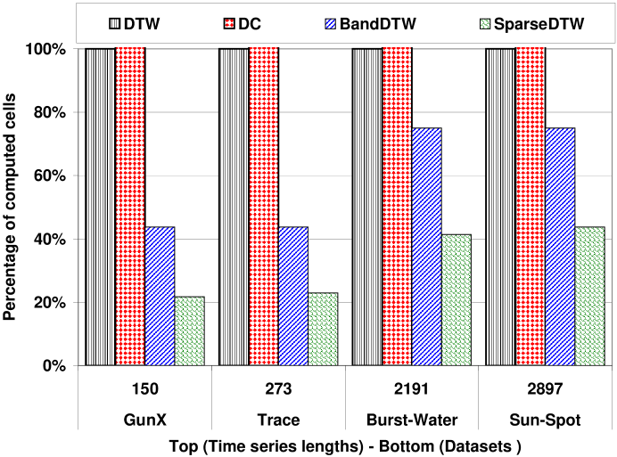
Figure 6: Percentage of computed cells as a measure for time complexity.

	Number of computed cells used by
Data
size	DTW	DC	BandDTW	SparseDTW
2K	$4\times 10^{6}$	$>8\times 10^{6}$	2500	2000
4K	$16\times 10^{6}$	$>30\times 10^{6}$	5000	4000
6K	$36\times 10^{6}$	$>70\times 10^{6}$	7500	6000

Table 2: Number of computed cells if the optimal path is close to the diagonal.

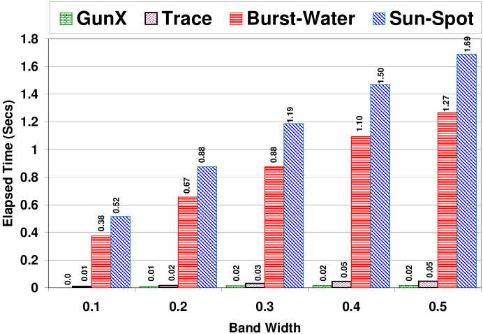
Figure 7: Effect of the band width on BandDTW elapsed time.

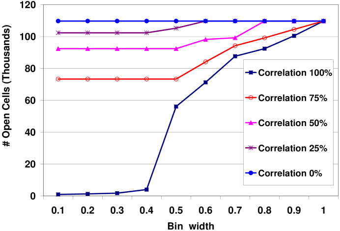
Figure 8: Effects of the resolution and correlation on SparseDTW.

Dataset	Algorithm	#opened	Elapsed
size	name	cells	Time(Sec.)
3K	DTW	$9\times 10^{6}$	7.3
	SparseDTW	614654	0.65
6K	DTW	$36\times 10^{6}$	26
	SparseDTW	2048323	2.2
9K	DTW	$81\times 10^{6}$	N.A
	SparseDTW	4343504	4.8
12K	DTW	$144\times 10^{6}$	N.A
	SparseDTW	7455538	200

Table 3: Performance of the DTW and SparseDTW algorithms using large datasets.

7.3 Discussion and Analysis

SparseDTW algorithm is evaluated against three other existing algorithms, DTW, which always gives the optimal answer, DC, and BandDTW.

Dataset	Algorithm	Number of	Warping path	Elapsed Time	DTW
name	name	opened cells	size (K)	(Seconds)	Distance
GunX	DTW	22500	201	0.016	0.01
	BandDTW	448	152	0.000	0.037
	SparseDTW	4804	201	0.000	0.01
Trace	DTW	75076	404	0.063	0.002
	BandDTW	1364	331	0.016	0.012
	SparseDTW	17220	404	0.000	0.002
Burst-Water	DTW	2190000	2190	1.578	0.102
	BandDTW	43576	2190	0.11	0.107
	SparseDTW	951150	2190	0.75	0.102
Sun-Spot	DTW	1266610	357	0.063	0.021
	BandDTW	12457	358	0.016	0.022
	SparseDTW	66049	357	0.016	0.021
ERP	DTW	1000000	1533	0.78	0.008
	BandDTW	19286	1397	0.047	0.013
	SparseDTW	210633	1535	0.18	0.008
Synthetic	DTW	250000	775	0.187	0.033
	BandDTW	4670	600	0.016	0.043
	SparseDTW	105701	775	0.094	0.033

Table 4: Statistics about the performance of DTW, BandDTW, and SparseDTW. Results in this table represent the average over all queries.

7.3.1 Elapsed Time

The running time of the four approaches is shown in Figure 5. The time profile of both DTW and BandDTW is similar and highlights the fact that BandDTW does not exploit the nature of the datasets. DC shows as well the worst performance due to the vast number of recursive calls to generate and solve sub-problems. In contrast, it appears that SparseDTW is exploiting the inherent similarity in the GunX and Trace data.

In Figure 6 we show the number of open/computed cells produced by the four algorithms. It is very clear that SparseDTW produces the lowest number of opened cells.

In Table 2 we show the number of computed cells that are used in finding the optimal alignment for three different datasets, where their optimal paths are close to the diagonal. DC has shown the highest number of computed cells followed by DTW. That is because both (DC and DTW) do not exploit the similarity in the data. BandDTW has shown interesting results here because the optimal alignment is close to the diagonal. However, SparseDTW still outperforms it.

Two conclusions are revealed from Figure 7. The first, the length of the time series affects the computing time, because the longer the time series the bigger the matrix. Second, band width influences CPU time when aligning pairs of time series. The wider the band the more cells are required to be opened.

DTW and SparseDTW are compared together using large datasets. Table 3 shows that DTW is not applicable (N.A) for datasets of size $>6K$, since it exceeds the size of the memory when computing the warping matrix. In this experiment we excluded BandDTW and DC given that they provide no guarantee on the optimality.

To determine the effect of correlation on the elapsed time for SparseDTW we created several synthetic datasets with different correlations. The intuition being that two sequences with lower correlation will have a warping path which is further away from the diagonal and thus will require more open cells in the warping matrix. The results in Figure 8 confirm our intuition though only in the sense that extremely low correlation sequences have a higher number of open cells than extremely high correlation sequences.

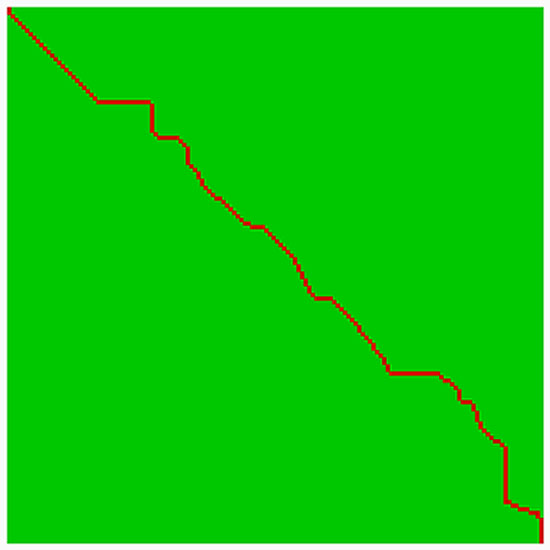
(a) GunX-DTW

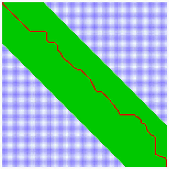
(b) GunX-BandDTW

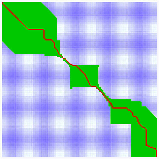
(c) GunX-SparseDTW

Figure 9: The optimal warping path for the GunX and Trace sequences using three algorithms (DTW, BandDTW, and SparseDTW). The advantages of SparseDTW are clearly revealed as only a small fraction of the matrix cells have to be “opened” compared to the other two approaches.

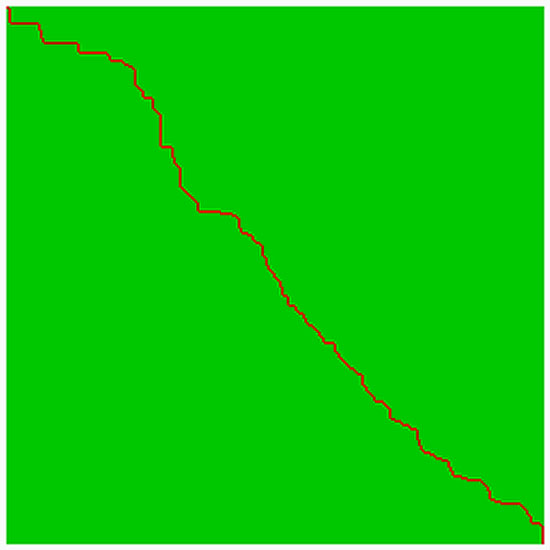
(d) Trace-DTW

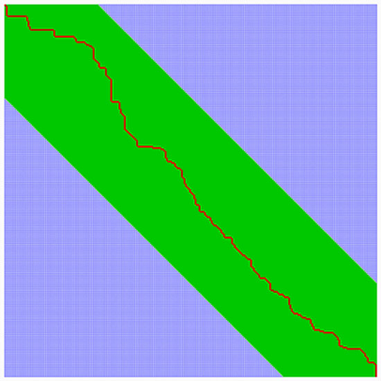
(e) Trace-BandDTW

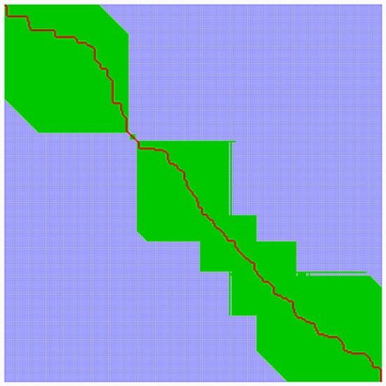
(f) Trace-SparseDTW

7.3.2 SparseDTW Accuracy

The accuracy of the warping path distance of BandDTW and SparseDTW compared to standard DTW (which always gives the optimal result) is shown in Table 4. It is clear that the error rate of BandDTW varies from 30% to 500% while SparseDTW always gives the exact value. It should be noticed that there may be more than one optimal path of different sizes but they should give the same minimum cost (distance). For example, the size of the warping path for the ERP dataset produced by DTW is 1533, however, SparseDTW finds another path of size 1535 with the same distance as DTW.

Figure 9(c) shows the dramatic nature in which SparseDTW exploits the similarity inherent in the sequences and creates an adaptive band around the warping path. For both the GunX and the Trace data, SparseDTW only opens a fraction of the cells compared to both standard DTW and BandDTW.

8 Conclusions

In this paper we have introduced the SparseDTW algorithm, which is a sparse dynamic programming technique. It exploits the correlation between any two time series to find the optimal warping path between them. The algorithm finds the optimal path efficiently and accurately. SparseDTW always outperforms the algorithms DTW, BandDTW and DC. We have shown the efficiency of the proposed algorithm through comprehensive experiments using synthetic and real life datasets.

References

- (1)
- Berndt & Clifford (1994) Berndt, D. J. & Clifford, J. (1994), Using dynamic time warping to find patterns in time series, in ‘Association for the Advancement of Artificial Intelligence, Workshop on Knowledge Discovery in Databases (AAAI)’, pp. 229–248.
- Caiani et al. (1998) Caiani, E., Porta, A., Baselli, G., Turie, M., Muzzupappa, S., Piemzzi, Crema, C., Malliani, A. & Cerutti, S. (1998), ‘Warped-average template technique to track on a cycle-by-cycle basis the cardiac filling phases on left ventricular volume’, Computers in Cardiology 5, 73–76.
- Capitani & Ciaccia (2007) Capitani, P. & Ciaccia, P. (2007), ‘Warping the time on data streams’, Data and Knowledge Engineering 62(3), 438–458.
- Hirschberg (1975) Hirschberg, D. (1975), ‘A linear space algorithm for computing maximal common subsequences’, Communications of the ACM 18(6), 341–343.
- Itakura (1975) Itakura, F. (1975), ‘Minimum prediction residual principle applied to speech recognition’, IEEE Transactions on Acoustics, Speech and Signal Processing 23(1), 67–72.
- Keogh (2006) Keogh, E. (2006), ‘The ucr time series data mining archive’, http://www.cs.ucr.edu/ eamonn/TSDMA/index.html.
- Keogh & Pazzani (2000) Keogh, E. & Pazzani, M. (2000), Scaling up dynamic time warping for datamining applications, in ‘Proceedings of the sixth ACM SIGKDD international conference on Knowledge discovery and data mining (KDD)’, ACM Press, New York, NY, USA, pp. 285–289.