Effective renormalized multi-body interactions of harmonically confined ultracold neutral bosons

Abstract

We calculate the renormalized effective two-, three-, and four-body interactions for $N$ neutral ultracold bosons in the ground state of an isotropic harmonic trap, assuming two-body interactions modeled with the combination of a zero-range and energy-dependent pseudopotential. We work to third-order in the scattering length $a_{\text{t}}(0)$ defined at zero collision energy, which is necessary to obtain both the leading-order effective four-body interaction and consistently include finite-range corrections for realistic two-body interactions. The leading-order, effective three- and four-body interaction energies are $U_{3}\left(\omega\right)=-(0.85576...)[a_{\text{t}}(0)/\sigma(\omega)]^{2}+2.7921(1)[a_{\text{t}}(0)/\sigma(\omega)]^{3}+\mathcal{O}(a_{\text{t}}^{4})$ and $U_{4}(\omega)=+(2.43317...)[a_{\text{t}}(0)/\sigma(\omega)]^{3}+\mathcal{O}(a_{\text{t}}^{4})$, where $\omega$ and $\sigma(\omega)$ are the harmonic oscillator frequency and length, respectively, and energies are in units of $\hbar\omega$. The one-standard deviation error $\pm 0.0001$ for the third-order coefficient in $U_{3}(\omega)$ is due to numerical uncertainty in estimating a slowly converging sum; the other two coefficients are either analytically or numerically exact. The effective three- and four-body interactions can play an important role in the dynamics of tightly confined and strongly correlated systems. We also performed numerical simulations for a finite-range boson–boson potential, and it was comparison to the zero-range predictions which revealed that finite-range effects must be taken into account for a realistic third-order treatment. In particular, we show that the energy-dependent pseudopotential accurately captures, through third order, the finite-range physics, and in combination with the multi-body effective interactions gives excellent agreement with the numerical simulations, validating our theoretical analysis and predictions.

I Introduction

Effective multi-body interactions arise when quantum fluctuations dress the intrinsic interactions between particles. They play a central role in quantum field theories and exemplify the significant difference between interactions in classical and quantum theories. For example, even for a quantum field that has only intrinsic two-body interactions at high energies, at low-energy scales, after the high-energy degrees of freedom are coarse-grained away, the field will manifest at some level effective $n$-body interactions. The ability to trap and control systems of ultracold neutral atoms Bloch et al. (2008); Chin et al. (2010) has created new opportunities to study this physics in the laboratory. Effective three-body interactions in the limit of large two-body scattering length have in particular received a great deal of attention, motivated both by the predictions of universal behaviors Efimov (1970); Nielsen and Macek (1999); Esry et al. (1999); Bedaque et al. (2000); Kraemer et al. (2006); Braaten and Hammer (2007, 2006) and the ability to use ultracold atoms to study physics ranging from molecular Torrontegui et al. (2011) to nuclear scales Beane et al. (2007); Maeda et al. (2009). Recently, attention has focused on Efimov-like states and universal behaviors for four-body systems, again in the limit of large scattering lengths Hammer and Platter (2007); von Stecher et al. (2009); Pollack et al. (2009); Ferlaino et al. (2009).

Here, we focus on the opposite regime of weakly interacting neutral bosons with small scattering lengths. Even in this limit, effective higher-body interactions can be important, particularly for tightly confined or strongly correlated particles. This is seen dramatically in Will et al. (2010), where a superfluid of bosonic atoms is quenched by suddenly increasing the depth of an optical lattice. After the quench, which creates a non-equilibrium state of strongly correlated bosons, beating effects due to multiple distinct interaction energies, as expected from effective three- and higher-body interactions Johnson et al. (2009); Tiesinga and Johnson (2011), are seen in the collapse and revival oscillations of the first-order coherence. Effective multi-body interactions should also have played a role in previous collapse and revival experiments Greiner et al. (2002); Anderlini et al. (2006); Sebby-Strabley et al. (2007), although in those cases inhomogeneities may have masked their signature. More recently, effective three- and four-body interactions have been used to demonstrate atom-number sensitive photon-assisted tunneling in optical lattices Ma et al. (2011), and their influence has been seen in precision measurements on Mott-insulator states of ultracold atoms Mark et al. (2011). A number of studies also suggest that elastic multi-body interactions can play an interesting role in generating exotic quantum phases in optical lattices or modifying the superfluid to Mott-insulator phase transition Büchler et al. (2007); Chen et al. (2008); Schmidt et al. (2008); Capogrosso-Sansone et al. (2009); Mazza et al. (2010); Zhou et al. (2010); Will et al. (2011); Singh et al. (2012).

In this paper, we use renormalized quantum field theory Srednicki (2007) to calculate the perturbative ground-state energy for $N$ ultracold neutral bosons in a three dimensional isotropic harmonic potential with angular frequency $\omega,$ and extract from it the effective $m$-body interaction energies $U_{2}(\omega),$ $U_{3}(\omega),$ and $U_{4}(\omega)$ as a function of $\omega.$ The key purpose of the present paper is to (i) systematically develop a renormalized quantum field theory approach for ultracold trapped bosons including finite-range effects, (ii) determine the leading-order four-body interaction, and (iii) validate the formalism through comparison with numerical results. To obtain effective four-body interaction energies it is necessary to work through third order in the two-body scattering length. We use renormalized perturbation theory (see Srednicki (2007)), which develops an expansion around physical as opposed to bare coupling parameters, to systematically cancel the multiple divergences that arise at higher-orders in quantum field perturbation theory. (In this paper, the physical coupling parameter is defined in terms of the measured scattering length, or alternatively the measured energy shift, for two interacting ultracold boson in a harmonic trap at a specified trap frequency.) Renormalized perturbation theory, which is more commonly used in high-energy physics, in this context naturally describes how the effective interactions depend on trap frequency. An example of the power of renormalized perturbation theory to capture low-energy physics is that we independently reproduce, through third order, the two-body ground-state energies calculated in Busch et al. (1998). More fundamentally, the analysis in this paper provides an explicit example of renormalization physics and running coupling constants that can be directly probed using trapped ultracold bosonic atoms, and used to test central concepts in effective field theory.

To calculate effective interactions for confined bosons, we first assumed that the two-body interactions could be described in the low-energy, $s$-wave limit by an energy-independent zero-range $\delta$-function pseudopotential. To test our perturbative predictions, we then numerically calculated $N$-boson ground-state energies using a finite-range two-body Gaussian model potential. Comparison with the numerical results revealed that finite-range effects must also be taken into account for an accurate description of realistically interacting bosons. In this paper, we show that both the finite range effects and effective interactions are accurately captured by the combination of zero-range and energy-dependent $\delta$-function pseudopotentials. Including the finite-range corrections, we are able to validate our analytic and numerical calculations of all perturbation theory coefficients through third order.

The basic idea in our approach is the following: we “integrate out” excited vibrational states thereby trading a multi-orbital theory with intrinsic two-body interactions for a single-orbital theory with effective multi-body interactions. The latter can provide a simple but powerful alternative description of the low-energy few-body physics. The quantum fluctuations to excited states both dress the two-body interactions and generate effective higher-body interactions. The idea is illustrated in Fig. 1. We showed in Johnson et al. (2009); Tiesinga and Johnson (2011) how this approach can be used to approximately incorporate the influence of higher bands via the simple modification of adding higher-body interactions to the single-band Bose-Hubbard model Fisher et al. (1989); Jaksch et al. (1998).

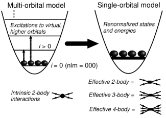
Figure 1: Illustration of the idea of replacing a multiple-orbital (or multiple-band) model with orbitals $i=0,1,...$ with only intrinsic two-body interactions by a single-orbital (or single-band) model with effective multi-body interactions between renormalized states. A ground state multi-body model can be useful when virtual excitations of bosons to excited vibrational levels are important.

Beyond applying directly to ultracold neutral bosons in an isotropic harmonic potential, our results can give qualitative insight into the effective interactions for other trapping potentials. They can also be used for rough approximations to the effective two-, three-, and four-body interactions in anisotropic potentials, and for neutral bosons in optical lattices. In the latter case, however, anharmonicities are important. For example, we estimate an approximately 30% anharmonic correction to the three-body interactions for ⁸⁷Rb in typical lattices. The role of anharmonicities for collapse-and-revival dynamics in optical lattice systems has been analyzed further in Mering and Fleischhauer (2011). Inhomogeneities and the effect of a background harmonic potential on lattice collapse-and-revival dynamics has been studied in Schachenmayer et al. (2011); Buchhold et al. (2011).

Tunneling also has an influence on collapse and revival in optical lattices Rigol et al. (2006); Fischer and Schützhold (2008); Wolf et al. (2010). In deep (post-quench) lattices the typical tunneling energy is nearly an order of magnitude smaller than the effective three-body interaction energy, making the latter effect dominant. Tunneling should, however, be of comparable importance to the effective four-body interactions. Approaches applying effective interaction methods to tunneling in lattice or multi-well systems include Ananikian and Bergeman (2006); Fölling et al. (2007); Zhou et al. (2011); Pielawa et al. (2011), and related methods for analyzing physics involving interactions, correlations, higher bands, and quantum tunneling in lattice systems include Alon et al. (2005, 2007); Hazzard and Mueller (2010); Lühmann et al. (2012); Bissbort et al. (2011); Cao et al. (2011). Fermionic systems and fermion-boson mixtures also yield interesting types of effective interactions that have received increasing attention (e.g., Blume et al. (2007); Lühmann et al. (2008); Lutchyn et al. (2009); Mering and Fleischhauer (2011); Rotureau et al. (2010); Will et al. (2011)), as well as three-body interactions of fermions and polar molecules in lattices Büchler et al. (2007).

For experiments with ⁸⁷Rb at typical lattice densities the recombination rate Burt et al. (1997); Esry et al. (1999) is one or more orders of magnitude smaller than the frequencies associated with both the effective three- and four-body energies, and therefore the elastic effective interactions described in the present paper are more important than inelastic multi-body interactions driving loss. Roughly, we expect three-body recombination to scale at fourth order in the scattering length Fedichev et al. (1996), and in the future we would like to understand both elastic and inelastic interactions in a unified framework. The role of effective three-body interactions in thermalizing a homogenous 1D Bose gas has also been studied Mazets and Schmiedmayer (2010), and it would be interesting to investigate this physics in the context of a 3D optical lattice system.

The remainder of this paper is organized as follows. In Sec. II, we provide an overview of our results. Section III compares the perturbation theory predictions to numerical estimates for finite-range interactions. Sections IV and V describe the details of the renormalized perturbation theory used to obtain the effective multi-body interactions. Section IV defines the renormalized Hamiltonian and derives the first- and second-order corrections, while Sec. V derives the two-, three-, and four-body interaction energies through third order. Section VI summarizes our results and conclusions. Finally, the appendices give derivations of a number of technical results used in the paper.

II Overview

We find the effective interactions of $N$ ultracold bosons in the ground state of an isotropic harmonic oscillator with pairwise interactions modeled by a zero-range $\delta$-function pseudopotential

$$\mathcal{V}_{2}(\mathbf{r}_{i}-\mathbf{r}_{j})=g_{2}\delta^{(3)}(\mathbf{r}_{i}-\mathbf{r}_{j}),$$ (1)

where $\mathbf{r}_{i}$ is the position vector of the $i^{\text{th}}$ boson. We assume there are no intrinsic three- or higher-body interactions. The two-body coupling constant $g_{2}$ is related to $a_{\text{t}}(0)$, at first order in perturbation theory, by $g_{2}=4\pi\left(\hbar^{2}/m_{\text{A}}\right)a_{\text{t}}(0)+\mathcal{O}([a_{\text{t}}(0)]^{2}),$ where $m_{\text{A}}$ is the boson mass, $a_{\text{t}}(0)$ is the physical $s$-wave scattering length measured in the limit that the trap frequency and collision energy go to zero, and $\mathcal{O}([a_{\text{t}}(0)]^{2})$ are terms of order $[a_{\text{t}}(0)]^{2}$ and higher. At higher orders, the relationship between $g_{2}$ and $a_{\text{t}}(0)$ is modified, and in Secs. IV and V we generalize the perturbation theory as an expansion around the physical trap scattering length $a_{\text{t}}(\omega_{0})$ defined for a harmonic potential with frequency $\omega_{0}.$ In this overview, we summarize our results to third order in $a_{\text{t}}(0),$ i.e., the special case $\omega_{0}=0.$

We obtain the ground-state energy of $N$ bosons as an expansion $E=\sum_{n=0}E^{(n)},$ where $E^{(n)}$ is proportional to $[a_{\text{t}}(0)]^{n}.$ Throughout this paper energies are expressed in units of the harmonic oscillator energy $\hbar\omega.$ The zeroth-order (one-body) energy is $E^{(0)}(\omega)=\varepsilon_{0}N,$ where $\varepsilon_{0}=3/2$ is the dimensionless single-particle ground-state energy. The $n^{\text{th}}$-order energies for $n>0$ can be expanded as

$$E^{(n)}=\sum_{m=2}\binom{N}{m}U_{m}^{(n)}(\omega),$$ (2)

where $\binom{N}{m}$ is the binomial coefficient. The sum goes up to the minimum of $N$ and $n+1$, and the $n^{\text{th}}$-order contributions to the $m$-body interaction energies (in units of $\hbar\omega)$ are

$$U_{m}^{(n)}(\omega)=c_{m}^{(n)}\left(\frac{a_{\text{t}}(0)}{\sigma(\omega)}\right)^{n},$$ (3)

where the harmonic oscillator length for an isotropic potential with frequency $\omega$ is

$$\sigma(\omega)=\sqrt{\hbar/m_{\text{A}}\omega}.$$ (4)

Table 1 gives the values of $c_{m}^{(n)}$ obtained in Secs. IV and V. The two-body coefficients $c_{2}^{(1)},c_{2}^{(2)},$ and $c_{2}^{(3)}$ independently reproduce the results in Busch et al. (1998), if the exact solution found there is expanded through third order. The coefficient $c_{2}^{(3)}$, in particular, is nontrivial and provides a strong consistency check that the renormalized perturbation theory captures the two-body low-energy interactions correctly.

The analytic value of the three-body coefficient $c_{3}^{(2)}$ was previously found in Johnson et al. (2009). The coefficient $c_{3}^{(3)}$ found here extends that result to third order in $a_{\text{t}}(0)$. The value of $c_{3}^{(3)}$ given in Table 1 combines both analytic and approximate numerical results, and the uncertainty is due to the slow convergence of one of the numerically determined sums (see App. B.2).

We also obtain the coefficient $c_{4}^{(3)},$ which gives the leading-order contribution to the effective four-body energy. The coefficient $c_{4}^{(3)}$ combines numerical and analytic results, but unlike $c_{3}^{(3)}$ has high precision because of the fast convergence of all the contributing terms. Note that $c_{3}^{(3)}$ and $c_{4}^{(3)}$ have similar magnitudes, and consequently we need to include the effective three-body corrections when effective four-body effects are important or of interest. At the end of Sec. II, we show that the correction from the third-order terms becomes significant for ultracold atoms in trap potentials with relatively tight confinement. The coefficients $c_{3}^{(3)}$ and $c_{4}^{(3)}$ have not previously been reported in the literature.

Effective Interaction Energy Coefficients       Two-body $c_{2}^{(1)}=(2/\pi)^{1/2}=+0.79788...$ $c_{2}^{(2)}=(2/\pi)(1-\log 2)=+0.19535...$ $c_{2}^{(3)}=(2/\pi)^{3/2}(1-\frac{\pi^{2}}{24}-3\log 2+\frac{3}{2}\log^{2}2)=-0.39112...$ $d_{2}^{(1,2)}=(3/4)(2/\pi)^{1/2}=+0.59841...$       Three-body $c_{3}^{(2)}=(2/\pi)\{-4\sqrt{3}+6[1-2\log 2-\log(2-\sqrt{3})]\}$ $\ \ \ \ \ \ =-0.85576...$ $c_{3}^{(3)}=-12(2/\pi)^{1/2}(1-\log 2)\alpha_{3}^{(2)}+12\alpha_{3}^{(3)}-6\alpha_{4,3}^{(3)}-18\alpha_{5}^{(3)}$ $\ \ \ \ \ \ =+2.7921(1)$       Four-body $c_{4}^{(3)}=48\alpha_{4,1}^{(3)}+48\alpha_{4,2}^{(3)}-72\alpha_{5}^{(3)}=+2.43317...$                               

Table 1: The coefficients $c_{m}^{(n)}$ and $d_{2}^{(1,2)}$, which give the $n^{\text{th}}$-order correction to the $m$-body effective interaction energies $U_{m}^{(n)}\left(\omega\right)$ [see Eqs. (3) and (8)] for neutral bosons in an isotropic harmonic potential. The results for $c_{2}^{(1)},c_{2}^{(2)},c_{2}^{(3)},d_{2}^{(1,2)},$ and $c_{3}^{(2)}$ are exact. The coefficients $c_{3}^{(3)}$ and $c_{4}^{(3)}$ are given in terms of parameters $a_{3}^{(2)},\alpha_{3}^{(3)},$ etc., defined in Table 2. We have obtained exact analytic expressions for $\alpha_{3}^{(2)},\alpha_{4,3}^{(3)},$ and $\alpha_{5}^{(3)}.$ The numerical approximations for $\alpha_{4,1}^{(3)}$ and $\alpha_{4,2}^{(3)}$ are obtained to very high precision, but slow convergence of the expression giving $\alpha_{3}^{(3)}$ is responsible for the uncertainty in the value of $c_{3}^{(3)}.$

In Sec. III, we compare the predictions for zero-range interactions to numerical calculations for a Gaussian boson-boson interaction potential and find significant effects from its finite-range nature. We show that these are accurately modeled by adding to the zero-range pseudopotential $\mathcal{V}_{2}$ an energy-dependent (higher-derivative) pseudopotential Beane et al. (2007)

$$\mathcal{V}_{2}^{\prime}(\mathbf{r}_{i}-\mathbf{r}_{j})=-\frac{g_{2}^{\prime}}{2}[\overleftarrow{\nabla}_{ij}^{2}\delta^{(3)}(\mathbf{r}_{i}-\mathbf{r}_{j})+\delta^{(3)}(\mathbf{r}_{i}-\mathbf{r}_{j})\overrightarrow{\nabla}_{ij}^{2}],$$ (5)

which has been symmetrized to make it Hermitian. The operators $\overleftarrow{\nabla}_{ij}$ and $\overrightarrow{\nabla}_{ij}$ are gradients with respect to the relative separation $\mathbf{r}_{i}-\mathbf{r}_{j},$ acting to the left and right, respectively. The coupling constant is

$$g_{2}^{\prime}=\left(4\pi\frac{\hbar^{2}}{m_{\text{A}}}\right)\left(\frac{1}{2}r_{\text{eff}}[a_{\text{t}}(0)]^{2}\right)+\mathcal{O}(r_{\text{eff}}[a_{\text{t}}(0)]^{3}),$$ (6)

where $r_{\text{eff}}$ is the effective range Taylor (2002). To first-order in $g_{2}^{\prime},$ the shift to the $N$-body ground-state energy is

$$E^{(1,2)}=\binom{N}{2}U_{2}^{(1,2)}(\omega)$$ (7)

with

$$U_{2}^{(1,2)}(\omega)=d_{2}^{(1,2)}\left(\frac{r_{\text{eff}}}{\sigma(\omega)}\right)\left(\frac{a_{\text{t}}(0)}{\sigma(\omega)}\right)^{2}.$$ (8)

The superscript $(1,2)$ indicates that the term is first order in $r_{\text{eff}}$ and second order in $a_{\text{t}}(0)$, and $d_{2}^{(1,2)}\$is given in Table 1.

The potential $\mathcal{V}_{2}^{\prime}$ is proportional to $r_{\text{eff}}[a_{\text{t}}(0)]^{2}/\sigma(\omega)^{3}$ and we consider in this paper a regime where $a_{\text{t}}(0)\approx r_{\text{eff}}\ll\sigma(\omega),$ such that $\mathcal{V}_{2}^{\prime}$ and therefore $U_{2}^{(1,2)}(\omega)$ can be treated as if the contribution is third order in $a_{\text{t}}(0)$. This approach is supported by the comparison between the perturbative energies and the energies for the Gaussian potential with spatial widths $r_{0}\lesssim 0.01\sigma(\omega)$ in Sec. III. Adding the contribution $U_{2}^{(1,2)}(\omega)$ to the two-body interaction energy extends our results to more realistic systems, like ultracold atoms that interact through finite-range van der Waals potentials.

Equation (2) organizes the $N$-body energy in powers of the free-space $s$-wave scattering length $a_{\text{t}}(0).$ Alternatively, combining our results, we can reorganize the energy in terms of $m$-body contributions as

$$E=\varepsilon_{0}N +\frac{1}{2!}U_{2}(\omega)N(N-1)$$ (9)

$$+\frac{1}{3!}U_{3}(\omega)N(N-1)(N-2)$$

$$+\frac{1}{4!}U_{4}(\omega)N(N-1)(N-2)(N-3)+...,$$

where through third order the two-body interaction energy is

$$U_{2}(\omega) =c_{2}^{(1)}\left(\frac{a_{\text{t}}(0)}{\sigma(\omega)}\right)+c_{2}^{(2)}\left(\frac{a_{\text{t}}(0)}{\sigma(\omega)}\right)^{2}+c_{2}^{(3)}\left(\frac{a_{\text{t}}(0)}{\sigma(\omega)}\right)^{3}$$

$$+d_{2}^{(1,2)}\left(\frac{r_{\text{eff}}}{\sigma(\omega)}\right)\left(\frac{a_{\text{t}}(0)}{\sigma(\omega)}\right)^{2}+\mathcal{O}\left(\frac{[a_{\text{t}}(0)]^{4}}{[\sigma(\omega)]^{4}}\right)$$

$$+\mathcal{O}\left(\frac{r_{\text{eff}}[a_{\text{t}}(0)]^{3}}{[\sigma(\omega)]^{4}}\right),$$ (10)

the three-body interaction energy is

$$U_{3}(\omega) =c_{3}^{(2)}\left(\frac{a_{\text{t}}(0)}{\sigma(\omega)}\right)^{2}+c_{3}^{(3)}\left(\frac{a_{\text{t}}(0)}{\sigma(\omega)}\right)^{3}+\mathcal{O}\left(\frac{[a_{\text{t}}(0)]^{4}}{[\sigma(\omega)]^{4}}\right)$$

$$+\mathcal{O}\left(\frac{r_{\text{eff}}[a_{\text{t}}(0)]^{3}}{[\sigma(\omega)]^{4}}\right),$$ (11)

and the four-body interaction energy is

$$U_{4}(\omega) =c_{4}^{(3)}\left(\frac{a_{\text{t}}(0)}{\sigma(\omega)}\right)^{3}+\mathcal{O}\left(\frac{[a_{\text{t}}(0)]^{4}}{[\sigma(\omega)]^{4}}\right)$$

$$+\mathcal{O}\left(\frac{r_{\text{eff}}[a_{\text{t}}(0)]^{3}}{[\sigma(\omega)]^{4}}\right).$$ (12)

The four-body interaction energy $U_{4}(\omega)$, although comparatively small, can lead to qualitatively important effects, particularly for traps with stronger confinement. For example, for $N=4$ ⁸⁷Rb atoms and $a_{\text{t}}(0)/\sigma(\omega)=0.05,$ corresponding to a $10^{4}$ Hz trap frequency, the four-body energy should generate a distinct approximately $60$ Hz beating frequency in collapse-and-revival oscillations, using our harmonic trap results to estimate the energy in an optical lattice potential. These effects should be measurable as long as tunneling and trap inhomogeneities are sufficiently reduced Will et al. (2010).

Using the effective interaction energies in Eqs. (10), (11), and (12), we can construct a single-orbital effective Hamiltonian

$$H_{\text{eff}}(\omega)=\varepsilon_{0}\hat{a}^{{\dagger}}\hat{a}+\sum_{m=2}\frac{1}{m!}U_{m}(\omega)\hat{a}^{{\dagger}m}\hat{a}^{m},$$ (13)

where $\hat{a}$ ($\hat{a}^{{\dagger}}$) annihilates (creates) a boson in a renormalized single-particle ground state. The effective Hamiltonian can be used to incorporate some higher-band physics, via effective multi-body interactions, into a single-band Bose-Hubbard model Johnson et al. (2009).

The effective interaction energies can be tuned by changing either the scattering length $a_{\text{t}}(0),$ for example with a Feshbach resonance Chin et al. (2010), or the trap frequency $\omega$ of the confinement Bolda et al. (2002); Blume and Greene (2002). For example, for a fixed $a_{\text{t}}(0),$ this tuning follows from rewriting the $U_{m}(\omega)$ in terms of the characteristic scattering energy $\hbar\omega_{\text{s}}=\hbar^{2}/m_{\text{A}}[a_{\text{t}}(0)]^{2}$. That is, we write $\tilde{U}_{m}(\omega)=U_{m}(\omega)(\omega/\omega_{\text{s}})$ such that

$$\tilde{U}_{2}(\omega) =c_{2}^{(1)}(\omega/\omega_{\text{s}})^{3/2}+c_{2}^{(2)}(\omega/\omega_{\text{s}})^{2}$$ (14)

$$+(c_{2}^{(3)}+d_{2}^{(1,2)}[r_{\text{eff}}/a_{\text{t}}(0)])(\omega/\omega_{\text{s}})^{5/2}+\mathcal{O}[(\omega/\omega_{\text{s}})^{3}],$$

$$\tilde{U}_{3}(\omega) =c_{3}^{(2)}(\omega/\omega_{\text{s}})^{2}+c_{3}^{(3)}(\omega/\omega_{\text{s}})^{5/2}+\mathcal{O}[(\omega/\omega_{\text{s}})^{3}],$$ (15)

$$\tilde{U}_{4}(\omega) =c_{4}^{(3)}(\omega/\omega_{\text{s}})^{5/2}+\mathcal{O}[(\omega/\omega_{\text{s}})^{3}].$$ (16)

Figure 2 shows, for the case of a zero-range potential (i.e. $r_{\text{eff}}=0$), the two-body energies $\tilde{U}_{2}^{(1)}(\omega)$ (in the inset) and $\tilde{U}_{2}^{(2)}(\omega)+\tilde{U}_{2}^{(3)}(\omega)$, the three-body energies $\tilde{U}_{3}^{(2)}(\omega)$ and $\tilde{U}_{3}^{(2)}(\omega)+\tilde{U}_{3}^{(3)}(\omega),$ and the four-body energy $\tilde{U}_{4}^{(3)}(\omega)$ versus $\omega/\omega_{\text{s}}.$ As expected, $\tilde{U}_{2}^{(1)}(\omega)$ is the largest contribution. The line labeled $\tilde{U}_{3}^{(2)}(\omega)$ shows the second-order three-body result found previously in Johnson et al. (2009), due to the $c_{3}^{(2)}$ coefficient, and the line $\tilde{U}_{2}^{(2)}(\omega)+\tilde{U}_{2}^{(3)}(\omega)$ shows the scale of the correction from the third-order coefficient $c_{3}^{(3)}$. The effective three- and four-body energies have opposite signs and are of similar magnitude. Finally, the line labeled $\tilde{U}_{2}^{\text{exact}}(\omega)-\tilde{U}_{2}^{(1)}(\omega)$ shows the good agreement with the exact two-body results from Busch et al. (1998) for the regularized zero-range potential.

It is interesting to directly compare the relative sizes of the second- and third-order corrections for ⁸⁷Rb in a trap. For small magnetic field strengths, the ⁸⁷Rb scattering length and effective range are approximately $5.3$ nm and $7.9$ nm, respectively Chin et al. (2010). For a trap frequency of $10^{2}$ Hz, and thus $a_{\text{t}}(0)/\sigma(\omega)=0.005$ (“weak” confinement), the third-order two-body terms $c_{2}^{(3)}[a_{\text{t}}(0)/\sigma(\omega)]^{3}$ and $d_{2}^{(1,2)}[a_{\text{t}}(0)/\sigma(\omega)]^{2}[r_{\text{eff}}(0)/\sigma(\omega)]$ are $1\%$ and $2\%$ of the second-order two-body contribution $c_{2}^{(2)}[a_{\text{t}}(0)/\sigma(\omega)]^{2}.$ Similarly, the third-order three- and four-body terms $c_{3}^{(3)}[a_{\text{t}}(0)/\sigma(\omega)]^{3}$ and $c_{4}^{(3)}[a_{\text{t}}(0)/\sigma(\omega)]^{3}$ are each about $1.5\%$ of the second-order three-body contribution $c_{3}^{(2)}[a_{\text{t}}(0)/\sigma(\omega)]^{2}.$

For a trap frequency of $10^{4}$ Hz, and thus $a_{\text{t}}(0)/\sigma(\omega)=0.05$ (“strong” confinement), the third-order two-body terms increase giving approximately $10\%$ and $20\%$ corrections compared to the second-order two-body contribution. Similarly, the third-order three- and four-body terms increase giving approximately $15\%$ corrections compared to the second-order three-body contribution. (Notice, however, that the third-order effective two-body coefficient and the finite-range coefficient have opposite signs, and hence their contributions partially cancel.) In typical optical lattice collapse-and-revival experiments with ⁸⁷Rb the confinement is even stronger and the ratio $a_{\text{t}}(0)/\sigma(\omega)$ is on the order of $0.05-0.10$ Will et al. (2010); Greiner et al. (2002); Anderlini et al. (2006); Sebby-Strabley et al. (2007). In this regime we expect non-perturbative effects to also become increasingly important.

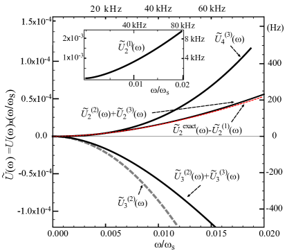
Figure 2: (Color Online) Perturbative predictions for dimensionless effective interaction energies $\tilde{U}_{m}(\omega)$ versus $\omega/\omega_{\text{s}}$ for fixed scattering length $a_{\text{t}}(0),$ in units of the energy $\hbar\omega_{\text{s}}=\hbar^{2}/m_{\text{A}}[a_{\text{t}}(0)]^{2}.$ The inset shows the first-order two-body energy $\tilde{U}_{2}^{(1)}(\omega).$ The main figure shows the second- and third-order corrections to the two-, three-, and four-body energies, assuming no finite-range corrections. The top and right axes in both figures show the energies converted to frequency units by multiplying by $\omega_{\text{s}}/2\pi,$ assuming ⁸⁷Rb with $a_{\text{t}}(0)=5.3$ nm, $m_{\text{A}}=86.9$ u, and $\omega_{\text{s}}/2\pi=4.14$ MHz. The line labeled $\tilde{U}_{2}^{\text{exact}}(\omega)-\tilde{U}_{2}^{(1)}(\omega)$ gives values using the exact two-body results for $\tilde{U}_{2}(\omega)$ from Busch et al. (1998).

III Comparison of perturbative energies with energies for finite-range interactions

This section compares the predictions of the perturbative ground-state energies for a zero-range $\delta$-function interaction potential, summarized in Sec. II and derived in Secs. IV and V, and numerically obtained energies for $N$-boson systems with finite-range interactions. We show that the leading-order contribution of an energy-dependent pseudopotential accurately captures the finite-range effects, and allows us to also validate the analytic and numerical coefficients found from the zero-range perturbation theory.

We use a finite-range interaction model based on a Gaussian two-body potential $V_{\text{g}}(r)=V_{0}\exp[-(r/r_{0})^{2}/2]$ with depth (or height) $V_{0}$ and width $r_{0}$ von Stecher et al. (2008); Suzuki and Varga (1998). For a given width $r_{0}$, we adjust the depth $V_{0}$ such that $V_{\text{g}}(r)$ produces the physical free-space $s$-wave scattering length $a_{\text{t}}(0)$ at zero collision energy. We restrict ourselves to depths $V_{0}$ for which $V_{\text{g}}$ supports no two-body $s$-wave bound state in free-space. This implies that $V_{0}$ is positive for $a_{\text{t}}(0)>0$ and negative for $a_{\text{t}}(0)<0$.

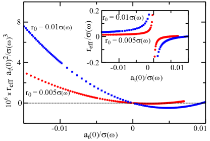
Figure 3: (Color online) Free-space scattering quantities for the Gaussian model potential, with all lengths expressed in units of $\sigma(\omega).$ Circles and squares show the volume $r_{\text{eff}}[a_{\text{t}}(0)]^{2}/[\sigma(\omega)]^{3}$ (in the main figure) and the effective range $r_{\text{eff}}/\sigma(\omega)$ (in the inset) as a function of $a_{\text{t}}(0)/\sigma(\omega)$ for the Gaussian potential with $r_{0}=0.005\sigma(\omega)$ and $r_{0}=0.01\sigma(\omega)$, respectively.

An energy-dependent free-space scattering length for two particles with relative energy $E_{\text{rel}}$ and relative wave number $k_{\text{rel}}=\sqrt{m_{\text{A}}E_{\text{rel}}}/\hbar$ can be defined as

$$a_{\text{f}}(E_{\text{rel}})=-\frac{\tan(\delta_{\text{f}}(k_{\text{rel}}))}{k_{\text{rel}}},$$ (17)

where $\delta_{\text{f}}(k_{\text{rel}})$ is the free-space $s$-wave phase shift. The effect of a finite-range potential on the free-space scattering of two ultracold bosons can be captured by Taylor-expanding $\delta_{\text{f}}(k_{\text{rel}})$ Taylor (2002); Mott and Massey (1965), giving

$$a_{\text{f}}(E_{\text{rel}})=a_{\text{t}}(0)+\frac{1}{2}r_{\text{eff}}[a_{\text{t}}(0)]^{2}k_{\text{rel}}^{2}+\cdots,$$ (18)

where $r_{\text{eff}}$ is the effective range parameter which describes the lowest-order energy dependence of the phase shift Blume and Greene (2002); Bolda et al. (2002).

Figure 3 shows the effective range $r_{\text{eff }}$ and the “volume” $r_{\text{eff}}[a_{\text{t}}(0)]^{2}$ for two bosons interacting with the Gaussian potential with two different choices of $r_{0}/\sigma(\omega)\ll 1.$ (The volume factor here characterizes the leading-order effective-range correction to $s$-wave scattering.) We extract $r_{\text{eff}}$ by fitting the numerically evaluated $-\tan(\delta_{\text{f}}(k_{\text{rel}}))/k_{\text{rel}}$ to the right-hand-side of Eq. (18) for small scattering energies. The effective range is positive for negative $a_{\text{t}}(0),$ negative for small positive $a_{\text{t}}(0),$ and diverges as $a_{\text{t}}(0)\rightarrow 0$. Importantly, since $a_{\text{t}}(0)=0$ implies $V_{0}=0$ (no scattering potential), the volume $r_{\text{eff}}[a_{\text{t}}(0)]^{2}\$also vanishes when $a_{\text{t}}(0)=0$, as seen in the main part of Fig. 3. The divergent behavior of the effective range is also observed for realistic van der Waals potentials Gao (1998) and indeed for any potential that falls off faster than $1/r^{5}$ Mott and Massey (1965), although for these potentials (unlike the Gaussian) $r_{\text{eff}}[a_{\text{t}}(0)]^{2}$ is finite but non-zero in the limit $a_{\text{t}}(0)\rightarrow 0.$

We determine the ground-state energy of $N=3$ and $N=4$ bosons interacting through the Gaussian model potential under external spherically symmetric harmonic confinement using a basis set expansion that expresses the relative $N$-body wave function in terms of explicitly correlated Gaussians Suzuki and Varga (1998)

$$\psi_{\text{rel}}=\sum_{k=1}^{N_{b}}u_{k}{\mathcal{S}}\exp\left[-\frac{1}{2}\sum_{i<j}\left(\frac{r_{ij}}{v_{ij}^{(k)}}\right)^{2}\right].$$ (19)

The $u_{k}$ denote expansion coefficients, $N_{b}$ is the number of basis functions, and ${\mathcal{S}}$ symmetrizes the wave function under the exchange of any pair of bosons. The $N_{b}\times N(N-1)/2$ variational widths $v_{ij}^{(k)},$ chosen stochastically from the interval $[r_{0}/5,4\sigma(\omega)],$ are optimized semi-stochastically following the scheme outlined in Ref. Suzuki and Varga (1998). In brief, the variational method works as follows. Assume we have a basis set consisting of $j-1$ basis functions that yields a ground-state energy estimate $E_{j-1}$. To add the $j^{th}$ basis function $(j\leq N_{b}$), we generate a few thousand trial functions. For each trial function, we solve for a trial ground-state energy by diagonalizing a $j\times j$ dimensional generalized eigenvalue problem. (It is a generalized eigenvalue problem because the basis functions are nonorthogonal.) We choose as the $j^{th}$ basis function the one which makes $E_{j}$ smallest, and repeat this process for the $(j+1)^{th}$ basis function until $j=N_{b}$. A key benefit of the explicitly correlated basis functions is that the Hamiltonian and overlap matrix elements have compact analytical expressions Suzuki and Varga (1998).

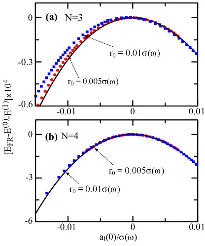
Figure 4: (Color online) The quantity $[E_{\text{FR}}-E^{(0)}-E^{(1)}]\times 10^{4}$ versus $a_{\text{t}}(0)/\sigma(\omega)$ for $N=3$ and $4$ in panel (a) and (b), respectively. (Energies are in units of $\hbar\omega.$) The finite-range energies $E_{\text{FR }}$ are numerically computed with $r_{0}=0.01\sigma(\omega)$ (blue squares) and $r_{0}=0.005\sigma(\omega)$ (red circles). The solid line is $[E^{(2)}+E^{(3)}]\times 10^{4}$ found from the perturbative theory with the zero-range potential.

Convergence is analyzed by investigating the dependence of the energies on $N_{b}$ and by performing calculations for different sets of widths $v_{ij}^{(k)}$. To meaningfully compare numerical three- and four-body energies $E_{\text{FR}}$ for the finite-range (FR) interaction potential with perturbative results up to order $[a_{\text{t}}(0)]^{3}$, the numerical accuracy of the finite-range energies should be notably better than $|a_{\text{t}}(0)/\sigma(\omega)|^{3}$. For example, for $|a_{\text{t}}(0)|=0.001\sigma(\omega)$ and $|a_{\text{t}}(0)|=0.01\sigma(\omega),$ this implies numerical accuracy better than $10^{-9}$ and $10^{-6}$, respectively. An analysis of the basis set error shows that our $N$-body energies are sufficiently accurate to test the perturbative predictions up to order $[a_{\text{t}}(0)]^{3}$ for $|a_{\text{t}}(0)|\gtrsim 0.1r_{0},$ using about $100$ and $500$ basis functions for $N=3$ and $N=4$, respectively. Our numerical accuracy is insufficient to test the perturbative predictions for smaller $|a_{\text{t}}(0)|$.

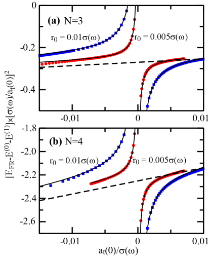
Figure 5: (Color online) Analysis of the three-boson [panel (a)] and four-boson [panel (b)] energies including scattering length and effective range effects. All energies are scaled by $[\sigma(\omega)/a_{\text{t}}(0)]^{2}$ to emphasize the corrections due to finite range effects. The numerically determined finite-range energies $E_{\text{FR}}$ are calculated for the Gaussian potential with spatial width $r_{0}=0.005\sigma(\omega)$ (red circles) and $r_{0}=0.010\sigma(\omega)$ (blue squares), respectively. The dashed line shows the scaled perturbation theory prediction $E^{(2)}+E^{(3)}$ for a zero-range, delta-function potential. The divergence at $a_{\text{t}}(0)/\sigma(\omega)=0$ is due to the divergence of the effective range at zero scattering length. The unscaled energy shift vanishes when $a_{\text{t}}(0)=0.$ The solid lines show the scaled energies $E^{(2)}+E^{(3)}+E^{(1,2)},$ which include the perturbatively calculated finite-range correction $E^{(1,2)}$.

Figure 4 shows the quantity $[E_{\text{FR}}-E^{(0)}-E^{(1)}]\times 10^{4}$ versus $a_{\text{t}}(0)/\sigma(\omega),$ with the finite-range energies $E_{\text{FR }}$ numerically computed using $r_{0}=0.01\sigma(\omega)$ (the blue squares) and $r_{0}=0.005\sigma(\omega)$ (the red circles). We have subtracted the energies $E^{(0)}$ and $E^{(1)}$ obtained from the perturbative theory to better examine the physics beyond first order in $a_{\text{t}}(0).$ The solid line is $[E^{(2)}+E^{(3)}]\times 10^{4}$ from the perturbative theory with $r_{\text{eff}}=0$. Panels (a) and (b) give the energies for $N=3$ and $4$ bosons, respectively. For $N=3,$ we see that finite-range corrections to the zero-range theory become more significant for increasing $r_{0}.$

In Figs. 5(a) and (b), we multiply the $N=3$ and $4$ energies $E_{\text{FR}}-E^{(0)}-E^{(1)}$ by $[\sigma(\omega)/a_{\text{t}}(0)]^{2}$. The perturbative predictions for $(E^{(2)}+E^{(3)})[\sigma(\omega)/a_{\text{t}}(0)]^{2}$ are straight lines. The nonperturbative numerical results are for potentials with $r_{0}=0.005\sigma(\omega)$ and $r_{0}=0.01\sigma(\omega)$. The figures show that the scaled numerical results are singular near zero scattering length, and only approach the zero-range perturbative results with increasing $|a_{\text{t}}(0)|.$ Moreover, by decreasing $r_{0}$ the difference between the perturbative results and the scaled finite-range energies is reduced, and we conclude that the divergences at $a_{\text{t}}(0)=0$ are due to the finite range of the Gaussian potential. Multiplying the energies by $[\sigma(\omega)/a_{\text{t}}(0)]^{2}$ has magnified the finite-range corrections, showing that an effective field theory description for finite-range potentials requires corrections to the zero-range $\delta$-function potential.

We can calculate the leading-order influence of a finite-range potential by including the energy-dependent zero-range pseudopotential of Eq. (5). For the $N$-boson ground state, the pseudopotential gives to first order in $g_{2}^{\prime}$ an energy shift $E^{(1,2)}$ [see Eq. (7)]. At this order, the addition of $\mathcal{V}_{2}^{\prime}$ is equivalent to replacing $a_{\text{t}}(0)\$by $a_{\text{f}}(E_{\text{rel}})$, with Eq. (18) evaluated at the relative zero-point energy $E_{\text{rel}}=3/2$ (in units of $\hbar\omega$) of two non-interacting bosons in the trap.

The solid lines in Fig. 5 show $(E^{(2)}+E^{(3)}+E^{(1,2)})[\sigma(\omega)/a_{\text{t}}(0)]^{2}$ as a function of $a_{\text{t}}(0)/\sigma(\omega)$ for $N=3$ and $N=4$ trapped bosons, respectively. Combining the perturbative predictions for zero-range contributions $E^{(2)}+E^{(3)}$ and the effective-range correction $E^{(1,2)}$ gives excellent agreement with the nonperturbative finite-range energies. The comparison validates the perturbation theory and predictions derived in this paper for effective interactions including finite-range corrections, through third order in $a_{\text{t}}(0)$. It also shows that the divergences in Fig. 5 at $a_{\text{t}}(0)=0$ are due to the divergence of the effective range shown in the inset of Fig. 3. Finally, we note that the energy shift is proportional to the volume $r_{\text{eff}}[a_{\text{t}}(0)]^{2}$ and goes to zero at $a_{\text{t}}(0)=0,$ as expected.

IV First- and second-order effective interactions

IV.1 Hamiltonian and renormalization condition

The numerical results in Sec. III show that finite-range effects are important at third order in perturbation theory for realistic bosons. We incorporate these corrections by modeling the pairwise collisions of ultracold bosons by combining the zero-range pseudopotential

$$\mathcal{V}_{2}(\mathbf{r}_{1}-\mathbf{r}_{2})=4\pi\frac{\hbar^{2}}{m_{\text{A}}}a_{\text{bare}}\delta^{(3)}(\mathbf{r}_{1}-\mathbf{r}_{2}),$$ (20)

where $a_{\text{bare}}$ is now identified as the bare scattering length, and the effective-range potential

$$\mathcal{V}_{2}^{\prime}(\mathbf{r}_{1}-\mathbf{r}_{2})=-\frac{1}{2}g_{2,\text{bare}}^{\prime}\\ \times[\overleftarrow{\nabla}_{12}^{2}\delta^{(3)}(\mathbf{r}_{1}-\mathbf{r}_{2})+\delta^{(3)}(\mathbf{r}_{1}-\mathbf{r}_{2})\overrightarrow{\nabla}_{12}^{2}],$$ (21)

which has the bare coupling constant

$$g_{2,\text{bare}}^{\prime}=\left(4\pi\frac{\hbar^{2}}{m_{\text{A}}}\right)\left(\frac{1}{2}r_{\text{eff}}[a_{\text{bare}}]^{2}\right).$$ (22)

The interactions of $N$ ultracold neutral bosons can be described in quantum field theory with the Hamiltonian $\mathcal{H}=\mathcal{H}_{0}+\mathcal{H}_{\text{I}},$ where $\mathcal{H}_{0}$ is the single-particle Hamiltonian and

$$\mathcal{H}_{\text{I}}=\frac{1}{2}\int\hat{\psi}^{{\dagger}}(\mathbf{r}_{1})\hat{\psi}^{{\dagger}}(\mathbf{r}_{2})[\mathcal{V}_{2}(\mathbf{r}_{1}-\mathbf{r}_{2})\\ +\mathcal{V}_{2}^{\prime}(\mathbf{r}_{1}-\mathbf{r}_{2})]\hat{\psi}(\mathbf{r}_{1})\hat{\psi}(\mathbf{r}_{2})d\mathbf{r}_{1}d\mathbf{r}_{2}.$$ (23)

The field operators $\hat{\psi}(\mathbf{r)}$ and $\hat{\psi}^{{\dagger}}(\mathbf{r)}$ respectively annihilate and create a boson at position $\mathbf{r}$. We assume the absence of intrinsic three- or higher-body interactions.

The bosonic field is expanded over isotropic harmonic oscillator states with frequency $\omega$ as

$$\hat{\psi}(\mathbf{r)}=\sum_{nlm}\phi_{nlm}(\mathbf{r)}\hat{a}_{nlm}=\sum_{i}\phi_{i}(\mathbf{r)}\hat{a}_{i},$$ (24)

with $\hat{a}_{i}$ annihilating a boson in orbital $\phi_{i}(\mathbf{r)}.$ In the following we use the shorthand notation $i=\{nlm\}$, denoting the (dimensionless) single-particle energies as $\varepsilon_{i}=\varepsilon_{nlm}=(2n+l+3/2),$ where $n,l=0,1,2,...,$ and $i=0$ is the $\{nlm\}=\{000\}$ single-particle vibrational ground state. Substituting Eq. (24) into $\mathcal{H}$ and dividing by $\hbar\omega,$ we define the dimensionless Hamiltonian $H=H_{0}+H_{\text{I}}+H_{\text{I}}^{\prime},$ where $H_{0}=\sum_{i}\varepsilon_{i}\hat{a}_{i}^{{\dagger}}\hat{a}_{i},$

$$H_{\text{I}}=\frac{1}{2}\left(\frac{a_{\text{bare}}}{\sigma(\omega)}\right)\sum_{ijkl}K_{ij;kl}\hat{a}_{i}^{{\dagger}}\hat{a}_{j}^{{\dagger}}\hat{a}_{k}\hat{a}_{l},$$ (25)

and

$$H_{\text{I}}^{\prime}=\frac{1}{2}\left(\frac{1}{2}\frac{r_{\text{eff}}[a_{\text{bare}}]^{2}}{\sigma(\omega)^{3}}\right)\sum_{ijkl}K_{ij;kl}^{\prime}\hat{a}_{i}^{{\dagger}}\hat{a}_{j}^{{\dagger}}\hat{a}_{k}\hat{a}_{l}.$$ (26)

The matrix elements

$$K_{ij;kl}=4\pi[\sigma(\omega)]^{3}\int\phi_{i}^{\ast}(\mathbf{r)}\phi_{j}^{\ast}(\mathbf{r)}\phi_{k}(\mathbf{r)}\phi_{l}(\mathbf{r)}d\mathbf{r}$$ (27)

and

$$K_{ij;kl}^{\prime}=-4\pi[\sigma(\omega)]^{5}\int[\phi_{i}^{\ast}(\mathbf{r})\phi_{j}^{\ast}(\mathbf{r})]\overleftrightarrow{\nabla}_{\mathbf{r}}^{2}[\phi_{k}(\mathbf{r})\phi_{l}(\mathbf{r})]d\mathbf{r}$$ (28)

are normalized such that $K_{00;00}=\sqrt{2/\pi}$ and $K_{00;00}^{\prime}=(3/4)\sqrt{2/\pi},$ with the semi-colon separating initial and final states and $\overleftrightarrow{\nabla}_{\mathbf{r}}^{2}=(\overleftarrow{\nabla}_{\mathbf{r}}^{2}+\overrightarrow{\nabla}_{\mathbf{r}}^{2})/2.$ The factors of $[\sigma(\omega)]^{3}$ and $[\sigma(\omega)]^{5}$ make the matrix elements dimensionless and $\omega$-independent. As explained in Sec. II, we assume a regime where $H_{\text{I}}^{\prime}$ can be treated as third order in perturbation theory.

The noninteracting ground state containing $N$ bosons in the $i=0$ (i.e., $nlm=000$) vibrational ground state is $|N\rangle=\hat{a}_{0}^{{\dagger}N}|0\rangle/\sqrt{N!}$, with energy $E^{(0)}=N\varepsilon_{0}$ and $\varepsilon_{0}=3/2.$ First-order perturbation theory in $H_{\text{I}}$ gives $E^{(1)}(\omega)=(1/2)N(N-1)U_{2}^{(1)}$ with

$$U_{2}^{(1)}=\alpha_{2}^{(1)}\left(\frac{a_{\text{bare}}}{\sigma(\omega)}\right),$$ (29)

using $\left\langle N\right|a_{0}^{{\dagger}}a_{0}^{{\dagger}}a_{0}a_{0}\left|N\right\rangle=N(N-1)$ and recalling that $|N\rangle$ denotes $N$ bosons in the non-interacting vibrational state $nlm=000.$ The two-body, first-order coefficient is $\alpha_{2}^{(1)}=\sqrt{2/\pi}.$

At higher orders in $H_{\text{I}},$ there are divergences due to the $\delta$-function potential (see e.g. Huang and Yang (1957); Fetter and Walecka (1971)). We regulate these by either truncating sums over intermediate states at a high-energy cutoff $\hbar\omega_{c},$ or by using an exponential regulator function. The former is more convenient for numerical approximations, while the latter is more convenient for analytic results. In either case, we find at second order that $U_{2}^{(2)}$ diverges as $\sqrt{\omega_{c}}$ and renormalization is required. Although this can be done using bare perturbation theory, in which infinities are absorbed by appropriately redefining bare parameters, we use the method of renormalized perturbation theory which provides a systematic and self-consistent approach for calculations beyond second order involving multiple divergent terms.

Renormalized perturbation theory (e.g., see Srednicki (2007)) re-expresses the bare scattering length as

$$a_{\text{bare}}=a_{\text{t}}(\omega_{0})+a_{\text{ct}}(\omega_{0}).$$ (30)

A renormalization condition defines $a_{\text{t}}(\omega_{0})$ as the physical scattering length for two bosons in a trap at frequency $\omega_{0}$. The cutoff dependent remainder $a_{\text{ct}}(\omega_{0})$ is called a counterterm. For brevity, this notation suppresses the dependence of $a_{\text{ct}}(\omega_{0})$ on $\omega_{c}$. In the following, we call $a_{\text{t}}(\omega_{0})$ the “trap scattering length” at frequency $\omega_{0},$ to distinguish it from the energy-dependent free-space scattering length $a_{\text{f}}(E_{\text{rel}}$) defined in Eq. (17). In the limits of zero relative collision energy and $\omega_{0}=0,$ the trap and free-space scattering lengths are equal, i.e., $a_{\text{t}}(0)=a_{\text{f}}(0).$ With the combination of $\mathcal{V}_{2}$ and $\mathcal{V}_{2}^{\prime},$ the trap scattering length $a_{\text{t}}(\omega_{0})$ includes both the effects of the $\omega_{0}$-dependent dressing by quantum fluctuations to higher orbitals and finite-range effects. Note that the trap scattering length $a_{\text{t}}(\omega_{0})\$does not, in general, equal the free-space scattering length $a_{\text{f}}(E_{\text{rel}})$ defined in Eq. (18) because the latter does not correctly capture the influence of the harmonic confinement on the quantum fluctuations to higher orbitals.

Together with the renormalization condition, the other key ingredient in renormalized perturbation theory is that the leading-order scattering length counterterm $a_{\text{ct}}(\omega_{0})$ is proportional to $[a_{\text{t}}(\omega_{0})]^{2};$ in other words, it is a second- and higher-order contribution. This, plus the renormalization condition, systematically reorganizes the perturbation theory, order-by-order, so that it is an expansion in the physical value $a_{\text{t}}(\omega_{0})$ instead of $a_{\text{bare}}.$ Figure 6 summarizes the relationship between the characteristic length and energy scales for our model system of trapped ultracold bosons.

Figure 6: The length scales of interacting, harmonically trapped, ultracold bosons. We assume a separation of length scales $l_{c}\ll a_{\text{t}}(\omega_{0})\ll\sigma(\omega_{0}),$ or equivalently a separation of energy scales $\omega_{c}\gg\omega_{\text{s}}\gg\omega_{0},$ where $\omega_{\text{s}}=\hbar/m_{\text{A}}a_{\text{t}}(\omega_{0})^{2}.$ The harmonic oscillator lengths $\sigma(\omega)$ and $\sigma(\omega_{0})$ are of the same order, although $\sigma(\omega_{0})$ is not necessarily larger than $\sigma(\omega)$. Similarly, we assume that $a_{\text{t}}(\omega_{0}),$ $a_{\text{t}}(0),$ $r_{\text{eff}}$, and the Gaussian width $r_{0}$ are of the same order. The order of length scales within a group is arbitrary.

Substituting Eq. (30) into Eqs. (25) and (26) gives

$$H_{\text{I}}(\omega;\omega_{0})=V(\omega;\omega_{0})+V^{\prime}(\omega;\omega_{0})+V_{\text{ct}}(\omega;\omega_{0}),$$ (31)

where the zero-range and counterterm operators are

$$V(\omega;\omega_{0})=\frac{1}{2}\left(\frac{a_{\text{t}}(\omega_{0})}{\sigma(\omega)}\right)\sum_{ijkl}K_{ij;kl}\hat{a}_{i}^{{\dagger}}\hat{a}_{j}^{{\dagger}}\hat{a}_{k}\hat{a}_{l},$$ (32)

$$V_{\text{ct}}(\omega;\omega_{0})=\frac{1}{2}\left(\frac{a_{\text{ct}}(\omega_{0})}{\sigma(\omega)}\right)\sum_{ijkl}K_{ij;kl}\hat{a}_{i}^{{\dagger}}\hat{a}_{j}^{{\dagger}}\hat{a}_{k}\hat{a}_{l},$$ (33)

and the effective-range operator is

$$V^{\prime}(\omega;\omega_{0}) =\frac{1}{2}\left(\frac{1}{2}\frac{r_{\text{eff}}[a_{\text{t}}(\omega_{0})]^{2}}{[\sigma(\omega)]^{3}}\right)\sum_{ijkl}K_{ij;kl}^{\prime}\hat{a}_{i}^{{\dagger}}\hat{a}_{j}^{{\dagger}}\hat{a}_{k}\hat{a}_{l}$$

$$+\mathcal{O}\left(\frac{r_{\text{eff}}[a_{\text{t}}(0)]^{3}}{[\sigma(\omega)]^{4}}\right).$$ (34)

The renormalized perturbation theory is then organized based on the observation that $V(\omega;\omega_{0})$ is proportional to $a_{\text{t}}(\omega_{0})$, $V_{\text{ct}}(\omega;\omega_{0})$ is proportional to $[a_{\text{t}}(\omega_{0})]^{2}$, and $V^{\prime}(\omega;\omega_{0})$ is (for the regime considered here) proportional to $[a_{\text{t}}(\omega_{0})]^{3}.$ The single counterterm operator $V_{\text{ct}}(\omega;\omega_{0})$ cancels all divergences from the operator $V(\omega;\omega_{0}),$ at all orders in perturbation theory. In contrast, the effective-range operator $V^{\prime}(\omega;\omega_{0})$ leads to a nonrenormalizable field theory with the consequence that new counterterm operators are required at every order in perturbation theory beyond first order in $g_{2}^{\prime}$; because we are only working to first order in $g_{2}^{\prime}$ in this paper, no additional counterterms are needed.

Note that the frequency $\omega_{0}$ at which $a_{\text{t}}(\omega_{0})$ is defined and the trap frequency $\omega$ for which we want to compute energies are independent. In the overview, we summarized our results for the special case where $\omega_{0}=0$. The general case of arbitrary $\omega_{0}$ facilitates renormalization of the perturbation theory. More importantly, the renormalized perturbation theory is “calibrated” to a measured value of $a_{\text{t}}(\omega_{0})$ at a desired trap frequency $\omega_{0}$, and is then used to predict energies for trap frequencies $\omega$ not generally equal to $\omega_{0}.$

We can now compute the ground-state energy

$$E(\omega;\omega_{0}) =\varepsilon_{0}N+\frac{1}{2!}U_{2}(\omega;\omega_{0})N(N-1)$$ (35)

$$+\frac{1}{3!}U_{3}(\omega;\omega_{0})N(N-1)(N-2)$$

$$+\frac{1}{4!}U_{4}(\omega;\omega_{0})N(N-1)(N-2)(N-3)+....$$

We have used the semi-colon notation in Eqs. (31), (32), (33), (34), and (35) to distinguish between the roles of the frequencies $\omega$ and $\omega_{0}$. Before renormalization, the interaction energies $U_{m}(\omega;\omega_{0})$, found from perturbation theory in $H_{\text{I}}(\omega;\omega_{0}),$ are functions of $a_{\text{t}}(\omega_{0})$ and $a_{\text{ct}}(\omega_{0}).$ The renormalization condition can be expressed as

$$U_{2}(\omega=\omega_{0};\omega_{0})=\sqrt{\frac{2}{\pi}}\left(\frac{a_{\text{t}}(\omega_{0})}{\sigma(\omega=\omega_{0})}\right),$$ (36)

which, in practice, is solved for $a_{\text{ct}}(\omega_{0})$ to the desired order in perturbation theory. Another way of describing the renormalization condition is that $a_{\text{ct}}(\omega_{0})$ is tuned such that the first-order result is exact and the second- and higher-order corrections to the two-body energy vanish when evaluated for two bosons in a trap with $\omega=\omega_{0}.$ After renormalization, the interaction energies $U_{m}(\omega;\omega_{0})$ depend only on $a_{\text{t}}(\omega_{0})$ and, moreover, the $\omega$-dependence of the ground-state energy satisfies $E(\omega;\omega_{0})=E(\omega;\omega_{0}^{\prime}),$ for any pair of frequencies $\omega_{0}$ and $\omega_{0}^{\prime}.$

IV.2 Energy at first-order in scattering length

We use renormalized Rayleigh-Schrödinger (RS) perturbation theory to compute the $N$-boson ground-state energy $E=\sum_{n=0}E^{(n)},$ where $E^{(n)}$ is proportional to $[a_{\text{t}}(\omega_{0})]^{n}$. We separate the contributions at each order into $m$-body energies, such that $U_{m}(\omega;\omega_{0})=\sum_{n}U_{m}^{(n)}(\omega;\omega_{0})$. The zeroth-order term is $E^{(0)}(\omega)=\varepsilon_{0}N$. The first-order energy shift is

$$E^{(1)}(\omega;\omega_{0}) =\langle N|H_{\text{I}}(\omega;\omega_{0})|N\rangle=\langle N|V(\omega;\omega_{0})|N\rangle$$

$$=\frac{1}{2}\sqrt{\frac{2}{\pi}}\left(\frac{a_{\text{t}}(\omega_{0})}{\sigma(\omega)}\right)N(N-1),$$ (37)

using the fact that $V$, $V_{\text{ct}},$ and $V^{\prime}$ are $\mathcal{O}(a_{\text{t}}(\omega_{0})/\sigma(\omega))$, $\mathcal{O}([a_{\text{t}}(\omega_{0})/\sigma(\omega)]^{2})$, and $\mathcal{O(}[a_{\text{t}}(\omega_{0})/\sigma(\omega)]^{3}),$ respectively, and $\left\langle N\right|a_{0}^{{\dagger}}a_{0}^{{\dagger}}a_{0}a_{0}\left|N\right\rangle=N(N-1)$.

Comparing to Eq. (35), we see that the two-body energy to first-order for any $\omega$ and $\omega_{0}$ is

$$U_{2}^{(1)}(\omega;\omega_{0})=c_{2}^{(1)}\left(\frac{a_{\text{t}}(\omega_{0})}{\sigma(\omega)}\right),$$ (38)

with

$$c_{2}^{(1)}=\alpha_{2}^{(1)}=\sqrt{\frac{2}{\pi}}.$$ (39)

For a trap with $\omega=\omega_{0},$ the renormalization condition says that $U_{2}^{(1)}(\omega_{0};\omega_{0})=\sqrt{2/\pi}[a_{\text{t}}(\omega_{0})/\sigma(\omega_{0})]$ is the exact two-body energy. For $\omega\neq\omega_{0},$ $U_{2}^{(1)}(\omega\neq\omega_{0};\omega_{0})$ is the leading order contribution to the full two-body energy $U_{2}(\omega;\omega_{0}),$ but, as shown in the following sections, there are higher-order corrections that become increasingly important the more $\omega$ differs from $\omega_{0}.$

IV.3 Energy at second-order in scattering length

The second-order energy shift is given by

$$E^{(2)}=V_{\text{ct;}00,00}-\sum_{ij\neq 00}^{\omega_{c}/\omega}\frac{V_{00,ij}V_{ij,00}}{\Delta\varepsilon_{ij}},$$ (40)

where $V_{ij,kl}=\langle ij|V|kl\rangle$ and $V_{\text{ct;}ij,kl}=\langle ij|V_{\text{ct}}|kl\rangle.$ The notation $|ij\rangle=Z_{ij}\hat{a}_{i}^{{\dagger}}\hat{a}_{j}^{{\dagger}}\hat{a}_{0}\hat{a}_{0}\left|N\right\rangle$ denotes the state with either one or two particles excited from the non-interacting ground state, $\Delta\varepsilon_{ij}=\varepsilon_{i}+\varepsilon_{j}-2\varepsilon_{0},$ $Z_{ij}$ is a normalization factor, and $ij\neq 00$ denotes summing over all $i,j$ except $i=j=0$. Equation (40) is modified from the usual RS perturbation theory because of the presence of the $\mathcal{O}([a_{\text{t}}(\omega_{0})]^{2})$ interaction term $V_{\text{ct}},$ which generates the counterterm contribution.

The sums over intermediate states $\left|ij\right\rangle$ exclude the ground state $i=j=0$, and are regularized using either a hard cutoff $\Delta\varepsilon_{ij}<\omega_{c}/\omega,$ or an exponential regulator $\Delta\varepsilon_{ij}^{-1}\rightarrow e^{-\Delta\varepsilon_{ij}\omega/\omega_{c}}\Delta\varepsilon_{ij}^{-1},$ where $\hbar\omega_{c}$ is a high-energy cutoff. In the limit $\omega_{c}/\omega\rightarrow\infty,$ these regulators are equivalent.

Using Eqs. (32) and (33), we have

$$E^{(2)}(\omega;\omega_{0})=\frac{1}{2}\alpha_{2}^{(1)}\left(\frac{a_{\text{ct}}(\omega_{0})}{\sigma(\omega)}\right)N(N-1)$$ (41)

$$-\frac{N(N-1)}{4}\left(\frac{a_{\text{t}}(\omega_{0})}{\sigma(\omega)}\right)^{2}\sum_{ij\neq 00,kl}^{\omega_{c}/\omega}\frac{K_{00;ij}K_{kl;00}}{\Delta\varepsilon_{ij}}\langle\hat{a}_{i}\hat{a}_{j}\hat{a}_{k}^{\dagger}\hat{a}_{l}^{\dagger}\rangle,$$

and the expectation value is with respect to the non-interacting ground state $|N-2\rangle\propto\hat{a}_{0}\hat{a}_{0}|N\rangle$. The notation $ij\neq 00,kl$ indicates that the sum is over all $i,j,k,l$ except $i=j=0.$ Wick’s theorem gives

$$\langle\hat{a}_{i}\hat{a}_{j}\hat{a}_{k}^{\dagger}\hat{a}_{l}^{\dagger}\rangle =4\langle\text{:}\contraction{}{\hat{a}}{{}_{a}\hat{a}_{b}}{\hat{a}}\hat{a}_{i}\hat{a}_{j}\hat{a}_{k}^{{\dagger}}\hat{a}_{l}^{{\dagger}}\text{:}\rangle+2\langle\text{:}\contraction{}{\hat{a}}{{}_{a}\hat{a}_{b}}{\hat{a}}\contraction[2ex]{\hat{a}_{a}}{\hat{a}}{{}_{b}\hat{a}_{c}^{{\dagger}}}{\hat{a}}\hat{a}_{i}\hat{a}_{j}\hat{a}_{k}^{{\dagger}}\hat{a}_{l}^{{\dagger}}\text{:}$$

$$=4\delta_{ik}(N-2)+2\delta_{ik}\delta_{jl},$$ (42)

where :: denotes normal ordering, uncontracted indices are set to zero, and contractions $\contraction{}{\hat{a}}{{}_{a}}{\hat{a}}\hat{a}_{i}\hat{a}_{k}^{{\dagger}}=\delta_{ik}$. Also, we have used $\langle$:$\hat{a}_{i}\hat{a}_{j}\hat{a}_{k}^{{\dagger}}\hat{a}_{l}^{{\dagger}}$:$\rangle=0$, $\langle$:$\hat{a}_{0}^{{\dagger}M}\hat{a}_{0}^{M}$:$\rangle=(N-2)(N-3)...(N-M+1),$ and combined equivalent terms. Because of the factor $N-2,$ the first term of Eq. (42) can be understood as leading to an effective three-body interaction, whereas the second term is a correction to the two-body interaction.

The second-order interaction energies $U_{2}^{(2)}(\omega;\omega_{0})$ and $U_{3}^{(2)}(\omega;\omega_{0})$ can be extracted by evaluating Eq. (41) and comparing with Eq. (35). This gives

$$U_{2}^{(2)}(\omega;\omega_{0}) =\alpha_{2}^{(1)}\left(\frac{a_{\text{ct}}(\omega_{0})}{\sigma(\omega)}\right)-\beta_{2}^{(2)}(\omega)\left(\frac{a_{\text{t}}(\omega_{0})}{\sigma(\omega)}\right)^{2}$$

$$=\raisebox{-3.61371pt}{\includegraphics{counterterm1small}}-\raisebox{-3.61371pt}{\includegraphics{alpha1small}},$$ (43)

and

$$U_{3}^{(2)}(\omega;\omega_{0})=-6\alpha_{3}^{(2)}\left(\frac{a_{\text{t}}(\omega_{0})}{\sigma(\omega)}\right)^{2}=-6\raisebox{-3.61371pt}{\includegraphics{beta1small}}.$$ (44)

The expressions for $\beta_{2}^{(2)}(\omega)$ and $\alpha_{3}^{(2)}$ are defined in Table 2, which also shows the explicit values calculated in Appendices A and B for an isotropic harmonic trap. We use the notation that $\alpha_{m}^{(n)}$ and $\beta_{m}^{(n)}(\omega)$ are associated with $n^{\text{th}}$-order, $m$-body processes. The sum that gives $\beta_{2}^{(2)}(\omega)$ diverges with cutoff as $\sqrt{\omega_{c}/\omega}$, where $\omega_{c}/\omega$ is approximately the number of harmonic oscillator levels included in the sum as a function of $\omega,$ for a fixed cutoff $\omega_{c}.$ The coefficient $\alpha_{3}^{(2)}$ is convergent and in the limit $\omega_{c}/\omega\rightarrow\infty$ is independent of $\omega.$ In the following, we only indicate the explicit $\omega$ dependence for coefficients that remain sensitive to $\omega$ in the limit $\omega_{c}/\omega\rightarrow\infty,$ e.g., we write $\beta_{2}^{(2)}(\omega)$ but $\alpha_{3}^{(2)}.$ We use a hard cutoff to numerically evaluate the coefficients $\alpha_{3}^{(3)},\alpha_{4,1}^{(3)}$ and $\alpha_{4,1}^{(3)}$ (see Sec. V for the definitions of the third-order coefficients.) For the coefficients $\alpha_{3}^{(2)},\alpha_{4,3}^{(3)},$ and $\alpha_{5}^{(3)},$ we find analytic results in the limit $\omega_{c}/\omega\rightarrow\infty.$ Finally, using the exponential regulator, we obtain analytic results for the coefficients $\beta_{2}^{(2)}(\omega),\beta_{2}^{(3)}(\omega),$ and $\beta_{3}^{(3)}(\omega)$ for any $\omega_{c}/\omega.$

Equations (43) and (44) have also been represented diagrammatically, with factors of $K_{ij;kl}[a_{\text{t}}(\omega_{0})/\sigma(\omega)]$ assigned vertices , and contractions $\contraction{}{\hat{a}}{{}_{a}}{\hat{a}}\hat{a}_{i}\hat{a}_{k}^{{\dagger}}$ representing excited particles assigned dashed lines $\raisebox{1.4457pt}{\includegraphics{intermediatestate}}.$ Uncontracted operators $\hat{a}_{0}$ (or $\hat{a}_{0}^{{\dagger}}$) are assigned incoming (or outgoing ) lines. The counterterm is represented as $K_{ij;kl}[a_{\text{ct}}(\omega_{0})/\sigma(\omega)]=\raisebox{-3.61371pt}{\includegraphics{counterterm1dashed}}.$ Intermediate states have one or more excited particles and contribute an energy denominator $1/\Delta\varepsilon_{ij}$. For example, the diagram is a graphical representation for the term $\alpha_{3}^{(2)}[a_{\text{t}}(\omega_{0})/\sigma(\omega)]^{2}$, and $U_{3}^{(2)}(\omega;\omega_{0})=-6\raisebox{-3.61371pt}{\includegraphics{beta1small}}.$ We obtain combinatorial prefactors [e.g. $-6$ for $U_{3}^{(2)}\left(\omega,\omega_{0}\right)$] from Wick’s theorem by counting the number of equivalent contractions, dividing by $2$ for every factor of $a_{\text{t}}(\omega_{0})$ or $a_{\text{ct}}(\omega_{0}),$ and multiplying by $m!$ for an $m$-body term.

The renormalization condition through second order is $U_{2}(\omega;\omega_{0})=U_{2}^{(1)}(\omega_{0};\omega_{0})+U_{2}^{(2)}(\omega_{0};\omega_{0})+\mathcal{O}([a_{\text{t}}(\omega_{0})]^{3})+\mathcal{O}(r_{\text{eff}}[a_{\text{t}}(\omega_{0})]^{2})=U_{2}^{(1)}(\omega_{0};\omega_{0}),$ and hence $U_{2}^{(2)}(\omega_{0};\omega_{0})=0.$ Diagrammatically

$$\raisebox{-3.61371pt}{\includegraphics{counterterm1small}}|_{\omega=\omega_{0}}=\raisebox{-3.61371pt}{\includegraphics{alpha1small}}|_{\omega=\omega_{0}}.$$ (45)

Solving for the counterterm gives

$$a_{\text{ct}}(\omega_{0})=\frac{\beta_{2}^{(2)}(\omega_{0})}{\alpha_{2}^{(1)}}\left(\frac{a_{\text{t}}(\omega_{0})}{\sigma(\omega_{0})}\right)^{2}\sigma(\omega_{0}).$$ (46)

Substituting into Eq. (43) gives

$$U_{2}^{(2)}(\omega;\omega_{0})=c_{2}^{(2)}(\omega,\omega_{0})\left(\frac{a_{\text{t}}(\omega_{0})}{\sigma(\omega)}\right)^{2},$$ (47)

where the function

$$c_{2}^{(2)}(\omega,\omega_{0})=\sqrt{\omega_{0}/\omega}\beta_{2}^{(2)}(\omega_{0})-\beta_{2}^{(2)}(\omega)$$ (48)

can be used for any $\omega.$ (We have used $\sigma(\omega_{0})/\sigma(\omega)=\sqrt{\omega/\omega_{0}}$ above to simplify the expressions.)

The form of the expression for the coefficient $c_{2}^{(2)}\left(\omega,\omega_{0}\right)$ ensures that the divergent terms cancel. For an isotropic harmonic oscillator, we show in App. B.6, using an exponential regulator, that

$$\beta_{2}^{(2)}(\omega)=\left(2/\pi\right)[\sqrt{\omega_{c}/2\omega}-(1-\log 2)]+\mathcal{O}(1/\omega_{c}^{1/2}),$$ (49)

and thus

$$c_{2}^{(2)}(\omega,\omega_{0})=\left(2/\pi\right)(1-\log 2)\left[1-\sqrt{\omega_{0}/\omega}\right].$$ (50)

The renormalization condition is automatically satisfied since $c_{2}^{(2)}(\omega_{0},\omega_{0})=0.$ For the special case when $\omega_{0}=0,$ we find

$$c_{2}^{(2)}(\omega,0)=c_{2}^{(2)}=\left(2/\pi\right)(1-\log 2)=0.19535....$$ (51)

For brevity, we define $c_{m}^{(n)}$ without arguments as the coefficients $c_{m}^{(n)}(\omega,0)$ for the special case when $\omega_{0}=0.$ In this limit, the coefficients $c_{m}^{(n)}$ are independent of $\omega$.

Combining the first- and second-order contributions for the two-body interaction energy gives

$$U_{2}(\omega;\omega_{0}) =c_{2}^{(1)}\left(\frac{a_{\text{t}}(\omega_{0})}{\sigma(\omega)}\right)+c_{2}^{(2)}(\omega,\omega_{0})\left(\frac{a_{\text{t}}(\omega_{0})}{\sigma(\omega)}\right)^{2}$$

$$+\mathcal{O}\left(\frac{[a_{\text{t}}(\omega_{0})]^{3}}{[\sigma(\omega)]^{3}}\right)+\mathcal{O}\left(\frac{r_{\text{eff}}[a_{\text{t}}(\omega_{0})]^{2}}{[\sigma(\omega)]^{3}}\right).$$ (52)

The coefficient $\alpha_{3}^{(2)}$ in Eq. (44) is finite and does not require a regulator. For the three-body interaction energy we obtain

$$U_{3}(\omega;\omega_{0}) =c_{3}^{(2)}\left(\frac{a_{\text{t}}(\omega_{0})}{\sigma(\omega)}\right)^{2}+\mathcal{O}\left(\frac{[a_{\text{t}}(\omega_{0})]^{3}}{[\sigma(\omega)]^{3}}\right)$$

$$+\mathcal{O}\left(\frac{r_{\text{eff}}[a_{\text{t}}(\omega_{0})]^{2}}{[\sigma(\omega)]^{3}}\right),$$ (53)

where $c_{3}^{(2)}=-6\alpha_{3}^{(2)}=-0.85576...$ This value was previously obtained in Johnson et al. (2009), and is also calculated in App. B.1.

V Effective interactions through third order

Figure 7: Sequence of boson-boson interaction induced transitions to higher orbitals. This example generates corrections to the ground state energy that can be viewed as an effective three-body interaction. The process, which involves three interaction vertices, arises at third order in perturbation theory and gives the energy shift $\alpha_{3}^{(3)}[a_{\text{t}}(\omega_{0})/\sigma(\omega)]^{3}$ derived in the text. Links labelled $V_{ij}$ represent intrinsic 2-body interactions between particles $i$ and $j$. Black arrows represent virtual transitions to and from excited orbitals. Solid and dashed lines represent atoms in ground and excited vibrational states, respectively. The diagram on the far right shows the perturbation theory diagram for this process.

We now extend our analysis to third order in the scattering length $a_{\text{t}}(\omega_{0})$. This is necessary to obtain the leading-order effective four-body interaction. Including the counterterm and effective-range interaction, the formula for the third-order energy shift is

$$E^{(3)}(\omega;\omega_{0})=\sum_{ij\neq 00,kl\neq 00}^{\omega_{c}/\omega}\frac{V_{00,ij}V_{ij,kl}V_{kl,00}}{\Delta\varepsilon_{ij}\Delta\varepsilon_{kl}}$$ (54)

$$-V_{00,00}\sum_{ij\neq 00}^{\omega_{c}/\omega}\frac{V_{00,ij}V_{ij,00}}{\Delta\varepsilon_{ij}^{2}}-2\sum_{ij\neq 00}^{\omega_{c}/\omega}\frac{V_{\text{ct;}00,ij}V_{ij,00}}{\Delta\varepsilon_{ij}}+V_{00,00}^{\prime}.$$

The first term on the right-hand-side of Eq. (54) gives

$$\frac{1}{8}\left(\frac{a_{\text{t}}(\omega_{0})}{\sigma(\omega)}\right)^{3}N(N-1)\times\\ \sum_{ij\neq 00,klqr,st\neq 00}^{\omega_{c}/\omega}\frac{K_{00;ij}K_{kl;qr}K_{st;00}}{\Delta\varepsilon_{ij}\Delta\varepsilon_{st}}\langle\hat{a}_{i}\hat{a}_{j}\hat{a}_{k}^{\dagger}\hat{a}_{l}^{\dagger}\hat{a}_{q}\hat{a}_{r}\hat{a}_{s}^{\dagger}\hat{a}_{t}^{\dagger}\rangle,$$ (57)

where the expectation value is with respect to the noninteracting ground state with $(N-2)$ bosons. Applying Wick’s theorem, Eq. (57) expands as

$$\left(\frac{a_{\text{t}}(\omega_{0})}{\sigma(\omega)}\right)^{3}\times\Big{(}\frac{1}{2!}\beta_{2}^{(3)}(\omega)N(N-1)$$ (58)

$$+\frac{1}{3!}[12\alpha_{3}^{(3)}+12\beta_{3}^{(3)}(\omega)]N(N-1)(N-2)$$

$$+\frac{1}{4!}[48\alpha_{4,1}^{(3)}+48\alpha_{4,2}^{(3)}+6\alpha_{4,3}^{(3)}]N(N-1)(N-2)(N-3)$$

$$+\frac{1}{5!}60\alpha_{5}^{(3)}N(N-1)(N-2)(N-3)(N-4)\Big{)}.$$

We find effective two-, three-, and four-body interactions from the terms with four, three, and two contractions, respectively. The zero-contraction term vanishes since $\langle$:$\hat{a}_{i}\hat{a}_{j}\hat{a}_{k}^{\dagger}\hat{a}_{l}^{\dagger}\hat{a}_{i^{\prime}}\hat{a}_{j^{\prime}}\hat{a}_{k^{\prime}}^{\dagger}\hat{a}_{l^{\prime}}^{\dagger}$:$\rangle=0.$ Comparing to Eq. (35), we see that there is a two-body contribution $\beta_{2}^{(3)}(\omega)[a_{\text{t}}(\omega_{0})/\sigma(\omega)]^{3}=\raisebox{-5.00098pt}{\includegraphics{alpha2small}},$ there are two three-body contributions $12\alpha_{3}^{(3)}[a_{\text{t}}(\omega_{0})/\sigma(\omega)]^{3}=12\raisebox{-3.61371pt}{\includegraphics{beta2small}}$ and $12\beta_{3}^{(3)}(\omega)[a_{\text{t}}(\omega_{0})/\sigma(\omega)]^{3}=12\raisebox{-3.61371pt}{\includegraphics{betactsmall}},$ and so on. The definitions for the coefficients $\beta_{2}^{(3)},\alpha_{3}^{(3)},\beta_{3}^{(3)},$ etc., are given in Table 2, along with the associated diagrams, asymptotic behavior, and explicit forms for an isotropic harmonic oscillator potential (calculated in Appendices A and B). Figure 7 illustrates one of the sequences of virtual transitions giving rise to $\alpha_{3}^{(3)}.$

Energies (Diagrams) Coefficients Asymp. Isotropic H.O. coefficients ($\omega_{c}\rightarrow\infty$) 1${}^{\text{st}}$-order in $\xi_{\text{t}}=a_{\text{t}}(\omega_{0})/\sigma(\omega)$ $\alpha_{2}^{(1)}\xi_{\text{t}}$ = $\alpha_{2}^{(1)}=K_{0000}$ N.A. $\sqrt{\frac{2}{\pi}}=+0.797885...$ 2${}^{\text{nd}}$-order in $\xi_{\text{t}}$ $\alpha_{3}^{(2)}\xi_{\text{t}}^{2}$ =  $\alpha_{3}^{(2)}=\sum\frac{K_{000i}K_{i000}}{\Delta\varepsilon_{i0}}$ $a+e^{-\omega_{c}/\omega}$ $\left(\frac{2}{\pi}\right)[\frac{2\sqrt{3}}{3}+\log(8-4\sqrt{3})-1]=+0.142626...$ $\beta_{2}^{(2)}(\omega)\xi_{\text{t}}^{2}$ =  $\beta_{2}^{(2)}=\sum\frac{K_{00ij}K_{ij00}}{\Delta\varepsilon_{ij}}$ $\sqrt{\frac{\omega_{c}}{\omega}}$ $\left(\frac{2}{\pi}\right)[\sqrt{\frac{\omega_{c}}{2\omega}}-(1-\log 2)-\frac{3}{2}\sqrt{\frac{\omega}{2\omega_{c}}}]$ 3${}^{\text{rd}}$-order in $\xi_{\text{t}}$ $\beta_{2}^{(3)}(\omega)\xi_{\text{t}}^{3}$ =  $\beta_{2}^{(3)}=\sum\frac{K_{00ij}K_{ijkl}K_{kl00}}{\Delta\varepsilon_{ij}\Delta\varepsilon_{kl}}$ $\left(\frac{\omega_{c}}{\omega}\right)$ $[\beta_{2}^{(2)}(\omega)]^{2}/\alpha_{2}^{(1)}$ $\beta_{3}^{(3)}(\omega)\xi_{\text{t}}^{3}$ =  $\beta_{3}^{(3)}=\sum\frac{K_{00ij}K_{ij0k}K_{k000}}{\Delta\varepsilon_{ij}\Delta\varepsilon_{k0}}$ $\sqrt{\frac{\omega_{c}}{\omega}}$ $\beta_{2}^{(2)}(\omega)\alpha_{3}^{(2)}/\alpha_{2}^{(1)}$ $\alpha_{3}^{(3)}\xi_{\text{t}}^{3}$ =  $\alpha_{3}^{(3)}=\sum\frac{K_{00ij}K_{j00k}K_{ik00}}{\Delta\varepsilon_{ij}\Delta\varepsilon_{ik}}$ $a+\sqrt{\frac{\omega}{\omega_{c}}}$ $+0.56494\pm 0.00001\$(estimate) $\alpha_{4,1}^{(3)}\xi_{\text{t}}^{3}$ =  $\alpha_{4,1}^{(3)}=\sum\frac{K_{00ij}K_{j000}K_{i000}}{\Delta\varepsilon_{ij}\Delta\varepsilon_{i0}}$ $a+e^{-\omega_{c}/\omega}$ $+0.077465...\$(numerical) $\alpha_{4,2}^{(3)}\xi_{\text{t}}^{3}$ =  $\alpha_{4,2}^{(3)}=\sum\frac{K_{000i}K_{i00j}K_{j000}}{\Delta\varepsilon_{i0}\Delta\varepsilon_{j0}}$ $a+e^{-\omega_{c}/\omega}$ $+0.051099...\$(numerical) $\alpha_{4,3}^{(3)}\xi_{\text{t}}^{3}$ =  i$\alpha_{4,3}^{(3)}=\sum\frac{K_{00ij}K_{0000}K_{ij00}}{\Delta\varepsilon_{ij}^{2}}$ $a+\sqrt{\frac{\omega}{\omega_{c}}}$ $\left(\frac{2}{\pi}\right)^{3/2}[\frac{\pi^{2}}{24}+\log 2-\frac{1}{2}\left(\log 2\right)^{2}]=+0.438946...$ $\alpha_{5}^{(3)}\xi_{\text{t}}^{3}$ =  $\alpha_{5}^{(3)}=\sum\frac{K_{000i}K_{0000}K_{i000}}{\Delta\varepsilon_{i0}{}^{2}}$ $a+e^{-\omega_{c}/\omega}$ $\frac{3}{4(2\pi)^{3/2}}{}_{4}F_{3}\left(1,1,1,5/2;2,2,2;1/4\right)=+0.051916...$ Counterterms through third order $\chi_{\text{ct}}=\frac{a_{\text{ct}}(\omega_{0})}{\sigma(\omega)},$ $\ \alpha_{2}^{(1)}\chi_{\text{ct}}=\raisebox{-5.05942pt}{\includegraphics{counterterm1}},\ \ \ \ \beta_{2}^{(2)}(\omega)\chi_{\text{ct}}\xi_{\text{t}}=\raisebox{-5.05942pt}{\includegraphics{counterterm2}},\ \ \ \ \alpha_{3}^{(2)}\chi_{\text{ct}}\xi_{\text{t}}=\raisebox{-5.05942pt}{\includegraphics{counterterm3}}$ Leading-order effective range terms $\alpha_{2}^{(1,2)}\left(\frac{r_{\text{eff}}}{\sigma(\omega)}\right)\xi_{\text{t}}^{2}=\raisebox{-3.61371pt}{\includegraphics{effectiverangesmall}},$ $\ \ \alpha_{2}^{(1,2)}=K_{0000}^{\prime}=\frac{3}{4}\left(\frac{2}{\pi}\right)^{1/2}=+0.598413...$ Other relations:      (four-body) $=\raisebox{-5.05942pt}{\includegraphics{beta3}}$ (three-body) $=\raisebox{-5.05942pt}{\includegraphics{alpha3}}$ (two-body) $=\alpha_{4,3}^{(3)}\xi_{\text{t}}^{3}$      (five-body)  $=\raisebox{-5.05942pt}{\includegraphics{gamma4}}$ (four-body)  $=\raisebox{-5.05942pt}{\includegraphics{beta4}}$ (three-body) $=\alpha_{5}^{(3)}\xi_{\text{t}}^{3}$                       

Table 2: The coefficients for all interaction processes contributing to the two-, three-, and four-body interaction energies through third-order in perturbation theory in $\xi_{\text{t}}=a_{\text{t}}(\omega_{0})/\sigma(\omega)$. The first column shows the diagrams from which the $m$-body, $n^{\text{th}}$-order coefficients $\alpha_{m}^{(n)}$ and $\beta_{m}^{(n)}(\omega)$ can be reconstructed. The coefficients as multidimensional sums are given in the second column. Sums are over all indices $i,j,k,...$ except combinations that give a zero energy term in the denominator. The third column gives the asymptotic behavior of the coefficients in terms of the cutoff $\omega_{c}$ and a constant $a$. The last column gives the explicit values for the coefficients for an isotropic harmonic oscillator potential. These values are obtained in the Appendices. The table also shows the counterterm processes, the leading-order effective-range contribution, and other relations needed for the renormalized perturbation theory.

We next use Wick’s theorem to evaluate the second term on the right-hand-side of Eq. (54), finding

$$\left[-\frac{1}{4}\alpha_{4,3}^{(3)}N^{2}(N-1)^{2}-\frac{1}{2}\alpha_{5}^{(3)}N^{2}(N-1)^{2}(N-2)\right]$$

$$\times\left(\frac{a_{\text{t}}(\omega_{0})}{\sigma(\omega)}\right)^{3},$$ (80)

where $\alpha_{4,3}^{(3)}$ and $\alpha_{5}^{(3)}$ already appear in Eq. (58). Equation (80) can be separated into $m$-body contributions by expansion into terms proportional to $N(N-1),$ $N(N-1)(N-2),$ etc.

It is surprising, at first sight, that $\alpha_{4,3}^{(3)}$ and $\alpha_{5}^{(3)}$ contribute to several effective multi-body energies. From Table 2, $\alpha_{4,3}^{(3)}[a_{\text{t}}(\omega_{0})/\sigma(\omega)]^{3}=\raisebox{-3.61371pt}{\includegraphics{gamma3small}}$ and $\alpha_{5}^{(3)}[a_{\text{t}}(\omega_{0})/\sigma(\omega)]^{3}=\raisebox{-3.61371pt}{\includegraphics{delta1small}}$ look like processes requiring four and five distinct particles, respectively. They also appear to be composed of “disconnected” sub-diagrams. In RS perturbation theory, however, the second term in Eq. (54) can be reinterpreted in terms of particles going “backward” in time (right to left), or alternatively an interpretation can be given in terms of holes. For example, the term $-\alpha_{4,3}^{(3)}[a_{\text{t}}(\omega_{0})/\sigma(\omega)]^{3}$ gives a two-body contribution if we view the two particles first going forward in time (left to right), colliding to an excited intermediate state, colliding back to the ground state, and finally going backward in time and colliding a third time. Diagrammatically, this can be represented by the connected diagram $\raisebox{-3.61371pt}{\includegraphics{alpha3small}}.$ Similarly, if only one particle goes back in time, it can collide with a third particle, giving the three-body contribution $-6\alpha_{4,3}^{(3)}[a_{\text{t}}(\omega_{0})/\sigma(\omega)]^{3}=-6\raisebox{-3.61371pt}{\includegraphics{beta3small}},$ which is also connected. In this paper, these related two-, three-, and four-body diagrams have the same numerical value: $\raisebox{-3.61371pt}{\includegraphics{alpha3small}}=\raisebox{-3.61371pt}{\includegraphics{beta3small}}=\raisebox{-3.61371pt}{\includegraphics{gamma3small}}.$

The third term on the right-hand-side of Eq. (54) gives the two- and three-body counterterm contributions

$$\left[-\frac{1}{2}\beta_{2}^{(2)}(\omega)N(N-1)+\frac{1}{6}2\alpha_{3}^{(2)}N(N-1)(N-2)\right]$$

$$\times\left(\frac{a_{\text{ct}}(\omega_{0})}{\sigma(\omega)}\right)\left(\frac{a_{\text{t}}(\omega_{0})}{\sigma(\omega)}\right),$$ (81)

or

$$\beta_{2}^{(2)}(\omega)[a_{\text{t}}(\omega_{0})a_{\text{ct}}(\omega_{0})/\sigma(\omega)^{2}]=\raisebox{-3.61371pt}{\includegraphics{counterterm2small}}$$ (82)

and

$$\alpha_{3}^{(2)}[a_{\text{t}}(\omega_{0})a_{\text{ct}}(\omega_{0})/\sigma(\omega)^{2}]=\raisebox{-3.61371pt}{\includegraphics{counterterm3small}}.$$ (83)

These counterterm contributions, shown in Table 2, cancel the divergences from $\raisebox{-3.61371pt}{\includegraphics{alpha1small}},$ $\raisebox{-3.61371pt}{\includegraphics{alpha2small}},$ and $\raisebox{-3.61371pt}{\includegraphics{betactsmall}}.$ The disconnected $5$-body contribution from Eq. (80), generated by the term with a single contraction, cancels with the disconnected five-body term in Eq. (58), and there is no effective five-body interaction at third order. Finally, the last term on the right-hand-side of Eq. (54) gives the effective-range contribution

$$E^{(1,2)}(\omega;\omega_{0})=\frac{1}{2}\alpha_{2}^{(1,2)}N(N-1)\left(\frac{r_{\text{eff}}}{\sigma(\omega)}\right)\left(\frac{a_{\text{t}}(\omega_{0})}{\sigma(\omega)}\right)^{2},$$ (84)

from which we extract the effective-range two-body interaction energy

$$U_{2}^{(1,2)}(\omega;\omega_{0})=\alpha_{2}^{(1,2)}\left(\frac{r_{\text{eff}}[a_{\text{t}}(\omega_{0})]^{2}}{[\sigma(\omega)]^{3}}\right)=\raisebox{-3.61371pt}{\includegraphics{effectiverangesmall}}.$$ (85)

The coefficient $\alpha_{2}^{(1,2)}\$is given in Table 2. The special case $\omega_{0}=0$ gives Eq. (7) and Eq. (8).

V.1 Two-body interaction energy

Adding all two-body contributions through third order, we obtain

$$U_{2}(\omega;\omega_{0})=\raisebox{-3.61371pt}{\includegraphics{vertices}}-\raisebox{-3.61371pt}{\includegraphics{alpha1small}}+\raisebox{-3.61371pt}{\includegraphics{counterterm1small}}-\raisebox{-3.61371pt}{\includegraphics{alpha3small}}+\raisebox{-3.61371pt}{\includegraphics{alpha2small}}$$

$$\hskip 42.67912pt-2\raisebox{-3.61371pt}{\includegraphics{counterterm2small}}+\raisebox{-3.61371pt}{\includegraphics{effectiverangesmall}}+\mathcal{O}(a_{\text{t}}^{4})$$ (86)

$$=\alpha_{2}^{(1)}\left(\frac{a_{\text{t}}(\omega_{0})}{\sigma(\omega)}\right)-\beta_{2}^{(2)}(\omega)\left(\frac{a_{\text{t}}(\omega_{0})}{\sigma(\omega)}\right)^{2}$$

$$+\alpha_{2}^{(1)}\left(\frac{a_{\text{ct}}(\omega_{0})}{\sigma(\omega)}\right)-\alpha_{4,3}^{(3)}\left(\frac{a_{\text{t}}(\omega_{0})}{\sigma(\omega)}\right)^{3}$$

$$+\beta_{2}^{(3)}(\omega)\left(\frac{a_{\text{t}}(\omega_{0})}{\sigma(\omega)}\right)^{3}-2\beta_{2}^{(2)}(\omega)\left(\frac{a_{\text{ct}}(\omega_{0})}{\sigma(\omega)}\right)\left(\frac{a_{\text{t}}(\omega_{0})}{\sigma(\omega)}\right)$$

$$+\alpha_{2}^{(1,2)}\left(\frac{r_{\text{eff}}}{\sigma(\omega)}\right)\left(\frac{a_{\text{t}}(\omega_{0})}{\sigma(\omega)}\right)^{2}+\mathcal{O}(a_{\text{t}}^{4}).$$ (87)

Note that all diagrams in Eq. (87) are connected, when interpreted in terms of both forward- and backward propagating particles. All coefficients are given in Table 2. For brevity, in Eq. (87) and the following we adopt the convention that $\mathcal{O}(a_{\text{t}}{}^{4})$ means $\mathcal{O}([a_{\text{t}}(\omega_{0})/\sigma(\omega)]^{4})+\mathcal{O}(r_{\text{eff}}[a_{\text{t}}(\omega_{0})]^{3}/\sigma(\omega)^{4}).$

The counterterm, found in the previous section to second order, must now be recalculated using the renormalization condition through third order. This adds a third-order term which cancels the divergence from $\beta_{2}^{(3)}(\omega)[a_{\text{t}}(\omega_{0})/\sigma(\omega)]^{3}=\raisebox{-5.00098pt}{\includegraphics{alpha2small}},$ as well as the effective range contribution $U_{2}^{(1,2)}(\omega;\omega_{0}).$ Solving the renormalization condition $U_{2}(\omega;\omega_{0})=U_{2}^{(1)}(\omega_{0};\omega_{0})+U_{2}^{(2)}(\omega_{0};\omega_{0})+U_{2}^{(3)}(\omega_{0};\omega_{0})+U_{2}^{(1,2)}(\omega_{0};\omega_{0})+\mathcal{O}(a_{\text{t}}^{4})=U_{2}^{(1)}(\omega_{0};\omega_{0}),$ and hence $U_{2}^{(2)}(\omega_{0};\omega_{0})+U_{2}^{(3)}(\omega_{0};\omega_{0})+U_{2}^{(1,2)}(\omega_{0};\omega_{0})=0,$ we find $a_{\text{ct}}(\omega_{0})$ from

$$\alpha_{2}^{(1)}\left(\frac{a_{\text{ct}}(\omega_{0})}{\sigma(\omega_{0})}\right)=\beta_{2}^{(2)}(\omega_{0})\left(\frac{a_{\text{t}}(\omega_{0})}{\sigma(\omega_{0})}\right)^{2}$$

$$-\left[\beta_{2}^{(3)}(\omega_{0})-2[\beta_{2}^{(2)}(\omega_{0})]^{2}/\alpha_{2}^{(1)}-\alpha_{4,3}^{(3)}\right]\left(\frac{a_{\text{t}}(\omega_{0})}{\sigma(\omega_{0})}\right)^{3}$$

$$-d_{2}^{(1,2)}\left(\frac{r_{\text{eff}}}{\sigma(\omega_{0})}\right)\left(\frac{a_{\text{t}}(\omega_{0})}{\sigma(\omega_{0})}\right)^{2}+\mathcal{O}(a_{\text{t}}^{4}).$$ (88)

Diagrammatically, this can be expressed as

$$\raisebox{-3.61371pt}{\includegraphics{counterterm1small}}-2\raisebox{-3.61371pt}{\includegraphics{counterterm2small}}=\raisebox{-3.61371pt}{\includegraphics{alpha1small}}+\raisebox{-3.61371pt}{\includegraphics{alpha3small}}-\raisebox{-3.61371pt}{\includegraphics{alpha2small}}-\raisebox{-3.61371pt}{\includegraphics{effectiverangesmall}},$$ (89)

with all diagrams evaluated at $\omega=\omega_{0}.$ By including $U_{2}^{(1,2)}(\omega;\omega_{0})$ in the counterterm equation, the renormalization condition for $a_{\text{t}}(\omega_{0})$ includes both zero-range and effective-range contributions. If we do not include $U_{2}^{(1,2)}(\omega;\omega_{0})$ in the renormalization condition, then $a_{\text{t}}(\omega_{0})$ is the trap scattering length for zero-range potentials. Substituting the counterterm from Eq. (88) into Eq. (87) and using $\alpha_{2}^{(1)}\beta_{2}^{(3)}(\omega)=[\beta_{2}^{(2)}(\omega)]^{2},$ which is proven in Appendix B.7, we find after some algebra that

$$U_{2}(\omega;\omega_{0})=c_{2}^{(1)}\left(\frac{a_{\text{t}}(\omega_{0})}{\sigma(\omega)}\right)+c_{2}^{(2)}(\omega,\omega_{0})\left(\frac{a_{\text{t}}(\omega_{0})}{\sigma(\omega)}\right)^{2}$$

$$+c_{2}^{(3)}(\omega,\omega_{0})\left(\frac{a_{\text{t}}(\omega_{0})}{\sigma(\omega)}\right)^{3}$$

$$+d_{2}^{(1,2)}(\omega,\omega_{0})\left(\frac{r_{\text{eff}}}{\sigma(\omega)}\right)\left(\frac{a_{\text{t}}(\omega_{0})}{\sigma(\omega)}\right)^{2}+\mathcal{O}(a_{\text{t}}^{4}),$$ (90)

where $c_{2}^{(3)}(\omega,\omega_{0})$ and $d_{2}^{(1,2)}(\omega,\omega_{0})$ are given in Table 3.

Recall that in the formula $U_{2}(\omega;\omega_{0})$ the first argument $\omega$ is the trap frequency for which we are interested in predicting the two-body energy, and the second argument $\omega_{0}$ is the trap frequency at which the two-body trap scattering length $a_{\text{t}}(\omega_{0})$ is defined or measured. The coefficients for $\omega_{0}=0$ are given in Table 1. If $r_{\text{eff}}=0,$ these values reproduce through third order the exact solution for the ground state of two harmonically trapped bosons with zero-range interactions found in Busch et al. (1998). This agreement between the quantum mechanical and quantum field theory solutions is a nice illustration of how the renormalized effective field theory captures the correct low-energy physics. Interestingly, if $r_{\text{eff}}\neq 0,$ our result for $U_{2}(\omega,0)$ still agrees with the solution in Busch et al. (1998), if that solution is Taylor expanded in $a_{\text{t}}(0)$ and $r_{\text{eff}}[a_{\text{t}}(0)]^{2}$ after making the substitution $a_{\text{f}}(0)\rightarrow a_{\text{f}}(0)+(1/2)r_{\text{eff}}[a_{\text{f}}(0)]^{2}k_{\text{rel}}^{2},$ providing further evidence of the universality of the higher-order perturbative results derived here.

Another important special case is $\omega=\omega_{0}.$ Since $c_{2}^{(2)}(\omega_{0},\omega_{0})=c_{2}^{(3)}(\omega_{0},\omega_{0})=d_{2}^{(1,2)}(\omega_{0},\omega_{0})=0,$ the predicted two-body energy is

$$U_{2}(\omega=\omega_{0};\omega_{0})=c_{2}^{(1)}\left(\frac{a_{\text{t}}(\omega_{0})}{\sigma(\omega_{0})}\right)+\mathcal{O}(a_{\text{t}}^{4}),$$ (91)

reproducing the renormalization condition that $a_{\text{t}}(\omega_{0})$ is the physical trap scattering length for two bosons at frequency $\omega_{0}.$

Frequency-Dependent Effective Interaction Coefficients       Two-body $c_{2}^{(1)}(\omega,\omega_{0})=\alpha_{2}^{(1)}=\left(2/\pi\right)^{1/2}$ $c_{2}^{(2)}(\omega,\omega_{0})=\left(2/\pi\right)(1-\log 2)\left[1-\sqrt{\omega_{0}/\omega}\right]$ $c_{2}^{(3)}(\omega,\omega_{0})=\left(2/\pi\right)^{3/2}(1-\log 2)^{2}\left[1-\sqrt{\omega_{0}/\omega}\right]^{2}$ $\ \ \ \ \ \ \ \ \ \ \ \ \ \ \ -\left(2/\pi\right)^{3/2}\left(\pi^{2}/24+\log 2-\frac{1}{2}\log^{2}2\right)\left[1-\omega_{0}/\omega\right]$ $d_{2}^{(1,2)}(\omega,\omega_{0})=\alpha_{2}^{(1,2)}\left[1-\omega_{0}/\omega\right]=(3/4)\left(2/\pi\right)^{1/2}\left[1-\omega_{0}/\omega\right]$       Three-body $c_{3}^{(2)}(\omega,\omega_{0})=-6\alpha_{3}^{(2)}$ $c_{3}^{(3)}(\omega,\omega_{0})=-12\alpha_{3}^{(2)}c_{2}^{(2)}(\omega,\omega_{0})/\alpha_{2}^{(1)}$ $\ \ \ \ \ \ \ \ \ \ \ \ \ \ \ +[12\alpha_{3}^{(3)}-6\alpha_{4,3}^{(3)}-18\alpha_{5}^{(3)}]$       Four-body $c_{4}^{(3)}(\omega,\omega_{0})=48\alpha_{4,1}^{(3)}+48\alpha_{4,2}^{(3)}-72\alpha_{5}^{(3)}$                           

Table 3: The functions $c_{m}^{(n)}(\omega,\omega_{0}),$ which determine the $n^{\text{th}}$-order contributions to the $m$-body effective interaction energies, and $d_{2}^{(1,2)}(\omega,\omega_{0}),$ which determines the leading-order effective-range correction, for neutral bosons in a harmonic potential of frequency $\omega$, in terms of the scattering length $a_{\text{t}}(\omega_{0})$ defined at trap frequency $\omega_{0}.$ The special case $\omega_{0}=0$ reduces to the results given in Table 1.

V.2 Three-body interaction energy

In Johnson et al. (2009), we obtained the effective three-body interaction energy to second order. We now determine the next-order correction by combining all three-body contributions through third order, giving

$$U_{3}(\omega;\omega_{0})=-6\raisebox{-3.61371pt}{\includegraphics{beta1small}}+12\raisebox{-3.61371pt}{\includegraphics{beta2small}}+12\raisebox{-3.61371pt}{\includegraphics{betactsmall}}-12\raisebox{-3.61371pt}{\includegraphics{counterterm3small}}$$

$$\hskip 42.67912pt-6\raisebox{-3.61371pt}{\includegraphics{beta3small}}-18\raisebox{-3.61371pt}{\includegraphics{beta4small}}+\mathcal{O}(a_{\text{t}}^{4})$$ (105)

$$=-6\alpha_{3}^{(2)}\left(\frac{a_{\text{t}}(\omega_{0})}{\sigma(\omega)}\right)^{2}+12\alpha_{3}^{(3)}\left(\frac{a_{\text{t}}(\omega_{0})}{\sigma(\omega)}\right)^{3}$$

$$+12\beta_{3}^{(3)}(\omega)\left(\frac{a_{\text{t}}(\omega_{0})}{\sigma(\omega)}\right)^{3}-12\alpha_{3}^{(2)}\left(\frac{a_{\text{ct}}(\omega_{0})}{\sigma(\omega)}\right)\left(\frac{a_{\text{t}}(\omega_{0})}{\sigma(\omega)}\right)$$

$$-6\alpha_{4,3}^{(3)}\left(\frac{a_{\text{t}}(\omega_{0})}{\sigma(\omega)}\right)^{3}-18\alpha_{5}^{(3)}\left(\frac{a_{\text{t}}(\omega_{0})}{\sigma(\omega)}\right)^{3}+\mathcal{O}(a_{\text{t}}^{4}).$$

Representing the three-body contributions from $\alpha_{4,3}^{(3)}$ and $\alpha_{5}^{(3)}$ using reversed (left to right) particle lines, as previously described, we again find that only connected diagrams contribute.

For the three-body energy, it is sufficient to use the second-order counterterm in Eq. (46). In Appendix B.8, we show that $\beta_{3}^{(3)}(\omega)=\beta_{2}^{(2)}(\omega)\alpha_{3}^{(2)}/\alpha_{2}^{(1)}$. From these results it follows that the difference between the individually divergent contributions in Eq. (105), $12\raisebox{-3.61371pt}{\includegraphics{betactsmall}}$ and $12\raisebox{-3.61371pt}{\includegraphics{counterterm3small}},$ is finite. After some algebra, we find that

$$U_{3}(\omega;\omega_{0})= c_{3}^{(2)}\left(\frac{a_{\text{t}}(\omega_{0})}{\sigma(\omega)}\right)^{2}+c_{3}^{(3)}(\omega,\omega_{0})\left(\frac{a_{\text{t}}(\omega_{0})}{\sigma(\omega)}\right)^{3}$$

$$+\mathcal{O}(a_{\text{t}}^{4}),$$ (106)

where $c_{3}^{(2)}$ and $c_{3}^{(3)}(\omega,\omega_{0})$ are given in Table 3.

If $\omega_{0}$ equals zero, we find

$$c_{3}^{(3)} =-12(1-\log 2)\alpha_{2}^{(1)}\alpha_{3}^{(2)}+[12\alpha_{3}^{(3)}-6\alpha_{4,3}^{(3)}-18\alpha_{5}^{(3)}]$$

$$=+2.7921\pm 0.0001.$$ (107)

The error reflects a one standard deviation uncertainty due to the extrapolation of the numerical estimate for $\alpha_{3}^{(3)}$ to the limit $\omega_{c}\rightarrow\infty\$(see App. B.2). Another special case is $\omega=\omega_{0},$ giving

$$c_{3}^{(3)}(\omega,\omega)=12\alpha_{3}^{(3)}-6\alpha_{4,3}^{(3)}-18\alpha_{5}^{(3)}=+3.2112\pm 0.0001.$$ (108)

V.3 Four-body interaction energy

Finally, we calculate the leading order contribution to the effective four-body interaction energy. We find

$$U_{4}(\omega;\omega_{0}) =48\raisebox{-3.61371pt}{\includegraphics{gamma1small}}+48\raisebox{-3.61371pt}{\includegraphics{gamma2small}}-72\raisebox{-3.61371pt}{\includegraphics{gamma4small}}+\mathcal{O}(a_{\text{t}}^{4})$$

$$=c_{4}^{(3)}\left(\frac{a_{\text{t}}(\omega_{0})}{\sigma(\omega)}\right)^{3}+\mathcal{O}(a_{\text{t}}^{4}),$$ (109)

with coefficient

$$c_{4}^{(3)}=48\alpha_{4,1}^{(3)}+48\alpha_{4,2}^{(3)}-72\alpha_{5}^{(3)}=+2.43317....$$ (110)

As anticipated, the two disconnected terms that depend on $\alpha_{4,3}^{(3)}=\raisebox{-4.98663pt}{\includegraphics{gamma3small}}$ cancel and, at this order, $c_{4}^{(3)}$ is independent of $\omega$ and $\omega_{0}.$ The leading-order contribution to the four-body energy does not require renormalization, as is true for all leading-order $m$-body terms. Comparison of $c_{4}^{(3)}$ and $c_{3}^{(3)}$ reveals, however, that they are of similar magnitude and therefore for a consistent and accurate treatment both corrections need to be included. Because $c_{3}^{(3)}$ requires renormalization, we see why the systematic renormalization of divergences is needed even though the leading-order contribution to the four-body interaction energy could be obtained without these considerations.

VI Summary

We have derived effective two-, three-, and four-body interaction energies for $N$ bosons in an isotropic harmonic trap of frequency $\omega$. These energies are functions of the trap scattering length $a_{\text{t}}(\omega_{0})$ and harmonic oscillator length $\sigma(\omega),$ and include both renormalization effects due to quantum fluctuations to higher-orbitals and leading-order finite-range corrections. The frequency $\omega_{0}$ at which the scattering length is defined plays a role closely analogous to the low-energy scale at which coupling constants are defined in high-energy effective field theories (e.g., see Srednicki (2007)). The formulas for the interaction energies are given in Eqs. (90), (105), and(109), and are expressed in terms of the functions $c_{m}^{(n)}(\omega;\omega_{0})$ given in Table 3. In turn, these functions require the coefficients $\alpha_{m}^{(n)}$ and $\beta_{m}^{(n)}(\omega)$ given in Table 2. The special case when $\omega_{0}=0$ is summarized in Table 1 and Eqs. (10), (11), and (12). In Sec. III, we showed that these results give excellent agreement to numerical simulations for ultracold bosons interacting through a Gaussian model potential.

We find at third-order in $a_{\text{t}}(\omega_{0})$ that the shifts to the effective three- and four-body interaction energies are comparable, showing that the renormalized three-body interaction needs to be taken into account when the leading-order four-body interactions are considered. In the future, we plan to use this formalism to determine the effective multi-body interactions for other potentials, such as anisotropic traps or the anharmonic sites of an optical lattice. The cross-over from the perturbative small scattering length regime to the universal regime of Efimov physics is also very interesting and diagrammatic resummation techniques can be used to study the onset of nonperturbative behaviors. For example, collapse and revival experiments suggest that four- and higher-body interactions may be present in the data Will et al. (2010), but our results also show that in these systems $a_{\text{t}}(0)/\sigma(\omega_{0})$ is large enough for significant nonperturbative effects to be important, and we would like to better understand this physics within our framework. A unified description of elastic and inelastic interactions (e.g. three-body recombination physics Burt et al. (1997); Esry et al. (1999)) would also be useful.

More immediately, the results in this paper can be applied to investigations of finite-range interactions, can be used for precision experiments probing for the possible existence of intrinsic three- and higher-body interactions, and can enable explorations of fundamental concepts in effective field theory including renormalization and energy-dependent (running) coupling constants. For example, the influence of intrinsic higher-body interactions would cause deviations from our predictions, which are based on only intrinsic two-body interactions. Moreover, we can engineer and exploit useful effective interactions using a combination of magnetic Feshbach resonances Chin et al. (2010) and the ability to tune the few-body interactions by controlling the trap parameters and shape Bolda et al. (2002); Blume et al. (2007). One of our longer-term goals is to use this physics to develop nonlinear measurement techniques. For example, the nonlinear dynamics seen in collapse-and-revival experiments can lead to better than shot-noise measurements of the $m$-body interaction energies, or it may be possible to exploit strongly correlated non-equilibrium states in lattices for new types of sensing. In this way, the rich physics of renormalization and nonlinear quantum dynamics could be used to create new types ultra-cold atom simulators, quantum information processors, or quantum sensors.

VII Acknowledgements

PRJ and ET acknowledge support from the U.S. Army Research Office under contract/grant 60661PH. PRJ acknowledges additional support from the Research Corporation for Science Advancement and computing resources provided by the American University High Performance Computing System. ET acknowledges support from a NSF Physical Frontier Center. DB and XYY gratefully acknowledge fruitful discussions with Kevin Daily and support by the NSF through grant PHY-0855332. PRJ thanks Nathan Harshman for helpful discussions.

Appendix A $\delta$-function boson-boson interaction matrix elements for an isotropic harmonic trap

This appendix derives interaction matrix elements for bosons in an isotropic harmonic oscillator trap with frequency $\omega$ and zero-range $\delta$-function interactions. Alternative methods for obtaining these matrix elements are given in Talman (1970); Edwards et al. (1996).

A.1 Isotropic harmonic oscillator wavefunctions

The calculations are most conveniently performed in coordinates scaled by the harmonic oscillator length $\sigma(\omega).$ In spherical coordinates, the normalized, dimensionless isotropic harmonic oscillator states $|nlm\rangle$ have wavefunctions $\phi_{nlm}\left(\mathbf{r}\right)=\langle\mathbf{r}|nlm\rangle=\chi_{nl}\left(r\right)Y_{lm}\left(\theta,\phi\right)$, where $Y_{lm}\left(\theta,\phi\right)$ are spherical harmonics. The radial functions are

$$\chi_{nl}\left(r\right)=N_{nl}r^{l}e^{-r^{2}/2}L_{n}^{(l+1/2)}\left(r^{2}\right),$$ (111)

where $L_{n}^{(\alpha)}\left(r\right)$ are associated Laguerre polynomials,

$$N_{nl}=\sqrt{\frac{2\Gamma(n+1)}{\Gamma(n+l+3/2)}}$$ (112)

are normalization constants, and

$$L_{n}^{(l+1/2)}\left(0\right)=\frac{\Gamma\left(n+l+3/2\right)}{\Gamma\left(n+1\right)\Gamma\left(l+3/2\right)}.$$ (113)

The single-particle ground state is $\phi_{000}(\mathbf{r})=\pi^{-3/4}e^{-r^{2}/2}.$ Recall that we use the shorthand notation $i=\{nlm\}$ for states with vibrational quantum number $n,$ angular momentum $l,$ and angular momentum projection quantum number $m.$ The single-particle energies are $\varepsilon_{i}=\varepsilon_{nlm}=2n+l+3/2.$ A complete set of (un-symmetrized) two-particle wavefunctions is $|ij\rangle=|n_{1}l_{1}m_{1},n_{2}l_{2}m_{2}\rangle.$ For convenience, we define the (dimensionless) two-particle energy differences

$$\Delta\varepsilon_{ij} \equiv\Delta\varepsilon_{n_{1}l_{1}m_{1},n_{2}l_{2}m_{2}}=\varepsilon_{n_{1}l_{1}m_{1}}+\varepsilon_{n_{2}l_{2}m_{2}}-2\varepsilon_{000}$$ (114)

$$=2n_{1}+2n_{2}+l_{1}+l_{2}.$$ (115)

A.2 Matrix elements in the single-particle basis

The matrix elements $K_{ij;kl}$ defined in Eq. (27) correspond to transitions $|kl\rangle\rightarrow|ij\rangle$ with two-boson basis functions $|ij\rangle$ and $|kl\rangle$ from the $|n_{1}l_{1}m_{1},n_{2}l_{2}m_{2}\rangle$ basis. In this subsection, we evaluate the subset $K_{ij;00}$ of these matrix elements given by

$$K_{n_{1}l_{1}m_{1},n_{2}l_{2}m_{2};000,000}$$

$$=4\pi\int\phi_{n_{1}l_{1}m_{1}}^{\ast}\left(\mathbf{r}\right)\phi_{n_{2}l_{2}m_{2}}^{\ast}\left(\mathbf{r}\right)\phi_{000}\left(\mathbf{r}\right)\phi_{000}\left(\mathbf{r}\right)d\mathbf{r}$$

$$=\delta_{l_{1},l_{2}}\delta_{m_{1},-m_{2}}K_{\text{s.p.}}(n_{1},n_{2},l_{1}),$$ (116)

where $\delta_{a,b}$ is the Kronecker-delta and

$$K_{\text{s.p.}}(n_{1},n_{2},l)=\frac{4}{\sqrt{\pi}}N_{n_{1}l}N_{n_{2}l}$$

$$\times\int L_{n_{1}}^{(l+1/2)}\left(r^{2}\right)L_{n_{2}}^{(l+1/2)}\left(r^{2}\right)e^{-2r^{2}}r^{2l+2}dr.$$ (117)

The subscript “s.p.” means single-particle basis, and we have used the orthonormality of the spherical harmonics.

We next use the complex contour integral representation DLM (2011)

$$L_{n}^{(l+1/2)}\left(r^{2}\right)=\frac{1}{2\pi i}\oint\frac{e^{-r^{2}z/\left(1-z\right)}}{\left(1-z\right)^{l+3/2}z^{n+1}}dz,$$ (118)

with a clockwise contour circling the pole at $z=0.$ Substituting and then integrating over $r$ gives

$$K_{\text{s.p.}}(n_{1},n_{2},l)=\frac{2}{\sqrt{\pi}}N_{n_{1}l}N_{n_{2}l}\Gamma(l+3/2)\times$$

$$\frac{1}{2\pi i}\oint\frac{dz_{1}}{z_{1}^{n_{1}+1}}\frac{1}{2\pi i}\oint\frac{dz_{2}}{z_{2}^{n_{2}+1}}\frac{1}{\left(2-z_{1}-z_{2}\right)^{l+3/2}}.$$ (119)

Applying the Cauchy residue theorem twice, first integrating counter-clockwise around the pole at $z_{2}=0,$ and then around $z_{1}=0,$ and substituting in the expressions for the normalization constants $N_{nl}$ gives

$$K_{\text{s.p.}}(n_{1},n_{2},l)=\sqrt{\frac{2}{\pi}}\times$$ (120)

$$\frac{2^{-n_{1}-n_{2}-l}\Gamma(n_{1}+n_{2}+l+3/2)}{\sqrt{\Gamma(n_{1}+1)\Gamma(n_{2}+1)\Gamma(n_{1}+l+3/2)\Gamma(n_{2}+l+3/2)}}.$$

This expression also gives the matrix element for the transition $|0i\rangle\rightarrow|0k\rangle.$

A.3 Matrix elements in relative and center-of-mass particle basis

It is simpler to compute some matrix elements by switching to a basis of states $|\tilde{\imath}\tilde{j}\rangle=|nlm,NLM\rangle,$ with normalized relative and center-of-mass wavefunctions $\tilde{\phi}_{nlm}(\mathbf{r)}\tilde{\Phi}_{NLM}(\mathbf{R)}$ defined in terms of coordinates $\mathbf{r=(r}_{1}-\mathbf{r}_{2})/\sqrt{2}$ and $\mathbf{R=(r}_{1}+\mathbf{r}_{2})/\sqrt{2},$ and (dimensionless) two-particle energy differences

$$\Delta\varepsilon_{nlm,NLM}\equiv 2n+l+2N+L.$$ (121)

Working in the $|nlm,NLM\rangle$ basis and using the fact that the interactions conserve the center-of-mass motion, the matrix elements for the transitions $|\tilde{k}\tilde{l}\rangle\rightarrow|\tilde{\imath}\tilde{j}\rangle$ are $K_{\tilde{\imath}\tilde{j};\tilde{k}\tilde{l}}=K_{nlm,n^{\prime}l^{\prime}m^{\prime};NLM,N^{\prime}L^{\prime}M^{\prime}}=K_{\text{rel}}(n,n^{\prime})\delta_{l,0}\delta_{m,0}\delta_{l^{\prime},0}\delta_{m^{\prime},0}\delta_{N,N^{\prime}}\delta_{L,L^{\prime}}\delta_{M,M^{\prime}},$ where

$$K_{\text{rel}}(n,n^{\prime})=\sqrt{\frac{2}{\pi}}\frac{\tilde{\phi}_{n00}^{\ast}(\mathbf{0)}\tilde{\phi}_{n^{\prime}00}(\mathbf{0)}}{\mathbf{|}\tilde{\phi}_{000}(\mathbf{0)|}^{2}}$$ (122)

only depends on the principle quantum numbers for the relative motion. Below we use the fact that $K_{\text{rel}}(n,n^{\prime})$ factors as

$$K_{\text{rel}}(n,n^{\prime})=\sqrt{\frac{\pi}{2}}K_{\text{rel}}(n,0)K_{\text{rel}}(n^{\prime},0),$$ (123)

and

$$K_{\text{rel}}(n,0)=\frac{2}{\pi^{3/4}}\sqrt{\frac{\Gamma(n+3/2)}{\Gamma(n+1)}}.$$ (124)

Also, $K_{\text{rel}}(0,0)\$equals$\sqrt{2/\pi}.$

Appendix B Perturbation theory coefficients through third order

In this appendix, we compute for neutral bosons in an isotropic harmonic potential the $m$-body, $n^{\text{th}}$-order coefficients $\alpha_{m}^{(n)}$ and $\beta_{m}^{(n)}(\omega)$ needed for the perturbation theory through third order. We first evaluate the coefficients $\alpha_{3}^{(2)},\alpha_{3}^{(3)},\alpha_{4,1}^{(3)},\alpha_{4,2}^{(3)},\alpha_{4,3}^{(3)},$ and $\alpha_{5}^{(3)},$ which are finite and $\omega$-independent in the limit that $\omega_{c}/\omega\rightarrow\infty.$ Then we evaluate the coefficients $\beta_{2}^{(2)}(\omega),\beta_{2}^{(3)}(\omega),$ and $\beta_{3}^{(3)}(\omega),$ which diverge as $\omega_{c}/\omega\rightarrow\infty.$

B.1 Three-body, second-order coefficient $\alpha_{3}^{(2)}$

In the single-particle basis $|n_{1}l_{1}m_{1},n_{2}l_{2}m_{2}\rangle,$ the contribution has the coefficient

$$\alpha_{3}^{(2)}=\sum\limits_{i\neq 0}\frac{K_{00;0i}K_{i0;00}}{\Delta\varepsilon_{i0}},$$ (125)

where the sum $\sum_{i\neq 0}$ is over all allowed single-particle states excluding the ground state. Due to angular momentum conservation only $i=\{nlm\}$ with $l=m=0$ contribute, and $\Delta\varepsilon_{i0}=2n$. Evaluating the sum gives the analytic result

$$\alpha_{3}^{(2)}=\sum_{n=1}^{\infty}\frac{K_{\text{s.p.}}(n,0,0)^{2}}{2n}$$ (126)

$$=\left(\frac{2}{\pi}\right)\left(\frac{2\sqrt{3}}{3}+\log(8-4\sqrt{3})-1\right)=0.142626....$$

The terms in the summand become smaller exponentially with $n$, and $\alpha_{3}^{(2)}$ converges to the asymptotic form $a+\mathcal{O}(e^{-\omega_{c}/\omega}).$ This behavior will be true for all “tree diagrams” which, like $\raisebox{-3.61371pt}{\includegraphics{beta1small}},$ have no closed loops.

B.2 Three-body, third-order coefficient $\alpha_{3}^{(2)}$

Continuing to work in the single-particle basis, the contribution has the coefficient

$$\alpha_{3}^{(3)}={\sum\limits_{ij\neq 00,ik\neq 00}}\frac{K_{00;ij}K_{j0;0k}K_{ik;00}}{\Delta\varepsilon_{ij}\Delta\varepsilon_{ik}},$$ (127)

with $i=\{n_{1}l_{1}m_{1}\},$ $j=\{n_{2}l_{2}m_{2}\},$ and $k=\{n_{3}l_{3}m_{3}\}.$ Due to angular momentum conservation, we have $l_{1}=l_{2}=l_{3}$ and $m_{1}=-m_{2}=-m_{3}.$ Using Eqs. (116), (120), and (115), the coefficient is given by

$$\alpha_{3}^{(3)}=\sum_{n_{1}n_{2}n_{3}l_{1}}^{\omega_{c}/\omega}(2l_{1}+1)\times$$ (128)

$$\frac{K_{\text{s.p.}}(n_{1},n_{2},l_{1})K_{\text{s.p.}}(n_{2},n_{3},l_{1})K_{\text{s.p.}}(n_{1},n_{3},l_{1})}{(2n_{1}+2n_{2}+2l_{1})(2n_{1}+2n_{3}+2l_{1})},$$

where the sum is over $0<2n_{1}+2n_{2}+2l_{1}<\omega_{c}/\omega$ and $0<2n_{1}+2n_{3}+2l_{1}<\omega_{c}/\omega.$ The factor $(2l_{1}+1)$ arises due to the sum over the quantum number $m_{1}$.

We have not found an analytic expression for $\alpha_{3}^{(3)},$ and the sums in Eq. (128) converge slowly, making precise numerical determination demanding. We obtain an estimate by fitting numerical approximations versus $\omega/\omega_{c}$ to the asymptotic form $a+b(\omega/\omega_{c})^{1/2}+c(\omega/\omega_{c}),$ dropping terms that are $\mathcal{O}[(\omega/\omega_{c})^{3/2}]$. The best-fit constants $a,b,$ and $c$ give the curve $\alpha_{3}^{(3)}(\omega_{c})$ shown in Fig. 8. The best estimate for $\alpha_{3}^{(3)}$, found by extrapolating $\omega_{c}/\omega\rightarrow\infty$, is

$$\alpha_{3}^{(3)}=0.56494\pm 0.00001.$$ (129)

To determine the one-standard deviation uncertainty in $\alpha_{3}^{(3)}$ associated with our extrapolation method, we have compared the analytic value of $\alpha_{4,3}^{(3)}$ given in Eq. (135) to the value for $\alpha_{4,3}^{(3)}$ found by numerical extrapolation. The comparison is shown in Fig. 8.

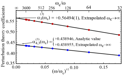
Figure 8: (Color online.) Plot of numerical approximations to the sums which give the coefficients $\alpha_{3}^{(3)}$ (red circles) and $\alpha_{4,3}^{(3)}$ (blue circles), with a hard cutoff $\omega_{c}$ in the energy of the intermediate states. The data is plotted versus $(\omega/\omega_{c})^{1/2}$ on the bottom axis (the top axis shows the corresponding value of $\omega_{c}/\omega$). The black lines are the least-square fits to the expected asymptotic behavior $a+b(\omega/\omega_{c})^{1/2}+c(\omega/\omega_{c})$. The values for $\alpha_{3}^{(3)}$ and $a_{4,3}^{(3)}$ are obtained by extrapolating to the y-intercept ($\omega_{c}\rightarrow\infty$). To estimate the one-standard deviation uncertainty in $\alpha_{3}^{(3)},$ for which we do not have an analytic value, we use the difference between the extrapolated and analytic values of $\alpha_{4,3}^{(3)}$.

B.3 Four-body, third-order coefficients $\alpha_{4,1}^{(3)}$ and $\alpha_{4,2}^{(3)}$

The contributions and give the coefficients

$$\alpha_{4,1}^{(3)}=\sum\limits_{i\neq 0,j}\frac{K_{00;ij}K_{j0;00}K_{i0;00}}{\Delta\varepsilon_{ij}\Delta\varepsilon_{i0}}$$ (130)

and

$$\alpha_{4,2}^{(3)}=\sum\limits_{i\neq 0,j\neq 0}\frac{K_{00;0i}K_{i0;0j}K_{j0;00}}{\Delta\varepsilon_{i0}\Delta\varepsilon_{j0}},$$ (131)

respectively. Due to angular momentum conservation, only $i,j$ with $l=m=0$ contribute. Using Eqs. (116), (120), and (115), we obtain the numerical results

$$\alpha_{4,1}^{(3)}=\sum_{n_{1}\neq 0,n_{2}=0}\frac{K_{\text{s.p.}}(n_{1},0,0)K_{\text{s.p.}}(n_{2},0,0)K_{\text{s.p.}}(n_{1},n_{2},0)}{4n_{1}(n_{1}+n_{2})}=0.077465...$$ (132)

and

$$\alpha_{4,2}^{(3)}=\sum_{n_{1}\neq 0,n_{2}\neq 0}\frac{K_{\text{s.p.}}(n_{1},0,0)K_{\text{s.p.}}(n_{1},n_{2},0)K_{\text{s.p.}}(n_{2},0,0)}{4n_{1}n_{2}}=0.051099....$$ (133)

These are tree-diagram processes, which, like $\alpha_{3}^{(2)},$ converge quickly, thereby making it is easy to obtain a precise numerical approximation from a small number of excited orbitals.

B.4 Four-body, third-order coefficient $\alpha_{4,3}^{(3)}$

The two-, three-, and four-body contributions $\raisebox{-3.61371pt}{\includegraphics{alpha3small}},\raisebox{-3.61371pt}{\includegraphics{beta3small}},$ and have the same coefficient,

$$\alpha_{4,3}^{(3)}=\sum\limits_{ij\neq 00}\frac{K_{00;ij}K_{00;00}K_{ij;00}}{\Delta\varepsilon_{ij}^{2}}=\sum\limits_{\tilde{\imath}\tilde{j}\neq 00}\frac{K_{00;\tilde{\imath}\tilde{j}}K_{00;00}K_{\tilde{\imath}\tilde{j};00}}{\Delta\varepsilon_{\tilde{\imath}\tilde{j}}^{2}},$$ (134)

where in the last expression, rather than evaluating the sums in the single-particle basis, we observe that $\phi_{000}(\mathbf{r}_{1})\phi_{000}(\mathbf{r}_{2})=\tilde{\phi}_{000}(\mathbf{r)}\tilde{\Phi}_{000}(\mathbf{R)}$ and sum over relative and center-of-mass bases states $|\tilde{\imath}\tilde{j}\rangle=|nlm,NLM\rangle,$ excluding $\tilde{\imath}\tilde{j}=00$. The interactions conserve the center-of-mass motion, implying $\tilde{j}=\{NLM\}=\{000\}$. Angular momentum conservation gives $\tilde{\imath}=\{n00\}$. Finally, using $\Delta\varepsilon_{n00,000}=2n$ and $K_{\tilde{\imath}0;00}=K_{n00,000;000,000}=K_{\text{rel}}(n,0)$ from Eq. (124), we obtain the analytic result

$$\alpha_{4,3}^{(3)} =\sqrt{\frac{2}{\pi}}\sum_{n>0}\frac{[K_{\text{rel}}(n,0)]^{2}}{4n^{2}}$$ (135)

$$=\left(\frac{2}{\pi}\right)^{3/2}[\frac{\pi^{2}}{24}+\log 2-\frac{1}{2}\left(\log 2\right)^{2}]=0.43894....$$

If we include the exponential regulator, we confirm that $\alpha_{4,3}^{(3)}\$converges as $\ (\omega/\omega_{c})^{1/2}$. Because the sums for $\alpha_{4,3}^{(3)}$ and $\alpha_{3}^{(3)}$ have the same asymptotic behaviors, we use the exact result in Eq. (135) to determine the accuracy of the extrapolation for $\alpha_{3}^{(3)}$ shown in Fig. 8.

B.5 Five-body, third-order coefficient $\alpha_{5}^{(3)}$

The three-, four-, and five-body contributions $\raisebox{-7.74022pt}{\includegraphics{beta4small}},\raisebox{-3.61371pt}{\includegraphics{gamma4small}},$ and have the same coefficient

$$\alpha_{5}^{(3)}=\sum\limits_{i\neq 0}\frac{K_{00;0i}K_{00;00}K_{i0;00}}{\Delta\varepsilon_{i0}{}^{2}}.$$ (136)

Working in the single-particle basis $|n_{1}l_{1}m_{1},n_{2}l_{2}m_{2}\rangle,$ we obtain the analytic result

$$\alpha_{5}^{(3)} =\sqrt{\frac{2}{\pi}}\sum_{n>0}\frac{[K_{\text{s.p.}}(n,0)]^{2}}{4n^{2}}$$

$$=\frac{3}{4(2\pi)^{3/2}}{}_{4}F_{3}(1,1,1,5/2;2,2,2;1/4)$$

$$=\left(\frac{2}{\pi}\right)^{3/2}[\frac{1}{2}\text{Li}_{2}(1/2-\sqrt{3}/4)-\log(1+\sqrt{3}/2)$$

$$\hskip 14.22636pt-\frac{1}{4}(\log(1+\sqrt{3}/2)-\log 2)^{2}+\log 2]$$

$$=0.051916...,$$ (137)

where ${}_{p}F_{q}$ is a generalized hypergeometric function, and Li${}_{2}(z)$ is the polylogarithm function. Evaluation with a regulator function shows that this expression converges as $(\omega/\omega_{c})^{1/2}$.

B.6 Two-body, second-order coefficient $\beta_{2}^{(2)}$

The coefficients $\beta_{m}^{(n)}(\omega)$ diverge when $\omega_{c}/\omega\rightarrow\infty$. The two-body contribution has the coefficient

$$\beta_{2}^{(2)}\left(\omega\right)=\sum\limits_{ij\neq 00}^{\omega_{c}/\omega}\frac{K_{00;ij}K_{ij;00}}{\Delta\varepsilon_{ij}}=\sum\limits_{\tilde{\imath}\neq 0}^{\omega_{c}/\omega}\frac{K_{00;\tilde{\imath}0}K_{\tilde{\imath}0;00}}{\Delta\varepsilon_{\tilde{\imath}0}},$$ (138)

where we have switched to the relative and center-of-mass basis $|\tilde{\imath}\tilde{j}\rangle=|nlm,NLM\rangle$ in the last expression. Using the fact that only $l=m=0$ and $\tilde{j}=0$ states contribute greatly simplifies the evaluation of $\beta_{2}^{(2)}(\omega)$ by reducing the multidimensional sum to a single summation. Using $K_{n00,000;000,000}=K_{\text{rel}}(n,0)$ from Eq. (124) and the exponential regulator $1/\Delta\varepsilon_{\tilde{\imath}0}\rightarrow e^{-2n(\omega/\omega_{c})}/2n,$ we obtain

$$\beta_{2}^{(2)}\left(\omega\right)=\sum\limits_{n>0}\frac{[K_{\text{rel}}(n,0)]^{2}}{2n}e^{-\frac{2n\omega}{\omega_{c}}}$$ (139)

$$=\left(\frac{2}{\pi}\right)\left(\sqrt{\frac{\omega_{c}}{2\omega}}-(1-\log 2)-\frac{3}{2}\sqrt{\frac{\omega}{2\omega_{c}}}\right)+\mathcal{O(}1/\omega_{c}).$$

This coefficient diverges as $\sqrt{\omega_{c}/\omega},$ but as shown in the main body of this paper, the divergence cancels after renormalization, leaving a finite correction proportional to $(2/\pi)(1-\log 2).$

B.7 Two-body, third-order coefficient $\beta_{2}^{(3)}$

Next we consider the contribution $\raisebox{-3.61371pt}{\includegraphics{alpha2small}},$ with coefficient

$$\beta_{2}^{(3)}\left(\omega\right)=\sum\limits_{ij\neq 00,kl\neq 00}\frac{K_{00;ij}K_{ij;kl}K_{kl;00}}{\Delta\varepsilon_{ij}\Delta\varepsilon_{kl}}=\sum\limits_{\tilde{\imath}\neq 0,\tilde{k}\neq 0}\frac{K_{00;\tilde{\imath}0}K_{\tilde{\imath}0;\tilde{k}0}K_{\tilde{k}0;00}}{\Delta\varepsilon_{\tilde{\imath}0}\Delta\varepsilon_{\tilde{k}0}},$$ (140)

where we again switch to relative and center-of-mass basis states and use the selection rules. Inserting exponential regulators for both energy denominators in Eq. (140) and using Eq. (123), it follows that

$$\beta_{2}^{(3)}(\omega) =\sum_{n>0,n^{\prime}>0}\frac{K_{\text{rel}}(n,0)K_{\text{rel}}(n,n^{\prime})K_{\text{rel}}(n^{\prime},0)}{4nn^{\prime}}e^{-\frac{2(n^{\prime}+n)\omega}{\omega_{c}}}$$

$$=\sqrt{\frac{\pi}{2}}\left(\sum_{n>0}\frac{[K_{\text{rel}}(n,0)]^{2}}{2n}e^{-\frac{2n\omega}{\omega_{c}}}\right)\left(\sum_{n^{\prime}>0}\frac{[K_{\text{rel}}(n^{\prime},0)]^{2}}{2n^{\prime}}e^{-\frac{2n^{\prime}\omega}{\omega}}\right)=[\beta_{2}^{(2)}\left(\omega\right)]^{2}/\alpha_{2}^{(1)}.$$ (141)

This factorization result is important for the renormalization of the two-body interaction at third- and higher-orders.

B.8 Three-body, third-order coefficient $\beta_{3}^{(3)}(\omega)$

The contribution gives the coefficient

$$\beta_{3}^{(3)}\left(\omega\right) =\sum\limits_{ij\neq 00,k\neq 0}\frac{K_{00;ij}K_{ij;0k}K_{k0;00}}{\Delta\varepsilon_{ij}\Delta\varepsilon_{k}}$$

$$=\sum\limits_{\tilde{\imath}\neq 0,k\neq 0}\frac{K_{00;\tilde{\imath}0}K_{\tilde{\imath}0;0k}K_{k0;00}}{\Delta\varepsilon_{\tilde{\imath}0}\Delta\varepsilon_{k0}}.$$ (142)

In the last equality, we replaced the sum over single-particle intermediate states $|ij\rangle$ with a sum over relative and center-of-mass states $|\tilde{\imath}\tilde{j}\rangle,$ and then used the selection rule $\tilde{j}=0.$ The sum over $k$ remains over the single-particle basis. We therefore require the “mixed-basis” matrix elements $K_{\tilde{\imath}0;0k}.$ Using the selection rules $l=m=0$ for the relative motion, and $l_{1}=m_{1}=0$ for the single-particle motion, we need only $K_{\tilde{\imath}0;0k}=K_{\text{mixed}}(n,n_{1})$ with $\tilde{\imath}=\{n00\}$ and $k=\{n_{1}00\},$ where

$$K_{\text{mixed}}(n,n_{1}) =\sqrt{\frac{2}{\pi}}(2\pi)^{3/2}\int\tilde{\phi}_{n00}^{\ast}\left(\mathbf{r}\right)\tilde{\phi}_{000}^{\ast}(\mathbf{R})\delta^{(3)}(\mathbf{r)}\phi_{n_{1}00}(\mathbf{r}_{1})\phi_{000}(\mathbf{r}_{2})d\mathbf{r}d\mathbf{R}$$

$$=\sqrt{\frac{2}{\pi}}(2\pi)^{3/2}\tilde{\phi}_{n00}\left(\mathbf{0}\right)\int\tilde{\phi}_{000}^{\ast}(\mathbf{R})\phi_{n_{1}00}(\frac{\mathbf{R}}{\sqrt{2}})\phi_{000}(\frac{\mathbf{R}}{\sqrt{2}})d\mathbf{R,}$$ (143)

and $\mathbf{r}_{1,2}=(\mathbf{R}\pm\mathbf{r)/}\sqrt{2}$. Substituting in harmonic oscillator wavefunctions gives

$$K_{\text{mixed}}(n,n_{1})=16\sqrt{2}\tilde{\phi}_{n00}\left(\mathbf{0}\right)N_{n_{1}0}\int_{0}^{\infty}L_{n_{1}}^{(1/2)}\left(x^{2}\right)e^{-2x^{2}}x^{2}dx,$$ (144)

where $x=\left|\mathbf{R}\right|/\sqrt{2}$ and we have integrated over the angles. Noting that the remaining integral over $x$ is proportional to $K_{\text{s.p.}}(n_{1},0,0)$ in Eq. (117), we find that

$$K_{\text{mixed}}(n,n_{1})=\sqrt{\frac{\pi}{2}}K_{\text{rel}}(n,0)K_{\text{s.p.}}(n_{1},0,0).$$ (145)

Inserting exponential regulators for each energy denominator in Eq. (142), we obtain

$$\beta_{3}^{(3)}(\omega) =\sum_{n>0,n_{1}>0}\frac{K_{\text{rel}}(n,0)K_{\text{mixed}}(n,n_{1})K_{\text{s.p.}}(n_{1},0,0)}{4nn_{1}}e^{-\frac{2(n+n_{1})\omega}{\omega_{c}}}$$

$$=\sqrt{\frac{\pi}{2}}\left(\sum_{n_{1}>0}\frac{[K_{\text{s.p.}}(n_{1},0,0)]^{2}}{2n_{1}}e^{-\frac{2n_{1}\omega}{\omega_{c}}}\right)\left(\sum_{n>0}\frac{[K_{\text{rel}}(n,0)]^{2}}{2n}e^{-\frac{2n\omega}{\omega_{c}}}\right)=\alpha_{3}^{(2)}\beta_{2}^{(2)}(\omega)/\alpha_{2}^{(1)}.$$ (146)

The factorization of $\beta_{3}^{(3)}$ in the finite part $\alpha_{3}^{(2)}/\alpha_{2}^{(1)}$ and the divergent part $\beta_{2}^{(2)}(\omega)$ is important for the renormalization of the three-body interaction at third order.

References

- Bloch et al. (2008) I. Bloch, J. Dalibard, and W. Zwerger, Rev. Mod. Phys. 80, 885 (2008).
- Chin et al. (2010) C. Chin, R. Grimm, P. Julienne, and E. Tiesinga, Rev. Mod. Phys. 82, 1225 (2010).
- Efimov (1970) V. Efimov, Phys. Lett. B 33, 563 (1970).
- Nielsen and Macek (1999) E. Nielsen and J. H. Macek, Phys. Rev. Lett. 83, 1566 (1999).
- Esry et al. (1999) B. D. Esry, C. H. Greene, and J. P. Burke, Phys. Rev. Lett. 83, 1751 (1999).
- Bedaque et al. (2000) P. F. Bedaque, E. Braaten, and H.-W. Hammer, Phys. Rev. Lett. 85, 908 (2000).
- Kraemer et al. (2006) T. Kraemer, M. Mark, P. Waldburger, J. Danzl, C. Chin, B. Engeser, A. Lange, K. Pilch, A. Jaakkola, H.-C. Nägerl, et al., Nature 85, 315 (2006).
- Braaten and Hammer (2007) E. Braaten and H.-W. Hammer, Ann. Phys. 322, 120 (2007).
- Braaten and Hammer (2006) E. Braaten and H.-W. Hammer, Phys. Rep. 428, 259 (2006).
- Torrontegui et al. (2011) E. Torrontegui, A. Ruschhaupt, D. Guéry-Odelin, and J. G. Muga, Journal of Physics B: Atomic, Molecular and Optical Physics 44, 195302 (2011).
- Beane et al. (2007) S. R. Beane, W. Detmold, and M. J. Savage, Phys. Rev. D 76, 074507 (2007).
- Maeda et al. (2009) K. Maeda, G. Baym, and T. Hatsuda, Phys. Rev. Lett. 103, 085301 (2009).
- Hammer and Platter (2007) H. Hammer and L. Platter, The European Physical Journal A - Hadrons and Nuclei 32, 113 (2007).
- von Stecher et al. (2009) J. von Stecher, J. P. D’Incao, and C. H. Greene, Nature Physics 5, 417 (2009).
- Pollack et al. (2009) S. E. Pollack, D. Dries, and R. G. Hulet, Science 326, 1683 (2009).
- Ferlaino et al. (2009) F. Ferlaino, S. Knoop, M. Berninger, W. Harm, J. P. D’Incao, H.-C. Nägerl, and R. Grimm, Phys. Rev. Lett. 102, 140401 (2009).
- Will et al. (2010) S. Will, T. Best, U. Schneider, L. Hackermüller, D. Lühmann, and I. Bloch, Nature 465, 197 (2010).
- Johnson et al. (2009) P. R. Johnson, E. Tiesinga, J. V. Porto, and C. J. Williams, New J. Phys. 11, 093022 (2009).
- Tiesinga and Johnson (2011) E. Tiesinga and P. R. Johnson, Phys. Rev. A 83, 063609 (2011).
- Greiner et al. (2002) M. Greiner, O. Mandel, T. W. Hänsch, and I. Bloch, Nature 419, 51 (2002).
- Anderlini et al. (2006) M. Anderlini, J. Sebby-Strabley, J. Kruse, J. V. Porto, and W. D. Phillips, J. Phys. B 39, S199 (2006).
- Sebby-Strabley et al. (2007) J. Sebby-Strabley, B. L. Brown, M. Anderlini, P. J. Lee, W. D. Phillips, J. V. Porto, and P. R. Johnson, Phys. Rev. Lett. 98, 200405 (2007).
- Ma et al. (2011) R. Ma, M. E. Tai, P. M. Preiss, W. S. Bakr, J. Simon, and M. Greiner, Phys. Rev. Lett. 107, 095301 (2011).
- Mark et al. (2011) M. J. Mark, E. Haller, K. Lauber, J. G. Danzl, A. J. Daley, and H.-C. Nägerl, Phys. Rev. Lett. 107, 175301 (2011).
- Büchler et al. (2007) H. Büchler, A. Micheli, and P. Zoller, Nature Physics 3, 726 (2007).
- Chen et al. (2008) B.-l. Chen, X.-b. Huang, S.-p. Kou, and Y. Zhang, Phys. Rev. A 78, 043603 (2008).
- Schmidt et al. (2008) K. P. Schmidt, J. Dorier, and A. Läuchli, Phys. Rev. Lett. 101, 150405 (2008).
- Capogrosso-Sansone et al. (2009) B. Capogrosso-Sansone, S. Wessel, H. P. Büchler, P. Zoller, and G. Pupillo, Phys. Rev. B 79, 020503(R) (2009).
- Mazza et al. (2010) L. Mazza, M. Rizzi, M. Lewenstein, and J. I. Cirac, Phys. Rev. A 82, 043629 (2010).
- Zhou et al. (2010) K. Zhou, Z. Liang, and Z. Zhang, Phys. Rev. A 82, 013634 (2010).
- Will et al. (2011) S. Will, T. Best, S. Braun, U. Schneider, and I. Bloch, Phys. Rev. Lett. 106, 115305 (2011).
- Singh et al. (2012) M. Singh, A. Dhar, T. Mishra, R. V. Pai, and B. P. Das, ArXiv e-prints (2012), eprint 1203.1412.
- Srednicki (2007) M. Srednicki, Quantum Field Theory (Cambridge University Press, 2007).
- Busch et al. (1998) T. Busch, B.-G. Englert, K. Rza̧żewski, and M. Wilkens, Found. of Phys. 28, 549 (1998).
- Fisher et al. (1989) M. P. A. Fisher, P. B. Weichman, G. Grinstein, and D. S. Fisher, Phys. Rev. B 40, 546 (1989).
- Jaksch et al. (1998) D. Jaksch, C. Bruder, J. I. Cirac, C. W. Gardiner, and P. Zoller, Phys. Rev. Lett. 81, 3108 (1998).
- Mering and Fleischhauer (2011) A. Mering and M. Fleischhauer, Phys. Rev. A 83, 063630 (2011).
- Schachenmayer et al. (2011) J. Schachenmayer, A. J. Daley, and P. Zoller, Phys. Rev. A 83, 043614 (2011).
- Buchhold et al. (2011) M. Buchhold, U. Bissbort, S. Will, and W. Hofstetter, Phys. Rev. A 84, 023631 (2011).
- Rigol et al. (2006) M. Rigol, A. Muramatsu, and M. Olshanii, Phys. Rev. A 74, 053616 (2006).
- Fischer and Schützhold (2008) U. R. Fischer and R. Schützhold, Phys. Rev. A 78, 061603 (2008).
- Wolf et al. (2010) F. A. Wolf, I. Hen, and M. Rigol, Phys. Rev. A 82, 043601 (2010).
- Ananikian and Bergeman (2006) D. Ananikian and T. Bergeman, Phys. Rev. A 73, 013604 (2006).
- Fölling et al. (2007) S. Fölling, S. Trotsky, P. Cheinet, N. Feld, R. Saers, A. Widera, T. Müller, and I. Bloch, Nature 448, 1029 (2007).
- Zhou et al. (2011) Q. Zhou, J. V. Porto, and S. Das Sarma, Phys. Rev. A 84, 031607 (2011).
- Pielawa et al. (2011) S. Pielawa, T. Kitagawa, E. Berg, and S. Sachdev, Phys. Rev. B 83, 205135 (2011).
- Alon et al. (2005) O. E. Alon, A. I. Streltsov, and L. S. Cederbaum, Phys. Rev. Lett. 95, 030405 (2005).
- Alon et al. (2007) O. E. Alon, A. I. Streltsov, and L. S. Cederbaum, Phys. Lett. A 362, 453 (2007).
- Hazzard and Mueller (2010) K. R. A. Hazzard and E. J. Mueller, Phys. Rev. A 81, 031602 (2010).
- Lühmann et al. (2012) D.-S. Lühmann, O. Jürgensen, and K. Sengstock, New Journal of Physics 14, 033021 (2012).
- Bissbort et al. (2011) U. Bissbort, F. Deuretzbacher, and W. Hofstetter, ArXiv e-prints (2011), eprint 1108.6047.
- Cao et al. (2011) L. Cao, I. Brouzos, S. Zöllner, and P. Schmelcher, New J. Phys. 13, 033032 (2011).
- Blume et al. (2007) D. Blume, J. von Stecher, and C. H. Greene, Phys. Rev. Lett. 99, 233201 (2007).
- Lühmann et al. (2008) D.-S. Lühmann, K. Bongs, K. Sengstock, and D. Pfannkuche, Phys. Rev. Lett. 101, 050402 (2008).
- Lutchyn et al. (2009) R. M. Lutchyn, S. Tewari, and S. Das Sarma, Phys. Rev. A 79, 011606 (2009).
- Rotureau et al. (2010) J. Rotureau, I. Stetcu, B. R. Barrett, M. C. Birse, and U. van Kolck, Phys. Rev. A 82, 032711 (2010).
- Burt et al. (1997) E. A. Burt, R. W. Ghrist, C. J. Myatt, M. J. Holland, E. A. Cornell, and C. E. Wieman, Phys. Rev. Lett. 79, 337 (1997).
- Fedichev et al. (1996) P. O. Fedichev, M. W. Reynolds, and G. V. Shlyapnikov, Phys. Rev. Lett. 77, 2921 (1996).
- Mazets and Schmiedmayer (2010) I. E. Mazets and J. Schmiedmayer, New J. Phys. 12, 055023 (2010).
- Taylor (2002) R. Taylor, Scattering Theory of Waves and Particles (Dover Publications, Inc., New York, 2002).
- Bolda et al. (2002) E. L. Bolda, E. Tiesinga, and P. S. Julienne, Phys. Rev. A 66, 013403 (2002).
- Blume and Greene (2002) D. Blume and C. H. Greene, Phys. Rev. A 65, 043613 (2002).
- von Stecher et al. (2008) J. von Stecher, C. H. Greene, and D. Blume, Phys. Rev. A 77, 043619 (2008).
- Suzuki and Varga (1998) Y. Suzuki and K. Varga, Stochastic Variational Approach to Quantum Mechanical Few-Body Problems (Springer Verlag, Berlin, 1998).
- Mott and Massey (1965) N. F. Mott and H. S. W. Massey, Theory of Atomic Collisions (Oxford University Press, London, 1965), 3rd ed.
- Gao (1998) B. Gao, Phys. Rev. A 58, 4222–4225 (1998).
- Huang and Yang (1957) K. Huang and C. N. Yang, Phys. Rev. 105, 767 (1957).
- Fetter and Walecka (1971) A. L. Fetter and J. D. Walecka, Quantum theory of Many-Particle Systems (McGraw-Hill, 1971).
- Talman (1970) J. D. Talman, Nucl. Phys. A 141, 273 (1970).
- Edwards et al. (1996) M. Edwards, R. Dodd, C. Clark, and K. Burnett, J. Res. Natl. Inst. Stand. Technol. 101, 553 (1996).
- DLM (2011) Digital Library of Mathematical Functions. Release date 2011-08-29. (National Institute of Standards and Technology from http://dlmf.nist.gov/18.10.E8, 2011).