Likelihood-ratio ranking of gravitational-wave candidates in a non-Gaussian background.

Abstract

We describe a general approach to detection of transient gravitational-wave signals in the presence of non-Gaussian background noise. We prove that under quite general conditions, the ratio of the likelihood of observed data to contain a signal to the likelihood of it being a noise fluctuation provides optimal ranking for the candidate events found in an experiment. The likelihood-ratio ranking allows us to combine different kinds of data into a single analysis. We apply the general framework to the problem of unifying the results of independent experiments and the problem of accounting for non-Gaussian artifacts in the searches for gravitational waves from compact binary coalescence in LIGO data. We show analytically and confirm through simulations that in both cases the likelihood ratio statistic results in an improved analysis.

I Introduction

The detection of gravitational waves from astrophysical sources is a long-standing problem in physics. Over the past decade, the experimental emphasis has been on the construction and operation of kilometer-scale interferometric detectors such as Laser Interferometer Gravitational-wave Observatory (LIGO) Abbott et al. (2009). The instruments measure the strain, $s(t)$, by monitoring light at the interferometer’s output port, which varies as test masses that are suspended in vacuum at the ends of orthogonal arms differentially approach and recede by minuscule amounts. The strain signal, $s(t)$, is a combination of noise, $n(t)$, and gravitational-wave signal, $h(t)$.

There is a well established literature describing the analysis of time-series data for signals of various types Wainstein and Zubakov (1962); these methods have been extended to address gravitational-wave detection Finn and Chernoff (1993). This approach usually begins with the assumption that the detector noise, $n(t)$, is stationary and Gaussian. Then one proceeds to derive a set of filters that are tuned to detect the particular signals in this time-series data. The result is both elegant and powerful: whitened detector noise is correlated with a whitened version of the expected signal. The approach has been used to develop techniques to search for gravitational waves from compact binary coalescence, isolated neutron stars, stochastic sources, and generic bursts with certain time-frequency characteristics Anderson et al. (2001).

This approach takes the important first step of designing filters that properly suppress the dominant, frequency-dependent noise sources in the instrument. The simplicity of the filters is due to the fact that the power-spectral density fully characterizes the statistical properties of stationary, Gaussian noise. However, interferometric detectors are prone to non-Gaussian and non-stationary noise sources. Environmental disturbances, including seismic, acoustic, and electromagnetic effects, can lead to artifacts in the time series that are neither gravitational waves nor stationary, Gaussian noise. Imperfections in hardware can lead to unwanted signals in the time series that originate from auxiliary control systems.

To help identify and remove these unwanted signals, instruments have been constructed at geographically separated sites and the data are analyzed together. A plethora of diagnostics have also been developed to characterize the quality of the data Christensen (2010) (for the LIGO Scientific Collaboration and the Virgo Collaboration); Robinet (2010) (for the LIGO Scientific Collaboration and the Virgo Collaboration); Macleod et al. (2011). Searches for gravitational waves use more than just the filtered output of the time-series, $s(t)$, to separate gravitational-wave signals from noise. Moreover, the responses from various filters indicate that the underlying noise sources are not Gaussian, even after substantial data quality filtering and coincidence requirements have been applied.

In this paper, we discuss using likelihood-ratio ranking as a unified approach to gravitational-wave data analysis. The approach foregoes the stationary, Gaussian model of the detector noise. The output of the filters derived under that assumption becomes one element in a list of parameters that characterize a gravitational-wave detection candidate. The detection problem is then couched in terms of the statistical properties of an $n$-tuple of derived quantities, leading directly to a likelihood-ratio ranking for detection candidates. The $n$-tuple can include more information than simply the signal-to-noise ratio (SNR) measured in each instrument of the network. It can include measures of data quality, the physical parameters of the gravitational-wave candidate, the SNR from the coherent and null combinations of the detector signals; it can include nearly any measure of detector behavior or signal quality.

This approach was already used to develop ranking statistics for compact binary coalescence signals Abbott et al. (2008); Abadie et al. (2010, 2010) and is at the core of a powerful coincidence test developed for burst searches Cannon (2008).

This work presents a general framework for the likelihood-ratio ranking in the context of gravitational-wave detection. We explore its analytical properties and illustrate its practical value by applying it to two data analysis problems arising in real-life searches for gravitational waves in LIGO data.

II General derivation of likelihood-ratio ranking

Let the $n$-tuple $\vec{c}$ denote the observable data in some experiment that aims to detect a signal denoted by $\mathbf{h}$. This signal can usually be parametrized by several continuous parameters that may be unknown, for example distance to the source of gravitational waves and location on the sky. The purpose of the experiment is to identify the signal. Depending on whether a Bayesian or frequentist statistical approach is taken, this is stated in terms of either the probability that the signal is present or the probability that the observed data are a noise fluctuation.

In this section, we show that both approaches lead to ranking candidate signals according to the likelihood ratio

$$\Lambda(\vec{c})=\frac{\int\!p(\vec{c}\,|\,\mathbf{h},1)p(\mathbf{h}\,|\,1)\,\mathrm{d}\mathbf{h}}{p(\vec{c}\,|\,0)}\,,$$ (1)

where $p(\vec{c}\,|\,\mathbf{h},1)$ is the probability of observing $\vec{c}$ in the presence of the signal $\mathbf{h}$, $p(\mathbf{h}\,|\,1)$ is the prior probability to receive that signal, and $p(\vec{c}\,|\,0)$ is the probability of observing $\vec{c}$ in the absence of any signal. The higher a candidate’s $\Lambda$ value, the more likely it is a real signal.

II.1 Bayesian Analysis

In this approach, we compute the probability that a signal is present in the observed data, $p(1\,|\,\vec{c})$. By a straightforward application of Bayes theorem, we write

$$p(1\,|\,\vec{c}) =\frac{p(\vec{c}\,|\,1)p(1)}{p(\vec{c}\,|\,1)p(1)+p(\vec{c}\,|\,0)p(0)}$$

$$=\frac{\int\!p(\vec{c}\,|\,\mathbf{h},1)p(\mathbf{h}\,|\,1)p(1)\,\mathrm{d}\mathbf{h}}{\int\!p(\vec{c}\,|\,\mathbf{h},1)p(\mathbf{h}\,|\,1)p(1)\,\mathrm{d}\mathbf{h}+p(\vec{c}\,|\,0)p(0)}\,,$$ (2)

where $p(0)$ is the a priori probability that the signal is absent and $p(1)$ is the a priori probability that there is a signal (of any kind). The denominator re-expresses $p(\vec{c})$ in terms of the two possible independent outcomes: the signal is present or the signal is absent. Upon successive division of numerator and denominator by $p(\vec{c}\,|\,0)$ and $p(1)$, we find

$$p(1\,|\,\vec{c})=\frac{\Lambda(\vec{c})}{\Lambda(\vec{c})+p(0)/p(1)}\,,$$ (3)

which is a monotonically increasing function of the likelihood ratio $\Lambda$ defined by Eq. (1) . Hence, the larger the likelihood ratio, the more probable it is that a signal is present.

II.2 Frequentist Approach

The process of detection can always be reduced to a binary “yes” or “no” question—does the observed data contain the signal? An optimal detection scheme should achieve the maximum rate of successful detections—correctly given “yes” answers—with some fixed, preferably low, rate of false alarms or false positives—incorrectly given “yes” answers. This is the essence of the Neyman-Pearson optimality criteria for detection, which states that an optimal detector should maximize the probability of detection at a fixed probability of false alarm Neyman and Pearson (1933).

As before, let the $n$-tuple $\vec{c}$ denote the observable data and $\mathbf{h}$ the signal that is the object of the search. Without loss of generality, any decision-making algorithm can be mapped into a real function, $f(\vec{c})$, of the data that signifies detection whenever its value is greater than or equal to a threshold value, $F^{\ast}$. Thus, using the Neyman-Pearson formalism, an optimal detector is realized by finding a function, $f(\vec{c})$, that maximizes the probability of detection at a fixed value of the probability of false alarm. The probability of detection, $P_{1}$, is

$$P_{1}=\int_{V_{d}}\int_{V_{\mathbf{h}}}\!\Theta\left(f(\vec{c})-F^{\ast}\right)p(\vec{c}\,|\,\mathbf{h},1)p(\mathbf{h}\,|\,1)p(1)\,\mathrm{d}\mathbf{h}\,\mathrm{d}\vec{c}\,,$$ (4)

and the probability of false alarm , $P_{0}$, is

$$P_{0}=\int_{V_{\mathrm{d}}}\!\Theta\left(f(\vec{c})-F^{\ast}\right)p(\vec{c}\,|\,0)p(0)\,\mathrm{d}\vec{c}\,,$$ (5)

where $V_{\mathbf{h}}$ identifies the subset of signals targeted by the search, $V_{\mathrm{d}}$ denotes the subset of accessible data and integration is performed over all signals, $\mathbf{h}$, and data points, $\vec{c}$, within these subsets. Treating $P_{1}$ and $P_{0}$ as functionals of $f(\vec{c})$, we find that for an optimal detector, the variation of

$$S[f(\vec{c})]=P_{1}[f(\vec{c})]-l_{0}\left(P_{0}[f(\vec{c})]-P^{\ast}\right)$$ (6)

should vanish. Here $l_{0}$ denotes a Lagrange multiplier and $P^{\ast}$is a constant that sets the value of the probability of false alarm. The variation of Eq. (6) with respect to $f(\vec{c})$ gives

$$\delta S= \int_{V_{\mathrm{d}}}\!\delta\left(f(\vec{c})-F^{\ast}\right)\delta f(\vec{c})$$

$$\times\left[\int_{V_{\mathbf{h}}}p(\vec{c}\,|\,\mathbf{h},1)p(\mathbf{h}\,|\,1)p(1)\,\mathrm{d}\mathbf{h}-l_{0}p(\vec{c}\,|\,0)p(0)\right]\,\mathrm{d}\vec{c}\,.$$ (7)

Variations $\delta f(\vec{c})$ at different data points are independent, thus implying that after integration over $\vec{c}$, the condition

$$\frac{\int\!p(\vec{c^{\ast}}\,|\,\mathbf{h},1)p(\mathbf{h}\,|\,1)\,\mathrm{d}\mathbf{h}}{p(\vec{c^{\ast}}\,|\,0)}=\frac{l_{0}p(0)}{p(1)}=\text{const}$$ (8)

must be satisfied at all points $\vec{c^{\ast}}$ for which the argument of the delta function satisfies the condition

$$f(\vec{c^{\ast}})-F^{\ast}=0\,.$$ (9)

This latter condition defines the detection surface separating the detection and non-detection regions. Note that as $f(\vec{c})$ varies, the shape of this surface changes accordingly. Therefore, Eq. (8) implies that the detection surface must be the surface of the constant likelihood ratio for an optimal detector. This is the only condition on the functional form of $f(\vec{c})$. Variation with respect to $F^{\ast}$ does not give a new condition, whereas variation with respect to the Lagrange multiplier, $l_{0}$, simply sets the probability of a false alarm to be $P^{\ast}$. 

A natural way to satisfy the optimality criteria is to use the likelihood ratio

$$\Lambda(\vec{c})=\frac{\int\!p(\vec{c}\,|\,\mathbf{h},1)p(\mathbf{h}\,|\,1)\,\mathrm{d}\mathbf{h}}{p(\vec{c}\,|\,0)}$$ (10)

or any function $f(\Lambda(\vec{c}))$ for ranking the candidate signals. With this choice, the optimality condition Eq. (8) is satisfied for any threshold $F^{\ast}$. The latter is determined by the choice of an admissible value of the probability of false alarm, $P^{\ast}$, through

$$P_{0}[f(\Lambda(\vec{c}))]=P^{\ast}\,.$$ (11)

II.3 Variation of efficiency with volume of search space

The likelihood ratio given in Eq. (1) is guaranteed to maximize the probability of signal detection for a given search. Because optimization is performed for a fixed region defined by all possible values of a candidate’s parameters, $\vec{c}$, in the search, it is unclear whether increasing the volume of available data (e.g. extension of the bank of template waveforms) would not result in an overall decrease of probability to detect signals. For example, one may be apprehensive of the potential increase in the rate of false alarms solely due to extension of the parameter space. Intuitively, having more available information should not negatively affect the detection probability or efficiency if the information is processed correctly. In what follows, we prove that this is true if the likelihood ratio is used for making the detection decision.

To prove that the detection efficiency does not decrease when the volume of data is increased, we must show that the variation of $\delta P_{1}/\delta V_{\mathrm{d}}$ at a fixed $P_{0}$ is non-negative. Consider a foliation of the space of data, $V_{\mathrm{d}}$, by surfaces of constant likelihood ratio, $S_{\Lambda}$. Functionals for the probabilities of detection, Eq. (4), and false alarm, Eq. (5) can be written as

$$P_{1}=\int_{0}^{\infty}\!\,\mathrm{d}\Lambda\int_{S_{\Lambda}}\!\Theta\left(\Lambda-\Lambda^{*}\right)p(\vec{c}\,|\,1)p(1)\,,$$ (12)

and

$$P_{0}=\int_{0}^{\infty}\!\,\mathrm{d}\Lambda\int_{S_{\Lambda}}\!\Theta\left(\Lambda-\Lambda^{*}\right)p(\vec{c}\,|\,0)p(0)\,,$$ (13)

where, for brevity, we absorbed explicit integration in the space of signals, $V_{\mathbf{h}}$, in the product $p(\vec{c}\,|\,1)p(1)$. $P_{1}$ is a functional of $V_{\mathrm{d}}$ and $\Lambda^{*}$. Since the latter is determined by the value chosen for false alarm probability, $P_{0}=P^{*}$, and the probability of false alarm also depends on $V_{\mathrm{d}}$, variations of $V_{\mathrm{d}}$ and $\Lambda^{*}$ are not independent. To find the relation, we vary the probability of false alarm

$$\begin{split}\delta P_{0}=&-\int_{0}^{\infty}\!\,\mathrm{d}\Lambda\int_{S_{\Lambda}}\!\delta\left(\Lambda-\Lambda^{*}\right)p(\vec{c}\,|\,0)p(0)\delta\Lambda^{*}\\ &+\int_{0}^{\infty}\!\,\mathrm{d}\Lambda\int_{\delta S_{\Lambda}}\!\Theta\left(\Lambda-\Lambda^{*}\right)p(\vec{c}\,|\,0)p(0)\delta S_{\Lambda}\,.\end{split}$$ (14)

We consider non-negative variations of surfaces of constant likelihood ratio, $\delta S_{\Lambda}$, that correspond only to the addition of new data points to $V_{\mathrm{d}}$, and therefore correspond only to an extension of surfaces, $S_{\Lambda}$, without an overall translation or change of shape.

The probability of false alarm should stay constant, therefore its variation should vanish, providing the relation

$$\delta\Lambda^{*}=\frac{\int_{0}^{\infty}\!\,\mathrm{d}\Lambda\int_{\delta S_{\Lambda}}\!\Theta\left(\Lambda-\Lambda^{*}\right)p(\vec{c}\,|\,0)\delta S_{\Lambda}}{\int_{S_{\Lambda^{*}}}\!p(\vec{c}\,|\,0)}\,.$$ (15)

Next, we vary the functional for the detection probability

$$\begin{split}\delta P_{1}=&-\Lambda^{*}\int_{S_{\Lambda^{*}}}\!p(\vec{c}\,|\,0)p(1)\delta\Lambda^{*}\\ &+\int_{0}^{\infty}\!\,\mathrm{d}\Lambda\int_{\delta S_{\Lambda}}\!\Theta\left(\Lambda-\Lambda^{*}\right)\Lambda\,p(\vec{c}\,|\,0)p(1)\delta S_{\Lambda}\,,\end{split}$$ (16)

where we use $p(\vec{c}\,|\,1)=\Lambda(\vec{c})p(\vec{c}\,|\,0)$, which follows from the definition of the likelihood ratio. Eliminating $\delta\Lambda^{*}$ by means of Eq. (15) and re-arranging terms we get

$$\delta P_{1}=p(1)\int_{0}^{\infty}\!\,\mathrm{d}\Lambda\int_{\delta S_{\Lambda}}\!\Theta\left(\Lambda-\Lambda^{*}\right)\left(\Lambda-\Lambda^{*}\right)p(\vec{c}\,|\,0)\delta S_{\Lambda}\,,$$ (17)

which is non-negative for all positive $\delta S_{\Lambda}$ by virtue of $\Theta\left(\Lambda-\Lambda^{*}\right)\left(\Lambda-\Lambda^{*}\right)\geq 0$. This proves that if the likelihood-ratio statistic is used in the detection process, the probability of detection can never decrease during an extension of the volume of available data.

III Applications

In Section III.1, we apply the formalism of Section II when assessing the significance of triggers between experiments on disjoint times. In Section III.2, we demonstrate how the likelihood-ratio ranking can improve analysis efficiency by accounting for non-Gaussian features in the distributions of parameters of the candidates events.

III.1 Combining disjoint experiments

One complexity that arises in real-world applications is the necessity to combine results from multiple independent experiments. For example, gravitational-wave searches are often thought of in terms of times when a fixed number of interferometers are operating. If a network consists of instruments that are not identical and located at different places, each combination of operating interferometers may have very different combined sensitivity and background noise. Times when three interferometers are recording data may be treated differently from those when any pair is operating. Ideally, these experiments would be treated together accounting for differences in detectors’ sensitivities and background noise in the ranking of the candidate signals, but it is often not practical (see how this problem was addressed in Abadie et al. (2010)). In this section, we show that the likelihood-ratio ranking offers a natural solution to this problem, which is conceptually similar to a simplified approach taken in Abadie et al. (2010).

Consider a situation in which the data is written as $\vec{c}=(\vec{d},j)$, where $j=0,1,2,\ldots$ indicates that the data arose from an experiment covering some time interval $T_{j}$. Note that $T_{i}\cap T_{j}=\emptyset$ if $j\neq i$. The probability that a signal is present given the data is

$$p(1\,|\,\vec{d},j)=\frac{\int\!p(\vec{d},j\,|\,\mathbf{h},1)p(\mathbf{h}\,|\,1)p(1)\,\mathrm{d}\mathbf{h}}{\int\!p(\vec{d},j\,|\,\mathbf{h},1)p(\mathbf{h}\,|\,1)p(1)\,\mathrm{d}\mathbf{h}+p(\vec{d},j\,|\,0)p(0)}\,.$$ (18)

The conditional probabilities for the observed data can be further expanded as

$$p(\vec{d},j\,|\,\mathbf{h},1) =p(\vec{d}\,|\,j,\mathbf{h},1)p(j\,|\,\mathbf{h},1)$$ (19)

$$p(\vec{d},j\,|\,0) =p(\vec{d}\,|\,j,0)p(j\,|\,0)\,,$$ (20)

where we introduce $p(j\,|\,\mathbf{h},1)$ and $p(j\,|\,0)$—the probabilities for the observed data to be from the $j^{\mathrm{th}}$ experiment given the presence or absence of a signal respectively. It is reasonable to assume that $p(j\,|\,\mathbf{h},1)=p(j\,|\,0)$. In this case, both probabilities drop out of Eq. (18), and the expression for the probability for a signal to be present in the data can be written as

$$p(1\,|\,\vec{d},j)=\frac{\Lambda(\vec{d},j)}{\Lambda(\vec{d},j)+p(0)/p(1)}\,,$$ (21)

with the likelihood ratio $\Lambda(\vec{d},j)$ given by

$$\Lambda(\vec{d},j)=\frac{\int\!p(\vec{d}\,|\,j,\mathbf{h},1)p(\mathbf{h})\,\mathrm{d}\mathbf{h}}{p(\vec{d}\,|\,j,0)}\,.$$ (22)

Comparing Eq. (21) with Eq. (3), we conclude that the likelihood ratio $\Lambda(\vec{d},j)$, evaluated independently for each experiment, provides optimal unified ranking. In terms of their likelihood ratios, data samples from different experiments can be compared directly, with differences in experiments’ sensitivities and noise levels being accounted for by $p(\vec{d}\,|\,j,\mathbf{h},1)$ and $p(\vec{d}\,|\,j,0)$.

Following the steps outlined in Section II.2, the same result can also be attained by direct optimization of the combined probability of detection at the fixed probability of false alarm. Optimality guarantees that the results of the less sensitive experiment can be combined with the results of the more sensitive experiment without loss of efficiency. In this approach, a unified scale provided by the likelihood ratio, $\Lambda(\vec{d},j)$, is explicit because, by construction, the same threshold, $F^{\ast}$, is applied to all data samples. $F^{\ast}$ is determined by the value of the probability of false alarm for the combined experiment, given by

$$P_{0}=\sum_{j}\int\!\Theta\left(\Lambda(\vec{d},j)-F^{\ast}\right)p(\vec{d}\,|\,j,0)p(j\,|\,0)p(0)\,\mathrm{d}\vec{d}\,,$$ (23)

which makes the whole process less trivial. Notice that $p(j\,|\,0)$ (often approximated by $T_{j}/\sum_{i}T_{i}$) appears in the expression for $P_{0}$, however it does not appear in the expression for the likelihood ratio given in Eq. (22). Since $p(j\,|\,0)$ is proportional to the experiment duration, $T_{j}$, each experiment is weighted appropriately in the total probability of false alarm. In a similar fashion, experiment durations appear in the expression for the combined efficiency or the probability of detection for the combined experiment.

III.2 Combining search spaces

Sophisticated searches for gravitational-wave signals from compact binary coalescence Abbott et al. (2008, 2009, 2009); Abadie et al. (2010) have been developed over the past decade. The non-Gaussian and non-stationary noise is substantially suppressed by the application of instrumental and environmental vetoes Christensen (2010) (for the LIGO Scientific Collaboration and the Virgo Collaboration); Robinet (2010) (for the LIGO Scientific Collaboration and the Virgo Collaboration); Macleod et al. (2011), coincidence between detectors, and numerous other checks on the quality of putative gravitational-wave signals. Nevertheless, the number of background triggers as a function of SNR depends on the masses of the binaries targeted in a search. For this reason, triggers have been divided into categories based on the chirp mass, $\mathcal{M}$, of the filters that produced the trigger (where $\mathcal{M}=((m_{1}m_{2})^{3}/(m_{1}+m_{2}))^{1/5}$ and $m_{1}$ and $m_{2}$ are the masses of the compact objects in the binary). The background is a slowly varying function of $\mathcal{M}$, falling off more rapidly, as a function of SNR, for smaller values of $\mathcal{M}$. This is a manifestation of non-Gaussianities still present in the data. It is desirable to account for this dependence when ranking candidates found in the search.

In this section, we consider a toy problem that mimics the properties of the compact binary search but demonstrates how the likelihood-ratio ranking matches our intuition. Following that example, we present the results of a simulated compact binary search and demonstrate that the detection statistic based on the likelihood ratio accounts for non-Gaussian features in background distribution and improves search efficiency.

III.2.1 Toy Problem

Consider an experiment in which the data that define a candidate are $\vec{c}=(\rho,x)$, where $\rho$ is the SNR and $x$ is the extra parameter describing the data sample (e.g. the chirp mass of the binary). Suppose the distribution of the data in the absence of a signal is

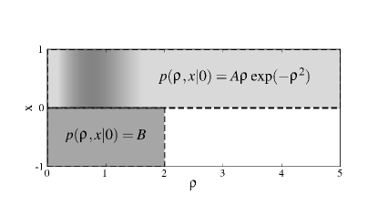
Figure 1: Graphic representation of the model background distribution of Eq. (24) for $\alpha=2.0$. Shaded areas define the regions of non-zero probability.

$$\begin{split}p(\rho,x\,|\,0)=&A\rho\exp(-\rho^{2})\Theta(x)\Theta(1-x)\\ &+B\Theta(x+1)\Theta(-x)\Theta(\rho)\Theta(\alpha-\rho)\,.\end{split}$$ (24)

Figure 1 provides a graphic representation of this distribution. Notice that $p(\rho,x\,|\,0)=0$ for $x<0$ and $\rho>\alpha$, therefore data $(\rho,x)$ in this region of the plane indicates the presence of a signal with unit probability. This intuition is clearly borne out in the above analysis since

$$p(\mathbf{h}\,|\,\rho,x)=\frac{p(\rho,x\,|\,\mathbf{h})p(\mathbf{h})}{p(\rho,x\,|\,\mathbf{h})p(\mathbf{h})+0}=1$$ (25)

for $\{(\rho,x)\,|\,x<0\textrm{ and }\rho>\alpha\}$, compare this equation with Eq. (II.1). The likelihood ratio for these data points is infinite, reflecting complete certainty that the data samples from this region are signals.

III.2.2 Simulated compact binary search

For the purpose of simulating a real-life search we use data from LIGO’s fourth science run, February 24–March 24, 2005. The data was collected by three detectors: the H1 and H2 co-located detectors in Hanford, WA, and the L1 detector in Livingston, LA.

The search targets three types of binaries: neutron star–neutron star (BNS), neutron star–black hole (NSBH) and black hole–black hole (BBH). To model signals from these systems, we use non-spinning, post-Newtonian waveforms Blanchet et al. (1996); Droz et al. (1999); Blanchet (2002); Buonanno et al. (2007); Boyle et al. (2007); Hannam et al. (2008); Pan et al. (2008); Boyle et al. (2009); Thorne (1987); Sathyaprakash and Dhurandhar (1991); Owen and Sathyaprakash (1999) that are Newtonian order in amplitude and second order in phase, calculated using the stationary phase approximation Droz et al. (1999); Thorne (1987); Sathyaprakash and Dhurandhar (1991) with the upper cut-off frequency set by the Schwarzschild innermost stable circular orbit. We generate three sets of simulated signals, one for each type of binary. The neutron star masses are chosen randomly in the range 1–3 $M_{\odot}$, while the black hole masses are restricted such that the total binary mass is between 2–35 $M_{\odot}$. The maximum allowed distance for the source systems is set to 20 Mpc for BNS, 25 Mpc for NSBH and 60 Mpc for BBH. These distances roughly correspond to the sensitivity range of the detectors in this science run. All other parameters, including the location of the source on the sky, are randomly sampled. The simulated signals are distributed uniformly in distance. In order to represent realistic astrophysical population with probability density function scaling as distance squared, the simulated signals are appropriately re-weighted and are counted according to their weights. The simulated signals from each set are injected into non-overlapping 2048-second blocks of data and analyzed independently.

Analysis of the data is performed using the low-mass CBC pipeline Abbott et al. (2008, 2007, 2009, 2009); Abadie et al. (2010). It consists of several stages. First, the data recorded by each interferometer is match-filtered with the bank of non-spinning, post-Newtonian template waveforms covering all possible binary mass combinations with total mass in the range 2–35 $M_{\odot}$. The template waveforms come from the same family as the simulated signal waveforms previously described. When the SNR time series for a particular template crosses the threshold of 5.5, a single-interferometer trigger is recorded. This trigger is then subjected to waveform consistency tests, followed by consistency testing with triggers from the other interferometers. To be promoted to a gravitational-wave candidate, a signal is required to produce triggers with similar mass parameters in at least two interferometers within a very short time window (set by the light travel time between the detectors). The surviving coincident triggers are ranked according to the combined effective SNR statistic given by

$$\rho_{\rm c}^{2}=\sum_{i=1}^{N}\rho_{{\rm eff},i}^{2}\,,$$ (26)

where the sum is taken over the triggers from different detectors that were identified to be in coincidence and the phenomenologically constructed effective SNR for a trigger is defined as

$$\rho_{\rm eff}^{2}=\frac{\rho^{2}}{\sqrt{\left(\frac{\chi^{2}}{2p-2}\right)\left(1+\frac{\rho^{2}}{r}\right)}}\,,$$ (27)

where $\rho$ is the SNR, the phenomenological denominator factor $r=250$, and $p$ is the number of bins used in the $\chi^{2}$ test, which is a measure of how much the signal in the data matches the template Allen (2005). In the denominator of Eq. (27), $\chi^{2}$ is normalized by $2p-2$, the number of degrees of freedom for this test.

All steps in the analysis beyond calculation of the SNR, $\rho$, are designed to remove non-Gaussian noise artifacts. Experience has shown that if properly tuned, these extra steps significantly reduce the number of false alarms Abbott et al. (2007). Yet typically, the resulting output of the analysis is still not completely free of instrumental artifacts. Triggers that survived the pipeline’s initial tests include unsuppressed noise artifacts. The general formalism developed in Section II can be applied to further classify these triggers with the aim of optimally separating signals from the noise artifacts. Each trigger is characterized by a vector of parameters which, in addition to the combined effective SNR, $\rho_{\rm c}$, may include the chirp mass, $\mathcal{M}$, difference in the time of arrivals at different detectors etc. Such information as which detectors detected the signal and what was the data quality at the time of detection can be also folded in as a discrete trigger parameter. For such parametrized data, the probability distributions in the presence and absence of a signal can be estimated via direct Monte Carlo simulations. These distributions, if estimated correctly, include a non-Gaussian component. The triggers are ranked by their likelihood ratios, Eq. (1), which results in the optimized search in the parameter space of triggers.

Extra efficiency gained by additional processing of the triggers depends strongly on the extent to which the non-Gaussian features of the background noise are reflected in the distribution of the trigger parameters. In the context of the search for gravitational waves from compact binary coalescence in LIGO data, the chirp mass of a trigger’s template waveform is one of the parameters that exhibits a non-trivial background distribution. For a given $\mathcal{M}$, the number of background triggers falls off with increasing combined effective SNR, $\rho_{\rm c}$, of the trigger. The rate of falloff is slower for templates with higher chirp mass, reflecting the fact that non-Gaussian noise artifacts are more likely to generate a trigger for templates with smaller bandwidth. Another important piece of information about a trigger is the number and type of detectors that produced it. Generally, detectors differ by their sensitivities and level of noise. In the case we are concern with, two detectors, H1 and L1, have comparable sensitivities which are factor of two higher than the sensitivity of the smaller H2 detector. This configuration implies that the signals within the sensitivity range of the H2 detector are likely to be detected in all three instruments forming a set of triple triggers, H1H2L1. The signals beyond the reach of the H2 detector can only be detected in two instruments forming a set of double triggers, H1L1. Detection of a true signal by another two detector combinations, H1H2 and H2L1, is very unlikely, therefore such triggers are discarded in the search. The number density of astrophysical sources grows as distance squared. As consequence, it is more likely that a gravitational-wave signal is detected as an H1L1 double trigger. On the other hand, background of H1H2L1 triggers is much cleaner due to the fact that instrumental artifacts are less likely to occur in all three detectors simultaneously. These competing factors should be included in the ranking of the candidate events in order to optimize probability of detection.

It is natural to expect that inclusion of such information about the triggers in the ranking, in addition to the combined effective SNR, should help distinguishing signals from noise artifacts. The first step is to estimate distribution of trigger parameters for signals and background. For background estimation, we use the time-shifted data—the standard technique employed in the searches for transient gravitational-wave signals in LIGO data Abbott et al. (2008, 2007, 2009, 2009); Abadie et al. (2010). We perform 200 time shifts of the data recorded by L1 with respect to the data taken by the H1 and H2 detectors. The time lags are multiples of 5 seconds.

Analysis of time-shifted data provides us with a sample of the background distribution of the combined effective SNRs for H1L1 and H1H2L1 triggers with various chirp masses. We find that all triggers can be subdivided into three chirp mass bins: $0.87\leq\mathcal{M}_{\mathrm{c}}/M_{\odot}<3.48$, $3.48\leq\mathcal{M}_{\mathrm{c}}/M_{\odot}<7.4$, and $7.4\leq\mathcal{M}_{\mathrm{c}}/M_{\odot}<15.24$. These correspond to equal mass binaries with total masses of 2–8$~{}M_{\odot}$, 8–17$~{}M_{\odot}$ and 17–35$~{}M_{\odot}$. These same bins were used in the analyses of the data from LIGO’s S5 and Virgo’s VSR1 science runs Abbott et al. (2009, 2009); Abadie et al. (2010). Within each bin, the background distributions depend weakly on chirp mass, thus there is no need for finer resolution. At the same time, the distributions of the combined effective SNR in different bins show progressively longer tails with increasing chirp mass.

The distribution of triggers for gravitational-wave signals is simulated by injecting model waveforms into the data and analyzing them with the pipeline. This is done independently for each source type: BNS, NSBH and BBH.

Following the prescription for optimal ranking outlined in Section II, we treat each trigger as a vector of data $\vec{c}=(\rho_{\rm c},\alpha,{\rm m})$, where $\alpha$ denotes the type of the trigger, double H1L1 or triple H1H2L1, and $\rm m$ is a discrete index labeling the chirp mass bins. We construct the likelihood-ratio ranking, $\Lambda(\rho_{\rm c},\alpha,{\rm m}\,|\,S_{j})$ for each binary type, where $S_{j}$ stands for BNS, NSBH or BBH. Note that the likelihood ratio has strong dependence on the binary type, $S_{j}$. To simplify calculations, we approximate the likelihood ratio by

$$\Lambda(\rho_{\rm c},\alpha,{\rm m}\,|\,S_{j})\approx\frac{n^{j}_{\textrm{inj}}(\rho_{\rm c},\alpha,{\rm m})}{n_{\textrm{slide}}(\rho_{\rm c},\alpha,{\rm m})}\,,$$ (28)

where $n^{j}_{inj}(\rho_{\rm c},\alpha,{\rm m})$ is the fraction of injected signals of $S_{j}$ type that produce a trigger of type $\alpha$ with $\rho^{\prime}_{\rm c}\geq\rho_{\rm c}$ in the chirp mass bin $\rm m$, and $n_{slide}(\rho_{\rm eff},\alpha,{\rm m})$ is the fraction of time shifts of the data that produce a trigger of type $\alpha$ with $\rho^{\prime}_{\rm c}\geq\rho_{\rm c}$ in the same chirp mass bin. This approximation is equivalent to using cumulative probability distributions instead of probability densities. It is expected to be reasonably good for the tails of probability distributions that fall off as a power law or faster. The case we consider here falls in this category.

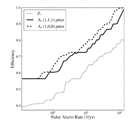
Figure 2: Efficiency in detecting BNS signals versus false-alarm rate computed for various rankings. The solid curve corresponds to the likelihood-ratio ranking, $\Lambda$, with uniform prior $p_{s}(S_{j})=(1,1,1)$. The dashed curve is the likelihood-ratio ranking, $\Lambda$, with the prior $p_{s}(S_{j})=(1,0,0)$, singling out BNS binaries for detection. The dotted curve represents the standard search with the combined effective SNR ranking, $\rho_{\rm eff}$.

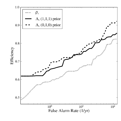
Figure 3: Efficiency in detecting NSBH signals versus false alarm rate computed for various rankings. The solid curve corresponds to the likelihood-ratio ranking, $\Lambda$, with uniform prior $p_{s}(S_{j})=(1,1,1)$. The dashed curve is the likelihood-ratio ranking, $\Lambda$, with the prior $p_{s}(S_{j})=(0,1,0)$, singling out NSBH binaries for detection. The dotted curve represents the standard search with the combined effective SNR ranking, $\rho_{\rm eff}$.

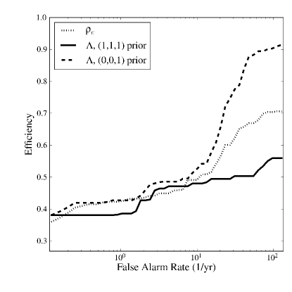
Figure 4: Efficiency in detecting BBH signals versus false alarm rate computed for various rankings. The solid curve corresponds to the likelihood-ratio ranking, $\Lambda$, with uniform prior $p_{s}(S_{j})=(1,1,1)$. The dashed curve is the likelihood-ratio ranking, $\Lambda$, with the prior $p_{s}(S_{j})=(0,0,1)$, singling out BBH binaries for detection. The dotted curve represents the standard search with the combined effective SNR ranking, $\rho_{\rm eff}$.

We apply the new ranking statistic given by Eq. (28) to all triggers: background and signals. Each trigger has three likelihood ratios, one for each binary type. We introduce a prior distribution for binary types, $p_{s}(S_{j})$. It can either encode our knowledge about astrophysical populations of binaries or relative “importance” of different types of binaries to the search. In what follows we consider four alternatives: $p_{s}(S_{j})=(1,0,0)$, $p_{s}(S_{j})=(0,1,0)$, $p_{s}(S_{j})=(0,0,1)$ and $p_{s}(S_{j})=(1,1,1)$. The first three singles out one of the binary types, whereas the last one treats all binaries on equal footing. Finally, the ranking statistic is defined as

$$\Lambda(\rho_{\rm c},\alpha,{\rm m})=\max_{S_{j}}\Lambda(\rho_{\rm c},\alpha,{\rm m}\,|\,S_{j})p_{s}(S_{j})\,.$$ (29)

The four alternative choices for $p_{s}(S_{j})$ define four searches. For example, $p_{s}(S_{j})=(1,0,0)$ corresponds to the search targeting only gravitational-wave signal from BNS coalescence. Similarly, $p_{s}(S_{j})=(0,1,0)$ and $p_{s}(S_{j})=(0,0,1)$ define the searches for gravitational waves from NSBH and BBH. The uniform prior, $p_{s}(S_{j})=(1,1,1)$, allows one to detect all signals without giving priority to one type over the others. In each of the searches, the likelihood-ratio ranking, Eq. (29), re-weights triggers giving higher priority to those that are likely to be the targeted signal as oppose to noise.

In order to assess the improvement attained by the new ranking, we compute efficiency in recovering simulated signals from the data as a function of the rate of false alarms. For a given rate of false alarms we find the corresponding value of the ranking and define efficiency as ratio of injected signals ranked above this value to the total number of signals that passed initial cuts of the analysis pipeline. This is equivalent to computing the standard receiver-operator curve $P_{1}(P_{0})$ defined by Eqs. (4)–(5). The Efficiency curves are computed for BNS, NSBH and BBH binaries. In each case we evaluate efficiency of both likelihood-ratio rankings, the one that targets only that type of binary and the one that applies the uniform prior, $p_{s}(S_{j})=(1,1,1)$. We compare the resulting curves to the efficiency curve for the standard analysis pipeline that uses the combined effective SNR, $\rho_{\rm c}$ as the ranking statistic. These curves are shown in Figures 2–4.

They reveal that the searches targeting single type of binary, represented by the dashed curves, are more sensitive than the uniform search, the solid curve. This is expected, because narrowing down the space of signals typically allows one to discard the triggers that mismatch the signal’s parameters reducing the rate of false alarms without loss of efficiency in recovering these signals. For instance, the search targeting BNS only signals discards all triggers from the high chirp mass bins, $\rm m=2,3$, without discarding the BNS signals. This reduces the rate of false alarms, although at the prices of missing possible gravitational-wave signals from other types of binaries, NSBH and BBH. Still, one could justify such search if it was known that NSBH and BBH binaries do not exist or are very rare. The uniform search, despite being less sensitive to BNS signals, allows one to detect the signals from all kinds of binaries. Such search still gains in efficiency over the standard search, the dotted curve, for BNS and NSBH systems, Figures 2 and  3. At the same time, Figure 4 shows that such search does worse in comparison to the standard search in detecting BBH signals. This is an unavoidable consequence of re-weighting of triggers by the likelihood ratio, Eq. (29) based on their type and chirp mass. It ranks triggers from the lower chirp mass bins higher, because these triggers are less likely to be a noise artifact. This leads to some loss of sensitivity to BBH signals, but gains sensitivity to BNS and NSBH signals. The role of the likelihood ratio is to provide optimal re-weighting of triggers that results in the highest overall efficiency. In the case of the uniform search, it should provide increase in the total number of detected sources of all types. To demonstrate that this is indeed the case, we plotted the combined efficiency of the uniform search for BNS, NSBH and BBH signals and compared it to the efficiency of the standard search, Figure 5.

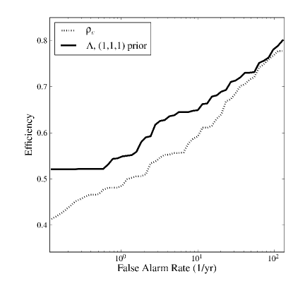
Figure 5: Efficiency in detecting signals from any binary (BNS, NSBH or BBH) versus the false alarm rate computed for various rankings. The solid curve corresponds to the likelihood-ratio ranking, $\Lambda$, with uniform prior $p_{s}(S_{j})=(1,1,1)$. The dotted curve represents the standard search with the combined effective SNR ranking, $\rho_{\rm eff}$.

The combined efficiency of the uniform search on Figure 5 is higher than that of the standard search because triggers are re-weighted by the likelihood ratio which properly accounts for the probability distributions of noise and signals. To gain further insight in this process we pick a particular point on the efficiency curve that corresponds to the rate of false alarms, x-axes, of $1.25$ events per year. We find the corresponding to this rate threshold for combined effective SNR in the standard search to be $\rho_{\rm c}^{*}=11.34$. Next, we find the corresponding threshold for logarithm of the likelihood ratio, $\ln\Lambda^{*}(\rho_{\rm c},\alpha,\rm m)=9.11$. For each $(\alpha,\rm m)$ combination this value can be mapped to $\rho_{\rm c}$ which will be different for each type of trigger. Both $\rho_{\rm c}^{*}=11.34$ and $\ln\Lambda^{*}(\rho_{\rm c},\alpha,\rm m)=9.11$ define detection surfaces in $(\rho_{\rm c},\alpha,\rm m)$ space of trigger parameters. We depicted them on Figure (6).

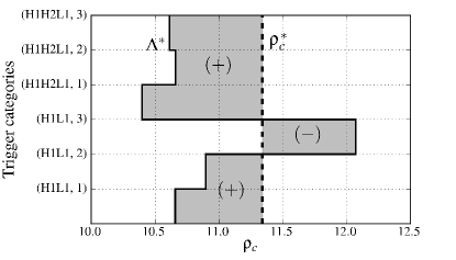
Figure 6: The detection surfaces for the combined effective SNR, $\rho_{\rm{}_{c}}$, and the likelihood-ratio, $\Lambda$, rankings at the false alarm rate of 1.25 events per year. The y-axes labels different types and chirp mass bins of the triggers. The dashed line is the line of constant combined effective SNR, $\rho_{\rm c}^{*}=11.34$. The solid line is the line of constant likelihood ratio, $\ln\Lambda^{*}(\rho_{\rm c},\alpha,\rm m)=9.11$. The signal producing a trigger that falls to the right of the dashed/solid curve is considered to be detected in the search with combined effective SNR/likelihood-ratio ranking. Those triggers that fall to the left are missed. The shaded region is the difference between the detection region for the likelihood-ratio and the combined effective SNR rankings. The signals that produce trigger with parameters in the shaded regions labeled by $(+)$ are gained in the search equipped with likelihood ratio but missed by the search with the combined effective SNR ranking. Those signals that produce a trigger in the shaded region labeled by $(-)$ are missed by the likelihood-ratio ranking but detected by the combined effective SNR ranking.

The signals falling to the right of $\rho_{\rm c}^{*}=11.34$, the dashed line, are considered to be detected in the standard search. Similarly, the signals that happen to produce a trigger to the right of $\ln\Lambda^{*}(\rho_{\rm c},\alpha,\rm m)=9.11$, the solid line, are considered to be detected in the uniform search with the likelihood-ratio ranking. The line of constant likelihood-ratio ranking sets different thresholds for combined effective snr, $\rho_{\rm c}$, of the triggers depending on their type. The threshold is higher than $\rho_{\rm c}^{*}=11.34$ for the H1L1 triggers from the third chirp mass bin. The signals producing triggers in the shaded area in this bin, labeled by $(-)$, are missed in the uniform search but detected by the standard search. These signals are typically corresponds to BBH coalescence. The effect of this is visible on Figure (4), the solid curve is below the dotted curve at false alarm rate of $1.25$ events per year. On the other hand, the thresholds for other trigger types and chirp masses are lower than $\rho_{\rm c}^{*}=11.34$. As a result, the signals producing triggers with parameters in the shaded regions labeled by $(+)$ are detected in the uniform search but missed by the standard one. The net gain from detecting these signals is positive, Figure 5. The process of optimization of the search in $(\rho_{\rm c},\alpha,\rm m)$ parameter space can be thought of as deformation of the detection curve, $\rho_{\rm c}^{*}=11.34$, with the aim of maximizing efficiency of the search. The deformations are constrained to those that do not change the rate of false alarms. The optimal detection surface, as was shown in Section II.2, Eq. (8), is the surface of constant likelihood ratio. This is the essence of likelihood ratio method.

The power of the likelihood-ratio ranking depends strongly on the input data. For demonstration purpose, in the simulation we restricted our attention to a subset of trigger parameters,$(\rho_{\rm c},\alpha,\rm m)$. We expect that inclusion of other parameters such as difference in arrival times of the signal at different detectors, ratios of recovered amplitudes etc, should drastically improve the search. We leave this to future work.

IV Conclusion

In this paper, we describe a general framework for designing optimal searches for transient gravitational-wave signals in data with non-Gaussian background noise. The principle quantity used in this method is the likelihood ratio, the ratio of the likelihood that the observed data contain signal to the likelihood that the data contain only noise. In Section II we prove that the likelihood ratio leads to the optimal analysis of data, incorporating all available information. It is robust against increase of the data volume, effectively ignoring irrelevant information. We apply the general formalism to two typical problems that arise in searches for gravitational-wave signals in LIGO data.

First, in Section III.1 we show that when searching for gravitational-wave signals in the data from different experiments or detector configurations, it is necessary as well as sufficient to rank candidates by the “local” likelihood ratio given by Eq. (22), which is calculated using estimated local probabilities. This provides overall optimality across the experiments. Candidate events from different experiments can be compared directly in terms of their likelihood ratios. This results in complete unification of the data analysis products. Another significant feature of the unified analysis is that the candidate’s significance is independent of the duration of the experiments. Only the detectors’ sensitivities and level of background noise contribute to the likelihood ratio of the candidates. The experiment’s duration, on the other hand, measures its contribution to the total probability of detecting a signal (or efficiency) and the total probability of a false alarm.

Second, in Section III.2 we aim to improve efficiency of the search for gravitational waves from compact binary coalescence by considering the issue of consistent accounting for non-Gaussian features of the noise in the analysis. We suggest a practical solution to this problem. Estimate the probability distributions of parameters of the candidate events (e.g. SNR and the chirp mass of the template waveform, type of trigger etc) in the presence and absence of a signal in the data. Construct the likelihood ratio that includes non-Gaussian features and use it to re-rank candidate events. Non-trivial information contained in the probability distributions of candidate’s parameters allows for a more optimal evaluation of their significance. Indeed, as we demonstrate in the simulation, inclusion of the chirp mass and the type of trigger in the likelihood-ratio ranking results in a significant increase of efficiency in detecting signals from coalescing binaries.

We would like to stress that the approach described in this paper is quite generic and can be applied to wide range of problems in analysis of data with non-Gaussian background. Its main advantage is consistent account of statistical information contained in the data. It provides a unified measure, in the form of the likelihood ratio, of the information relevant to detection of the signal in any type of data. This allows one to combine data of very different kind, such as the type of experiment, a type of trigger, its discrete and continuous parameters etc, into the single optimized analysis.