SPIDER - VI. The Central Dark Matter Content of Luminous Early-Type Galaxies: Benchmark Correlations with Mass, Structural Parameters and Environment

Abstract

We analyze the central dark-matter (DM) content of $\sim 4,500$ massive ($M_{\star}~{}\hbox to0.0pt{$>$\hss}{\lower 4.30554pt\hbox{$\sim$}}10^{10}\,M_{\odot}$), low-redshift ($z<0.1$), early-type galaxies (ETGs), with high-quality $ugrizYJHK$ photometry and optical spectroscopy from SDSS and UKIDSS. We estimate the “central” fraction of DM within the $K$-band effective radius, $R_{\rm eff}$, using spherically symmetric isotropic galaxy models. We discuss the role of systematics in stellar mass estimates, dynamical modelling, and velocity dispersion anisotropy. The main results of the present work are the following: (1) DM fractions increase systematically with both structural parameters (i.e. $R_{\rm eff}$, and Sérsic index, $n$) and mass proxies (central velocity dispersion, stellar and dynamical mass), as in previous studies, and decrease with central stellar density. 2) All correlations involving DM fractions are caused by two fundamental ones with galaxy effective radius and central velocity dispersion. These correlations are independent of each other, so that ETGs populate a central-DM plane (DMP), i.e. a correlation among fraction of total-to-stellar mass, effective radius, and velocity dispersion, whose scatter along the total-to-stellar mass axis amounts to $\sim 0.15$ dex. (3) In general, under the assumption of an isothermal or a constant $M/L$ profile for the total mass distribution, a Chabrier IMF is favoured with respect to a bottom-heavier Salpeter IMF, as the latter produces negative (i.e. unphysical) DM fractions for more than $50\%$ of the galaxies in our sample. For a Chabrier IMF, the DM estimates agree with $\Lambda$CDM toy-galaxy models based on contracted DM-halo density profiles. We also find agreement with predictions from hydrodynamical simulations. (4) The central DM content of ETGs does not depend significantly on the environment where galaxies reside, with group and field ETGs having similar DM trends.

1 Introduction

In the last decade, large area surveys like SDSS (Sloan Digital Sky Survey; Abazajian et al. 2003; Adelman-McCarthy et al. 2008; Abazajian et al. 2009), have provided high quality data contributing significantly to our understanding of galaxy properties and scaling relations. Nevertheless, galaxy formation remains one of the outstanding questions of modern astrophysics. As the most massive stellar systems in the nearby universe, early-type galaxies (ETGs) have a special role in providing the underpinnings for a consistent galaxy formation picture. They form a relatively homogeneous class of objects, dominated by an old stellar population, a small fraction of cold gas and low-levels of ongoing star formation (SF). These characteristics make them a potentially powerful tool to trace the evolution of cosmic structures back through the cosmic epochs. The uniformity in the ETG properties involves tight correlations of quantities like effective radius, $R_{\rm eff}$, surface brightness measured within this radius, and central velocity dispersion, $\sigma_{0}$, which merge into the so-called Fundamental Plane (FP; Djorgovski & Davis 1987; Dressler et al. 1987). An observed deviation between the FP coefficients and those expected from the virial theorem has been interpreted, among other possibilities, as a variation of the total $M/L$  with galaxy luminosity/mass (Dressler et al. 1987) which in turn may reflect the DM content of an ETG (see e.g. Ciotti et al. 1996; Busarello et al. 1997; Graham & Colless 1997; Prugniel & Simien 1997; Trujillo, Burkert & Bell 2004; Cappellari et al. 2006; D’Onofrio et al. 2006; Graves 2009; Tortora et al. 2009, T+09; La Barbera et al. 2010b). Therefore, measuring the DM content in an independent way is of paramount importance for studying the ETG scaling relations as well as the overall process of galaxy formation and evolution. Recently, the DM content in the central regions of ETGs (typically within $1\mbox{$R_{\rm eff}$}$) has been analyzed using both local samples (Padmanabhan et al. 2004; Cappellari et al. 2006; Hyde & Bernardi 2009a; T+09; Napolitano, Romanowsky & Tortora 2010, hereafter NRT10) and intermediate-redshift gravitational lens galaxies (Cardone et al. 2009; Auger et al. 2010b; Cardone & Tortora 2010; Tortora et al. 2010, hereafter T+10; Faure et al. 2011; More et al. 2011). Independent of the model used to describe the mass distribution in a galaxy, several studies have found that DM fractions within $R_{\rm eff}$  increase with galaxy luminosity, stellar mass, size, and velocity dispersion (e.g., Ferreras, Saha, Williams 2005; Cappellari et al. 2006; Forbes et al. 2008; T+09; NRT10; Auger et al. 2010b; Leier et al. 2011; T+10), while a different conclusion was drawn by Trujillo, Burkert & Bell (2004), based on a constant-$M/L$ mass model (see also Grillo 2010). The correlation of DM density with stellar mass and $R_{\rm eff}$  points to DM profiles being cuspy (Thomas et al. 2009; T+09; NRT10; T+10). However, even in this case, inconsistent findings have been reported. Using rotation curves of spiral galaxies, and mass models of individual dwarf and spiral galaxies, as well as the weak lensing signal of ellipticals and spirals, Donato et al. (2009) and Gentile et al. (2009) found that the central DM column density is constant over twelve orders of magnitude in luminosity. On the contrary, NRT10 showed that, on average, the projected central density of nearby ETGs is systematically higher than that of spiral and dwarf galaxies, implying an increase of DM density with halo mass. The same conclusion was reached by Boyarsky et al. (2009), using data for different galaxy types and groups/clusters of galaxies. Part of the above controversies may be associated with sample selection issues, with differences in the way galaxy parameters are measured, as well as with different assumptions about the halo models, IMF, and adopted fiducial radius (Cardone & Tortora, 2010). In this paper, we study how the central DM content of ETGs correlates with galaxy properties, for a large and homogeneous sample with a wealth of photometric and spectroscopic data available (La Barbera et al., 2010a, Paper I of the series). In previous papers, we analyzed the FP relation of ETGs and its dependence on galaxy environment (La Barbera et al. 2010b, Paper II; La Barbera et al. 2010c, Paper III); and the correlation of internal colour gradients of ETGs with galaxy properties (La Barbera et al. 2010b, Paper IV). Here, we investigate the DM content of ETGs in terms of both structural parameters and various mass proxies, contrasting the average trends with predictions of toy-models and cosmological simulations. We show, for the first time, how the correlations between the DM content and galaxy properties depend on the environment where these systems reside. Our study resembles previous ones in its use of SDSS data to study the connections between stellar and dynamical mass (Padmanabhan et al., 2004; Shankar & Bernardi, 2009; Graves & Faber, 2010; Grillo, 2010), but goes beyond these by incorporating additional photometric data as well as environmental information, and may be considered the definitive study of the central DM content of a large sample of bright ETGs in the SDSS era. The outline of the paper is as follows. In Section 2 we describe the sample and the data analysis as well as stellar and dynamical mass calculations. In Section 3, central DM fraction and density are analyzed as a function of galaxy mass and structural parameters. In Section 4 we discuss the main drivers of the DM content and the “DM plane” of ETGs, and in Section 5 the implications for the FP are discussed. Section 6 deals with galaxy environment, while Section 7 compares the correlations involving DM content with expectations from cosmological and toy-galaxy models. Conclusions are presented in Section 8. Throughout the paper, we adopt $H_{0}=75\,\textrm{km}\,\textrm{s}^{-1}\,\textrm{Mpc}^{-1}$.

2 Data sample and analysis

2.1 Sample

A volume-limited sample of $39,993$ “bright” (${}^{0.1}M_{r}<-20$) ETGs, in the redshift range of $0.05$ to $0.095$, with available $ugriz$ photometry and optical spectroscopy from SDSS-DR6 is used in this work and in previous papers of the SPIDER (Spheroid’s Panchromatic Investigation in Different Environmental Regimes) project. $5,080$ galaxies also have $YJHK$ photometry from DR2 of UKIDSS-LAS (see Paper I). ETGs are defined as bulge dominated systems, with passive spectra in their centres (i.e. within the SDSS fibre apertures). Following Bernardi et al. (2003a), from an operational viewpoint, ETGs are those systems with eClass $<0$ and fracDevr $>0.8$, where the SDSS spectroscopic parameter eClass gives the spectral type of a galaxy, while the SDSS photometric parameter fracDevr measures the fraction of galaxy light that is better fitted by a de Vaucouleurs (rather than an exponential) law. All galaxies have central velocity dispersion, $\sigma$, from SDSS-DR6, in the range of $70$ to $420$ km s^-1. In all wavebands, galaxy structural parameters – i.e. the effective radius, $R_{\rm eff}$, the mean surface brightness within that radius, $<\!\mu\!>_{\rm e}$, and the Sérsic index, $n$  – have been homogeneously measured using 2DPHOT (La Barbera et al., 2008a), fitting galaxy images with seeing convolved two-dimensional Sérsic models. The SPIDER sample is $95\%$ complete at ${}^{0.1}M_{r}$$=-20.32$, or, at a stellar mass $M_{\star}=3\times 10^{10}M_{\odot}$ for a Chabrier (2001) IMF.

For the present study, we select SPIDER ETGs with high quality structural parameters in the optical and Near-InfraRed (NIR) wavebands, according to the following criteria: the Sérsic fit has $\chi^{2}<2$ in all wavebands; uncertainty on $\log\mbox{$R_{\rm eff}$}$ $<$ $0.5$ dex from $g$ through $K$ (see Paper IV for details on these thresholds); available stellar mass estimates (Swindle et al. 2011, Paper V). The resulting sample consists of $4,259$ ETGs. As expected, all these galaxies reside on the red-sequence, with more than $99\%$ having $g-r~{}\hbox to0.0pt{$>$\hss}{\lower 4.30554pt\hbox{$\sim$}}0.5$ (within an aperture of 1 $R_{\rm eff}$), and a median $g-r=0.88$. For this sample, the $R_{\rm eff}$ spans the range $\sim(0.5-40)\,\rm kpc$ ( $\sim(1-15)\,\rm kpc$ for more than $90\%$ of the galaxies), with a median of $3.5\,\rm kpc$. The median ratio between the SDSS fibre aperture, where velocity dispersions are measured, and the $K$-band effective radius, $R_{\rm ap}/\mbox{$R_{\rm eff}$}$, amounts to $\sim 0.6$, implying only a little “extrapolation” in our DM fraction estimates (see Sec. 2.3). As shown in Paper I, significant differences are found when comparing 2DPHOT and SDSS structural parameters. Such differences arise from the use of Sérsic (2DPHOT) rather than de Vaucouleurs (SDSS) models to fit the light and total mass distribution of ETGs; from different software to measure the structural parameters; and from the sky estimation bias that affects SDSS photometry (Adelman-McCarthy et al., 2008). In Appendix A, we further illustrate this point by comparing correlations among structural parameters from different sources. The environment of ETGs in the SPIDER sample is characterized by a friends-of-friends catalog of $8,083$ groups, created as in Berlind et al. (2006). Here, we used Berlind’s algorithm over a larger area, as the new SDSS-DR7 is now available (rather than DR3; see Paper III for details). A shifting gapper technique is applied to this catalogue (see Lopes et al. 2009a), allowing galaxies to be classified as either group members ($\sim 46\%$), non-group members (hereafter “field” galaxies; $\sim 33\%$), or unclassified ($\sim 21\%$). We also separate group members into central and satellite galaxies, where the central galaxy of a given group is the object with the largest stellar mass (Yang et al., 2007).

2.2 Stellar mass estimates

Stellar masses are derived by fitting synthetic stellar population (SP) models from Bruzual & Charlot (2003, BC03 hereafter) to the optical+NIR photometry, using the software LePhare (Ilbert et al. 2006). The observed galaxy fluxes determine the normalization of the best-fit template, which then gives the stellar mass, $M_{\star}$ (initially computed within the SDSS Kron aperture, which we correct using Sérsic models to total mass). We adopt a set of SP models with different star-formation $e$-folding times ($\tau\leq 15$ Gyr), internal reddenings ($E(B-V)\leq 0.5$), and metallicities ($0.2\leq Z/Z_{\odot}\leq 3$), assuming a Cardelli et al. (1989) extinction law and Chabrier IMF.

Figure 1: Panel (a). Distributions of $K$ for ${\tt SIS}$ and const-${\tt M/L}$ mass models (see Eq. (1)). Panels (b-e). Median value of $K$ as a function of $\sigma$ (b), $M_{\star}$ (c), $R_{\rm eff}$ (d), and $n$ (e). Median values, with error bars showing 25–75 per cent scatter. Red and blue colours refer to ${\tt SIS}$ and const-${\tt M/L}$ models, respectively. The black curve in panel (e) is taken from Bertin et al. (2002).

We refer the reader to Paper V for all details about the fitting procedure and the accuracy of stellar mass estimates using different theoretical and empirical assumptions. We provide here only a summary of statistical and systematic uncertainties on stellar mass estimates. In paper V, we compared stellar mass estimates obtained with different stellar population models, e.g. BC03 and PEGASE.2 models (Fioc & Rocca-Volmerange, 1997), different internal extinction laws, and different combinations of wavebands adopted in the SED fitting procedure. Also, we performed comparisons with spectroscopically derived stellar masses (the two sets of estimates being in excellent agreement, with a median difference of $0.03\,\rm dex$).

In general, the comparison of different sets of stellar mass estimates shows that the scatter in $M_{\star}$  (i.e. its uncertainty) ranges from $0.05$ to $0.15$ dex. As in other studies (see Paper V and references therein) systematic uncertainties on stellar mass were found to play a major role, with variations in the IMF and extinction law yielding systematic biases on the mass of nearly a factor of 2. Notice though, that despite the age-metallicity degeneracies in photometric data, these conspire to keep the stellar mass-to-light ratio (and hence the stellar masses) relatively well constrained. A de-projected Sérsic law in the $K$-band is used to describe the density profile of the stellar component.

2.3 Dynamical mass estimates

The dynamical mass within a given galaxy radius, $r$, is usually computed as:

$$M_{dyn}=\frac{K\sigma^{2}r}{G},$$ (1)

where $G$ is the gravitational constant, $\sigma$ is the galaxy velocity dispersion, and $K$ is a pressure correction term (e.g. Padmanabhan et al. 2004; Eke et al. 2004; Cappellari et al. 2006; T+09). The $K$ depends on several factors, like the radius wherein $M_{\rm dyn}$  is computed, the aperture used to measure $\sigma$, the viewing angle of the system, its orbital structure, luminosity profile, and how DM is distributed. Here, we follow the approach used in T+09, where instead of adopting some approximation for $K$ in Eq. (1), we model each individual galaxy directly using the Jeans equations to estimate $M_{\rm dyn}$ within $r=$ 1 $R_{\rm eff}$  (see also Cardone & Tortora 2010; T+10). The models also require assumptions about the mass profile in order to extrapolate to $R_{\rm eff}$ from the more central (on average) $\sigma$ measurements. Here our approach is to adopt two types of mass profile that bracket a range of possibilities. Each of these describes the total mass profile with one free parameter:

• SIS. The Singular Isothermal Sphere, where $M(r)\propto\sigma_{\rm SIS}^{2}r$, is the prototype of a galaxy profile producing a flat rotation curve. Despite its simplicity, this reproduces quite well the total mass profile in the most massive ETGs (e.g. Kochanek 1991; Koopmans et al. 2006; Gavazzi et al. 2007), and in particular the massive halo present in their outer regions, consistently with virial mass estimates (Benson et al. 2000; Marinoni & Hudson 2002; Napolitano et al. 2005; van den Bosch et al. 2007). Since a galaxy halo is expected to be truncated when it enters a group/cluster of galaxies, we analyze the impact of the environment on the central DM fractions using also a truncated SIS model (tr-${\tt SIS}$), where the density profile is truncated at a radius $r_{t}$. For each of the group ETGs, the value of $r_{t}$ is computed from the projected distance between the ETG and the centre of the parent group, following the recipes of Ghigna et al. (1998).

• Constant $M/L$. Some studies of ordinary ETGs suggest that the mass profile falls off roughly as steeply as the stars, at small to intermediate radii, which may imply either little DM in their centres or DM profiles that mimic the stars (Romanowsky et al., 2003; Douglas et al., 2007; Deason et al., 2012). The mass profile is given by $M(r)=\Upsilon_{0}\,L(r)$, where $\Upsilon_{0}$ is the typical mass-to-light ratio of the system and $L(r)$ is the luminosity profile, modeled here by the Sérsic (1968) law. Hence, the mass distribution is assumed to follow the profile of the stellar component, whose shape (i.e. the Sérsic $n$), changes from galaxy to galaxy, reflecting the structural non-homology of the light profiles of ETGs.

Operationally, for each galaxy, given a mass profile model, we compute the projected mass-weighted velocity dispersion of the model, $\sigma_{model}$, within the SDSS fibre aperture. The $\sigma_{model}$ is then matched to the observed central velocity dispersion of the galaxy, providing the corresponding best-fit parameter, $\sigma_{\rm SIS}$ ($\Upsilon_{0}$) for the ${\tt SIS}$ (const-${\tt M/L}$) model, and the mass profile $\mbox{$M_{\rm dyn}$}(r)$ (see Appendix B for details).

3 Dynamical masses and central dark matter

We characterize the DM content of an ETG by computing (i) the de-projected DM fraction, $\mbox{$f_{\rm DM}$}(r)=1-\mbox{$M_{\star}$}(r)/\mbox{$M_{\rm dyn}$}(r)$ or the total-to-stellar mass ratio $\mbox{$M_{\rm dyn}$}(r)/\mbox{$M_{\star}$}(r)$, where $M_{\star}$  and $M_{\rm dyn}$  are the stellar and dynamical mass  within a given de-projected radius, $r$; and (ii) the de-projected average DM density, $\mbox{$\langle\rho_{\rm DM}\rangle$}=(\mbox{$M_{\rm dyn}$}(r)-\mbox{$M_{\star}$}(r))/(\frac{4}{3}\pi r^{3})$, giving more direct information on the DM content of a galaxy. The $\mbox{$M_{\star}$}(r)$ is estimated by de-projecting the $K$-band light profile of each galaxy (assuming spherical symmetry), and normalizing this de-projected profile to the total $M_{\star}$  estimate, from Paper V. Hereafter, we refer to $\mbox{$f_{\rm DM}$}(r=R_{e})$ ($\langle\rho_{DM}(r=R_{e})\rangle$), i.e. the DM fraction (density) computed within a de-projected radius equal to the projected $R_{e}$, as the “central” DM fraction (density).

3.1 Dynamical masses and virial coefficients

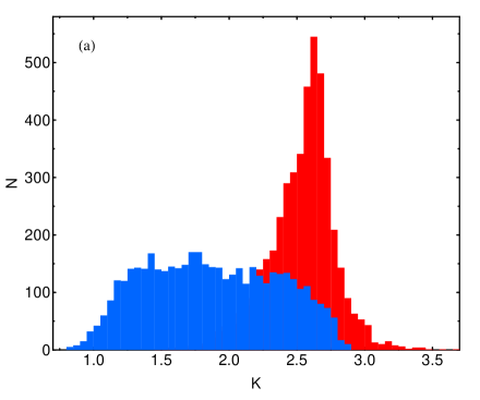
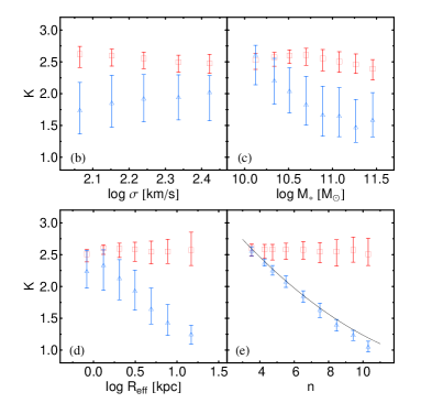
To provide a more straightforward way of estimating $M_{\rm dyn}$ from velocity dispersion and effective radius (as done in previous work), and of comparing mass estimates from different models, we also recast the computation of dynamical masses in terms of Eq. (1). For each galaxy, we correct the observed $\sigma$ to an aperture of 1 $R_{\rm eff}$, $\sigma(\mbox{$R_{\rm eff}$})$, following Cappellari et al. (2006) (see also J$\rm{\o}$rgensen et al. 1995, 1996). Then, we insert $R_{\rm eff}$, $\sigma(\mbox{$R_{\rm eff}$})$, and the dynamical mass estimates obtained through the Jeans equations (see above) into Eq. (1) to obtain the corresponding virial coefficients, $K_{\rm SIS}$ and $K_{\rm M/L}$, for the ${\tt SIS}$ and const-${\tt M/L}$  models, respectively. The distributions of $K_{\rm SIS}$ and $K_{\rm M/L}$ are displayed in the left–panel of Fig. 1, while the right panels show the median values of $K_{\rm SIS}$ and $K_{\rm M/L}$ as a function of $\sigma$, $M_{\star}$, $R_{\rm eff}$, and $n$. The distributions of $K_{\rm SIS}$ and $K_{\rm M/L}$ have median values  of $K_{\rm SIS}=2.57^{+0.11}_{-0.17}$ and $K_{\rm M/L}=1.85^{+0.43}_{-0.38}$ (where error bars are the 25–75 per cent scatter). The $K_{\rm M/L}$ is always smaller than $K_{\rm SIS}$, reaching equality only for galaxies with a $K$-band Sérsic $n\sim 3.5$ (see panel (e) of Fig. 1). This is consistent with the findings in T+09, where galaxy structural parameters were derived using a de Vaucouleurs rather than a Sérsic model. From Fig. 1 we see that $K_{SIS}$ is independent of $\sigma$, $M_{\star}$, $R_{\rm eff}$, and $n$, while $K_{\rm M/L}$ decreases with $M_{\star}$, $R_{\rm eff}$, and $n$, and is independent of $\sigma$. The $K-n$ trend is in fairly good agreement with the best-fitting $K-n$ relation obtained by Bertin et al. (2002) (see solid black line in panel (e)). Notice that using a constant $K_{SIS}$ rather than fitting each individual galaxy with the ${\tt SIS}$  model would introduce an uncertainty in dynamical mass equal to the scatter of the $K_{SIS}$ distribution in Fig. 1, $\sim 4-7\%$ (taking the lower and upper 25–75 per cent range, respectively). Similarly, using the $K-n$ median trend to obtain $K_{\rm M/L}$ would imply an uncertainty of $\sim 4$–$5\%$ on $M_{\rm dyn}$. Modelling each individual galaxy has the advantage of avoiding this source of scatter, which could be important for discerning subtle differences in DM content among different subsamples (e.g. different environments, see Sec. 6).

For group ETGs, we have also computed $K$ values by using the truncated ${\tt SIS}$ model, tr-${\tt SIS}$ (see Sec. 2.3), finding them to be fully consistent with those obtained from the ${\tt SIS}$ model. In particular, only $\mathrel{\hbox to0.0pt{\lower 3.5pt\hbox{\hskip 0.5pt$\sim$}\hss}\raise 0.5pt\hbox{$<$}}2\%$ of group galaxies exhibit a difference of $\Delta\log K>0.01$ ($\sim 2.3\%)$. This is due to the fact that the truncation radius, $r_{t}$ (see Sec. 2.3), has a distribution peaked at $\sim 50$ kpc, with $R_{\rm eff}$ being $\sim 3.5$ kpc, i.e. $\ll r_{t}$.

Throughout the present paper, the DM content of ETGs is estimated under the assumption that their stellar orbits are isotropic, which is incorrect at some level. Although a detailed analysis of anisotropic orbits is far from being trivial, and is certainly beyond the scope of the present work, we have estimated how anisotropy can affect our dynamical mass estimates.

Detailed dynamical modeling efforts of ETGs have focused extensively on their central regions (i.e. those we investigate in this work), and found anisotropies to be fairly mild in general, typically in the range $-0.2\leq\beta\leq+0.3$ (Gerhard et al., 2001; Cappellari et al., 2007), where $\beta\equiv 1-\sigma_{\theta}^{2}/\sigma_{r}^{2}$ quantifies the relative internal dispersions in the tangential and radial directions. Mild central anisotropy is also predicted from simulations of merger remnants (Dekel et al., 2005).

Recent work has focused attention on the ability to constrain $\mbox{$M_{\rm dyn}$}(\mbox{$R_{\rm eff}$})$ in stellar systems, independently of anisotropy, if the velocity dispersion can be measured over the whole galaxy (Walker et al., 2009; Wolf et al., 2010). If the dispersion is measured only within an aperture of $R_{\rm eff}$, but the dispersion profile is relatively constant with radius, it is possible that the mass can still be fairly well constrained (G. Mamon, priv. comm.). To check this, we have carried out test models as in Appendix B, but adopting constant anisotropy profiles, $\beta(r)=\beta$.

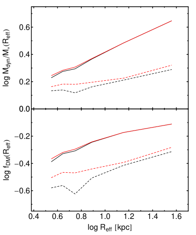
For $\beta=0.1$ ($=0.2$), we find dynamical masses that are $\sim 2\%$ ($\sim 4\%$) smaller than in the isotropic case. In the case of extremely (and indeed unrealistic) radial (tangential) orbits, i.e. $\beta=1$ ($\beta=-1$), the masses are underestimated (overestimated) by $\sim 30\%$ ($\sim 10\%$). The effect is larger for the most massive and largest galaxies in our sample, for which we find that $\beta=0.1$ ($=0.2$) would make the masses smaller by $\sim 3\%$ ($\sim 6\%$), while in the case of $\beta=1$ ($\beta=-1$), the masses would be smaller (larger) by $\sim 50\%$ ($\sim 20\%$). Thus, for typically observed values of $\beta$ ($\sim 0.2$), we do not expect any significant variation in the DM content of ETGs as inferred under the assumption of isotropy, the effect being $\mathrel{\hbox to0.0pt{\lower 3.5pt\hbox{\hskip 0.5pt$\sim$}\hss}\raise 0.5pt\hbox{$<$}}5\%$.

3.2 Dark matter fractions

Figure 2: Dynamical mass within 1 $R_{\rm eff}$ as a function of stellar mass within the same radius. The black solid (dashed) line is the median ${\tt SIS}$ (const-${\tt M/L}$) trend, with the shaded region corresponding to the 25–75 per cent scatter for the ${\tt SIS}$ case. The red lines are the median trends obtained by using only galaxies with $\mbox{$f_{\rm DM}$}\geq 0$. A Chabrier IMF is assumed in the computation of $M_{\star}$ (see Paper V). The solid blue line is the one-to-one relation $\mbox{$M_{\rm dyn}$}(\mbox{$R_{\rm eff}$})=\mbox{$M_{\star}$}(\mbox{$R_{\rm eff}$})$. The arrows show the variation of $M_{\star}$ when adopting a Salpeter, rather than a Chabrier IMF.

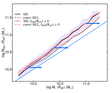
Fig. 2 plots median dynamical masses as a function of stellar mass, $\mbox{$M_{\star}$}(\mbox{$R_{\rm eff}$})$, for both ${\tt SIS}$ and const-${\tt M/L}$  models. We find $\mbox{$M_{\rm dyn}$}(\mbox{$R_{\rm eff}$})\propto\mbox{$M_{\star}$}(\mbox{$R_{\rm eff}$})^{\alpha}$, with $\alpha>1$, i.e. the central DM content increases with galaxy mass. In particular, we find $\alpha_{\rm SIS}\sim 1.2$ and $\alpha_{\rm M/L}\sim 1.07$ for the ${\tt SIS}$  and const-${\tt M/L}$  models, respectively. Notice that on average, at fixed $\mbox{$M_{\star}$}(\mbox{$R_{\rm eff}$})$, the $\mbox{$M_{\rm dyn}$}(\mbox{$R_{\rm eff}$})$ is larger than $\mbox{$M_{\star}$}(\mbox{$R_{\rm eff}$})$, and the fraction of ETGs with $M_{\star}$$>$$M_{\rm dyn}$  (i.e. unphysical DM fractions) is $\sim 12\%$ ($24\%$) for the ${\tt SIS}$  (const-${\tt M/L}$). Using a Salpeter (rather than Chabrier) IMF would shift $M_{\star}$ to larger values by $\sim 0.25$ dex (see the blue arrows in the Figure), making the median $M_{\rm dyn}$ only slightly larger than $M_{\star}$, and increasing the fraction of objects with $M_{\star}$$>$$M_{\rm dyn}$  up to $\sim 55\%$ ($78\%$) for the ${\tt SIS}$  (const-${\tt M/L}$) model.

Taken at face value, this result implies that the bottom-heavy Salpeter IMF is disfavoured with respect to a Chabrier IMF, in agreement with previous findings from stellar dynamics (e.g., Cappellari et al. 2006; NRT10), and from lensing (Ferreras, Saha, Burles, 2008; Ferreras et al., 2010). However, we warn the reader that (i) most of the objects with $M_{\star}$$>$$M_{\rm dyn}$ are from a region of parameter space (low $M_{\star}$) where our sample is more affected by incompleteness (see below); and (ii) our analysis relies on the assumption of a given model for the dynamical mass distribution in ETGs (i.e., either ${\tt SIS}$  or const-${\tt M/L}$). Indeed, if we relax the assumption of a universal IMF, our data would be consistent with either a Salpeter or Chabrier IMF at high mass (T+09, NRT10, Auger et al. 2010a; Treu et al. 2010) and with a Chabrier IMF preferred at low mass (Barnabè et al. 2011; Sonnenfeld et al. 2011; Brewer et al. 2012; Cappellari et al. 2012; Dutton et al. 2012; see also Section 3.3 below).

Figure 3: DM fraction within $R_{\rm eff}$ as a function of $K$-band $R_{\rm eff}$, $n_{\rm K}$, velocity dispersion $\sigma$, stellar mass $M_{\star}$, central average stellar density $\langle\rho_{\rm\star}\rangle$ and dynamical mass, $M_{\rm dyn}$. The symbols are as in Fig. 2. The vertical dotted lines set the completeness limit determined as discussed in the text.

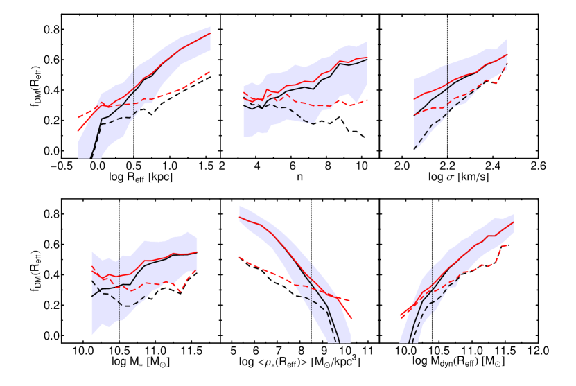
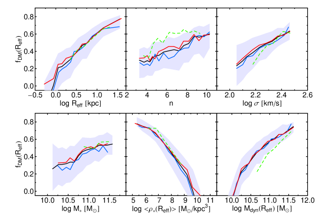
Fig. 3 plots central DM fractions as a function of different galaxy parameters, i.e. effective radius, Sérsic index, velocity dispersion, stellar and dynamical mass, and central average de-projected stellar density, $\langle\rho_{\rm\star}\rangle$, defined as $\mbox{$\langle\rho_{\rm\star}\rangle$}=\mbox{$M_{\star}$}(\mbox{$R_{\rm eff}$})/(\frac{4}{3}\pi\mbox{$R_{\rm eff}$}^{3})$. Black solid (dashed) lines show median trends for the ${\tt SIS}$ (const-${\tt M/L}$) model, while grey regions are the 25–75 per cent quantiles (i.e. the scatter) for the ${\tt SIS}$ model. Notice that, in general, the scatter goes from $\sim 0.2$ at low $f_{\rm DM}$ ($\sim 0.2$) up to $\sim 0.1$ (or smaller) at high $f_{\rm DM}$ ($\sim 0.8$). This is likely caused by the statistical uncertainties on galaxy parameters, such as, in particular, the $M_{\star}$. In fact, a typical statistical uncertainty of $\sim 0.1$ dex on $M_{\star}$  (see Sec. 2.2) propagates into an error of $\sim 0.18$ ($\sim 0.05$) on $f_{\rm DM}$, for $f_{\rm DM}$$\sim 0.2$ ($f_{\rm DM}$$\sim 0.8$).

For each galaxy parameter, we derive the completeness limit of the sample with respect to that parameter by looking at its correlation with the SDSS $r$-band Petrosian magnitude (which is the main parameter used to select SDSS spectroscopic targets; see Papers II and IV for further details on this approach). These completeness limits  are marked by vertical dotted lines in Fig. 3. Notice that because of the scatter around the correlations between $f_{\rm DM}$  and the different galaxy parameters, the range of $f_{\rm DM}$, as seen by the black curves in Fig. 3, is different for different quantities, being larger for $R_{\rm eff}$, $\langle\rho_{\rm\star}\rangle$  and $M_{\rm dyn}$  ($0\mathrel{\hbox to0.0pt{\lower 3.5pt\hbox{\hskip 0.5pt$\sim$}\hss}\raise 0.5pt\hbox{$<$}}\mbox{$f_{\rm DM}$}\mathrel{\hbox to0.0pt{\lower 3.5pt\hbox{\hskip 0.5pt$\sim$}\hss}\raise 0.5pt\hbox{$<$}}0.8$), than for $M_{\star}$, $\sigma$ and $n$ ($0.2\mathrel{\hbox to0.0pt{\lower 3.5pt\hbox{\hskip 0.5pt$\sim$}\hss}\raise 0.5pt\hbox{$<$}}\mbox{$f_{\rm DM}$}\mathrel{\hbox to0.0pt{\lower 3.5pt\hbox{\hskip 0.5pt$\sim$}\hss}\raise 0.5pt\hbox{$<$}}0.6$). All median trends in the Figure are modeled by linear least-squares fits, adopting $\log\mbox{$f_{\rm DM}$}$ as the dependent variable, and using only the portions of each diagram where the sample is complete . In these ranges, the $\log\mbox{$f_{\rm DM}$}$ trends are reasonably well described by the linear fits. The slopes of the best-fitted relations are reported in Table 1, where it should be kept in mind that the range of completeness corresponds to those galaxies which required the most extrapolation from the fibre aperture to $R_{\rm eff}$, so the $f_{\rm DM}$ results are the most model dependent. We also tabulate the slopes obtained by using $\log\mbox{$M_{\rm dyn}$}/\mbox{$M_{\star}$}$, rather than $\log\mbox{$f_{\rm DM}$}$, as the dependent variable in the fits. This is relevant to connect DM fractions to the origin of scaling relations of ETGs (Sec. 5). Notice also, that due to scatter in DM content at a given point of the parameter space, studying $f_{\rm DM}$ is not the same as studying $M_{\rm dyn}$$/$$M_{\star}$. In fact, considering the non-linear relation between $f_{\rm DM}$  and $\mbox{$M_{\rm dyn}$}/\mbox{$M_{\star}$}$, computing the average $\mbox{$M_{\rm dyn}$}/\mbox{$M_{\star}$}$ and plugging it into the definition of $f_{\rm DM}$ is not the same as computing directly the average $f_{\rm DM}$.

Table 1: Slopes of the correlation between $f_{\rm DM}$, $M_{\rm dyn}/\mbox{$M_{\star}$}$ and $\langle\rho_{\rm DM}\rangle$ vs $R_{\rm eff}$, $n$, $\sigma$, $M_{\star}$, $\langle\rho_{\rm\star}\rangle$ and $M_{\rm dyn}$, for the ${\tt SIS}$ and const-${\tt M/L}$ models. We also show in parenthesis the slopes when $M_{\rm dyn}>\mbox{$M_{\star}$}$. The fits are performed taking into account the completeness limits.

	${\tt SIS}$	const-${\tt M/L}$
$\mbox{$f_{\rm DM}$}-\mbox{$R_{\rm eff}$}$	$0.26\pm 0.02$	$0.27\pm 0.05$
	($0.24\pm 0.02$)	($0.18\pm 0.04$)
$\mbox{$f_{\rm DM}$}-n$	$0.39\pm 0.11$	$-0.60\pm 0.11$
	($0.33\pm 0.07$)	($-0.22\pm 0.06$)
$\mbox{$f_{\rm DM}$}-\sigma$	$0.71\pm 0.11$	$1.17\pm 0.18$
	($0.62\pm 0.10$)	($0.84\pm 0.15$)
$\mbox{$f_{\rm DM}$}-\mbox{$M_{\star}$}$	$0.24\pm 0.04$	$0.29\pm 0.06$
	($0.15\pm 0.03$)	($0.07\pm 0.05$)
$\mbox{$f_{\rm DM}$}-\mbox{$\langle\rho_{\rm\star}\rangle$}$	$-0.11\pm 0.01$	$-0.11\pm 0.01$
	($-0.11\pm 0.01$)	($-0.07\pm 0.01$)
$\mbox{$f_{\rm DM}$}-\mbox{$M_{\rm dyn}$}$	$0.28\pm 0.02$	$0.33\pm 0.03$
	($0.27\pm 0.01$)	($0.26\pm 0.03$)
$M_{\rm dyn}/\mbox{$M_{\star}$}-\mbox{$R_{\rm eff}$}$	$0.40\pm 0.03$	$0.16\pm 0.04$
	($0.38\pm 0.03$)	($0.12\pm 0.05$)
$M_{\rm dyn}/\mbox{$M_{\star}$}-n$	$0.27\pm 0.04$	$-0.24\pm 0.05$
	($0.25\pm 0.05$)	($-0.13\pm 0.05$)
$M_{\rm dyn}/\mbox{$M_{\star}$}-\sigma$	$0.78\pm 0.13$	$0.76\pm 0.14$
	($0.69\pm 0.12$)	($0.61\pm 0.13$)
$M_{\rm dyn}/\mbox{$M_{\star}$}-\mbox{$M_{\star}$}$	$0.19\pm 0.03$	$0.10\pm 0.02$
	($0.13\pm 0.03$)	($0.04\pm 0.02$)
$M_{\rm dyn}/\mbox{$M_{\star}$}-\mbox{$\langle\rho_{\rm\star}\rangle$}$	$-0.17\pm 0.01$	$-0.06\pm 0.01$
	($-0.16\pm 0.01$)	($-0.05\pm 0.01$)
$M_{\rm dyn}/\mbox{$M_{\star}$}-\mbox{$M_{\rm dyn}$}$	$0.36\pm 0.03$	$0.23\pm 0.03$
	($0.34\pm 0.02$)	($0.20\pm 0.03$)
$\mbox{$\langle\rho_{\rm DM}\rangle$}-\mbox{$R_{\rm eff}$}$	$-1.91\pm 0.06$	$-2.16\pm 0.09$
	($-1.96\pm 0.06$)	($-2.30\pm 0.09$)
$\mbox{$\langle\rho_{\rm DM}\rangle$}-n$	$-1.70\pm 0.16$	$-4.23\pm 0.22$
	($-1.77\pm 0.14$)	($-3.25\pm 0.12$)
$\mbox{$\langle\rho_{\rm DM}\rangle$}-\sigma$	$1.06\pm 0.61$	$1.88\pm 0.74$
	($0.77\pm 0.43$)	($0.96\pm 0.76$)
$\mbox{$\langle\rho_{\rm DM}\rangle$}-\mbox{$M_{\star}$}$	$-0.91\pm 0.11$	$-0.78\pm 0.18$
	($-1.08\pm 0.08$)	($-1.28\pm 0.12$)
$\mbox{$\langle\rho_{\rm DM}\rangle$}-\mbox{$\langle\rho_{\rm\star}\rangle$}$	$0.70\pm 0.02$	$0.83\pm 0.03$
	($0.71\pm 0.02$)	($0.87\pm 0.03$)
$\mbox{$\langle\rho_{\rm DM}\rangle$}-\mbox{$M_{\rm dyn}$}$	$-1.05\pm 0.08$	$-0.68\pm 0.17$
	($-1.12\pm 0.08$)	($-0.93\pm 0.16$)

In agreement with NRT10 and T+10, we find a tight and positive correlation between ${\tt SIS}$  $f_{\rm DM}$  and $R_{\rm eff}$, which may be interpreted as a physical aperture effect, where a larger $R_{\rm eff}$ subtends a larger portion of a galaxy DM halo (see also Auger et al. 2010b). A steep correlation also holds between DM fraction and Sérsic $n$, namely, galaxies with steeper light profiles have higher central DM fractions. We also find that, independent of the adopted mass proxy (i.e. $\sigma$, $M_{\star}$, $M_{\rm dyn}$), more massive galaxies have the largest DM content ($\mbox{$f_{\rm DM}$}\sim 0.6$), while less massive ones have $f_{\rm DM}$$\sim 0.3$.

These findings are consistent with other results in the literature, based on different samples and methodologies (Padmanabhan et al. 2004; Cappellari et al. 2006; Hyde & Bernardi 2009a; T+09; Cardone & Tortora 2010; NRT10). An exception is the conceptually related SDSS analysis by Grillo (2010), who found a fairly weak $f_{\rm DM}$-$R_{\rm eff}$ and $f_{\rm DM}$-$\sigma$ correlations, and an anti-correlation between $f_{\rm DM}$ and $M_{\star}$. These differences may be attributed to the use of a constant $K$, while our effective $K$ values varied from galaxy to galaxy depending on their individual Sérsic parameters. We also note that Grillo (2010) discussed projected rather than de-projected DM fractions. He converted the SDSS velocity dispersion to a $R_{\rm eff}$/8 circular aperture and adopted an expression for the dynamical mass similar to our Eq. 1 in his equation 4. The $K=\pi$ factor in his equation 4 is equivalent to $K=2$ if the dynamical mass is de-projected, and is slightly lower than the average value $\sim 2.15$ we have reported above. There is also a difference in using $K$-band versus $r$-band effective radii (discussed below) and in other details related to the sample selection (such as the redshift range). Fig. 3 also shows a sharp anti-correlation between DM content and central average stellar density, which has not been reported in the literature so far. Galaxies with denser stellar cores have lower DM fractions (i.e. $\mbox{$f_{\rm DM}$}\sim 0$ at $\rho_{\star}\sim 3\times 10^{9}\,\rm\mbox{$M_{\odot}$}kpc^{-3}$), while $f_{\rm DM}$  values as high as $\sim 0.8$ are found at the lowest densities ($\rho_{\star}\sim 10^{6}\,\rm\mbox{$M_{\odot}$}kpc^{-3}$). This trend results from the fact that, on average, higher stellar densities correspond to smaller effective radii, implying a lower $f_{\rm DM}$. For comparison with previous studies (see Sec. 2.3), Fig. 3 also plots results obtained with the const-${\tt M/L}$ model. The $f_{\rm DM}$ values are still found to increase with $R_{\rm eff}$, but with shallower slope relative to the ${\tt SIS}$, while the trend with the Sérsic $n$ is inverted. The trend with $\sigma$ is also similar to that obtained with the ${\tt SIS}$, but at fixed $\sigma$ the $f_{\rm DM}$ values are smaller by $\sim 0.1$–$0.2$. The const-${\tt M/L}$ model implies no correlation of $f_{\rm DM}$ with stellar mass, and a shallower trend (relative to the ${\tt SIS}$) with both central stellar density and $M_{\rm dyn}$.

From the slope values reported in Table 1, we notice that using either $f_{\rm DM}$ or $\mbox{$M_{\rm dyn}$}/\mbox{$M_{\star}$}$ as the dependent variable in the fits leads to different conclusions about the comparison of ${\tt SIS}$ and const-${\tt M/L}$ trends. For instance, the correlation of $f_{\rm DM}$  with $R_{\rm eff}$ is steeper for const-${\tt M/L}$  than ${\tt SIS}$, while the opposite holds for the $\mbox{$M_{\rm dyn}$}/\mbox{$M_{\star}$}$–$R_{\rm eff}$ correlation. Whilst the use of $f_{\rm DM}$ and $\mbox{$M_{\rm dyn}$}/\mbox{$M_{\star}$}$ is not truly equivalent, because of the scatter in DM content at each point of the parameter space (see above), the apparent discrepancy seen in Table 1 for, e.g., the $f_{\rm DM}$– and $\mbox{$M_{\rm dyn}$}/\mbox{$M_{\star}$}$–$R_{\rm eff}$  relations, is indeed caused by the non-linear relation between $f_{\rm DM}$  and $\mbox{$M_{\rm dyn}$}/\mbox{$M_{\star}$}$: a difference in $M_{\rm dyn}$/$M_{\star}$  (such as that between ${\tt SIS}$  and const-${\tt M/L}$ models) corresponds to a smaller difference in $f_{\rm DM}$ at higher, relative to lower, $M_{\rm dyn}$/$M_{\star}$ (i.e. going from low- to high-$R_{\rm eff}$ values). See also Fig. 4 where this effect is make clear by plotting $f_{\rm DM}$– and $\mbox{$M_{\rm dyn}$}/\mbox{$M_{\star}$}$–$R_{\rm eff}$ relations.

Figure 4: $M_{\rm dyn}/\mbox{$M_{\star}$}$ (top panel) and $f_{\rm DM}$ (bottom panel) within $R_{\rm eff}$ in terms of $R_{\rm eff}$ for a ${\tt SIS}$ and const-${\tt M/L}$. The plot is limited to the region where the sample is complete. The symbols are as in Fig. 2 and 3.

The red curves in Fig. 3 also show how median $f_{\rm DM}$ trends change when one excludes objects with $\mbox{$M_{\rm dyn}$}<\mbox{$M_{\star}$}$, i.e. $\mbox{$f_{\rm DM}$}<0$. Except for the trend with $n$ where a small rigid offset is seen ($\sim 0.05$ for the ${\tt SIS}$), all correlations are only affected at one end, i.e. at low mass, velocity dispersion, and $R_{\rm eff}$, and at high $\langle\rho_{\rm\star}\rangle$, where our sample turns out to be incomplete (see above). Hence, the issue of negative $f_{\rm DM}$  values only produce a slight effect on the slopes reported in Tab. 1.

Notice that negative $f_{\rm DM}$  values can be caused by measurement errors on galaxy parameters (i.e. $\sigma$, $R_{\rm eff}$, and $M_{\star}$), a failure of the mass model to estimate $M_{\rm dyn}$, and/or some systematics in the stellar mass estimates, such as the assumption of a given IMF (see Sec. 3.3). In order to assess if these effects can fully account for the negative $f_{\rm DM}$ values in our sample, for each $M_{\star}$, we assign a mock $M_{\rm dyn}$ value, according to the $M_{\rm dyn}$–$M_{\star}$  relation of Fig. 2 (for a ${\tt SIS}$  model). Shifting the $M_{\star}$ and mock $M_{\rm dyn}$  values according to the estimated statistical uncertainties on these quantities ($\sim 0.1$ dex and $0.18$ dex, respectively), we find $\sim 2\%$ of data-points to have $M_{\rm dyn}$$<$$M_{\star}$. This fraction rises to $\sim 12\%$ (i.e., what we actually measure for the ${\tt SIS}$  model), if stellar masses are overestimated by a factor of $1.6$, which is within the factor of $2$ systematic uncertainty on $M_{\star}$  due to different effects (i.e. mainly the extinction law and IMF; see Sec. 2.2 and Paper V).

An alternative explanation for the unphysical $f_{\rm DM}$ values is the choice of the galaxy mass profile, which could be inappropriate for (some) low mass galaxies. For instance, dynamical masses would become systematically larger (than the ${\tt SIS}$ ones) if a power-law density profile, $\rho(r)\propto r^{-\alpha}$ with $\alpha<2$, is adopted (with $M(r)\propto r^{3-\alpha}$, i.e. a mass profile shallower than the ${\tt SIS}$). Different observations have argued that the (dynamical) mass profile of a galaxy might change as a function of its stellar mass. In particular, as already pointed out in Sec. 2.3, massive ETGs are quite well reproduced by nearly-isothermal profiles (e.g. Kochanek 1991; Koopmans et al. 2006; Gavazzi et al. 2007), while in some intermediate-mass ETGs the mass is found to follow the light (Romanowsky et al. 2003; Napolitano et al. 2005; Douglas et al. 2007; Deason et al. 2012). Similarly, non-homology of the mass profiles has also been suggested by T+09. Qualitatively, this would make the trends of $f_{\rm DM}$ in terms of $R_{\rm eff}$, $\sigma$, $M_{\star}$ and $M_{\rm dyn}$ steeper with respect to the case of a pure ${\tt SIS}$ model, and shallower (or inverted) for the cases of $f_{\rm DM}$ versus stellar density and Sérsic index.

Figure 5: $f_{\rm DM}$ within $g$-band $R_{\rm eff}$ in terms of $R_{\rm eff}$, $M_{\star}$ and $M_{\rm dyn}$ for a ${\tt SIS}$. Solid curves and shaded regions are for our sample, as in Fig. 2, while points with error bars are from T+09 and NRT10. The vertical dotted lines mark the completeness limits as in Fig. 3.

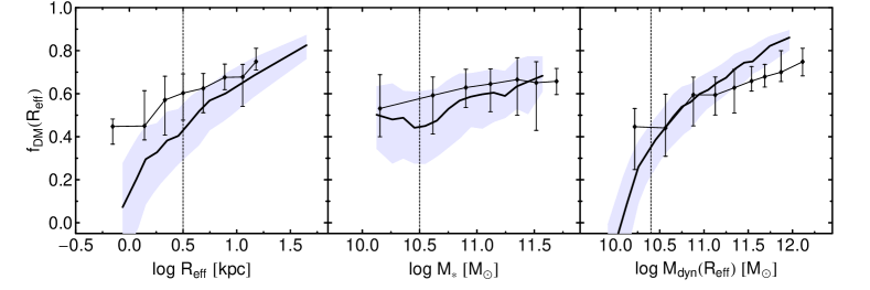
Whilst most of these results are qualitatively consistent with those found in the (recent) literature, one should notice that, in contrast to previous studies, our DM fractions are computed within the $K$-band (rather than optical) effective radius. Hence, our $f_{\rm DM}$ estimates are less affected by the existence of metallicity and age gradients in ETGs, dust extinction and (low fractions of) young stars. In order to permit a more direct comparison with results from our previous work (T+09), we recomputed ${\tt SIS}$ $f_{\rm DM}$ estimates using $g$-band (rather than $K$-band) $R_{\rm eff}$ values. Fig. 5 compares the resulting $g$-band median trends with the $B$-band trends obtained from T+09. For the trend with stellar mass, we find good agreement between the present and our previous work. However, the plots of $f_{\rm DM}$ vs. $R_{\rm eff}$ and $M_{\rm dyn}$ reveal some discrepancies. At low $R_{\rm eff}$ and $M_{\rm dyn}$, the present sample becomes incomplete and we miss galaxies with high $f_{\rm DM}$. This biases our trends towards lower $f_{\rm DM}$ values with respect to T+09. At high $R_{\rm eff}$, our $R_{\rm eff}$ values are larger than those of T+09 (because of the different way structural parameters are estimated; see App. A), explaining the shift of the $f_{\rm DM}$ vs. $R_{\rm eff}$ trend towards larger $R_{\rm eff}$ with respect to T+09. On the other hand, the present $f_{\rm DM}$ vs. $M_{\rm dyn}$ trend is shifted towards lower $M_{\rm dyn}$ values relative to T+09, implying that some further systematic differences exist between the $M_{\rm dyn}$ estimates of the two datasets. Understanding the origin of such differences is far from trivial as we do not have galaxies in common between the two samples. Differences might exist because of different sample selection criteria, and/or different methods used to estimate velocity dispersions.

Figure 6: Trends of $M_{\rm dyn}$/$M_{\star}$  as a function of $K$-band $R_{\rm eff}$, stellar mass $M_{\star}$  (assuming a Chabrier IMF), velocity dispersion, and dynamical mass, $M_{\rm dyn}$. Black curves and grey regions are the same as in Figs. 2 and 3. Horizontal lines correspond to the relative variation of stellar mass, $M_{\star,\rm IMF}/M_{\star}$ – with respect to a Chabrier IMF – when adopting different IMFs, with slopes $1.35$ (i.e. a Salpeter IMF; blue), $1.85$ (green), and $2.05$ (cyan). The red line corresponds to the case of a Chabrier IMF ($M_{\star,\rm IMF}=M_{\star}$). The vertical dotted lines set the completeness limit as in Figs. 3 and 5. For $f_{\rm DM}$$=M_{\star,\rm IMF}/M_{\star}$, one can find the IMF slope that would make $M_{\star}$  equal to $M_{\rm dyn}$, resulting in a galaxy with no DM.

3.3 Constraints on IMF

The present analysis is based on the assumption that the stellar IMF is universal, at least within the parameter range covered by our sample. In principle, for each given galaxy, one could adjust the IMF so that $M_{\star}$=$M_{\rm dyn}$ (or, equivalently, $f_{\rm DM}$$=0$). However, since $f_{\rm DM}$  correlates with various galaxy parameters, any adjustment of the IMF would imply that the IMF itself changes systematically with these parameters, in the same way as $f_{\rm DM}$ (Cappellari et al. 2012). Motivated by the recent claim that the IMF depends on galaxy velocity dispersion (van Dokkum & Conroy, 2011, hereafter vDC11), with high- (relative to low-) $\sigma$ ellipticals having a bottom-heavier IMF, we explore to what extent one can change the IMF in order to fulfill the condition $f_{\rm DM}$$=0$.

We estimate the expected variation of stellar mass, $M_{\star,\rm IMF}/M_{\star}$, relative to a Chabrier IMF, when different IMFs are adopted. Here, $M_{\star}$ is the stellar mass estimated with a Chabrier IMF, while $M_{\star,\rm IMF}$ is the stellar mass we would estimate with a different IMF. In practice, we consider three power-law IMFs, with slopes $1.35$ (i.e. Salpeter), $1.85$, and $2.05$ (i.e. a very bottom-heavy IMF, as suggested by vDC11 for high-$\sigma$ ellipticals). The $M_{\star,\rm IMF}/M_{\star}$ is estimated as the ratio of the stellar $M/L$ between two SSPs having a power-law and a Chabrier IMFs, respectively. To compute the stellar $M/L$, we adopt the BC03 synthesis code, for old ($10$ Gyr) SSPs, with solar metallicity.

Fig. 6 plots the $M_{\rm dyn}$/$M_{\star}$ trends as a function of $R_{\rm eff}$, $M_{\star}$, $M_{\rm dyn}$, and $\sigma$ (black curves), with horizontal lines marking $M_{\star,\rm IMF}/M_{\star}$ for the different IMFs. The intersections of the horizontal lines with the black curves define the values of $R_{\rm eff}$, $M_{\star}$, $M_{\rm dyn}$, and $\sigma$, for which a given IMF slope would imply $f_{\rm DM}$$=0$. The Figure shows that in order to account for the apparent trend of $f_{\rm DM}$ with $R_{\rm eff}$  (and $M_{\rm dyn}$), galaxies with the largest radii (and dynamical masses) should have an IMF slope as steep as $2.05$, while at the lowest $R_{\rm eff}$ (and $M_{\rm dyn}$) a Chabrier (or even a bottom-lighter) IMF would be required. Interestingly, at high velocity dispersion ($\log\sigma\sim 2.45$), we see that the IMF slope cannot be larger than $\sim 1.8$, which seems to contrast with the finding of vDC11, but is in good agreement with Cappellari et al. (2012) (see their no-DM case).

The exercise described so far shows that the estimated trends of $f_{\rm DM}$ might be significantly biased if the IMF varies substantially as a function of different galaxy parameters. However, it remains unclear if and (more importantly) why such correlated variation of IMF slope with different parameters should be present. Another key to the $f_{\rm DM}$ trends might be alternative gravity (Cardone et al. 2011; Lubini et al. 2011; Richtler et al. 2011; Napolitano et al. 2012), which, anyway, is beyond the scope of the present work.

3.4 Dark matter densities

Following T+09 and NRT10, we also analyze the average central DM density of ETGs, $\langle\rho_{\rm DM}\rangle$. The $\langle\rho_{\rm DM}\rangle$ values may be considered the fossil record of the ambient density at the time of initial halo collapse, modulo possible mass-redistributing interactions between DM and baryons. While $f_{\rm DM}$ is defined relative to the baryon mass, $\langle\rho_{\rm DM}\rangle$ quantifies the properties of the DM component alone, allowing for more direct comparisons to cosmological models (see Sec. 7).

Figure 7: Average central DM density as a function of $K$-band $R_{\rm eff}$, $n$, velocity dispersion $\sigma$, stellar mass $M_{\star}$, central average stellar density $\langle\rho_{\rm\star}\rangle$ and dynamical mass, $M_{\rm dyn}$. The symbols are as in Figs. 2 and 3, except as for the red curves in that plot, here only the galaxies with $M_{\rm dyn}>\mbox{$M_{\star}$}$ are used. The vertical dotted lines set the completeness limit as in Figs. 3 and 5.

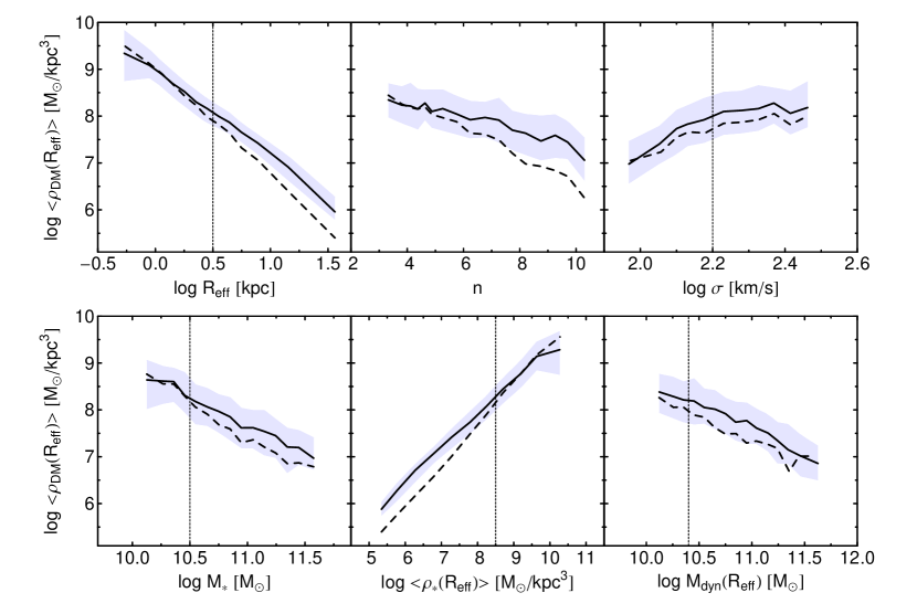
Fig. 7 is the same as Fig. 3, but plotting $\langle\rho_{\rm DM}\rangle$, rather than $f_{\rm DM}$, as a function of structural parameters and galaxy mass proxies. The correlations are again fitted with linear relations, taking into account the completeness limit of each diagram, with the slopes reported in Table 1. We find that $\langle\rho_{\rm DM}\rangle$ decreases with $R_{\rm eff}$, $n$, $M_{\star}$, and $M_{\rm dyn}$. The best-fitting power laws are consistent with results from the literature (Thomas et al. 2009; T+09; NRT10; Auger et al. 2010b; T+10). On the other hand, $\langle\rho_{\rm DM}\rangle$ increases with $\sigma$ and $\langle\rho_{\rm\star}\rangle$. All trends are qualitatively independent of the adopted mass model, although in general the const-${\tt M/L}$ profile produces steeper correlations than the ${\tt SIS}$. As shown in Fig. 7, at low $R_{\rm eff}$, $n$, $\sigma$, $M_{\rm dyn}$, and high $\langle\rho_{\rm\star}\rangle$, $\langle\rho_{\rm DM}\rangle$ is model independent, while the discrepancy between ${\tt SIS}$ and const-${\tt M/L}$ models is larger at high $R_{\rm eff}$, $n$, $\sigma$, $M_{\rm dyn}$, and low $\langle\rho_{\rm\star}\rangle$, making the const-${\tt M/L}$ correlations steeper. This is due to the increasingly important role of mass profile extrapolation in these regimes.

Under the assumption that DM density profiles are universal, at least for all galaxies in our samples, we confirm the result of NRT10, that DM profiles in ETGs are very cuspy, with $\rho_{DM}(r)\sim r^{-2}$. This conclusion is reached as follows. For a power-law DM density distribution, $\rho_{DM}(r)\propto r^{-\alpha}$, we have $M_{DM}=r^{3-\alpha}$ (for $\alpha<3$ ). It follows that $\mbox{$\langle\rho_{\rm DM}\rangle$}(\mbox{$R_{\rm eff}$})\propto\mbox{$R_{\rm eff}$}^{-3}M_{DM}(\mbox{$R_{\rm eff}$})\propto\mbox{$R_{\rm eff}$}^{-\alpha}$. Since the slope of the $\langle\rho_{\rm DM}\rangle$  – $R_{\rm eff}$ correlation is $\sim 2$ for both ${\tt SIS}$  and const-${\tt M/L}$, we conclude that $\alpha\sim 2$, independent of the adopted mass model. This conclusion relies on the assumption that trends in the average values of $\langle\rho_{\rm DM}\rangle$ reflect trends in the mass profiles of individual galaxies (cf. Walker et al. 2009; NRT10). We will return to further implications of this assumption in Section 7.

4 “Dark matter plane” of ETGs

Table 2: Comparison of the $\mbox{$f_{\rm DM}$}-X$ and $\mbox{$f_{\rm DM}$}-\mbox{$\langle Y\rangle$}$ relations (black and red curves in Fig. 8; see the text). We flag with ‘Yes’ (‘No’) those cases where $\mbox{$f_{\rm DM}$}-\mbox{$\langle Y\rangle$}$ overlaps (does not overlap) with $\mbox{$f_{\rm DM}$}-X$.

	$Y^{\prime}$
	$R_{\rm eff}$	$M_{\star}$	$n$	$\sigma$	$\langle\rho_{\rm\star}\rangle$
$X=\log\mbox{$R_{\rm eff}$}$	$-$	No	No	No	Yes
$X=\log\mbox{$M_{\star}$}$	No	$-$	No	Yes	Yes
$X=n$	Yes	No	$-$	No	Yes
$X=\log\sigma$	No	No	No	$-$	No
$X=\log\mbox{$\langle\rho_{\rm\star}\rangle$}$	Yes	No	No	No	$-$

Figure 8: Tests performed to establish the observed ETGs’ parameters driving the correlations with central DM fraction. Each panel shows the observed correlation between $f_{\rm DM}$ and a given parameter $X$ (black solid curve), as well as the correlation expected from that of $f_{\rm DM}$ and another galaxy parameter $Y$ (i.e. $Y\neq X$), and that between $Y$ and $X$ (red solid curve). Each row in the plot corresponds to a given $X$, out of $R_{\rm eff}$, $M_{\star}$, $n$, $\sigma$, and $\langle\rho_{\rm\star}\rangle$ (from top to bottom). For a given row, the panels show the same $f_{\rm DM}$–$X$ correlation (black) and that expected by varying $Y$ (from left to right). For each panel, the corresponding $Y$ is reported in the upper–right corner.

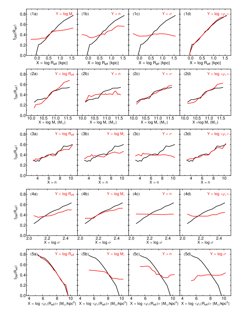
Some of the correlations discussed so far, between DM fraction (density) and different galaxy parameters, could in principle be secondary in nature, arising simply from mutual correlations among the galaxy parameters themselves. For instance, given the $f_{\rm DM}$-$R_{\rm eff}$  relation, a correlation between $f_{\rm DM}$ and stellar mass is also expected to exist, just because of the size–stellar mass relation (e.g. Shen et al. 2003). Therefore we seek to determine the fundamental parameters that relate to the DM matter content of ETGs. We follow the same procedure adopted in La Barbera et al. (2010d) (Paper IV) to establish the main drivers of correlations among internal colour gradients and other observed parameters of ETGs. As illustrated in Fig. 8, we consider a given galaxy parameter, $X$, out of the quantities $\{$$R_{\rm eff}$, $n$, $\sigma$, $M_{\star}$, and $\langle\rho_{\rm\star}\rangle$$\}$ (from top to bottom in the Figure), and the corresponding correlation with $f_{\rm DM}$, $\mbox{$f_{\rm DM}$}(X)$ (black curves in each panel). For a given bin of $X$, we compute the median value ($\langle Y\rangle$) of another galaxy parameter, $Y$, with $Y\neq X$, and then, given the $f_{\rm DM}$$(Y)$ correlation, we compute $\mbox{$f_{\rm DM}$}(\mbox{$\langle Y\rangle$})$ (red curves in the Figure). The $\mbox{$f_{\rm DM}$}(\mbox{$\langle Y\rangle$})$ is the correlation between $f_{\rm DM}$ and $X$ expected from the correlation between $f_{\rm DM}$ and $Y$, and the correlation between $X$ and $Y$ themselves. Each row in Fig. 8, from top to bottom, corresponds to a given $X$, while the panels from left to right show the $\mbox{$f_{\rm DM}$}(\mbox{$\langle Y\rangle$})$ (see red curves) by varying $Y$. If a given $\mbox{$f_{\rm DM}$}(\mbox{$\langle Y\rangle$})$ differs from $\mbox{$f_{\rm DM}$}(X)$ (i.e. the black and red curves in the corresponding panel do not overlap), we can conclude that the correlation between $f_{\rm DM}$  and $X$ is more than just a reflection of one between $f_{\rm DM}$ and $Y$. We evaluate by visual inspection whether or not two curves differ, as summarized in Table 2, for each pair of $X$ and $Y$. We find that the correlation between $f_{\rm DM}$ and $X=\log\mbox{$M_{\star}$}$ (panels 2a–2d) is equivalent to that expected from either $f_{\rm DM}$ and $\sigma$ (panel 2c), or $f_{\rm DM}$ and $\langle\rho_{\rm\star}\rangle$ (panel 2d), i.e. stellar mass is likely not a genuine driver of the DM fraction in ETGs. In the same way, the correlation with Sérsic $n$ is equivalent to that expected between $f_{\rm DM}$ and $R_{\rm eff}$ (or $\log\mbox{$\langle\rho_{\rm\star}\rangle$}$) (panels 3a and 3d). On the contrary, the correlation between $f_{\rm DM}$ and $\sigma$ is a genuine one, as all the red curves in panels 4a–d of Fig. 8 differ, being flatter than the observed $f_{\rm DM}$$(\log\sigma)$. Finally, we see that the $f_{\rm DM}$$(\log\mbox{$R_{\rm eff}$})$ and $f_{\rm DM}$$(\log\mbox{$\langle\rho_{\rm\star}\rangle$})$ correlations are completely equivalent to each other , and are not caused by any correlation of $f_{\rm DM}$ with some other parameter. Since $\rho_{\star}$ is computed from $R_{\rm eff}$, we conclude that the main parameters driving DM fractions are galaxy size and central velocity dispersion. The same result holds when repeating the above analysis using DM density, rather than $f_{\rm DM}$.

Since there are two observed parameters driving the DM content of ETGs ($R_{\rm eff}$ and $\sigma$), we analyze here the correlation of DM with both quantities, using ${\tt SIS}$–based DM estimates. Here, we adopt the logarithmic ratio of dynamical to stellar mass, $\log\,(\mbox{$M_{\rm dyn}$}/\mbox{$M_{\star}$})$. This avoids the issue of negative $f_{\rm DM}$ values and can provide a more direct connection to the FP relation (see § 5). We consider a DM plane relation:

$$\log\frac{M_{\rm dyn}}{\mbox{$M_{\star}$}}=a_{\rm DM}\log\mbox{$R_{\rm eff}$}+b_{\rm DM}\log\sigma_{e}+c_{\rm DM},$$ (2)

where $a_{\rm DM}$ and $b_{\rm DM}$ are the slopes, and $c_{\rm DM}$ is the offset. We perform a linear best-fit of $\log\,(\mbox{$M_{\rm dyn}$}/\mbox{$M_{\star}$})$ vs. $\log\mbox{$R_{\rm eff}$}$ and $\sigma(\mbox{$R_{\rm eff}$})$, minimizing the sum of absolute residuals along the $M_{dyn}/\mbox{$M_{\star}$}$ axis. This gives $a_{\rm DM}=0.380\pm 0.008$, $b_{\rm DM}=0.647\pm 0.03$, $c_{\rm DM}=-1.38\pm 0.06$ (where errors are $1\sigma$ statistical uncertainties). Both $a_{\rm DM}$ and $b_{\rm DM}$ are significantly different from zero, implying that DM content is indeed a function of both $R_{\rm eff}$ and $\sigma$, consistent with what we found above (i.e. that the correlation of $f_{\rm DM}$ and $R_{\rm eff}$ is not equivalent to that with $\sigma$, and vice-versa). Fig. 9 compares the (logarithmic) correlations of $M_{dyn}/\mbox{$M_{\star}$}$ vs. $R_{\rm eff}$ (top), $M_{dyn}/\mbox{$M_{\star}$}$ vs. $\sigma(\mbox{$R_{\rm eff}$})$ (middle), and those between $M_{dyn}/\mbox{$M_{\star}$}$ and both $R_{\rm eff}$ and $\sigma(\mbox{$R_{\rm eff}$})$ (i.e. the DM plane; see bottom panel). See the slopes reported in Table 1. For all panels, the red lines are the best-fitting relations obtained by the same kind of fitting procedure, i.e. minimizing the sum of absolute residuals along the $M_{dyn}/\mbox{$M_{\star}$}$ axis. A robust estimate of the rms along the $M_{dyn}/\mbox{$M_{\star}$}$ axis is also reported in the Figure for each correlation. Notice that the scatter of the DM plane ($\rm rms=0.149\pm 0.002$) is smaller (albeit by a few percent) than that of the $M_{dyn}/\mbox{$M_{\star}$}-\sigma(\mbox{$R_{\rm eff}$})$ ($\rm rms=0.200\pm 0.002$) and $M_{dyn}/\mbox{$M_{\star}$}-\mbox{$R_{\rm eff}$}$ ($\rm rms=0.165\pm 0.002$) correlations.

Figure 9: DM fundamental plane. Top Panel. $\log\mbox{$M_{\rm dyn}$}/\mbox{$M_{\star}$}$ as a function of $R_{\rm eff}$. Middle Panel. $\log\mbox{$M_{\rm dyn}$}/\mbox{$M_{\star}$}$ as a function of $\sigma_{e}$. Bottom Panel. $\log\mbox{$M_{\rm dyn}$}/\mbox{$M_{\star}$}$ as a function of the combination $a_{\rm DM}\log\mbox{$R_{\rm eff}$}+b_{\rm DM}\log\sigma_{e}+c_{\rm DM}$. The cyan lines are the medians, while the red ones are the best fits.

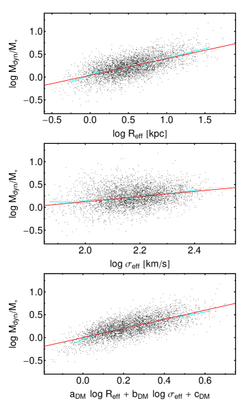
Projecting the $M_{dyn}/\mbox{$M_{\star}$}$ rms along the $\log\mbox{$R_{\rm eff}$}$ axis, we find a scatter of $\sim 0.4$ dex, i.e. much larger than that of the FP relation ($\sim 0.1$ dex; see Paper II). This large dispersion implies that the coefficients of the DM plane depend significantly on the fitting procedure one adopts to derive them. For instance, minizing the rms of absolute residuals along $\log\mbox{$R_{\rm eff}$}$, we find $a_{\rm DM}\sim 0.84$ and $b_{\rm DM}\sim 0.78$, which are significantly different from those obtained from the $M_{dyn}/\mbox{$M_{\star}$}$ best-fit (see above). The scatter of the DM plane decreases to $\sim 0.25$ dex along $\log\mbox{$R_{\rm eff}$}$, still significantly larger with respect to the FP.

5 Dark matter fractions and Fundamental Plane

The correlations of DM content with galaxy parameters might help to shed light on the origin of scaling relations of ETGs, i.e. the tilt of the FP relation. The FP can be written as

$$\log\mbox{$R_{\rm eff}$}=a_{FP}\log\sigma+b_{FP}\langle\mu_{\star}\rangle_{e}+\,constant,$$ (3)

where $a_{FP}$ and $b_{FP}$ are the slopes, and $\langle\mu_{\star}\rangle_{e}$ is the mean surface brightness within $R_{\rm eff}$. Under the assumption of homology, the tilt can be parameterized as a variation of $\mbox{$M_{\rm dyn}$}/L$ with luminosity or mass, i.e. $\mbox{$M_{\rm dyn}$}/L\propto L^{\alpha}$ (Dressler et al. 1987), or $\mbox{$M_{\rm dyn}$}/L\propto{\tt\mbox{$M_{\rm dyn}$}}^{\gamma}$ (with $\gamma=\alpha/(1+\alpha)$). The $M/L$ can be rewritten as

$$\frac{\mbox{$M_{\rm dyn}$}}{L}\propto\frac{\mbox{$M_{\rm dyn}$}}{\mbox{$M_{\star}$}}\frac{\mbox{$M_{\star}$}}{L},$$ (4)

where $\mbox{$M_{\star}$}/L$ is the stellar mass-to-light ratio. In the $K$-band, stellar population effects make a negligible contribution to the tilt (La Barbera et al. 2010b), implying that non-homology and/or a variation of DM content (i.e. $\mbox{$M_{\rm dyn}$}/\mbox{$M_{\star}$}$ changing with luminosity/mass) should explain the tilt. Fig. 3 shows that the central DM content of ETGs does actually change significantly with mass and luminosity. In particular, we find $\mbox{$M_{\rm dyn}$}/\mbox{$M_{\star}$}\propto\mbox{$M_{\rm dyn}$}^{0.36\pm 0.03}$, or $\gamma=0.36\pm 0.03$ (see Table 1). This value is somewhat larger than that found by some previous studies, i.e. $\gamma\sim 0.15$–$0.20$, (Hyde & Bernardi 2009a, Gallazzi et al. 2006 and T+09), possibly due to differences in the way structural parameters are estimated from different sources (see App. A). The value of $\gamma$, as obtained by fitting the $\mbox{$M_{\rm dyn}$}/\mbox{$M_{\star}$}$ vs. $M_{\rm dyn}$ relation, is close to that inferred from FP coefficients, using the virial theorem under the assumption of homology ($\gamma\sim 0.2$; see, e.g., T+09; La Barbera et al. 2010b). This means that DM content variation might be able by itself to explain the entire fraction of the tilt which is not due to stellar population effects (i.e. a variation of age and/or metallicity with mass). We also notice that, in the context of the const-${\tt M/L}$  model, the variation of DM content with mass is flatter than with the ${\tt SIS}$ model, which would lead one to conclude that both non-homology and a change of DM content contribute to the tilt (see T+09 for details). Last, but not least, one should notice that connecting the slope of the $\mbox{$M_{\rm dyn}$}/\mbox{$M_{\star}$}$ vs. $M_{\rm dyn}$ relation to the tilt of the FP is not trivial. The dynamical mass entering the virial theorem is actually the total mass of a galaxy, i.e. all the gravitationally bound matter of the system. Hence, the difference of FP coefficients from the virial theorem expectation might be more related to the total, rather than central ($<1$ $R_{\rm eff}$), DM content of ETGs. Unfortunately, estimating total, rather than central, DM fractions requires a large extrapolation of the central velocity dispersion, much more dependent on the mass model one assumes to infer our default $M_{\rm dyn}$ values. With this caveat in mind, we try here to establish a connection between the DM plane and the FP, combining Eq. (2) with the following expression of the virial theorem, obtained under the assumption of homology (whereby kinetic energy is $\propto M_{dyn}\sigma^{2}$ and potential energy is $\propto M_{dyn}^{2}/\mbox{$R_{\rm eff}$}$):

$$\sigma^{2}\propto G\frac{\mbox{$M_{\rm dyn}$}}{\mbox{$M_{\star}$}}\frac{\mbox{$M_{\star}$}}{\mbox{$R_{\rm eff}$}},$$ (5)

where $G$ is the gravitational constant. We obtain an equation formally identical to the FP:

$$\log\mbox{$R_{\rm eff}$}=a\log\sigma+b\langle\Sigma_{\star}\rangle_{e}+\,constant,$$ (6)

with $a=(2-b_{DM})/(1+a_{DM})$, $b=0.4/(1+a_{DM})$, and $\langle\Sigma_{\star}\rangle_{e}$ is the mean stellar mass density within $R_{\rm eff}$.

Figure 10: Environmental dependence of the correlations between DM fraction and structural parameters/mass proxies. Only the ${\tt SIS}$ model is shown. Solid black lines and shaded regions are the same as in Fig. 2, and refer to the entire sample. Blue, red, and green lines show the median trends for field, satellite, and central galaxies, respectively.

Using the values of $a_{DM}$ and $b_{DM}$ from Sec. 4, we obtain $a=1.00\pm 0.02$, $b=0.290\pm 0.002$. These coefficients can be compared to those derived by  Hyde & Bernardi (2009b) for the stellar mass FP, i.e. $a_{\star}\sim 1.4$ and $b_{\star}\sim 0.32$ (when using a direct fitting method, see their tab. 3), and those we derived for the $K$-band FP in Paper II, i.e. $a_{K}\sim 1.55$ and $b_{K}\sim 0.32$. While $b$ is very consistent with $b_{\star}$ and $b_{K}$, $a$ is smaller than both $a_{\star}$ and $a_{K}$. This discrepancy might be explained by several effects, such as selection effects (see e.g. Paper II), fitting procedure (see comments about DM plane fitting procedure in Sec. 4), and the method (i.e. the model) used to estimate DM fractions. In general, the fact that $a$ and $b$, as derived above, are significantly smaller than the homologous expectations of the virial theorem (i.e. $a=2$ and $b=0.4$), and similar (or even smaller) with respect to the observed coefficients of the stellar mass (or $K$-band) FP, may lead one to conclude that most of the tilt is due, indeed, to a variation of DM content with galaxy mass (or $\sigma$ and $R_{\rm eff}$, as shown here). However, we still remark, as noticed above, that the DM plane is a correlation among central quantities of ETGs (with dynamical mass being estimated within 1 $R_{\rm eff}$), while the virial theorem is a global relation (between kinetic and potential energy within an infinite aperture). Thus, the above conclusion about the origin of the tilt remains uncertain. On the other hand, the existence of a central–DM plane is a robust result (see previous section), and may be explained by the DM halos of ETGs being only approximately universal. A larger $R_{\rm eff}$  encloses a larger portion of the halo, implying $f_{\rm DM}$ to increase with $R_{\rm eff}$  (as discussed by, e.g., NRT10). At given $R_{\rm eff}$, a larger $\sigma$ means a deeper central potential well, i.e. more DM in the centre, implying that $\mbox{$M_{\rm dyn}$}/\mbox{$M_{\star}$}$ increases with both $R_{\rm eff}$ and $\sigma$.

6 Central dark matter and galaxy environment

In a hierarchical paradigm of galaxy formation, the (dark) matter content of the outer, less bound regions of a galaxy can be stripped off, as the galaxy is accreted into a bigger halo, becoming a satellite. If stripping is effective enough, one might see some variation also in the central DM matter fraction of galaxies, as a function of the environment wherein they reside. Environment-driven interactions, such as (both major and minor) merging with other group members, may further change the DM fractions of galaxies residing in groups. In this section we investigate the effect of galaxy environment on the central DM fractions of ETGs. Fig. 10 plots $f_{\rm DM}$  as a function of both structural parameters and mass proxies (as in Fig. 3), for ETGs classified as field and group galaxies, the latter being splitted between satellites and centrals (see Sec. 2). We show here only ${\tt SIS}$ results, as const-${\tt M/L}$ trends would not add any relevant information to the analysis.

Figure 11: Comparison of the DM content of ETGs to the predictions of galaxy-toy models. $f_{\rm DM}$  and $\langle\rho_{\rm DM}\rangle$ are plotted as a function of $R_{\rm eff}$, $M_{\star}$ and $M_{\rm dyn}$  in the upper and lower panels, respectively. Black and red curves, as well as grey shaded regions are the same as in previous plots. The solid and dot-dashed green lines are toy-model predictions for a AC-NFW and NFW DM halo (see the text).

We find that field and satellite galaxies exhibit fully consistent $f_{\rm DM}$ trends while somewhat different trends are detected for centrals. In fact, when compared to the average trends of field and satellite ETGs, centrals have, at fixed $n$ ($M_{\rm dyn}$), larger (lower) ${\tt SIS}$  $f_{\rm DM}$ values; while all remaining correlations do not show any significant environmental dependence (although at low $\sigma$ centrals also tend to have lower $f_{\rm DM}$). These differences are just due to the fact that for centrals the $M_{\star}$ ($R_{\rm eff}$) is typically larger relative to field and satellite galaxies, as seen by the $M_{\star}$ and $R_{\rm eff}$  ranges for central galaxies (green curves) in the $f_{\rm DM}$–$M_{\star}$ and $f_{\rm DM}$–$R_{\rm eff}$ diagrams of Fig. 10. Since $f_{\rm DM}$  increases with both $M_{\star}$ and $R_{\rm eff}$, centrals tend to have, on average, larger $f_{\rm DM}$, while at fixed $M_{\rm dyn}$, a larger $M_{\star}$ implies a lower $f_{\rm DM}$. In order to account for a possibly different shape of the DM halo of satellite (relative to field) ETGs, we have also computed their $f_{\rm DM}$ values by using a truncated ${\tt SIS}$ profile (see Sec. 2.3). We find no significant difference with respect to the results of a pure ${\tt SIS}$ model. We also test for environmental dependence in the DM plane of ETGs. Minimizing the rms of absolute residuals along $\mbox{$M_{\rm dyn}$}/\mbox{$M_{\star}$}$, as done in Sec. 4 for the entire sample, we obtain $a_{\rm DM}=0.39\pm 0.02$ ($b_{\rm DM}=0.58\pm 0.05$) and $a_{\rm DM}=0.35\pm 0.01$ ($b_{\rm DM}=0.60\pm 0.04$) for field and group ETGs, respectively, i.e. we still do not detect any significant environmental dependence. In summary, we do not find any significant environmental variation of the correlations between central DM content and structural parameters and mass of ETGs. This result can be discussed in light of what we found in Paper III, i.e. that the tilt of the FP is larger for group, relative to field, ETGs. Since we found this effect to be independent of the waveband where galaxy structural parameters are measured (from $g$ through $K$), we concluded that it is explained by some “wavelength-independent” effect, like a different variation of DM content with mass for group (relative to field) ETGs. This latter conclusion seems to contrast with what we have found here (Fig. 10). However, as pointed out in Sec. 4, in the present study we analyze central DM fractions, while the tilt of the FP may be more related to the behavior of global quantities. Alternatively, the environmental variation of the tilt should be explained by a change of dynamical structure (i.e. non-homology) rather than DM content with environment.

7 Cosmological models and simulations

In order to interpret the observational results, we follow the same approach as in T+09, NRT10 and T+10, constructing a set of toy-galaxy mass models, whose DM density profiles are based on $\Lambda$CDM cosmological simulations, i.e. a Navarro, Frenk & White (1997, hereafter NFW) profile. A different set of models is also constructed by applying a suitable recipe for adiabatic contraction (AC) from baryon settling to the NFW profiles (Gnedin et al., 2004). In both cases (i.e. NFW and AC-NFW models), a de-projected Sérsic law is used to describe the density profile of the stellar component.

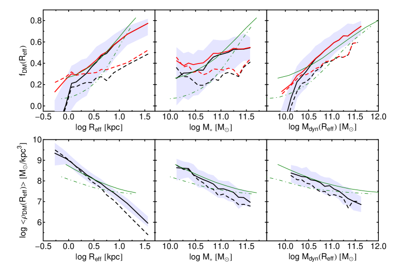
The NFW halos are assumed to follow an average mass-concentration relation, as in Napolitano et al. (2005), while the Sérsic profiles are assumed to follow the $R_{\rm eff}$-$M_{\star}$ and $n-\mbox{$M_{\star}$}$ relations from our data. The virial DM mass is parameterized in terms of a star formation efficiency $\epsilon_{\rm SF}=M_{\star}/(\Omega_{\rm bar}M_{\rm tot})$, where $\Omega_{\rm bar}=0.17$ (Spergel et al. 2007) is the baryon density parameter and $M_{\rm tot}$ is the total mass. We assume that $\epsilon_{\rm SF}$ varies with $M_{\star}$, following the recipes of Conroy & Wechsler (2009), where $\epsilon_{\rm SF}$ decreases from a maximum of $\sim 0.19$ at $\log$ $M_{\star}$$\sim 10.4$ down to $\sim 0.004$ at $\log$ $M_{\star}$$\sim 11.8$. These assumptions allow us to parametrize all toy-model properties (e.g. the central DM fraction) as a function of one single quantity (e.g. $R_{\rm eff}$, $M_{\star}$, or $M_{dyn}$). In Fig. 11, we compare the observed correlations of DM fraction (upper panels) and density (lower panels) with $R_{\rm eff}$, $M_{\star}$, $M_{dyn}$ (from left to right in the Figure), to the toy-models’ predictions, where solid and dashed green curves correspond to AC-NFW and NFW models, respectively. Despite some differences in the trends, we find qualitative agreement between the SIS-based observational results and the toy-models, as the latter occupy a region similar to that of the data in each diagram. On the other hand, adopting an extreme const-${\tt M/L}$ model would produce disagreement between data and theory, which predicts more DM on scales of $\sim$ 10 kpc and beyond.

Figure 12: Comparison of the $f_{\rm DM}$–$M_{\star}$ relation to the predictions of cosmological simulations. The black and red curves, as well as the grey shaded region, are the same as in previous Figures. Red and blue dots correspond to simulated brightest cluster galaxies from Ruszkowski & Springel (2009), for contracted and uncontracted models, respectively. Black dots and open squares are the results of hydrodynamical simulations of O$\rm\tilde{n}$orbe et al. (2007), adopting high and low gas-to-stars conversion efficiency, respectively.

In more detail, uncontracted (i.e. NFW) models predict on average smaller $f_{\rm DM}$ than contracted models (NRT10; T+10). Both sets of toy-models give similar $f_{\rm DM}$  and $\langle\rho_{\rm DM}\rangle$  predictions at high mass ($R_{\rm eff}$), while they deviate more from each other at lower mass ($R_{\rm eff}$), with differences up to $\Delta\mbox{$f_{\rm DM}$}\sim 0.2$ and $\Delta\log\mbox{$\langle\rho_{\rm DM}\rangle$}\sim 0.5\,\rm\mbox{$M_{\odot}$}$ kpc^-3.

The AC model matches the observations well over a broad range of galaxy sizes and masses, which is remarkable since there was no fitting or fine-tuning involved. The NFW model fares less well, particularly for galaxies with small masses and sizes. As discussed in Section 3.4, the apparent implication is that the central DM profiles have density cusps that are steeper than in an NFW profile, and are broadly consistent with adiabatically-contracted NFW profiles (see also NRT10; T+10). Such conclusions will depend on the modelling ingredients, such as the IMF adopted, the $\epsilon_{\rm SF}$ vs $M_{\star}$ relation etc., which it is outside the scope of this paper to examine in detail. Here we can only remark that one way to fix these discrepancies is to allow the $\epsilon_{\rm SF}$ to grow with mass in contrast to the Conroy & Wechsler (2009) predictions.

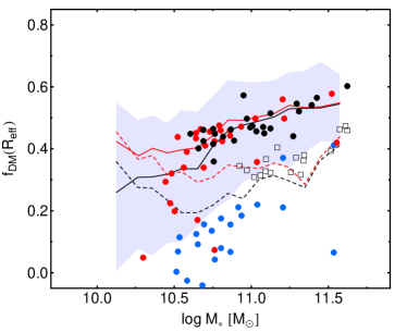
In Fig. 12 we compare our $f_{\rm DM}$–$M_{\star}$ relation with the results of two sets of cosmological simulations: (1) simulated brightest cluster galaxies from Ruszkowski & Springel (2009), using uncontracted and contracted DM models (blue and red dots, respectively); and (2) hydrodynamical simulations from O$\rm\tilde{n}$orbe et al. (2007, hereafter ODS07), for the cases where the authors adopted either a high (black dots) or low (black empty squares) gas-to-stars conversion efficiency.

We find that contracted models are in excellent agreement with the observed ${\tt SIS}$-based $f_{\rm DM}$ values, while uncontracted models produce results closer to const-${\tt M/L}$ $f_{\rm DM}$ estimates, which is qualitatively consistent with our toy-model results. The ${\tt SIS}$ $f_{\rm DM}$–$M_{\star}$  relation is also remarkably consistent with the simulations of ODS07, in the case of high conversion efficiency. On the other hand, const-${\tt M/L}$ $f_{\rm DM}$’s are more consistent to the predictions of models with low conversion efficiency. This is due to the fact that the low efficiency simulations of ODS07 are those producing lower $f_{\rm DM}$’s. In fact, as noticed by the authors (see their Sec. 6.2), adopting a lower conversion efficiency yields lower $R_{\rm eff}$ values, which enclose a smaller portion of a galaxy DM halo, implying lower $f_{\rm DM}$ values. Finally, one should notice that whilst our average $f_{\rm DM}$–$M_{\star}$  relation is fully consistent with that of ODS07, the measured scatter around it is significantly larger than that of the simulations. This might be due to measurement errors, as well as the effect of some other parameter which is not taken into account by simulations (e.g. galaxy stellar populations). Moreover, consistently with the results in Fig. 11, it is encouraging that our $R_{\rm eff}$-$M_{\star}$ relation is broadly consistent with the relation predicted by ODS07 for high efficiency models.

8 Conclusions

We have discussed the central DM content of massive, nearby ($z<0.1$) ETGs, using high quality data from the SPIDER survey, including stellar masses estimated from optical- to NIR-photometry. Using the Jeans equations, we model each galaxy to estimate its dynamical mass, $M_{\rm dyn}$, within 1 $R_{\rm eff}$ in the $K$-band. We have adopted a ${\tt SIS}$ and, as a comparison, a non-homologous const-${\tt M/L}$  model for the total mass profile, in order to investigate the systematics induced by different assumptions for the mass profile. The recovered DM fraction, $f_{\rm DM}$, or equivalently the ratio $\mbox{$M_{\rm dyn}$}/\mbox{$M_{\star}$}$ and the average densities, $\langle\rho_{\rm DM}\rangle$, have been analyzed as a function of structural parameters and different mass proxies, comparing results with predictions of both toy-models and cosmological simulations. The main results are the following:

• For a Chabrier IMF we find that only small fractions ($\sim 12$ and $24\%$ for the ${\tt SIS}$  and const-${\tt M/L}$, respectively) of galaxies have negative DM fractions, while the fractions increase to $\sim 55$ and $78\%$ when a Salpeter IMF is adopted. Thus, under the assumptions that the total mass profiles are well described by a ${\tt SIS}$ or a const-${\tt M/L}$ and the IMF is the same for all galaxies, our data favour a Chabrier (or a Kroupa 2001) IMF, in agreement with, e.g., Cappellari et al. 2006. On the other hand, relaxing the assumption of a universal IMF, for the most massive galaxies in our sample (with mass comparable to the most massive early-type gravitational lenses in the SLACS survey) a Salpeter IMF is consistent with observations (Treu et al. 2010; Auger et al. 2010a). We remark that, at low mass, a Chabrier IMF is also preferred for late-type galaxies (Sonnenfeld et al. 2011; Brewer et al. 2012), and a Salpeter IMF is ruled out for ETGs, compared to a Chabrier IMF, based on lensing and stellar population data (Ferreras, Saha, Burles, 2008; Ferreras et al., 2010).

• DM fractions and densities are, on average, higher when an ${\tt SIS}$  is adopted, when compared with the results using const-${\tt M/L}$ profile. This result is also confirmed by the determinations of the virial coefficient in Eq. (1), $K$, where, on average, $K_{\rm SIS}>K_{\rm M/L}$.

• The DM fraction is a steeply increasing function of $R_{\rm eff}$, Sérsic index, $\sigma$, $M_{\star}$  and $M_{\rm dyn}$, confirming previous findings (Padmanabhan et al. 2004; Cappellari et al. 2006; Hyde & Bernardi 2009a; T+09; Auger et al. 2010b; Cardone & Tortora 2010). Galaxies with denser stellar cores have also lower $f_{\rm DM}$  values. The assumption of a non-homologous const-${\tt M/L}$ profile yields weaker trends. The mass dependencies may provide important clues to the FP tilt. Assuming that central DM trends can be combined with the virial theorem equation, the ${\tt SIS}$ results point to a dominant role of DM. If a non homologous const-${\tt M/L}$ profile is assumed, then almost all the tilt would be due to a non-homology. We have also verified that these results are qualitatively consistent with our previous determinations (T+09 and NRT10).

• Similarly, the central average DM densities are decreasing functions of $R_{\rm eff}$, $n$ and masses. Steeper trends are found when a const-${\tt M/L}$  profile is adopted. In particular, $\mbox{$\langle\rho_{\rm DM}\rangle$}\propto\mbox{$R_{\rm eff}$}^{-1.8}$ and $\mbox{$R_{\rm eff}$}^{-2.2}$ for the ${\tt SIS}$ and const-${\tt M/L}$ respectively, due to the steeper DM density profile for const-${\tt M/L}$ at $R_{\rm eff}$.

• We have compared our results with predictions from $\Lambda$CDM toy-models, finding good qualitative agreement. As in NRT10, we have found that when a Chabrier (or Kroupa) IMF is adopted, a contracted NFW is preferred, while a bottom-heavy IMF like Salpeter would be more consistent with an uncontracted NFW (see, e.g. Cardone & Tortora 2010; NRT10; Treu et al. 2010).

• The role of the environment has been investigated after classifying the galaxies in the field and in groups, and in the latter, centrals have also been examined explicitly. We find no difference in the estimated $f_{\rm DM}$ between field and group galaxies, and only slight differences between centrals and non-centrals. This result is possibly due to an increased role of mergers for the central galaxies.

We have finally shown that a very tight relationship similar to the FP exists between DM fraction, velocity dispersion and size. We have determined the best fitted parameters in Eq. (2) and have inferred that DM might be the dominant driver of FP tilt, at least when a ${\tt SIS}$ is adopted, and under the assumption that central DM trends can be combined with the virial theorem expectation. In a forthcoming paper we will discuss the results introduced here in terms of the stellar population parameters derived from the fitting of spectra, by means of different synthetic prescriptions. In particular, within the general framework introduced in NRT10 and T+10, we will investigate correlations with stellar populations parameters such as age, metallicity, and alpha-enhancement. With further comparisons to simulations, these correlations may be used to constrain the evolution of stars and DM in local galaxies, and to point the way to similar analyses at higher redshifts.

Appendix A Structural parameters and magnitude

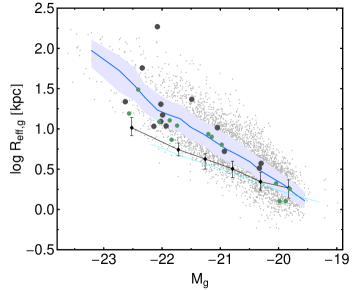
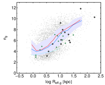
Structural parameters of ETGs, such as the effective radius, $R_{\rm eff}$, are known to be significantly affected by the method (e.g. 1D vs. 2D fitting of the light distribution) and profile shape (e.g. de Vaucouleurs vs. Sérsic law) used to derive them (e.g. Kelson et al. 2000). While such differences do not affect the FP relation of ETGs, because of the correlated variation of $R_{\rm eff}$ and the mean surface brightness therein, $\langle\!\mu\!\rangle_{e}$, they can affect other correlations among structural parameters and luminosity (mass), and hence the correlations with DM fractions (densities). For instance, in Sec. 3.2 we have shown that the $f_{\rm DM}$ correlations presented in the present study are somewhat steeper than those we previously derived in T+09, based on a different sample of ETGs, from Prugniel & Simien (1996, hereafter PS96). We address this issue in Fig. 13, where we compare our $g$-band luminosity–size relation to that of the PS96 $B$-band sample analyzed by T+09. For the sake of completeness, in the same plot we include our $g$-band Sérsic index–size relation, and compare both relations to the $g$-band data from Ferrarese et al. (2006) and Kormendy et al. (2009). Notice that the effective parameters of the PS96 sample are based on de Voucouleurs (rather than Sérsic) galaxy profile fits, hence no comparison to our Sérsic $n$–size relation is possible. We refer the reader to previous papers of the series (Papers I, II) for a detailed comparison of correlations among structural parameters from the SPIDER survey and SDSS pipeline. The present sample of ETGs exhibits a steeper luminosity–size relation than that of the T+09 sample. This is explained by the fact that fitting a high-$n$ galaxy with a de Vaucouleurs profile gives a systematically smaller $R_{\rm eff}$ value, hence flattening the luminosity–size relation (e.g. Graham & Worley 2008). Indeed, this explains why our $f_{\rm DM}$–$R_{\rm eff}$ relation is steeper than that of T+09 (see Fig. 5), as a smaller $R_{\rm eff}$ encloses a smaller portion of the DM halo (implying lower $f_{\rm DM}$ estimates). On the other hand, the correlations among structural parameters for the present sample are in better agreement with those of Ferrarese et al. (2006) and Kormendy et al. (2009). We remark that since significant differences in the $f_{\rm DM}$  correlations exist when analyzing different samples of ETGs (i.e. different sets of structural parameters), it is of paramount importance to compare different samples of galaxies (e.g. different environments) based on a homogeneous set of measurements, as the one used here.

Figure 13: $\mbox{$R_{\rm eff}$}-M_{g}$ (left) and $n_{g}-\mbox{$R_{\rm eff}$}$ (right) correlations. The small grey points are the datapoints in our sample, while the blue lines and shaded regions are the medians and $25-75$ per cent scatter. The red line in the right plot is for the $r$-band data. Large grey points are for bright galaxies in Kormendy et al. (2009). Black points with error bars are the $B$-band results from T+09 (using the sample in Prugniel & Simien (1996)), while the cyan lines show the results using NYU-VAGC data (Blanton et al. 2005), and the green points are the datapoints for the Virgo sample in Ferrarese et al. (2006). Suitable conversion factors are adopted to convert $r$-, $B$- or $V$-band data into $g$-band, and the data have been converted to our adopted cosmology.

Appendix B Dynamical mass procedure

Our basic approach to estimating the DM content of ETGs is the same as in T+09. For each galaxy, we first de-project the corresponding Sérsic (1968) light profile, assuming spherical symmetry. This gives the de-projected luminosity profile, $j_{*}(r)$, where $r$ is the spatial distance to the centre of the galaxy. Using a Sérsic model here has the main advantage of taking into account the non-homology of the stellar matter distribution of ETGs (see, e.g., Caon, Capaccioli & D’Onofrio 1993 and Prugniel & Simien 1997). We also assume some simplified functional form for the dynamical mass profile, $M(r)$, i.e. either a const-${\tt M/L}$ profile, $M(r)=\Upsilon_{0}\,L(r)$, or a SIS model, where $M(r)\propto\sigma_{\rm SIS}^{2}r$ (see Sec. 2). Assuming spherical symmetry and no rotation, we write the Jeans equation as:

$${{\rm d}(j_{*}\sigma_{r}^{2})\over{\rm d}r}+2\,{\beta(r)\over r}\,j_{*}\sigma_{r}^{2}=-j_{*}(r)\,\frac{GM(r)}{r^{2}}\ ,$$ (7)

where $\beta=1-\sigma_{t}^{2}/\sigma_{r}^{2}$ is the anisotropy. Under the hypothesis of isotropy (i.e., $\beta=0$), Eq. (7) simplifies to

$$\sigma_{r}^{2}(r)=\frac{1}{j_{*}(r)}\int_{r}^{\infty}j_{*}\frac{GM}{s^{2}}{\rm d}s\ .$$ (8)

In order to fit the given mass to the data, we project this equation in 2D, obtaining the line-of-sight velocity dispersion:

$$\sigma_{\rm los}^{2}(R)=\frac{2}{I(R)}\,\int_{R}^{\infty}\frac{j_{*}\sigma_{r}^{2}\,r\,{\rm d}r}{\sqrt{r^{2}\!-\!R^{2}}},$$ (9)

where

$$I(R)=2\,\int_{R}^{\infty}\frac{j_{*}\,r}{\sqrt{r^{2}\!-\!R^{2}}}{\rm d}r$$ (10)

is the projected surface brightness profile. We integrate $\sigma_{\rm los}$ within a fixed aperture $R_{\rm Ap}$ (i.e. the SDSS fibre aperture) to obtain the aperture velocity dispersion, $\sigma_{\rm Ap}$:

$$\sigma_{\rm Ap}^{2}(R_{\rm Ap})=\frac{1}{L(R_{\rm Ap})}\int_{0}^{R_{\rm Ap}}2\pi\,S\,I(S)\,\sigma_{\rm los}^{2}(S)\,{\rm d}S\ ,$$ (11)

where $L(R)=\int_{0}^{R}2\pi SI(S)\,{\rm d}S$ is the luminosity within the projected radius $R$. To avoid lengthy calculations, we have adopted the compact formulae for $\sigma_{\rm Ap}$ calculated in Mamon & Łokas (2005a) and Mamon & Łokas (2006) (see Mamon & Łokas (2005b) for the anisotropic case).

Finally, we fit the model $\sigma_{\rm Ap}$ to the observed $\sigma_{spec}$, by varying the free parameters in Eq. (8)  (i.e. either $\sigma_{\rm SIS}$ or $\Upsilon_{0}$) until the desired matching is achieved. The resulting best-fit mass profile provides the dynamical (spherical) mass-to-light ratio within $R_{\rm eff}$, $\Upsilon_{\rm dyn}$ (which coincides with $\Upsilon_{0}$ in the case of a const-${\tt M/L}$ model), and mass $M_{\rm dyn}$. Finally, as we have shown in Sec. 3.1 we notice that a non null radial anisotropy (i.e. $\beta>0$) decreases the $M_{\rm dyn}$, lowering the DM fractions (see text for further details).

References

- Abazajian et al. (2003) Abazajian K.N. et al., 2003, AJ, 126, 2081
- Abazajian et al. (2009) Abazajian K.N., Adelman-McCarthy, J.K., Agüeros, M.A., et al., 2009, ApJS, 182, 543
- Adelman-McCarthy et al. (2008) Adelman-McCarthy, J.K., Agüeros, M.A., Allam, S.S., et al., 2008, ApJS, 175, 297
- Auger et al. (2010a) Auger M. W., Treu T., Gavazzi R., Bolton A. S., Koopmans L. V. E., Marshall P. J. 2010, ApJ, 721, L163
- Auger et al. (2010b) Auger, M. W., Treu, T., Bolton, A. S., Gavazzi, R., Koopmans, L. V. E., Marshall, P. J., Moustakas, L. A., Burles, S. 2010, ApJ, 724, 511
- Barnabè et al. (2011) Barnabè M., Czoske O., Koopmans L. V. E., Treu T., Bolton A. S. 2011, MNRAS, 415, 2215
- Benson et al. (2000) Benson, A.J., Cole, S., Frenk, C.S., Baugh, C.M., Lacey, C.G., 2000, MNRAS, 311, 793
- Berlind et al. (2006) Berlind, A.A., Frieman, J., Weinberg, D.H., et al., 2006, ApJS, 167, 1
- Bernardi et al. (2003a) Bernardi, M., Sheth, R.K., Annis, J., et al., 2003a, AJ, 125, 1817
- Bernardi et al. (2003b) Bernardi M. et al., 2003b, AJ, 125, 1849
- Bernardi et al. (2006) Bernardi, M., et al. 2006, AJ, 131, 1288 (B06)
- Bertin et al. (2002) Bertin G., Ciotti L., Del Principe M., 2002, A&A, 386, 149
- Blanton et al. (2005) Blanton M. R., Lupton R. H., Schlegel D. J., Strauss M. A., Brinkmann J., Fukugita M., Loveday J., 2005, ApJ, 631, 208
- Bolton et al. (2008) Bolton A. S., Burles S., Koopmans L. V. E., Treu T., Gavazzi R., Moustakas L. A., Wayth R., Schlegel D. J., 2008, ApJ, 682, 964
- Boyarsky et al. (2009) Boyarsky, A., Ruchayskiy, O., Iakubovskyi, D., Macciò, A.V., Malyshev, D. 2009a, arXiv : 0911.1774
- Brewer et al. (2012) Brewer B.J. et al. 2012, AxXiv:1201.1677
- Bruzual & Charlot (2003) Bruzual, A. G. & Charlot, S. 2003, MNRAS, 344, 1000
- Bruzual (2007) Bruzual, A. G. 2007, in IAU Symposium, Vol. 241, IAU Symposium, ed. A. Vazdekis & R. F. Peletier, 125-132
- Busarello et al. (1997) Busarello, G., Capaccioli, M., Capozziello, S., Longo, G., & Puddu, E. 1997, A&A, 320, 415
- Calzetti et al. (2000) Calzetti D., Armus L., Bohlin R. C., Kinney A. L., Koornneef J. & Storchi-Bergmann T. 2000, ApJ, 533, 682
- Caon, Capaccioli & D’Onofrio (1993) Caon, N., Capaccioli, M. & D’Onofrio, M. 1993, MNRAS, 265, 1013
- Cappellari et al. (2006) Cappellari, M. et al. 2006, MNRAS, 366, 1126 (C+06)
- Cappellari et al. (2007) Cappellari M. et al., 2007, MNRAS, 379, 418
- Cappellari et al. (2012) Cappellari, M., McDermid, R. M., Alatalo, K., et al. 2012, Nature, 484, 485
- Cardelli et al. (1989) Cardelli J. A., Clayton G. C. & Mathis J. S. 1989, ApJ, 345, 245
- Cardone et al. (2009) Cardone V. F., Tortora C., Molinaro R., Salzano V. 2009, A&A, 504, 769
- Cardone & Tortora (2010) Cardone V. F. & Tortora C. 2010, MNRAS, 409, 1570
- Cardone et al. (2011) Cardone V.F., Angus G., Diaferio A., Tortora C., Molinaro R. 2011, MNRAS, 412, 2617
- Chabrier (2001) Chabrier, G. 2001, ApJ, 554, 1274
- Charlot & Fall (2000) Charlot S. & Fall S. M. 2000, ApJ, 539, 718
- Cid Fernandes et al. (2005) Cid Fernandes, R., González Delgado, R.M., Storchi-Bergmann, T., Martins, L.P., Schmitt, H., 2005, MNRAS, 356, 270
- Ciotti et al. (1996) Ciotti, L., Lanzoni, B., & Renzini, A. 1996, MNRAS, 282, 1
- Conroy & Wechsler (2009) Conroy, C., Wechsler, R. H. 2009, ApJ, 696, 620
- Cooper et al. (2010) Cooper, M.C., Gallazzi, A., Newman, J.A., Yan, R., 2010, MNRAS, 402, 1942
- Deason et al. (2012) Deason, A. J., Belokurov, V., Evans, N. W., & McCarthy, I. G. 2012, ApJ, 748, 2
- Dekel et al. (2005) Dekel, A., Stoehr, F., Mamon, G. A., et al. 2005, Nature, 437, 707
- Donato et al. (2009) Donato F. et al., 2009, MNRAS, 397, 1169
- D’Onofrio et al. (2006) D’Onofrio M., Valentinuzzi T., Secco L., Caimmi R., & Bindoni D. 2006, New Astronomy Review, 50, 447
- D’Onofrio et al. (2008) D’Onofrio M. et al. 2008, ApJ, 685, 875 3
- Douglas et al. (2007) Douglas N. G. et al. 2007, ApJ, 664, 257
- Djorgovski & Davis (1987) Djorgovski, S. & Davis, M. 1987, ApJ, 313, 59
- Dressler et al. (1987) Dressler, A., Lynden-Bell, D., Burstein, D., Davies, R. L., Faber, S. M., Terlevich, R., Wegner, G. 1987, ApJ, 313, 42
- Dutton et al. (2012) Dutton, A. A., Macciò, A. V., Mendel, J. T., & Simard, L. 2012, MNRAS, submitted, arXiv:1204.2825
- Eke et al. (2004) Eke, V., et al. (2dF team), 2004, MNRAS, 348, 866
- Faber & Jackson (1976) Faber, S. M. & Jackson, R. E. 1976, ApJ, 204, 668F
- Faure et al. (2011) Faure C. et al. 2011, A&A, 529, 72
- Ferrarese et al. (2006) Ferrarese L. et al. 2006, ApJS, 164, 334
- Ferreras, Saha, Williams (2005) Ferreras, I., Saha, P., Williams, L.L.R., 2005, ApJ, 623, L5
- Ferreras, Saha, Burles (2008) Ferreras, I., Saha, P., Burles, S., 2008, MNRAS, 383, 857
- Ferreras et al. (2010) Ferreras, I., et al., 2010, MNRAS, 409, L30
- Fioc & Rocca-Volmerange (1997) Fioc M. & Rocca-Volmerange B. 1997, A&A, 326, 950
- Forbes et al. (2008) Forbes D. A., Lasky P., Graham A. W., & Spitler L. 2008, MNRAS, 389, 1924
- Gallazzi et al. (2006) Gallazzi A., Charlot S., Brinchmann J., White S. D. M., 2006, MNRAS, 370, 1106
- Gavazzi et al. (2007) Gavazzi, R., Treu, T., Rhodes, J. D., Koopmans, L. V. E., Bolton, A. S., Burles, S., Massey, R. J., & Moustakas, L. A. 2007, ApJ, 667, 176
- Gentile et al. (2009) Gentile, G., Famaey, B., Zhao, H.S., Salucci, P. 2009, Nature, 461, 627
- Gerhard et al. (2001) Gerhard O., Kronawitter A., Saglia R., Bender R., 2001, AJ, 121, 1936
- Ghigna et al. (1998) Ghigna S. et al. 1998, MNRAS, 300, 146
- Gnedin et al. (2004) Gnedin O. Y., Kravtsov A. V., Klypin A. A. & Nagai D. 2004, ApJ, 616, 16
- Graham & Colless (1997) Graham, A., & Colless, M. 1997, MNRAS, 287, 221
- Graham & Worley (2008) Graham, A. W., & Worley, C. C. 2008, MNRAS, 388, 1708
- Graves (2009) Graves G. J. 2009, Ph.D. Thesis, University of California, Santa Cruz
- Graves & Faber (2010) Graves, G. J., Faber, S. M. 2010, ApJ, 717, 803
- Grillo (2010) Grillo, C. 2010, ApJ, 722, 779
- Hyde & Bernardi (2009a) Hyde J. B. & Bernardi M. 2009a, MNRAS, 394, 1978
- Hyde & Bernardi (2009b) Hyde J. B. & Bernardi M. 2009b, MNRAS, 396, 1171
- Jrgensen et al. (1995) Jrgensen, I., Franx, M., Kjrgaard, P. 1995, MNRAS, 273, 1097
- Jrgensen et al. (1996) Jrgensen, I., Franx, M., Kjrgaard, P. 1996, MNRAS, 280, 167
- Kelson et al. (2000) Kelson, D.D., Illingworth, G.D., van Dokkum, P.G., Franx, M., 2000, ApJ, 531, 137
- Kochanek (1991) Kochanek, C. S. 1991, ApJ, 373, 354
- Koopmans et al. (2006) Koopmans, L. V. E., Treu, T., Bolton, A. S., Burles, S., Moustakas, L. A. 2006, ApJ, 649, 599
- Kormendy (1977) Kormendy, J. 1977, ApJ, 218, 333
- Kormendy et al. (2009) Kormendy J., Fisher D. B., Cornell M. E., Bender R. 2009, ApJS, 182, 216
- Kroupa (2001) Kroupa P., 2001, MNRAS, 322, 231
- Ilbert et al. (2006) Ilbert, O. et al. 2006, A&A, 457, 841
- La Barbera et al. (2008a) La Barbera, F., de Carvalho, R.R., Kohl-Moreira, J.L., Gal, R.R., Soares-Santos, M., Capaccioli, M., Santos, R., Sant’anna, N., 2008a, PASP, 120, 681
- La Barbera et al. (2008b) La Barbera, F., Busarello, G., Merluzzi, P., de la Rosa, I.G., Coppola, G., Haines, C.P., 2008b, ApJ, 689, 913
- La Barbera & de Carvalho (2009) La Barbera, F., de Carvalho, R.R., 2009, ApJL, 699, 76
- La Barbera et al. (2010a) La Barbera F., de Carvalho R. R., de La Rosa I. G., Lopes P. A. A., Kohl-Moreira J. L., Capelato, H. V. 2010a, MNRAS, 408, 1313 (Paper I)
- La Barbera et al. (2010b) La Barbera F., de Carvalho R. R., de La Rosa I. G., Lopes P. A. A. 2010b, MNRAS, 408, 1335 (Paper II)
- La Barbera et al. (2010c) La Barbera F., Lopes P. A. A., de Carvalho R. R., de La Rosa I. G., Berlind A. A. 2010c, MNRAS, 408, 1361 (Paper III)
- La Barbera et al. (2010d) La Barbera F., De Carvalho R. R., De La Rosa I. G., Gal R. R., Swindle R., Lopes P. A. A. 2010d, AJ, 140, 1528 (Paper IV)
- Leier et al. (2011) Leier, D., Ferreras, I., Saha, P., Falco, E.E., 2011, ApJ, 740, 97
- Lopes et al. (2009a) Lopes, P.A.A., de Carvalho, R.R., Kohl-Moreira, J.L., Jones, C., 2009, MNRAS, 392, 135
- Lubini et al. (2011) Lubini, M., Tortora, C., Näf, J., Jetzer, Ph., Capozziello, S. 2011, EPJC, 71, 1834
- Madau (1995) Madau, P. 1995, ApJ, 441, 18
- Mamon & Łokas (2005a) Mamon G.A. & Łokas E.L., 2005a, MNRAS, 362, 95
- Mamon & Łokas (2005b) Mamon G.A. & Łokas E.L., 2005b, MNRAS, 363, 705
- Mamon & Łokas (2006) Mamon G.A. & Łokas E.L., 2006, MNRAS, 370 1581
- Marinoni & Hudson (2002) Marinoni C. & Hudson M.J. 2002, ApJ, 569, 101
- More et al. (2011) More A., Jahnke K., More S., Gallazzi A., Bell E. F., Barden M., Huler, B. 2011, ApJ, 734, 69
- Napolitano et al. (2005) Napolitano, N. R., Capaccioli, M., Romanowsky, A. J., Douglas, N. G., Merrifield, M. R., Kuijken, K., Arnaboldi, M., Gerhard, O., Freeman, K. C. 2005, MNRAS, 357, 691 (N+05)
- Napolitano, Romanowsky & Tortora (2010) Napolitano N. R., Romanowsky A. J. & Tortora, C. 2010, MNRAS, 405, 2351 (NRT10)
- Napolitano et al. (2012) Napolitano, N. R., Capozziello, S., Romanowsky, A.J., Capaccioli, M., & Tortora, C. 2012, ApJ, 748, 87
- Navarro, Frenk & White (1997) Navarro, J. F., Frenk, C. S., & White, S. D. M. 1997, ApJ, 490, 493 (NFW)
- Oorbe et al. (2007) Oorbe, J., Domínguez-Tenreiro, R. Sáiz A., Serna A.,2007, MNRAS, 376, 39
- Padmanabhan et al. (2004) Padmanabhan, N. et al. 2004, NewA, 9, 329P
- Pahre et al. (1995) Pahre, M. A., Djorgovski, S. G., & de Carvalho, R. R. 1995, ApJ, 453, L17
- Prugniel & Simien (1996) Prugniel, Ph. & Simien F. 1996, A&A, 309, 749
- Prugniel & Simien (1997) Prugniel, Ph. & Simien F. 1997, A&A, 321, 111
- Richtler et al. (2011) Richtler, T., Famaey, B., Gentile, G., & Schuberth, Y. 2011, A&A, 531, A100
- Romanowsky et al. (2003) Romanowsky, A. J., Douglas, N. G., Arnaboldi, M., et al. 2003, Science, 301, 1696
- Ruszkowski & Springel (2009) Ruszkowski M. & Springel V. 2009, ApJ, 696, 1094
- Salpeter (1955) Salpeter, E.E. 1955 ApJ, 121, 161
- Schulz et al. (2010) Schulz A. E., Mandelbaum R., Padmanabhan N., 2010, MNRAS, 408, 1463
- Shankar & Bernardi (2009) Shankar, F., & Bernardi, M. 2009, MNRAS, 396, L76
- Shen et al. (2003) Shen, S., Mo, H.J., White, S.D.M., Blanton, M.R., Kauffmann, G., Voges, W., Brinkmann, J., Csabai, I. 2003, MNRAS, 343, 978
- Sérsic (1968) Sérsic, J. L. 1968, Atlas de Galaxies Australes, Observatorio Astronomico de Cordoba
- Sonnenfeld et al. (2011) Sonnenfeld A., Treu T., Gavazzi R., Marshall P.J., Auger M.W., Suyu S. H., Koopmans L. V. E., Bolton A. S. 2011, arXiv:1111.4215
- Spergel et al. (2007) Spergel, D. N., et al. 2007, ApJS, 170, 377
- Swindle et al. (2011) Swindle R., Gal R. R., La Barbera F., de Carvalho R. R. 2011, AJ, 142, 118 (Paper V)
- Thomas et al. (2005) Thomas, D., et al. 2005, ApJ, 621, 673
- Thomas et al. (2009) Thomas J., Saglia R. P., Bender R., Thomas D., Gebhardt K., Magorrian J., Corsini E. M., Wegner G., 2009, ApJ, 691, 770
- Tortora et al. (2009) Tortora C. et al. 2009, MNRAS, 396, 1132 (T+09)
- Tortora et al. (2010) Tortora C., Napolitano N. R., Romanowsky A. J., Jetzer P. 2010, ApJ, 721, 1 (T+10)
- Treu et al. (2010) Treu, T., Auger, M. W., Koopmans, L. V. E., Gavazzi, R., Marshall, P. J. & Bolton, A. S. 2010, ApJ, 709, 119
- Trujillo, Burkert & Bell (2004) Trujillo, I., Burkert, A. & Bell, E.F. 2004, ApJ, 600, L39
- van den Bosch et al. (2007) van den Bosch, F.C. et al. 2007, MNRAS, 376, 841
- van Dokkum & Conroy (2011) van Dokkum P. G. & Conroy C. 2011, ApJ, 735, 13
- Walker et al. (2009) Walker, M. G., Mateo, M., Olszewski, E. W., et al. 2009, ApJ, 704, 1274
- Wolf et al. (2010) Wolf, J., Martinez, G. D., Bullock, J. S., et al. 2010, MNRAS, 406, 1220
- Yang et al. (2007) Yang, X., Mo, H.J., van den Bosch, F.C., Pasquali, A., Li, C., Barden, M., 2007, ApJ, 671, 153