Double null formulation of the general Vaidya metric

Abstract

We present here the field equations describing a non-stationary spherically symmetric $n$-dimensional charged black hole with varying mass $m(v)$ and/or electric charge $q(v)$, described by a generic charged Vaidya metric with cosmological constant $\Lambda$ in double null coordinates. This formulation of the metric has been shown to be particularly useful for perturbative studies and it was used in some recent works. Here we also discuss some issues related to the apparent and event horizons of the black hole.

1 Introduction

In 1951, P. C. Vaidya presented for the first time a metric to describe the spacetime outside a spherically symmetric star, taking into account the radiation flux emitted by the star [1]. In his work, the mass of the star is no longer considered to be constant and the metric is not static. The situation is described as a spherical mass surrounded by a finite and nonstatic envelope of radiation with radial symmetry.

This metric has been the usual starting point for the study of the quasinormal modes of time dependent black holes [2, 3, 4, 5, 6]. The charged version of the metric is also an usual starting point for the study of many aspects of charged black hole physics [7, 8, 9, 10, 11, 12, 13].

The Vaidya metric has also been used to describe spherically symmetric collapse and the formation of naked singularities [14, 15]. It was also applied to the study of Hawking radiation and the process of black hole evaporation [16, 17, 18, 19], in the stochastic gravity program [20], and in recent numerical relativity investigations [21].

In the study of quasinormal modes, it is useful to write the Vaidya metric in double null coordinates [4, 5, 22]. However, there is no general coordinate transformation from the usual radiation coordinates to double null coordinates [23]. So our purpose with this paper is to present the most general Vaidya metric, $n$-dimensional, with cosmological constant $\Lambda$ and with time dependent mass and electrical charge in these coordinates.

The numerical results are obtained with a generalization of the semi-analytical method used in [24, 25], that allows us to construct the structure of the spacetime from the behavior of the outgoing null geodesics.

The structure of the paper is as follows. In section 2 we present the derivation of the most general Vaidya metric in double-null coordinates. In section 3 we present a discussion on the structure of the spacetime and the numerical results obtained with the semi-analytical method. And finally in section 4 we present our final discussion of the results.

2 The general Vaidya metric in double-null coordinates

The $n$-dimensional Vaidya metric was first discussed in [26]. It can be easily cast in $n$-dimensional radiation coordinates $(v,r,\theta_{1},\dots,\theta_{n-2})$ as done, for instance, in [27]. The $n$-dimensional charged Vaidya metric in radiation coordinates, obtained originally in [8], reads

$$\rmd s^{2}=-\left(1-\frac{2m(v)}{(n-3)r^{n-3}}+\frac{2q^{2}}{(n-2)(n-3)r^{2(n-3)}}\right)\rmd v^{2}+2c\rmd r\rmd v+r^{2}\rmd\Omega^{2}_{n-2},$$ (1)

where $n>3$, $c=\pm 1$, and $\rmd\Omega^{2}_{n-2}$ stands for the metric of the unit $(n-2)$-dimensional sphere, assumed here to be spanned by the angular coordinates $(\theta_{1},\theta_{2},\dots,\theta_{n-2})$,

$$\rmd\Omega^{2}_{n-2}=\sum_{i=1}^{n-2}\left(\prod_{j=1}^{i-1}\sin^{2}\theta_{j}\right)\rmd\theta_{i}^{2}.$$ (2)

For the case of an ingoing radial flow, $c=1$ and $m(v)$ is a monotonically increasing mass function in the advanced time $v$, while $c=-1$ corresponds to an outgoing radial flow, with $m(v)$ being in this case a monotonically decreasing mass function in the retarded time $v$. The constant $q$ corresponds to the total electric charge. In principle, one can also consider time dependent charges $q$ as done, for instance, in [9]. This situation will of course require the presence of charged null fluids and currents, whose realistic nature we do not address here.

It has been known since a long time that the radiation coordinates are defective at the horizon [28], implying that the Vaidya metric (1), with or without electric charge, is not geodesically complete in any dimension. The radiation coordinates are not enough to cover the entire Vaidya spacetime. (The radiation coordinates are defective at horizons where $v^{2}\to\infty$). As can be seen in [28], for a 4-dimensional Vaidya metric with $dm/du<0$ and without electric charge (in the context of ref. [28], a radiating star), the hypersurface $r=2m(\infty)$ at $v=\infty$ in the Vaidya metric is analogous to the Schwarzschild hypersurface $r=2m$ at Schwarzschild’s time coordinate $T=+\infty$ in the Kruskal metric. (See [10] and [29] for further discussions about possible analytical extensions and properties of the horizon of the Vaidya metric in the radiation coordinates).

The cross term $drdv$ introduces extra terms in the hyperbolic equations governing the evolution of physical fields on spacetimes with the metric (1). Typically, the double-null coordinates are far more convenient for QNM analysis. This was the main motivation of the series of works based on Waugh and Lake’s approach [23], where the problem of casting the 4-dimensional Vaidya metric in double-null coordinates was originally addressed. As all previous attempts to construct a general transformation from radiation to double-null coordinates had failed, Waugh and Lake considered the problem of solving Einstein’s equation with spherical symmetry directly in double-null coordinates. The resulting equations, however, are not analytically solvable in general. Waugh and Lake’s work was revisited in [24], where a semi-analytical approach allowing for general mass functions was proposed.

More recently this semi-analytical approach was extended to the case of an $n$-dimensional Vaidya metric with cosmological constant $\Lambda$ [25]. This approach consists in a qualitative study of the null-geodesics, allowing the description of light-cones and revealing many features of the underlying causal structure. It can also be used for more quantitative analyses; indeed, it has already enhanced considerably the accuracy of the quasinormal modes analysis of varying mass black holes [4, 5], and it can also be applied to the study of gravitational collapse[24].

In this section, we extend the approach proposed in [25] and derive the double-null formulation for the most general Vaidya metric: $n$-dimensional, in the presence of a cosmological constant, and with varying electric charge and mass. Only the main results are presented. The reader can get more details on the employed semi-analytical approach in [25] and the references cited therein. We recall that the $n$-dimensional spherically symmetric line element in double-null coordinates $(u,v,\theta_{1},\dots,\theta_{n-2})$ is given by

$$\rmd s^{2}=-2f(u,v)\rmd u\,\rmd v+r^{2}(u,v)\rmd\Omega^{2}_{n-2},$$ (3)

where $f(u,v)$ and $r(u,v)$ are non vanishing smooth functions. The energy-momentum tensor of a unidirectional radial null-fluid in the eikonal approximation in the presence of an electromagnetic field $F_{ab}$ is given by

$$T_{ab}=\frac{1}{8\pi}hk_{a}k_{b}+\frac{1}{4\pi}\left(F_{ac}F^{\phantom{b}c}_{b}-\frac{1}{4}g_{ab}F_{cd}F^{cd}\right),$$ (4)

where $k_{a}$ is a radial null vector and $h(u,v)$ is a smooth function characterizing the null-fluid radial flow. In the double null coordinates $(u,v,\theta_{1},\ldots,\theta_{n-2})$, we can choose either $k^{a}=(1,0,0,\ldots,0)$ (flow along the $u$-direction) or $k^{a}=(0,1,0,\ldots,0)$ (flow along the $v$-direction). Since the $u$ and $v$ directions are unspecified, it is not in fact necessary to consider flows along both directions. We will consider here, without loss of generality, the case of a flow along the $v$-direction, as done in [23].

Maxwell equations are given by

$$\frac{1}{\sqrt{-g}}\partial_{a}\sqrt{-g}F^{ab}=4\pi J^{b},$$ (5a)

$$F_{ab,c}+F_{ca,b}+F_{bc,a}=0\,,$$ (5b)

where, for the metric (3),

$$\sqrt{-g}=fr^{n-2}\prod_{j=1}^{n-3}\left(\sin\theta_{j}\right)^{n-j-2}.$$ (5f)

All geometrical quantities relevant to this work are listed in the appendix of [25]. The equations (5a) have the following static spherically symmetric solution

$$F^{uv}=-F^{vu}=\frac{q}{fr^{n-2}},$$ (5g)

with all other components of the electromagnetic tensor vanishing, where $q$ is a constant which one identifies as the $n$-dimensional electric monopole charge. This case, of course, corresponds to $J^{b}=0$. In order to allow for a time dependent charge $q(v)$, one needs to assume the presence of a current

$$J^{u}=\frac{1}{4\pi}\frac{\dot{q}(v)}{fr^{n-2}},$$ (5h)

(with all other components vanishing) which is obtained from the continuity equation $J^{a}_{\phantom{a};a}=0$, as done, for instance, in [9]. Such a current must naturally appear, as we will see, in the $h(u,v)$ function characterizing the radial flow in the energy momentum tensor (4). We note here that our solution (5g) for $F^{ab}$ with $q(v)$ also consistently satisfies the sourceless Maxwell equations (5b).

Einstein equations with cosmological constant $\Lambda$

$$R_{ab}-\frac{1}{2}g_{ab}R=-\Lambda g_{ab}+8\pi T_{ab}\,,$$ (5i)

imply that, for the energy-momentum tensor (4),

$$R=\frac{2n}{n-2}\Lambda-2\frac{n-4}{n-2}\frac{q^{2}}{r^{2(n-2)}},$$ (5j)

where (5g) was used. The _uu and _vv components of Einstein equations for this case read simply

$$\frac{f_{,u}}{f}-\frac{r_{,uu}}{r_{,u}}=0,$$ (5k)

$$\frac{f_{,v}}{f}-\frac{r_{,vv}}{r_{,v}}=\frac{h}{n-2}\frac{r}{r_{,v}},$$ (5l)

where _,u and _,v denote, respectively, differentiation with respect to $u$ and $v$ as usual. The _uv and ${}_{\theta_{j}\theta_{j}}$ components are, respectively,

$$\frac{f_{,u}f_{,v}}{f^{2}}-\frac{f_{,uv}}{f}-(n-2)\frac{r_{,uv}}{r}=-\frac{2\Lambda}{n-2}f+2\frac{n-3}{n-2}f\frac{q^{2}}{r^{2(n-2)}},$$ (5m)

$$\frac{2}{f}\left(rr_{,uv}+(n-3)r_{,u}r_{,v}\right)+(n-3)=\frac{2\Lambda}{n-2}r^{2}+\frac{2}{n-2}\frac{q^{2}}{r^{2(n-3)}}.$$ (5n)

For $n\neq 3$, differentiating Eq. (5n) with respect to $u$ and then inserting Eq. (5k) leads to

$$\frac{r^{n-2}r_{,uv}}{f}-\frac{2\Lambda}{(n-2)(n-1)}r^{n-1}-\frac{2}{n-2}\frac{q^{2}}{r^{n-3}}=-m,$$ (5o)

(after integration with respect to $u$) where $m(v)$ is an arbitrary integration function that we already known from [25] that can be interpreted as the mass of the solution. The $n=3$ case must be considered separately, in an analogous way as done for $q=0$ in [25], and the most important results are presented in the Appendix. Now, differentiating Eq. (5n) with respect to $v$ and using (5l) and (5o) gives

$$h=-\left(\frac{n-2}{n-3}\right)\frac{f}{r^{n-2}r_{,u}}\left(m_{,v}-\frac{1}{n-2}\frac{(q^{2})_{,v}}{r^{n-3}}\right).$$ (5p)

Eq. (5k) is ready to be integrated

$$f=2Br_{,u}\,,$$ (5q)

where $B(v)$ is another arbitrary (but nonvanishing) integration function. From (5p) and (5q), one has

$$h=-2\left(\frac{n-2}{n-3}\right)\frac{B}{r^{n-2}}\left(m_{,v}-\frac{1}{n-2}\frac{(q^{2})_{,v}}{r^{n-3}}\right).$$ (5r)

Finally, by using (5n) and (5q), Eq. (5o) can be written as

$$r_{,v}=-B\left(1-\frac{2m(v)}{(n-3)r^{n-3}}-\frac{2\Lambda}{(n-2)(n-1)}r^{2}+\frac{2}{(n-2)(n-3)}\frac{q^{2}(v)}{r^{2(n-3)}}\right).$$ (5s)

Note that (5m) and (5q) reproduce (5o). Einstein equations are, therefore, equivalent to the equations (5q), (5r), and (5s), generalizing the previous results of [23], [24] and [25].

As already mentioned, the physical interpretation of the arbitrary integration functions $m(v)$ and $B(v)$ are the same of the $q=0$ case. Transforming from the double-null coordinates back to the radiation coordinates by the coordinate change $(u,v)\rightarrow(r(u,v),v)$, the metric (3) will read

$$\rmd s^{2}=4Br_{,v}\rmd v^{2}-4B\rmd r\rmd v+r^{2}\rmd\Omega^{2}_{n-2},$$ (5t)

where (5q) was explicitly used. Comparing (1) and (5t) and taking (5s) into account, it is clear that with the choice $B=\pm 1/2,$ the function $m(v)$ indeed represents the mass of the $n$-dimensional charged solution. The coordinate transformation leading to (5t) also ensures that the Vaidya metric in radiation coordinates (1) and the double null metric (3) constructed in this paper are (locally) isometric. It is important to stress this fact, given the absence of a Birkhoff theorem for non vacuum spacetimes.

As in the $q=0$ case, the weak energy condition applied for (4) requires, from (5r), that

$$B\left(m_{,v}-\frac{1}{n-2}\frac{(q^{2})_{,v}}{r^{n-3}}\right)<0\,.$$ (5u)

If there are both mass and charge variations, then $m_{,v}$ and $q_{,v}$ cannot be chosen arbitrarily (see [9] for a discussion) and must chosen satisfy the energy condition (5u).

Taking (as mentioned above) $B=\pm\frac{1}{2}$, if we have only mass (or charge) varying with time, the energy condition requires that $m(v)$ (or $q(v)$) be a monotonic function and fixes $B$ in the following way:

$$\textrm{if}\ m_{,v}>0\ (\textrm{or}\ q_{,v}<0)\ \textrm{then}\ B=-\frac{1}{2}\,,$$

$$\textrm{if}\ m_{,v}<0\ (\textrm{or}\ q_{,v}>0)\ \textrm{then}\ B=+\frac{1}{2}\,,$$

where we consider, without loss of generality, $q(v)>0$.

3 The spacetime structure

The problem of constructing a double-null formulation for the general Vaidya metric may be stated as follows: given the mass function $m(v)$, the electric charge function $q(v)$, the cosmological constant $\Lambda$, and the constant $B$, one needs to solve Eq. (5s), obtaining the function $r(u,v)$. Then, $f(u,v)$ and $h(u,v)$ are calculated from (5q) and (5r). The arbitrary function of $u$ appearing in the integration of (5s) must be chosen properly [23], so that $f(u,v)$ given in (5q) is a non-vanishing function. Unfortunately, as stressed previously by Waugh and Lake[23], such a procedure is not analytically solvable in general. In [25], a semi-analytical procedure is introduced to attack the problem of solving Eqs. (5q)-(5s) for the $q=0$ case, generalizing in this way the results of [24] obtained for $n=4$ and $\Lambda=0$.

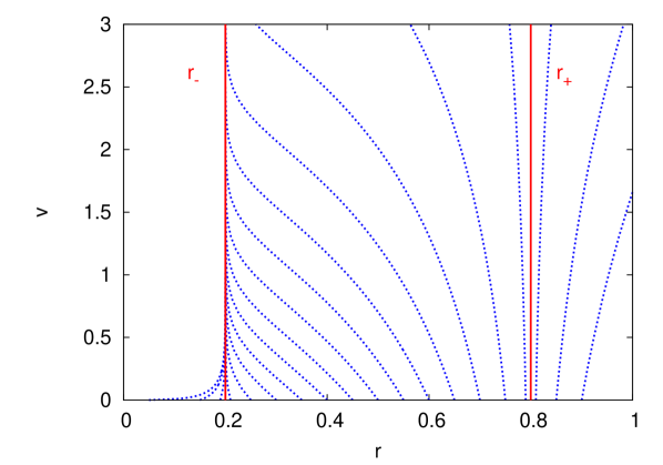
Figure 1: Example of $u$-constant null-geodesics (dotted lines) obtained from Eq. (5s) for the usual Reissner-Nordström case, corresponding to $B=-1/2$, $m=0.5$, $q=0.4$, $n=4$, $\Lambda=0$, and taking $r(u,v=0)=-u/2$. (See [24]). Here $r_{+}$ and $r_{-}$ (solid lines) are defined as usual as $r_{\pm}=m\pm\sqrt{m^{2}-q^{2}}$. In the exterior region ($r>r_{+}$), the constant $u$ null geodesics reach ${\cal I}^{+}$, while in the interior region they are confined, giving origin to the typical black hole causal structure.

The approach, which we will not reproduce here, allows us to qualitatively construct conformal diagrams, identifying horizons and singularities, and also to evaluate specific geometric quantities. The main idea, however, is to solve Eq. (5s) numerically as an initial value in $v$, for constant $u$. In other words, we obtain numerically $r(u,v)$ for $u$ constant, starting with a initial condition

$$r(u,v_{0})=F(u),$$ (5v)

where we must have $F^{\prime}(u)\neq 0$, as can be seen from (5q). In analogy with the flat spacetime case, we choose here $F(u)=-\frac{u}{2}$. Since the lines of constant $u$ (or $v$) are null geodesics for any metric in double-null coordinates, knowing $r(u,v)$ for $u$ constant is enough, for instance, to construct the causal conformal diagrams. Figure (1) depicts a simple example, corresponding to the usual Reissner-Nordström solution.

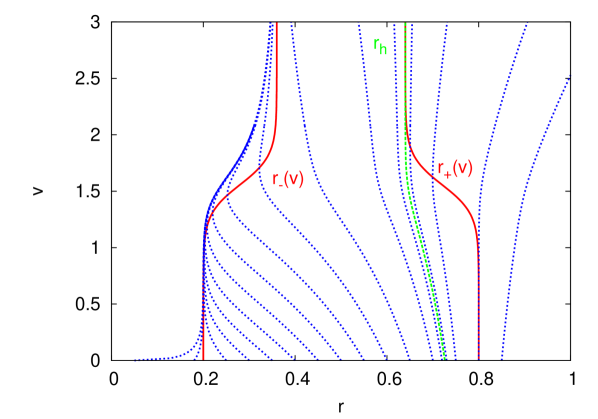
Figure 2: Example of $u$-constant null-geodesics (dotted lines) obtained from Eq. (5s), with the same parameter values used in Figure 1 but now with a time dependent charge function given by $2q(v)=\left(q_{f}+q_{i}\right)+\left(q_{f}-q_{i}\right)\tanh\rho(v-v_{m})$, with $q_{i}=0.4$, $q_{f}=0.48$, $\rho=4.0$ and $v_{m}=1.5$. We can see in this case that the $r_{\pm}$ (solid lines) are no longer constant, and the event horizon $r_{h}$ (dashed line) no longer coincides with $r_{+}$.

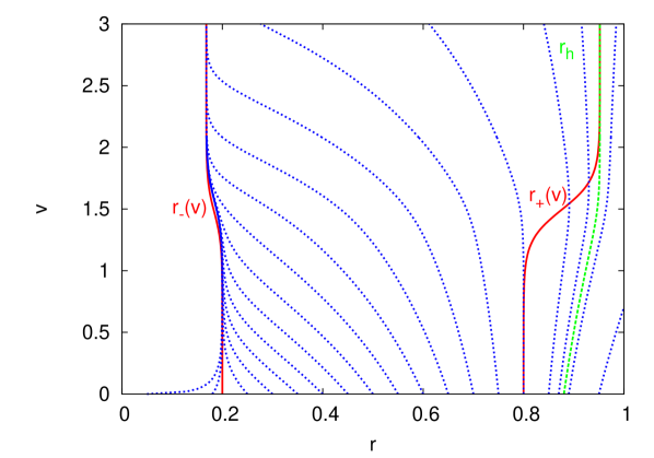
Figure 3: Same as Figure 2, but this time with $q=0.4$ and $2m(v)=\left(m_{f}+m_{i}\right)+\left(m_{f}-m_{i}\right)\tanh\rho(v-v_{m})$, with $m_{i}=0.5$, $m_{f}=0.56$, $\rho=4.0$ and $v_{m}=1.5$.

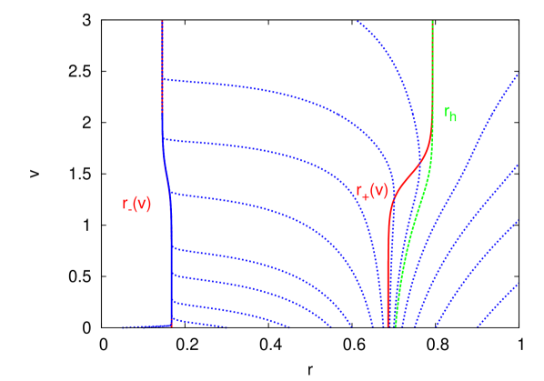
Figure 4: Same as Figure 3, but this time exploring a 5-dimensional solution ($n=5$), with $q=0.2$, $m_{i}=0.5$ and $m_{f}=0.65$. The apparent horizons are now at $r\pm=\left[\frac{1}{2}\left(m\pm\sqrt{m^{2}-\frac{4}{3}q^{2}}\right)\right]^{1/2}$ and therefore we must have $\sqrt{3}m>2q$. The behavior is qualitatively the same as for the $n=4$ case.

Figure 5: Same as Figure 3, but this time allowing a non-zero cosmological constant $\Lambda=0.3$, with $q=0.4$, $m_{i}=0.5$, $m_{f}=0.65$, $\rho=1.0$ and $v_{m}=15$. The striking feature in this case is the existence of three time-dependent apparent horizons $r_{-},r_{+}$ and $r_{c}$, located at the positive roots of Eq. (5s), which is a 4th order polynomial in this case.

Figures 2 and 3 present the behavior of the $u$-constant null-geodesics in two different time dependent cases: increasing charge function $q(v)$ and increasing mass function $m(v)$. Charge and mass variations produce opposite results for the horizons. Also, $r_{-}$ and $r_{+}$ are now time dependent, and the event horizon $r_{h}$ is no longer coincident with the apparent horizon $r_{+}$.

The case presented in Fig. 2 deserves a more detailed analysis. The charge increase is analogous to the mass evaporation studied in [24, 25].

Following our discussion in Section 2, when $q_{,v}>0$ we must have $B=+\frac{1}{2}$, in order to satisfy the weak energy condition (5u). Now there is a subtlety regarding the sign of $B$. We can see from Eq. (5q) that the sign of $f$ depends on the signs of $B$ and $r_{,u}$ (which is of negative sign with our choice of $F(u)$). Therefore, for $B=-\frac{1}{2}$, we have $f>0$ and $\partial_{u}+\partial_{v}$ is timelike and $\partial_{v}-\partial_{u}$ is spacelike. However, for $B=+\frac{1}{2}$, $f$ has the opposite sign and the timelike and spacelike directions are now exchanged.

The transformation $(u,v)\to(v,-u)$ restores the temporal and spatial directions. Under this transformation, Eq. (5s) (with $B=+\frac{1}{2}$) becomes

$$-r_{,u}=-\frac{1}{2}\left(1-\frac{2m(-u)}{(n-3)r^{n-3}}-\frac{2\Lambda}{(n-2)(n-1)}r^{2}+\frac{2}{(n-2)(n-3)}\frac{q^{2}(-u)}{r^{2(n-3)}}\right),$$

which is formally identical to a case with $B=-\frac{1}{2}$, mass function $m(-u)$ and charge function $q(-u)$. Therefore, the transformed equation results in a situation with decreasing charge, that is, a time reversal of the original situation with increasing charge. Stated in a different way, this means that the case with increasing charge and $B=+\frac{1}{2}$ must be interpreted as the time reversal of the case with decreasing charge and $B=-\frac{1}{2}$ (with both cases satisfying the weak energy condition).

However, in order to describe an actual charge increase (equivalent to an evaporation), we need to violate the weak energy condition, since there are no classical processes that can lead to black hole evaporation. In order to do that, we deliberately choose $B=-\frac{1}{2}$ together with $q_{,v}>0$. The weak energy condition is violated, and the resulting evaporation process is shown in Figure 2.

In Figure 4 we show an example of a higher dimensional spacetime with $n=5$. The results are qualitatively the same as for the 4-dimensional cases we presented in Figs. 2 and 3. In Figure 5 we have a qualitatively different behavior, due to the appearance of a cosmological horizon ($\Lambda\neq 0$).

The calculation of the apparent horizons $r\pm(v)$ shown in Figures 1-5 follows the semi-analytic method described in refs. [24, 25]. We can see that the curves defined by the vanishing of the r.h.s of Eq. (5s) always describe the frontier between two regions of the $(v,r)$ plane where the solutions of Eq. (5s) have distinct behaviors. For $r_{,v}<0$, the null geodesics approach the singularity, whereas for $r_{,v}>0$, the null geodesics tend to escape from the singularity.

The determination of the event horizon $r_{h}$ is done numerically by inspection of the initial value $r(u,v_{0})$. The event horizon is found as the last geodesic that escapes towards infinity and does not fall into the singularity. Note that in the case of increasing charge (or, equivalently, decreasing mass) there are null geodesics that escape towards infinity even though they were initially inside the apparent horizon $r_{+}$.

4 Final discussion

We have presented a formulation in double-null coordinates of the most general Vaidya metric: $n$-dimensional, with varying mass and/or charge and cosmological constant $\Lambda$.

By exploring the numerical solutions of Eq. (5s), we were able to highlight some interesting features of the behavior of time-dependent horizons in multiple-horizon spacetimes. The $u$-constant geodesics can be used to track the time dependent event and Cauchy horizons, that no longer coincide with $r_{+}$ and $r_{-}$.

The formulation presented here for the Einstein Eqs. (5q)-(5s) was recently used in a quasinormal mode analysis of the Vaidya metric [22], and provided the framework needed to obtain the quasinormal frequencies with sufficient accuracy to verify their nonstationary behavior.

Appendix

Here we present a short discussion and the results for the Einstein equations (5k)-(5n) for the $n=3$ case, generalizing the discussion of [25]. For $n=3$, Eq. (5k) is still valid and can be integrated to give

$$f=2Br_{,u}\,,$$ (5w)

same as Eq. (5q).

Taking $n=3$, Eq. (5n) reads

$$rr_{,uv}-(\Lambda r^{2}+q^{2})f=0\,,$$ (5x)

and we can use Eq. (5w) to integrate Eq. (5x) and obtain

$$r_{,v}=-B(-m-\Lambda r^{2}-2q^{2}\ln r)\,,$$ (5y)

which is the $n=3$ version of Eq. (5s). Here $m(v)$ is an integration function that has the same interpretation as before, that is, the mass of the solution. Compare (5y) with the charged BTZ black hole [30].

From Eq. (5l) with $n=3$, we have

$$h=\frac{r_{,v}}{r}\frac{f_{,v}}{f}-\frac{r_{,vv}}{r}\,,$$ (5z)

and using Eqs. (5y) and (5w) to get

$$f_{,v}=2B\left(\Lambda r+\frac{q^{2}}{r}\right)f\,,$$ (5aa)

we obtain the $n=3$ version of Eq. (5l):

$$h=-B\left(\frac{m_{,v}}{r}+\frac{4\ln r}{r}qq_{,v}\right)\,.$$ (5ab)

We also note here that the $n=3$ version of Eq. (5m),

$$\frac{f_{,u}f_{,v}}{f^{2}}-\frac{f_{,uv}}{f}-\frac{r_{,uv}}{r}=-2\Lambda f\,,$$ (5ac)

together with Eq. (5w) still reproduce Eq. (5o) with $n=3$.

So finally we can conclude that the Einstein equations (5k)-(5n), which in the $n\geq 4$ case are equivalent to Eqs. (5q)-(5s), are equivalent in the $n=3$ case to Eqs. (5w), (5y) and (5ab).

References

References

- [1] Vaidya P C 1951 Proc. Indian Acad. Sci. A 33 264
- [2] Xue L H, Shen Z X, Wang B and Su R K 2004 Mod. Phys. Lett. A 19 239
- [3] Shao C G, Wang B, Abdalla E and Su R K 2005 Phys. Rev. D 71 044003
- [4] Abdalla E, Chirenti C B M H and Saa A 2006 Phys. Rev. D 74 084029
- [5] Abdalla E, Chirenti C B M H and Saa A 2007 J. High Energy Phys. 0710 086
- [6] He X, Wang B, Wu S F and Lin C Y 2009 Phys. Lett. B 673 156
- [7] Krori K D and Barua J 1974 J. Phys. A: Math. Gen. 7 2125
- [8] Chatterjee S, Bhui B and Banerjee A 1990 J. Math. Phys. 31 2208
- [9] Ori A 1991 Class. Quantum Grav. 8 1559
- [10] Fayos F, Martin-Prats M M and Senovilla J M M 1993 Class. Quantum Grav. 12 2565
- [11] Parikh M K and Wilczek F 1999 Phys. Lett. B 449 24
- [12] Hong S E, Hwang D, Stewart E D and Yeom D 2010 Class. Quantum Grav. 27 045014
- [13] Hwang D and Yeom D 2011 Phys. Rev. D 84 064020
- [14] Joshi P S 1993 Global Aspects in Gravitation and Cosmology (Oxford: Oxford University Press)
- [15] Lake K 1992 Phys. Rev. Lett. 68 3129
- [16] Hiscock W A 1981 Phys. Rev. D 23 2813
- [17] Kuroda Y 1984 Progr. Theor. Phys. 71 100; Kuroda Y 1984 Progr. Theor. Phys. 71 1422
- [18] Biernacki W 1990 Phys. Rev. D 41 1356
- [19] Parentani R 2001 Phys. Rev. D 63 041503(R)
- [20] Hu B and Verdaguer E 2004 Living Rev. Relativity 7 3
- [21] Nielsen A B, Jasiulek M, Krishnan B and Schnetter E 2011 Phys.Rev. D 83 124022
- [22] Chirenti C and Saa A 2011 Phys. Rev. D 84 064006
- [23] Waugh B and Lake K 1986 Phys. Rev. D 34 2978
- [24] Girotto F and Saa A 2004 Phys. Rev. D 70 084014
- [25] Saa A 2007 Phys. Rev. D 75 124019
- [26] Iyer B R and Vishveshwara C V 1989 Pramana 32 749
- [27] Ghosh S G and Dadhich N 2001 Phys. Rev. D 64 047501; Ghosh S G and Dadhich N 2001 Phys. Rev. D 65 127502
- [28] Lindquist R, Schwartz R and Misner C 1965 Phys. Rev. 137 1364
- [29] Booth I and Martin J 2010 Phys. Rev. D 82 124046
- [30] Bañados M, Teitelboim C and Zanelli J 1992 Phys. Rev. Lett. 69 1849; Bañados M, Henneaux M, Teitelboim C and Zanelli J 1993 Phys. Rev. D 48 1506; Kamata M and Koikawa T 1995 Phys. Lett. 353B 196