Rectification of thermal fluctuations in a chaotic cavity heat engine

Abstract

We investigate the rectification of thermal fluctuations in a mesoscopic on-chip heat engine. The engine consists of a hot chaotic cavity capacitively coupled to a cold cavity which rectifies the excess noise and generates a directed current. The fluctuation-induced directed current depends on the energy asymmetry of the transmissions of the contacts of the cold cavity to the leads and is proportional to the temperature difference. We discuss the channel dependence of the maximal power output of the heat engine and its efficiency.

I Introduction

Rectification is central to the operation of electrical circuits. More than 60 years ago, Leon Brillouin, then at IBM, raised the question of whether an electric circuit consisting of a resistor and a diode can become a Maxwell demon rectifying its own thermal fluctuations. Brillouin (1950) Using inappropriate generalizations of Langevin dynamics for systems with nonlinear diffusion coefficients could indeed lead to such rectification, in obvious violation of the second law of thermodynamics. Marek (1959) Brillouin’s paradox was solved by taking into account the diode’s contact potentials. Van Kampen (1960) Later, it was shown that a system with diode and resistor at two different temperatures cannot exceed Carnot efficiency Sokolov (1998) in agreement with the second law.

Nowadays, thermoelectrics is of increasing importance. In the continuing quest for smaller scale electric circuits the evacuation of heat proves to be a major obstacle. Therefore it is interesting to explore whether some of the energy that is dissipated can be harvested and put to use.

There are many ways to generate directed currents. In recent years Brownian particles in ratchets subject to periodic driving have found much interest in very different fields of science. Astumian and Hänggi (2002) Here we are concerned with a more subtle form of driving: The only external agent acting on the system is noise that can be generated by an external thermal equilibrium bath. External noise can generate directed currents even in periodic potentials with inversion symmetry if the noise power depends on the location of the Brownian particle. Büttiker (1987); van Kampen (1988); Blanter and Büttiker (1998); Olbrich et al. (2009, 2011) Such state dependent diffusion is also at the origin of the difficulties encountered by Brillouin. Brillouin (1950)

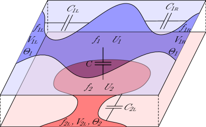
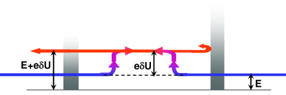
Figure 1: (Color online) Schematic of the double cavity and operation scheme: Electrons enter the cavity, gain an energy $e\delta U$ and then leave the cavity again, experiencing different transmissions of the contacts.

In this paper, we investigate the rectification of thermal fluctuations into a directed electric current in a mesoscopic heat engine. The latter consists of two capacitively coupled chaotic cavities arranged in a three-terminal geometry as shown Fig. 1. The upper cavity is the rectifier and is connected via two contacts with energy-dependent transmissions to electron reservoirs. The lower cavity provides the external source of thermal noise. It is connected via only a single contact to another electron reservoir. The energy dependence of the contact transmissions is a generic feature of mesoscopic conductors and leads to an intrinsic nonlinearity in the upper cavity. Jordan and Büttiker (2008) The three-terminal setup allows for separated heat and charge currents in contrast to two-terminal setups where these currents are necessarily aligned.

The mechanism giving rise to the current is shown schematically in Fig. 1. Electrons enter the cold upper cavity at an energy $E$. They absorb the energy $e\delta U$ from the fluctuating potential generated by the hot lower cavity in the upper cavity and afterwards leave the cold cavity again. As the transmissions through the upper cavity’s contacts are energy-dependent, the ratio between transport processes involving the left and right lead is different at energies $E$ and $E+e\delta U$, thus giving rise to a net electrical current through the cavity. The rectification is controlled by Coulomb coupling which is dominant at low temperatures, whereas at higher temperatures phonon effects become important. Entin-Wohlman et al. (2010)

Thermoelectric properties of both open mesoscopic cavities  Godijn et al. (1999); Llaguno et al. (2003) and in the Coulomb blockade limit Molenkamp et al. (1994); Staring et al. (1993); Dzurak et al. (1997) have been of interest. The quantization of energy levels in small dots leads to exceptional thermo-electrical properties. Edwards et al. (1995) Both in two- and three-terminal structures the limit in which the ratio of electric to heat current is given by the ratio of the charge to an energy quantum can be reached. Humphrey et al. (2002); Sánchez and Büttiker (2011) Still, while the efficiency of such nanoengines can in principle be optimal leading to an infinite figure of merit $ZT$Mahan and Sofo (1996), the current they deliver is small, typically of the order of $1\,\mathrm{pA}$. It is therefore of interest to explore how power output and efficiency scale as dots are opened and turned into cavities with contacts that permit currents that are much larger than the tunneling current of a Coulomb-blockaded quantum dot.

The physics of Coulomb coupled conductors is of interest in nanophysics for on-chip charge detectors, Jordan and Korotkov (2006) quantum Hall edge states, le Sueur et al. (2010) and the Coulomb drag in which one system that carries a current induces a current in a nearby unbiased conductor. Laroche et al. (2011); Mortensen et al. (2001); Levchenko and Kamenev (2008); Sánchez et al. (2010) In the setup of Fig. 1 the current carrying conductor in the Coulomb drag problem is replaced by an unbiased but hot conductor.

Our paper is organized as follows: In Sec. II, we present our model of the double cavity and describe our theoretical approach. Our results are presented in Sec. III and conclusions are drawn in Sec. IV. Calculational details are presented in the Appendices.

II Model and method

We investigate transport through two capacitively coupled open quantum dots with mutual capacitance $C$, cf. Fig 1. Each cavity $i=1,2$ is coupled via quantum point contacts (QPCs) to electronic reservoirs $r=\text{L},\text{R}$. The latter ones are assumed to be in local equilibrium and described by a Fermi distribution $f_{ir}(x)=\{\exp[(x-\mu_{ir})/k_{\text{B}}\Theta_{i}]+1\}^{-1}$ with temperature $\Theta_{i}$ and chemical potential $\mu_{ir}$. Interaction effects are captured by capacitive couplings $C_{ir}$ between the cavities and their respective reservoirs that leads to screening of the potential fluctuations.

We consider the system in the semiclassical limit where the number $N_{ir}$ of open transport channels van Wees et al. (1991); Patel et al. (1991); Rössler et al. (2011) in the QPCs is large under conditions at which dephasing destroys phase information but preserves energy. We can, thus, characterize the chaotic cavities by a distribution function $f_{i}(E)$ that depends on energy only, and focus on a semi-classical description of the physics without coherence. Blanter and Sukhorukov (2000) For later convenience, we write the distribution function as

$$f_{i}=\frac{\sum_{r}T_{ir}f_{ir}}{\sum_{r}T_{ir}}+\delta f_{i}.$$ (1)

Here, the first term describes the average value of $f_{i}$ and is given by the average of the distributions of the reservoirs weighted with the transmission $T_{ir}$ of the respective QPC. The second term $\delta f_{i}$ describes fluctuations of $f_{i}$ around its average. Additionally, each cavity is characterized by its potential $U_{i}$ which also fluctuates by $\delta U_{i}$.

We assume the transmissions to be energy dependent which we model to first order as $T_{ir}=T_{ir}^{0}-eT^{\prime}_{ir}\delta U_{i}$. The energy dependent transmission leads to a nonlinear current voltage characteristic. Even without external noise such a nonlinearity requires a self-consistent treatment. Büttiker (1993); Christen and Büttiker (1996) In our system, Fig. 1, we need a self-consistent treatment not only of the average Hartree potential but in addition the fluctuating potentials. We remark that while the energy-independent part $T^{0}_{ir}$ scales linearly with the number of open transport channels $N_{ir}$, the energy-dependent part $T^{\prime}_{ir}$ is independent of $N_{ir}$.

The starting point of our theoretical investigation is a kinetic equation for the distribution functions $f_{i}$ (see, e.g., Ref. Nagaev et al., 2004),

$$e\nu_{i\text{F}}\frac{df_{i}}{dt}=e\nu_{i\text{F}}\frac{\partial f_{i}}{\partial U_{i}}\dot{U}_{i}+\frac{e}{h}\sum_{r}T_{ir}(f_{ir}-f_{i})+\delta i_{\Sigma},$$ (2)

where $\nu_{i\text{F}}$ denotes the density of states of cavity $i$. It describes the change of charge in a given energy interval due to changes in the potential $U_{i}$, in- and outgoing electron currents through the QPCs as well as their fluctuations $\delta i_{\Sigma}$ where the index $\Sigma$ indicates summation over all contacts $r$ of cavity $i$.

Expressing the charge inside the cavities via the distribution functions $f_{i}$ as well as via the capacitances and potentials, we obtain a relation between $\delta f_{i}$ and $\delta U_{i}$ which allows us to transform the kinetic equation (2) into a Langevin equation for $\delta U_{i}$. Neglecting terms that are cubic and higher in the potential fluctuations, the latter can be converted into a nonlinear Fokker-Planck equation with a diffusion function that depends on the cavity potential. The nonlinearity of the Langevin equation leads to subtleties in the interpretation of the stochastic integral (known as the Itô and Stratonovich problem) that gives rise to different Fokker-Planck equations. The “kinetic prescription” of Klimontovich Klimontovich (1990) provides a steady-state solution of Eq. (2) that is in global thermal equilibrium, thus avoiding the Brillouin paradox mentioned in the introduction.

We stress that the nonlinearity is the technical origin of rectification in the cavity. A linear system would not exhibit this feature. From the Klimontovich-Fokker-Planck equation we obtain $\langle\delta U_{i}\rangle$ and $\langle\delta U_{i}\delta U_{j}\rangle$, cf. Appendixes A-D for details. The charge currents between upper cavity and contact $r$ are given by

$$I_{1r}=\frac{e}{h}\int dET_{1r}(f_{1r}-f_{1})+\delta I_{r}.$$ (3)

III Results

The critical nonlinearity of the cavity is quantified by the amount of symmetry-breaking in the energy-derivatives of the transmissions of the upper cavity, given by the rectification parameter $\Lambda$:

$$\Lambda=\frac{G^{\prime}_{1\text{L}}G_{1\text{R}}-G^{\prime}_{1\text{R}}G_{1\text{L}}}{G_{1\Sigma}^{2}},$$ (4)

where $G_{ir}=(e^{2}/h)T^{0}_{ir}$ and $G^{\prime}_{ir}=(e^{3}/h)T^{\prime}_{ir}$. We will see below that it is the rectification conversion factor between energy and charge for an unbiased cavity. This parameter appears in many places in terms of interaction corrections. For example, if we consider the uncoupled upper cavity ($C=0$, $i=1$), the single cavity conductance $G_{1}=G_{1L}G_{1R}/G_{1\Sigma}$ (which is the series combination of the left and right leads) has an interaction correction of $\Delta G_{1}=-2C_{1\mu}G_{\Sigma}\Lambda^{2}k_{B}\Theta_{1}/C_{1\Sigma}^{2}$, where $C_{1\Sigma}=\sum_{r}C_{1r}$ is the total capacitance of the upper cavity and $C_{1\mu}^{-1}=(e^{2}\nu_{1\text{F}})^{-1}+C_{1\Sigma}^{-1}$ is its electrochemical capacitance. We note that while $G_{1}$ scales with the channel number $N$, the correction $\Delta G_{1}$ is of order $\propto N^{-1}$ (quantum corrections in a coherent cavity Kupferschmidt and Brouwer (2008) are of order $\propto N^{0}$). The rectification parameter $\Lambda$ also appears in the second-order conductance.

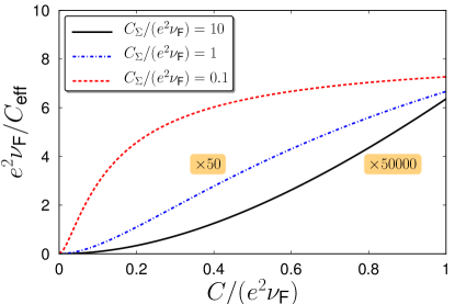
Figure 2: Inverse effective capacitance as a function of the capacitance between the two cavities $C$ for different values of $e^{2}\nu_{\text{F}}/C_{\Sigma}$. Note the different scale for the various curves.

We now turn to the coupled cavities, cf. Fig. 1. Applying different temperatures $\Theta_{1}$ and $\Theta_{2}$ to the reservoirs that couple to cavity 1 and 2, respectively, while keeping the electrical contacts grounded ($V_{ir}=0$), we find to leading order in the nonlinearity a charge current through the cavity given by

$$\langle I_{\text{1L}}\rangle=\frac{\Lambda}{\tau_{RC}}k_{\text{B}}(\Theta_{1}-\Theta_{2}),$$ (5)

where we assumed identical capacitances and densities of states for the two cavities. Now, we give a physical interpretation of each term in Eq. (5), the rectified current. $\tau_{RC}=C_{\text{eff}}/G_{\text{eff}}$ denotes an effective $RC$ time of the double cavity. It is determined by the effective conductance of the double cavity, $G_{\text{eff}}=G_{1\Sigma}G_{2\Sigma}/(G_{1\Sigma}+G_{2\Sigma})$ which is largest if both cavities have equal conductances. Furthermore, it depends on the effective capacitance

$$C_{\text{eff}}=\frac{C_{\Sigma}(2C+C_{\Sigma})(C_{\Sigma}^{2}+2CC_{\Sigma}-CC_{\mu})}{2C^{2}C_{\mu}}$$ (6)

describing how strong the interaction is between the two cavities. It should be minimized (without entering the Coulomb blockade regime) to maximize the rectified current. It grows as $C^{-2}$ and for large couplings approaches the constant value $(2C_{\Sigma}-C_{\mu})C_{\Sigma}/C_{\mu}$, cf. Fig. 2. Next, as stated, the rectified current (5) is proportional to $\Lambda$, which characterizes the asymmetry of the system: The system is asymmetric if either the left-right conductances and/or their energy derivatives differ. Finally, the current (5) is linear in the applied temperature difference, so the rectified current is zero in global thermal equilibrium, as must be the case in order to satisfy the second law of thermodynamics. We note that the sign of the current flips under either exchange of the system lead nonlinearity or under exchange of the cavity temperatures.

As the energy-dependent part of the transmission does not scale with the number of transport channels, the current Eq. (5) also turns out to be independent of the channel number. For realistic values van Wees et al. (1991); Patel et al. (1991); Rössler et al. (2011) of $C_{\text{eff}}=10\,\mathrm{fF}$, $G^{\prime}=(e^{2}/h)\mathrm{(mV)}^{-1}$ and $\Theta_{2}-\Theta_{1}=1\,\mathrm{K}$, we find $I\sim 0.1\,\mathrm{nA}$ which can be readily detected in current experiments and is two orders of magnitude larger than currents through typical Coulomb-blockaded dots.

In order to convert the heat extracted from the hot reservoir into useful work, we have to make the noise-induced current flow against a finite bias voltage $V_{1\text{L}}-V_{1\text{R}}$. The bias induces a counterflow of current given to leading order in the nonlinearity by $G_{1}(V_{1\text{L}}-V_{1\text{R}})$, thus reducing the total current. At the stopping voltage, $V_{\text{stop}}=\Lambda\,k_{\text{B}}(\Theta_{1}-\Theta_{2})/(G_{1}\tau_{RC})$, there is no current flowing through the system. The output power is given by $P=\langle I_{1\text{L}}\rangle(V_{1\text{L}}-V_{1\text{R}})$. It is parabolic as a function of the applied voltage, vanishing at zero bias and the stopping voltage; it has a maximum at half the stopping voltage given by

$$P_{\text{max}}=\frac{\Lambda^{2}}{4G_{1}\tau_{RC}^{2}}(k_{\text{B}}(\Theta_{1}-\Theta_{2}))^{2}.$$ (7)

Energy is transferred between the cavities in the form of dissipated power in the upper cavity, $P=\sum_{r}\langle I_{1r}V_{1r}\rangle$, the heat current given up by the lower hot cavity to the upper cold cavity, $J_{H}=\langle U_{2}I_{2}\rangle$, and the heat current given up by the upper cold cavity to its heat reservoirs, $J_{C}=\sum_{r}\langle(U_{1}-V_{1r})I_{1r}\rangle$. It is straightforward to check that $J_{H}=J_{C}+P$ in our model, so energy is conserved in the system. The efficiency, $\eta$, of the heat-to-charge-current converter is given by the ratio between the output power, $P$ to the inter-cavity heat current, $J_{H}$. To leading order in the energy-dependent transmissions, this heat current is given by

$$J_{H}=\frac{1}{\tau_{RC}}k_{\text{B}}(\Theta_{2}-\Theta_{1}),$$ (8)

because heat will flow from hot to cold even without the nonlinearity. The correction to this result that is linear in the voltage applied across the upper cavity is suppressed by $G^{\prime}_{1r}$ (as it must to satisfy an Onsager relation, see Appendix E). As indicated earlier, the asymmetry parameter $\Lambda$ controls the process of energy-to-charge conversion, $\langle I_{1\text{L}}\rangle/J_{H}$.

The efficiency $\eta=P/J_{H}$ exhibits the same parabolic bias dependence as the output power since the heat current is independent of the applied bias. Hence, for a given temperature difference, the maximal efficiency occurs at maximum power and is given by

$$\eta_{\text{max}}=\frac{\Lambda^{2}}{4G_{1}\tau_{RC}}k_{\text{B}}(\Theta_{2}-\Theta_{1}).$$ (9)

For $G_{1}=5e^{2}/h$ and parameters as above, we estimate $P_{\text{max}}\sim 2\,\mathrm{fW}$ and a maximal efficiency of $\sim 1\%$ of the Carnot efficiency for a device working at liquid-helium temperatures. We note that while the maximal power of the system scales inversely with the number of available transport channels, the maximal efficiency even decreases with the number of channels squared. This is because for a large number of open channels the effect of the energy-dependence of the uppermost channel becomes less important. This effect can be seen in Fig. 3 where the logarithmic derivative of the QPC conductance is plotted, which controls the stopping voltage and other rectification figures of merit in the case where one contact is energy-independent. For a stronger nonlinearity, such as a truly step-like transmission, a nonperturbative analysis is required which could give rise to much higher efficiencies. Sokolov (1998)

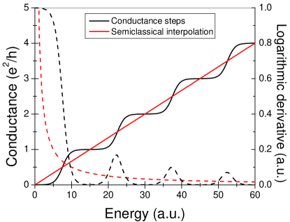
Figure 3: Conductance of a QPC for both fully quantized steps (full black) and semiclassical interpolation (full red). Its logarithmic derivative (black and red dashed) controls the heat-to-charge conversion, stopping voltage, power and efficiency of the energy harvester.

In order to demonstrate that it is the nonlinearity of the rectifying cavity that is the key ingredient to our heat engine, we now briefly consider an alternative setup where a rectifier is coupled to a resistor $R$ at temperature $\Theta_{2}$ with a capacitor $C_{R}$ in parallel instead of a second cavity (see Fig. 4 for a circuit diagram). Repeating the same analysis as above, we find that the heat-induced current, the maximal power as well as the efficiency at maximum power are given by the same expressions as above. The only difference is that the effective conductance and capacitance take on different values, $G_{\text{eff}}\rightarrow G_{1\Sigma}$, $C_{\text{eff}}\rightarrow[C_{R}C_{\Sigma}+C(C_{R}+C_{\Sigma})][C_{\mu}C_{\Sigma}(C+C_{\Sigma})+RG_{\Sigma}(CC_{R}C_{\Sigma}+(C+C_{R})C_{\Sigma}^{2}-CC_{R}C_{\mu})]/(C^{2}C_{\mu}C_{\Sigma})$.

We finally apply our results to the semiclassical regime in the limit $G_{2\Sigma}\gg G_{1\Sigma}$ for simplicity. For large energies the conductance of the QPCs is given by

$$G_{r}(E)=\frac{e^{2}}{h}\frac{(E-E_{r})^{\gamma}}{\Delta_{r}^{\gamma}}\Theta(E-E_{r})$$ (10)

with $E_{r}$ being the energy that marks the transition from tunneling to ballistic transport and $\Delta_{r}$ describing how open the contact is. For equal conductances of the two QPCs at the Fermi energy, $G_{\text{L}}(E_{F})=G_{\text{R}}(E_{F})$, we obtain for the maximal power

$$P_{\text{max}}=\frac{e^{4}}{8h}\frac{\gamma^{2}[k_{\text{B}}(\Theta_{1}-\Theta_{2})]^{2}(1-\mathcal{R})^{2}(E_{F}-E_{\text{L}})^{\gamma-2}}{\Delta_{\text{L}}^{\gamma}C_{\text{eff}}^{2}},$$ (11)

with $\mathcal{R}=\Delta_{\text{L}}/\Delta_{\text{R}}$. We thus see that in order to maximize the power, we need a strong asymmetry in the contacts, $\Delta_{\text{L}}\ll\Delta_{\text{R}}$ while keeping the conductance of each contact the same. For the semiclassical result $\gamma=1/2$, we find that the power drops upon increasing the energy transport window $E_{F}-E_{\text{L}}$. We note, however, that for $\gamma>2$ the contribution from the conductance will outweigh the contribution from the nonlinearity and, thus, lead to a maximal power that increases with the transport window. While the efficiency will drop with the inverse square of the transport window, we remark that a conductance that is exponential in energy will have an efficiency that is independent of the window size.

IV Conclusions

We have examined a mesoscopic energy harvester consisting of a pair of quantum dots and find that as the contacts are opened, the power output can increase but typically with a drop in efficiency for the weak nonlinearity considered here. Our work demonstrates the importance of the asymmetric energy dependence of the contact transmissions. Energy harvesting from environmental fluctuations is an important goal. It might lead to nano-scale devices which can function independently of an external power supply. In densely packed electronic circuits energy harvesting might alleviate the heat removal problem. Our results are useful for future experiments that realize solid state energy harvesters.

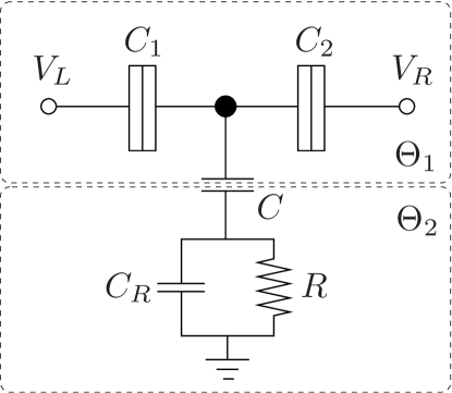
Figure 4: Circuit diagram of a cavity coupled to a hot resistor.

Appendix A Kinetic equation

Our starting point is the set of kinetic equation for the distribution functions $f_{i}$ of the cavities,

$$\frac{df_{i}}{dt}=\frac{\partial f_{i}}{\partial U_{i}}\dot{U}_{i}+\frac{1}{h\nu_{i\text{F}}}\sum_{r}T_{ir}(f_{ir}-f_{i})+\frac{1}{e\nu_{i\text{F}}}\delta i_{\Sigma}.$$ (12)

In the following, we write the distribution function as a constant part that is given by the average of the Fermi functions of the reservoirs weighted with the transmission of the respective QPC and a fluctuating part $\delta f_{i}$:

$$f_{i} =\sum_{r}\frac{T_{ir}f_{ir}}{T_{i\Sigma}}+\delta f_{i}$$

$$=\sum_{r}\frac{G_{ir}}{G_{i\Sigma}}f_{ir}-\Lambda_{i\text{LR}}(f_{i\text{L}}-f_{i\text{R}})\left(\delta U_{i}+\frac{G^{\prime}_{i\Sigma}}{G_{i\Sigma}}(\delta U_{i})^{2}\right)$$

$$\phantom{=}+\delta f_{i}$$ (13)

Here, in the last step, we used $T_{ir}=T^{0}_{ir}-eT^{\prime}_{ir}\delta U_{i}$ and expanded the whole expression up to second order in $\delta U_{i}$. We, furthermore, introduced the asymmetry parameter

$$\Lambda_{i\text{LR}}=\frac{G^{\prime}_{i\text{L}}G_{i\text{R}}-G^{\prime}_{i\text{R}}G_{i\text{L}}}{G_{i\Sigma}^{2}}$$ (14)

and abbreviated $G_{ir}=(e^{2}/h)T^{0}_{ir}$, $G^{\prime}_{ir}=(e^{3}/h)T^{\prime}_{ir}$, where $r=\text{L},\text{R},\Sigma$ refers to the left QPC, the right QPC or the sum over all QPCs adjacent to cavity $i=1,2$.

In order to relate the fluctuating part of the distribution function $\delta f_{i}$ to the fluctuating part of the potential $\delta U_{i}$, we express the charge $Q_{ic}$ inside cavity $i$ once in terms of its distribution function and once in terms of the potentials and capacitances,

$$Q_{ic} =e\nu_{i\text{F}}\int dE\left(\sum_{r}\frac{T_{ir}}{T_{i\Sigma}}f_{ir}+\delta f_{i}\right)-e^{2}\nu_{i\text{F}}U_{i},$$ (15)

$$Q_{ic} =\sum_{i}C_{ir}(U_{i}-V_{ir})+C_{ig}(U_{i}-V_{ig})+C(U_{i}-U_{\bar{i}}),$$ (16)

where $\bar{i}$ denotes the index opposite to $i$. Equating the fluctuating parts of both equations, we find

$$\int dE\delta f_{i}=e\left(\frac{C_{i\Sigma}}{C_{i\mu}}+\frac{\chi_{i}}{e^{3}\nu_{i\text{F}}}\right)\delta U_{i}+\frac{\chi_{i}}{e\nu_{i\text{F}}}\frac{T^{\prime}_{i\Sigma}}{T^{0}_{i\Sigma}}(\delta U_{i})^{2}\\ +e\frac{C}{e^{2}\nu_{i\text{F}}}(\delta U_{i}-\delta U_{\bar{i}}).$$ (17)

Here, we introduced $\chi_{i}=\Lambda_{i\text{LR}}(V_{i\text{L}}-V_{i\text{R}})$, the total capacitance of cavity $i$, $C_{i\Sigma}=\sum_{r}C_{ir}+C_{ig}$, as well as its electrochemical capacitance $C_{i\mu}=e^{2}\nu_{i\text{F}}C_{i\Sigma}/(e^{2}\nu_{i\text{F}}+C_{i\Sigma})$.

Using Eq. (17) to eliminate $\delta f_{i}$ from the energy-integrated kinetic equation (12), we obtain a set of coupled, nonlinear Langevin equations that determine $\delta U_{i}$,

$$\begin{split}(C_{i\Sigma}+C)\dot{\delta U_{i}}-C\dot{\delta U}_{\bar{i}}=&-G_{i\Sigma}\left(\frac{C_{i\Sigma}}{C_{i\mu}}+\frac{\chi_{i}}{e^{3}\nu_{i\text{F}}}\right)\delta U_{i}+G^{\prime}_{i\Sigma}\frac{C_{i\Sigma}}{C_{i\mu}}(\delta U_{i})^{2}+\delta I_{i\Sigma}\\ &-G_{i\Sigma}\frac{C}{e^{2}\nu_{\text{iF}}}(\delta U_{i}-\delta U_{\bar{i}})+G^{\prime}_{i\Sigma}\frac{C}{e^{2}\nu_{\text{iF}}}\left[(\delta U_{i})^{2}-\delta U_{i}\delta U_{\bar{i}}\right]\end{split}$$ (18)

Appendix B Diffusion coefficients

The diffusion in Eq. (18) is characterized by the diffusion coefficients defined as Blanter and Büttiker (2000)

$$\langle\delta I_{ir}(t)\delta I_{ir}(0)\rangle=\frac{2e^{2}}{h}\int dET_{ir}\left[f_{ir}(1-f_{ir})+f_{i}(1-f_{i})+(1-T_{ir})(f_{ir}-f_{i})^{2}\right]\delta(t)=D_{ir}\delta(t).$$ (19)

Importantly, the diffusion coefficients $D_{ir}$ depend themselves on $\delta U_{i}$ through the energy-dependence of the transmissions $T_{ir}$. This leads to a certain ambiguity when converting the Langevin equation into a Fokker-Planck equation, see below. Evaluating the above integral and expanding the diffusion coefficient to linear order in the applied voltage, we obtain

$$D_{ir}=4k_{\text{B}}\Theta_{i}(G_{ir}-G^{\prime}_{ir}\delta U_{i}).$$ (20)

Appendix C Fokker-Planck equation

Given a nonlinear Langevin equation of the form

$$\dot{x_{i}}=f_{i}(\mathbf{x})+g_{ij}(\mathbf{x})\eta_{j}(t)$$ (21)

where $\mathbf{x}=(x_{1},x_{2},\cdots)$ and $\eta_{j}(t)$ is a noise source satisfying $\langle\eta_{j}(t)\rangle=0$ and $\langle\eta_{i}(t)\eta_{j}(t^{\prime})\rangle=\delta_{ij}\delta(t-t^{\prime})$, one can show Lau and Lubensky (2007) that it is equivalent to a Fokker-Planck equation of the form

$$\frac{\partial P}{\partial t}=\frac{\partial}{\partial x_{i}}\left[-\left(f_{i}+\alpha\frac{\partial g_{il}}{\partial x_{k}}g_{kl}\right)P+\frac{1}{2}\frac{\partial}{\partial x_{j}}\left(g_{il}g_{jl}P\right)\right]$$ (22)

where Einstein’s sum convention is implied. The parameter $\alpha$ takes the values $0$ in the Itô prescription, $1/2$ in the Stratonovich prescription and $\alpha=1$ in the Klimontovich prescription. Klimontovich (1990) In our analysis, it turns out that only the Klimontovich prescription gives vanishing currents in global thermal equilibrium. In our problem, we have $g_{ij}=\delta_{ij}g_{i}$ such that the Fokker-Planck equation simplifies to

$$\frac{\partial P}{\partial t}=\frac{\partial}{\partial x_{i}}\left[-\left(f_{i}+\alpha\frac{\partial g_{i}}{\partial x_{i}}g_{i}\right)P+\frac{1}{2}\frac{\partial}{\partial x_{i}}\left(g_{i}^{2}P\right)\right]$$ (23)

Multiplying the Fokker-Planck equation with $x_{k}$ and $x_{k}x_{l}$, respectively, and integrating over all variables $x_{i}$, we obtain the following equations for the expectation values

$$\frac{d}{dt}\langle x_{k}\rangle =\left\langle f_{k}\right\rangle+\alpha\left\langle\frac{\partial g_{k}}{\partial x_{k}}g_{k}\right\rangle,$$ (24)

$$\frac{d}{dt}\langle x_{k}x_{l}\rangle =\left\langle x_{l}f_{k}+x_{k}f_{l}\right\rangle+\alpha\left\langle x_{l}\frac{\partial g_{k}}{\partial x_{k}}g_{k}+x_{k}\frac{\partial g_{l}}{\partial x_{l}}g_{l}\right\rangle$$

$$\phantom{=}+\delta_{kl}\left\langle g_{k}^{2}\right\rangle.$$ (25)

To make a closer connection to the discussion above, we introduce $g_{i}=\sqrt{2\tilde{D}_{i}}$ with the diffusion constants $\tilde{D}_{i}$ and obtain

$$\frac{d}{dt}\langle x_{k}\rangle =\left\langle f_{k}\right\rangle+\alpha\left\langle\frac{\partial\tilde{D}_{k}}{\partial x_{k}}\right\rangle,$$ (26)

$$\frac{d}{dt}\langle x_{k}x_{l}\rangle =\left\langle x_{l}f_{k}+x_{k}f_{l}\right\rangle+\alpha\left\langle x_{l}\frac{\partial\tilde{D}_{k}}{\partial x_{k}}+x_{k}\frac{\partial\tilde{D}_{l}}{\partial x_{l}}\right\rangle$$

$$\phantom{=}+2\delta_{kl}\left\langle\tilde{D}_{k}\right\rangle.$$ (27)

By comparing the equation for $\langle x_{k}\rangle$ with the original Langevin equation, we furthermore obtain for the expectation value of the random currents

$$\left\langle\delta I_{ir}\right\rangle=\left\langle\sqrt{2\tilde{D}_{ir}}\eta_{ir}(t)\right\rangle=\alpha\left\langle\frac{\partial\tilde{D}_{ir}}{\partial x_{i}}\right\rangle.$$ (28)

For the calculation of heat current, we also need correlators of the form $\langle x_{i}g_{ij}(\mathbf{x})\eta_{j}(t)\rangle$. In order to obtain them, we multiply the Langevin equation (21) by $x_{i}$,

$$\frac{1}{2}\frac{d}{dt}x_{i}^{2}=x_{i}f_{i}(\mathbf{x})+x_{i}g_{ij}(\mathbf{x})\eta_{j}(t).$$ (29)

Taking expectation values and equating with Eq. (C), we find

$$\langle x_{i}\delta I_{ir}\rangle=\langle x_{i}\sqrt{2\tilde{D}_{ir}}\eta_{ir}(t)\rangle=\frac{1}{2}\langle\tilde{D}_{ir}\rangle+\alpha\left\langle x_{i}\frac{\partial\tilde{D}_{ir}}{\partial x_{i}}\right\rangle.$$ (30)

Appendix D Charge and heat currents

The charge current between lead $r$ and dot $i$ is given by

$$I_{ir}=\frac{e}{h}\int dE(T^{0}_{ir}-eT^{\prime}_{ir}\delta U_{i})(f_{ir}-f)+\delta I_{ir}$$ (31)

which can be rewritten as

$$I_{ir}=\frac{G_{ir}G_{i\bar{r}}}{G_{i\Sigma}}(V_{ir}-V_{i\bar{r}})-\frac{G^{\prime}_{ir}G_{i\bar{r}}}{G_{i\Sigma}}(V_{ir}-V_{i\bar{r}})\delta U_{i}-\left\{(G_{ir}-G^{\prime}_{ir}\delta U_{i})\left[\left(\frac{C_{i\Sigma}}{C_{i\mu}}+\frac{C}{e^{2}\nu_{i\text{F}}}\right)\delta U_{i}-\frac{C}{e^{2}\nu_{i\text{F}}}\delta U_{\bar{i}}\right]\right\}+\delta I_{ir}.$$ (32)

The expectation value of the fluctuating current part is obtained from Eq. (28).

The heat current between lead $r$ and cavity $i$ is given by $J_{ir}=(U_{i}-V_{ir})I_{ir}$. Without an applied bias voltage, we have $J_{ir}=\delta U_{i}I_{ir}$ and, hence,

$$\langle J_{ir}\rangle=-G_{ir}\left[\left(\frac{C_{i\Sigma}}{C_{i\mu}}+\frac{C}{e^{2}\nu_{i\text{F}}}\right)\langle(\delta U_{i})^{2}\rangle^{(0)}-\frac{C}{e^{2}\nu_{i\text{F}}}\langle\delta U_{i}\delta U_{\bar{i}}\rangle^{(0)}\right]+\langle\delta U_{i}\delta I_{ir}\rangle^{(0)},$$ (33)

where the potential-current correlator can be obtained using Eq. (30). The superscript $(0)$ on the expectation values indicates that they have to be evaluated to zeroth order in the applied bias voltage.

The heat current up to linear order is again given by $J_{ir}=\delta U_{i}I_{ir}$ as both the nonfluctuating part of $U_{i}$ as well as the expectation value of $I_{ir}$ are of first order in the bias voltage. We find

$$\begin{split}\langle J_{ir}\rangle=&\frac{G_{ir}G_{i\bar{r}}}{G_{i\Sigma}}\langle\delta U_{i}\rangle^{(0)}(V_{ir}-V_{i\bar{r}})-\frac{G^{\prime}_{ir}G_{i\bar{r}}}{G_{i\Sigma}}(V_{ir}-V_{i\bar{r}})\langle(\delta U_{i})^{2}\rangle^{(0)}\\ &-G_{ir}\left[\left(\frac{C_{i\Sigma}}{C_{i\mu}}+\frac{C}{e^{2}\nu_{i\text{F}}}\right)\langle(\delta U_{i})^{2}\rangle^{(1)}-\frac{C}{e^{2}\nu_{i\text{F}}}\langle\delta U_{i}\delta U_{\bar{i}}\rangle^{(1)}\right]+\langle\delta U_{i}\delta I_{ir}\rangle^{(1)}.\end{split}$$ (34)

Appendix E Onsager relations

According to Onsager Onsager (1931); Casimir (1945) the linear response coefficients of charge and heat currents as a response to bias voltage and thermal gradients are related to each other. To verify the Onsager relation for our system, we expand the charge current through cavity 1 and the heat current between the two cavities to linear order in the bias $\Delta V$ applied to cavity 1 and the temperature difference $\Delta\Theta$ between the reservoirs of the two cavities,

$$\langle I_{1\text{L}}\rangle =G\Delta V+L\Delta\Theta,$$ (35)

$$\langle J_{2\Sigma}\rangle =M\Delta V+N\Delta\Theta.$$ (36)

In the main text we already found that $L=k_{\text{B}}\Lambda_{1\text{LR}}/\tau_{RC}$. Evaluating similarly the heat current in response to an applied bias voltage, we find $M=-k_{\text{B}}\Theta\Lambda_{1\text{LR}}/\tau_{RC}$ in agreement with the Onsager relation $L=-M/\Theta$.

References

- Brillouin (1950) L. Brillouin, Phys. Rev. 78, 627 (1950).
- Marek (1959) A. Marek, Physica 25, 1358 (1959).
- Van Kampen (1960) N. G. Van Kampen, Physica 26, 585 (1960).
- Sokolov (1998) I. M. Sokolov, Europhys. Lett. 44, 278 (1998).
- Astumian and Hänggi (2002) R. D. Astumian and P. Hänggi, Physics Today 55, 33 (2002).
- Büttiker (1987) M. Büttiker, Z. Phys. B 68, 161 (1987).
- van Kampen (1988) N. G. van Kampen, IBM J. Res. Dev. 32, 107 (1988).
- Blanter and Büttiker (1998) Y. M. Blanter and M. Büttiker, Phys. Rev. Lett. 81, 4040 (1998).
- Olbrich et al. (2009) P. Olbrich, E. L. Ivchenko, R. Ravash, T. Feil, S. D. Danilov, J. Allerdings, D. Weiss, D. Schuh, W. Wegscheider, and S. D. Ganichev, Phys. Rev. Lett. 103, 090603 (2009).
- Olbrich et al. (2011) P. Olbrich, J. Karch, E. L. Ivchenko, J. Kamann, B. März, M. Fehrenbacher, D. Weiss, and S. D. Ganichev, Phys. Rev. B 83, 165320 (2011).
- Jordan and Büttiker (2008) A. N. Jordan and M. Büttiker, Phys. Rev. B 77, 075334 (2008).
- Entin-Wohlman et al. (2010) O. Entin-Wohlman, Y. Imry, and A. Aharony, Phys. Rev. B 82, 115314 (2010).
- Godijn et al. (1999) S. F. Godijn, S. Möller, H. Buhmann, L. W. Molenkamp, and S. A. van Langen, Phys. Rev. Lett. 82, 2927 (1999).
- Llaguno et al. (2003) M. C. Llaguno, J. E. Fischer, A. T. Johnson, and J. Hone, Nano Lett. 4, 45 (2003).
- Molenkamp et al. (1994) L. Molenkamp, A. A. M. Staring, B. W. Alphenaar, H. van Houten, and C. W. J. Beenakker, Semicond. Sci. Technol. 9, 903 (1994).
- Staring et al. (1993) A. A. M. Staring, L. W. Molenkamp, B. W. Alphenaar, H. van Houten, O. J. A. Buyk, M. A. A. Mabesoone, C. W. J. Beenakker, and C. T. Foxon, Europhys. Lett. 22, 57 (1993).
- Dzurak et al. (1997) A. S. Dzurak, C. G. Smith, C. H. W. Barnes, M. Pepper, L. Martín-Moreno, C. T. Liang, D. A. Ritchie, and G. A. C. Jones, Phys. Rev. B 55, R10197 (1997).
- Edwards et al. (1995) H. L. Edwards, Q. Niu, G. A. Georgakis, and A. L. de Lozanne, Phys. Rev. B 52, 5714 (1995).
- Humphrey et al. (2002) T. E. Humphrey, R. Newbury, R. P. Taylor, and H. Linke, Phys. Rev. Lett. 89, 116801 (2002).
- Sánchez and Büttiker (2011) R. Sánchez and M. Büttiker, Phys. Rev. B 83, 085428 (2011).
- Mahan and Sofo (1996) G. D. Mahan and J. O. Sofo, Proc. Natl. Acad. Sci. U.S.A. 93, 7436 (1996).
- Jordan and Korotkov (2006) A. N. Jordan and A. N. Korotkov, Phys. Rev. B 74, 085307 (2006).
- le Sueur et al. (2010) H. le Sueur, C. Altimiras, U. Gennser, A. Cavanna, D. Mailly, and F. Pierre, Phys. Rev. Lett. 105, 056803 (2010).
- Laroche et al. (2011) D. Laroche, G. Gervais, M. P. Lilly, and J. L. Reno, Nat. Nano. 6, 793 (2011).
- Mortensen et al. (2001) N. A. Mortensen, K. Flensberg, and A. Jauho, Phys. Rev. Lett. 86, 1841 (2001).
- Levchenko and Kamenev (2008) A. Levchenko and A. Kamenev, Phys. Rev. Lett. 101, 216806 (2008).
- Sánchez et al. (2010) R. Sánchez, R. López, D. Sánchez, and M. Büttiker, Phys. Rev. Lett. 104, 076801 (2010).
- van Wees et al. (1991) B. J. van Wees, L. P. Kouwenhoven, E. M. M. Willems, C. J. P. M. Harmans, J. E. Mooij, H. van Houten, C. W. J. Beenakker, J. G. Williamson, and C. T. Foxon, Phys. Rev. B 43, 12431 (1991).
- Patel et al. (1991) N. K. Patel, J. T. Nicholls, L. Martn-Moreno, M. Pepper, J. E. F. Frost, D. A. Ritchie, and G. A. C. Jones, Phys. Rev. B 44, 10973 (1991).
- Rössler et al. (2011) C. Rössler, S. Baer, E. de Wiljes, P. Ardelt, T. Ihn, K. Ensslin, C. Reichl, and W. Wegscheider, New J. Phys. 13, 113006 (2011).
- Blanter and Sukhorukov (2000) Y. M. Blanter and E. V. Sukhorukov, Phys. Rev. Lett. 84, 1280 (2000).
- Büttiker (1993) M. Büttiker, J. Phys.: Condens. Matter 5, 9361 (1993).
- Christen and Büttiker (1996) T. Christen and M. Büttiker, Europhys. Lett. 35, 523 (1996).
- Nagaev et al. (2004) K. E. Nagaev, S. Pilgram, and M. Büttiker, Phys. Rev. Lett. 92, 176804 (2004).
- Klimontovich (1990) Y. L. Klimontovich, Phys. A 163, 515 (1990).
- Kupferschmidt and Brouwer (2008) J. N. Kupferschmidt and P. W. Brouwer, Phys. Rev. B 78, 125313 (2008).
- Blanter and Büttiker (2000) Y. M. Blanter and M. Büttiker, Phys. Rep. 336, 1 (2000).
- Lau and Lubensky (2007) A. W. C. Lau and T. C. Lubensky, Phys. Rev. E 76, 011123 (2007).
- Onsager (1931) L. Onsager, Phys. Rev. 37, 405 (1931).
- Casimir (1945) H. B. G. Casimir, Rev. Mod. Phys. 17, 343 (1945).