Capacitary measures for completely monotone kernels via singular control

Abstract

We give a singular control approach to the problem of minimizing an energy functional for measures with given total mass on a compact real interval, when energy is defined in terms of a completely monotone kernel. This problem occurs both in potential theory and when looking for optimal financial order execution strategies under transient price impact. In our setup, measures or order execution strategies are interpreted as singular controls, and the capacitary measure is the unique optimal control. The minimal energy, or equivalently the capacity of the underlying interval, is characterized by means of a nonstandard infinite-dimensional Riccati differential equation, which is analyzed in some detail. We then show that the capacitary measure has two Dirac components at the endpoints of the interval and a continuous Lebesgue density in between. This density can be obtained as the solution of a certain Volterra integral equation of the second kind.

Keywords: Singular control, verification argument, capacity theory, infinite-dimensional Riccati differential equation, optimal order execution, optimal trade execution, transient price impact

AMS Subject Classification: 49J15, 49K15, 31C15, 49N90, 91G80, 34G20

1 Introduction and statement of results

1.1 Background

Let $G:\mathbb{R}_{+}\to\mathbb{R}_{+}$ be a function. The problem of minimizing the energy functional

$$\mathcal{E}(\mu):=\frac{1}{2}\int\int G(|t-s|)\,\mu(ds)\,\mu(dt)$$

over probability measures $\mu$ supported by a given compact set $K\subset\mathbb{R}$ plays an important role in potential theory. A minimizing measure $\mu^{*}$, when it exists, is called a capacitary measure, and the value $\text{Cap}\,(K):=1/\mathcal{E}(\mu^{*})$ is called the capacity of the set $K$; see, e.g., choquet, fuglede, and landkof. See also AikawaEssen or Helms for more recent books on potential theory.

In this paper, we develop a control approach to determining the capacitary distribution $\mu^{*}$ when $K$ is a compact interval and $G$ is a completely monotone function. In this approach, measures $\mu$ on $K$ will be regarded as singular controls and $\mathcal{E}(\mu)$ is the objective function. Our goal is to obtain qualitative structure theorems for the optimal control $\mu^{*}$ and characterize $\mu^{*}$ by means of certain differential and integral equations.

The intuition for this control approach, and in fact our original motivation, come from the problem of optimal order execution in mathematical finance. In this problem, one considers an economic agent who wishes to liquidate a certain asset position of $x$ shares within the time interval $[0,T]$. This asset position can either be a long position ($x>0$) or a short position $(x<0$). The order execution strategy chosen by the investor is described by the asset position $X_{t}$ held at time $t\in[0,T]$. In particular, one must have $X_{0}=x$. Requiring the condition $X_{T+}=0$ assures that the initial position has been unwound by time $T$. The left-continuous path $X=(X_{t})_{t\in[0,T]}$ will be nonincreasing for a pure sell strategy and nondecreasing for a pure buy strategy. A general strategy can consist of both buy and sell trades and hence can be described as the sum of a nonincreasing and a nondecreasing strategy. That is, $X$ is a path of finite variation.

The problem the economic agent is facing is that his or her trades impact the price of the underlying asset. To model price impact, one starts by informally defining $q\,dX_{t}$ as the immediate price impact generated by the (possibly infinitesimal) trade $dX_{t}$ executed at time $t$. Next, it is an empirically well-established fact that price impact is transient and decays over time; see, e.g., MoroEtAl. This decay of price impact can be described informally by requiring that $G(t-s)\,dX_{s}$ is the remaining impact at time $t$ of the impact generated by the trade $dX_{s}$. Here, $G:\mathbb{R}_{+}\to\mathbb{R}_{+}$ is a nonincreasing function with $G(0)=q$, the decay kernel. Thus, $\int_{s<t}G(t-s)\,dX_{s}$ is the price impact of the strategy $X$, cumulated until time $t$. This price impact creates liquidation costs for the economic agent, and one can derive that, under the common martingale assumption for unaffected asset prices, these costs are given by

$$\mathcal{C}(X):=\frac{1}{2}\int_{[0,T]}\int_{[0,T]}G(|t-s|)\,dX_{s}\,dX_{t}$$ (1)

plus a stochastic error term with expectation independent of the specific strategy $X$; see GSS. Indeed, let us assume that asset prices are given by $S^{X}_{t}=S^{0}_{t}+\int_{0}^{t}G(t-s)\,dX_{s}$ where $S^{0}$ is a continuous martingale and $\int_{0}^{t}G(t-s)\,dX_{s}$ models the price impact of the trading strategy at time $t$. Then, we assume that the order $dX_{t}$ is made at the average price $\frac{1}{2}(S^{X}_{t-}+S^{X}_{t})$ and costs $\frac{1}{2}(S^{X}_{t-}+S^{X}_{t})\,dX_{t}$, which corresponds to a block shape limit order book, see AFS2. Accumulating these costs over $[0,T]$, integrating by parts twice, and taking expectations yields

$$\mathbb{E}\left[\int_{[0,T]}\frac{1}{2}(S^{X}_{t-}+S^{X}_{t})\,dX_{t}\right]=-S_{0}^{0}X_{0}+\mathbb{E}[\,\mathcal{C}(X)\,],$$

where we have used the fact that $\mathbb{E}\left[\int_{[0,T]}S^{0}_{t}dX_{t}\right]=-S^{0}_{0}X_{0}$, due to the martingale assumption on $S^{0}$. Further details can be found in GSS.

Thus, minimizing the expected costs amounts to minimizing the functional $\mathcal{C}(X)$ over all left-continuous strategies $X$ that are of bounded variation and satisfy $X_{0}=x$ and $X_{T+}=0$. This problem was formulated and solved in the special case of exponential decay, $G(t)=e^{-\rho t}$, by ow. The general case was analyzed by ASS in discrete time and by GSS in the continuous-time setup we have used above. We refer to AFS2, AS, GSS2, PredoiuShaikhetShreve, SchiedSlynko, and GatheralSchiedSurvey for further discussions and additional references in the context of mathematical finance.

Clearly, the cost functional $\mathcal{C}(X)$ coincides with the energy functional $\mathcal{E}(\nu^{X})$ of the measure $\nu^{X}(dt):=dX_{t}$. So finding an optimal order execution strategy is basically equivalent to determining a capacitary measure for $[0,T]$. There is one important difference, however: capacitary measures are determined as minimizers of $\mathcal{E}(\mu)$ with respect to all nonnegative measures $\mu$ on $[0,T]$ with total mass $1$, while $\nu^{X}$ may be a signed measure with given total mass $\nu^{X}([0,T])=-x$. This difference can become significant if $G(|\cdot|)$ is only required to be positive definite in the sense of Bochner (which is essentially equivalent to $\mathcal{C}(X)\geq 0$ for all $X$), because then minimizers of the unconstrained problem need not exist. It was first shown by ASS, and later extended to continuous time by GSS, that a unique optimal order execution strategy $X^{*}$ exists and that $X^{*}$ is a monotone function of $t$ when $G$ is convex and nonincreasing. This result has the important consequence that the constrained problem of finding a capacitary measure is equivalent to the unconstrained problem of determining an optimal order execution strategy.

In this paper, we aim at describing the structure of capacitary measures/optimal order execution strategies. To this end, it is instructive to first look at two specific examples in which the optimizer is known in explicit form. ow find that for exponential decay, $G(t)=e^{-\rho t}$, the capacitary measure $\mu^{*}$ has two singular components at $t=0$ and $t=T$ and a constant Lebesgue density on $(0,T)$:

$$\mu^{*}(dt)=\frac{1}{2+\rho T}\,\delta_{0}(dt)+\frac{\rho}{2+\rho T}\,dt+\frac{1}{2+\rho T}\,\delta_{T}(dt).$$ (2)

Numerical experiments show that it is a common pattern that capacitary measures for nonincreasing convex kernels have two singular components at $t=0$ and $T=0$ and a Lebesgue density on $(0,T)$. However, the capacitary measure for $G(t)=\max\{0,1-\rho t\}$ is the purely discrete measure

$$\mu^{*}=\frac{1}{2+N}\sum_{i=0}^{N}\Big{(}1-\frac{i}{N+1}\Big{)}\big{(}\delta_{\frac{i}{\rho}}+\delta_{T-\frac{i}{\rho}}\big{)},$$

where $N:=\lfloor\rho T\rfloor$ [GSS, Proposition 2.14].

So it is an interesting question for which nonincreasing, convex kernels $G$ the capacitary measure $\mu^{*}$ has singular components only at $t=0$ and $t=T$ and is (absolutely) continuous on $(0,T)$. It turns out that a sufficient condition is the complete monotonicity of $G$, i.e., $G$ belongs to $C^{\infty}((0,\infty))$ and $(-1)^{n}G^{(n)}$ is nonnegative in $(0,\infty)$ for $n\in\mathbb{N}$. More precisely, we have the following result, which is in fact an immediate corollary of the main results in this paper.

Corollary 1.

Suppose that $G$ is completely monotone with $G^{\prime\prime}(0+):=\lim_{t\downarrow 0}G^{\prime\prime}(t)<\infty$. Then the capacitary measure $\mu^{*}$ has two Dirac components at $t=0$ and $t=T$ and is has a continuous Lebesgue density on $(0,T)$.

1.2 Statement of main results

Our main results do not only give the preceding qualitative statement on the form of $\mu^{*}$ but they also provide quantitative descriptions of the Dirac components of $\mu^{*}$ and of its Lebesgue density on $(0,T)$. To prepare for the statement of these results, let us first assume that $G(0)=1$, which we can do without loss of generality. Then we recall that by the celebrated Hausdorff–Bernstein–Widder theorem [Widder, Theorem IV.12a], $G$ is completely monotone if and only if it is the Laplace transform of a Borel probability measure $\lambda$ on $\mathbb{R}_{+}$:

$$G(t)=\int e^{-\rho t}\,\lambda(d\rho),\qquad t\geq 0.$$

In particular, every exponential polynomial,

$$G(t)=\sum_{i=0}^{d}\lambda_{i}e^{-\rho_{i}t},$$ (3)

with $\lambda_{i},\,\rho_{i}\geq 0$ and $\sum_{i}\lambda_{i}=1$ is completely monotone. Another example is power-law decay,

$$G(t)=\frac{1}{(1+t)^{\gamma}}\qquad\text{for some $\gamma>0$,}$$

which is a popular choice for the decay of price impact in the econophysics literature; see Gatheral and the references therein. We assume henceforth that $G^{\prime\prime}(0+)<\infty$, which is equivalent to

$$\overline{\rho}:=\int\rho\,\lambda(d\rho)<\infty\qquad\text{and}\qquad\overline{\rho^{2}}:=\int\rho^{2}\,\lambda(d\rho)<\infty.$$ (4)

A crucial role will be played by the following infinite-dimensional Riccati equation for functions $\varphi:[0,\infty)\times\mathbb{R}_{+}^{2}\to\mathbb{R}$,

$$\varphi^{\prime}(t,\rho_{1},\rho_{2})+(\rho_{1}+\rho_{2})\varphi(t,\rho_{1},\rho_{2})=\frac{1}{2\overline{\rho}}\Big{(}\rho_{1}+\int x\varphi(t,\rho_{1},x)\,\lambda(dx)\Big{)}\Big{(}\rho_{2}+\int x\varphi(t,x,\rho_{2})\,\lambda(dx)\Big{)}$$ (5)

where $\varphi^{\prime}$ denotes the time derivative of $\varphi$, and the function $\varphi$ satisfies the initial condition

$$\varphi(0,\rho_{1},\rho_{2})=1\qquad\text{for all $\rho_{1},\rho_{2}\geq 0$.}$$ (6)

Remark 1.

When writing (5) in the form $\varphi^{\prime}=F(\varphi)$ one sees that the functional $F$ is not a continuous map from some reasonable function space into itself, unless $\lambda$ is concentrated on a compact interval. For instance, it involves the typically unbounded linear operator $\varphi\mapsto(\rho_{1}+\rho_{2})\varphi$. Therefore, existence and uniqueness of solutions to (5), (6) does not follow by an immediate application of standard results such as the Cauchy–Lipschitz/Picard–Lindelöf theorem in Banach spaces [HillePhillips, Theorem 3.4.1] or more recent ones such as those in Teixeira and the references therein. In fact, even in the simplest case in which $\lambda$ reduces to a Dirac measure, the existence of global solution hinges on the initial condition; it is easy to see that solutions blow up when $\varphi(0)$ is not chosen in a suitable manner.

We now state a result on the global existence and uniqueness of (5), (6). It states that the solution takes values in the locally convex space $C(\mathbb{R}^{2}_{+})$ endowed with topology of locally uniform convergence. For integers $k\geq 0$, the space $C^{k}([0,\infty);C(\mathbb{R}^{2}_{+}))$ will consist of all continuous functions $\varphi:[0,\infty)\to C(\mathbb{R}^{2}_{+})$ which, when considered as functions $\varphi:[0,\infty)\to C(K)$ for some compact subset $K$ of $\mathbb{R}^{2}_{+}$, belong to $C^{k}([0,\infty);C(K))$.

Theorem 1.

When $G^{\prime\prime}(0+)<\infty$ the initial value problem (5), (6) admits a unique solution $\varphi$ in the class of functions $\widetilde{\varphi}$ in $C^{1}([0,\infty);C(\mathbb{R}^{2}_{+}))$ that satisfy an inequality of the form

$$0\leq\widetilde{\varphi}(t,\rho_{1},\rho_{2})\leq c(1+\rho_{1})(1+\rho_{2}),$$ (7)

where $c$ is a constant that may depend on $\varphi$ and locally uniformly on $t$. Moreover, $\varphi$ has the following properties.

1. $\varphi$ is strictly positive.

2. $\varphi$ is symmetric: $\varphi(t,\rho_{1},\rho_{2})=\varphi(t,\rho_{2},\rho_{1})$ for all $(\rho_{1},\rho_{2})\in\mathbb{R}_{+}^{2}$.

3. $1=\int\varphi(t,\rho,x)\,\lambda(dx)=\int\varphi(t,x,\rho)\,\lambda(dx)$ for all $\rho\geq 0$.

4. $\varphi\in C^{2}([0,\infty);C(\mathbb{R}^{2}_{+}))$.

5. For every $t$, the kernel $\varphi(t,\cdot,\cdot)$ is nonnegative definite on $L^{2}(\lambda)$, i.e.,

   $$\int\int f(x)f(y)\varphi(t,x,y)\,\lambda(dx)\,\lambda(dy)\geq 0\qquad\text{for $f\in L^{2}(\lambda)$.}$$ (8)

6. The functions $\varphi(t,\rho_{1},\rho_{2})$ and $\varphi^{\prime}(t,\rho_{1},\rho_{2})$ satisfy local Lipschitz conditions in $(\rho_{1},\rho_{2})$, locally uniformly in $t$.

In Section 1.3 we will discuss computational aspects of the initial value problem (5), (6). In particular, we will discuss its solution when $G$ is an exponential polynomial of the form (3) and we will provide closed-form solutions in the cases $d=1$ and $d=2$.

We can now explain how to use singular control in approaching the minimization of $\mathcal{E}(\mu)$ or $\mathcal{C}(X)$. To this end, using order execution strategies $X=(X_{t})$ will be more convenient than using the formalism of the associated measures $\mu(dt)=dX_{t}$ because of the natural dynamic interpretation of $X$. Henceforth, a $[0,T]$-admissible strategy will be a left-continuous function $(X_{t})$ of bounded variation such that $X_{T+}=0$. Our goal is to minimize the cost functional $\mathcal{C}(X)$ defined in (1) over all $[0,T]$-admissible strategies with fixed initial value $X_{0}=x$. Clearly, this problem is not yet suitable for the application of control techniques since $\mathcal{C}(X)$ depends on the entire path of $X$. We therefore introduce the auxiliary functions

$$E^{X}_{t}(\rho):=\int_{[0,t)}e^{-\rho(t-s)}\,dX_{s},\qquad\text{for }\rho\geq 0.$$ (9)

These functions will play the role of state variables that are controlled by the strategy $X$.

Lemma 1.

For any $[0,T]$-admissible strategy $X$, the function $E_{t}^{X}(\rho)$ is uniformly bounded in $\rho$ and $t$. Moreover,

$$\mathcal{C}(X)=\int_{[0,T)}\int E_{t}^{X}(\rho)\,\lambda(d\rho)\,dX_{t}+\frac{1}{2}\sum_{t\leq T}(\Delta X_{t})^{2},$$ (10)

where $\Delta X_{t}:=X_{t+}-X_{t}$ denotes the jump of $X$ at $t$.

Proof. Clearly, $|E_{t}^{X}(\rho)|\leq\|X\|_{\text{var}}$, where $\|X\|_{\text{var}}$ denotes the total variation of $X$ over $[0,T]$. To obtain (10), we integrate by parts to get

$$\mathcal{C}(X)=\int_{{[0,T)}}\int_{{[0,t)}}{G}(t-s)\,dX_{s}\,dX_{t}+\frac{{G}(0)}{2}\sum_{t\leq T}(\Delta X_{t})^{2}.$$

Now we write $G(t-s)$ as $\int e^{-\rho(t-s)}\,\lambda(d\rho)$ and apply Fubini’s theorem. ∎.

The form (10) of our cost functional is now suitable for the application of control techniques. To state our main result, we let $\varphi$ be the solution of our infinite-dimensional Riccati equation as provided by Theorem 1 and we define

$$\varphi_{0}(t):=\varphi(t,0,0)\qquad\text{and}\qquad\psi(t,\rho):=\int x\varphi(t,x,\rho)\,\lambda(dx)$$ (11)

Theorem 2.

Let $X^{*}$ be the unique optimal strategy in the class of $[0,T]$-admissible strategies with initial value $X_{0}=x$. Then

$$\mathcal{C}(X^{*})=\frac{x^{2}}{2\varphi_{0}(T)}.$$ (12)

Moreover, $X^{*}$ has jumps at $t=0$ and $t=T$ of size

$$\Delta X_{0}^{*}=\Delta X_{T}^{*}=-\frac{\psi(T,0)}{2\overline{\rho}\varphi_{0}(T)}\,x$$

and is continuously differentiable on $(0,T)$. The derivative $\xi(t)=\frac{d}{dt}X^{*}_{t}$ is the unique continuous solution of the Volterra integral equation

$$\xi(t)=f(t)+\int_{0}^{t}K(t,s)\xi(s)\,ds,$$ (13)

where, for

$$\Theta(t,\rho):=\frac{\rho+\psi(t,\rho)}{\psi(t,0)}\int x^{2}\varphi(t,x,0)\,\lambda(dx)-\int x^{2}\varphi(t,x,\rho)\,\lambda(dx)+\rho^{2},$$ (14)

the function $f$ and the kernel $K(\cdot,\cdot)$ are given by

$$f(t)=\frac{\Delta X_{0}^{*}}{2\overline{\rho}}\int e^{-\rho t}\Theta(T-t,\rho)\,\lambda(d\rho),\qquad K(t,s)=\frac{1}{2\overline{\rho}}\int e^{-\rho(t-s)}\Theta(T-t,\rho)\,\lambda(d\rho).$$ (15)

Let us recall that we know in addition from Theorem 2.20 in GSS that $t\in[0,T]\mapsto X^{*}_{t}$ is monotone. The identity (12) immediately yields the following formula for the capacity of a compact interval.

Corollary 2.

If $G^{\prime\prime}(0+)<\infty$, the capacity of a compact interval $[a,b]$ is given by

$$\text{\rm Cap}\,([a,b])=2\varphi_{0}(b-a).$$

1.3 Computational aspects

In general, the Riccati equation (5), (6) cannot be solved explicitly. A closed-form solution exists, however, when $G$ is an exponential polynomial as in (3), i.e., when $\lambda$ has a discrete support. Let us assume that $\lambda(dx)=\sum_{i=0}^{d}\lambda_{i}\delta_{\rho_{i}}(dx)$, with $\rho_{0}=0<\rho_{1}<\dots<\rho_{d}$, $\lambda_{i}\geq 0$, and $\sum_{i=0}^{d}\lambda_{i}=1$. All the input that is needed in Theorem 2 are the values $\varphi_{ij}(t):=\varphi(t,\rho_{i},\rho_{j})$, for $0\leq i,j\leq d$. By Theorem 1, $\varphi(t)$ is a symmetric matrix that solves the following matrix Riccati equation:

$$\varphi^{\prime}=-\varphi M^{(3)}\varphi-\varphi M^{(4)}+M^{(1)}\varphi+M^{(2)},$$ (16)

with $M^{(3)}_{ij}=-\frac{1}{{2\overline{\rho}}}\lambda_{i}\rho_{i}\lambda_{j}\rho_{j}$, $M^{(4)}_{ij}=-\frac{\lambda_{i}\rho_{i}\rho_{j}}{2\overline{\rho}}+\delta_{ij}\rho_{i}$, $M^{(1)}=-(M^{(4)})^{\top}$ and $M^{(2)}_{ij}=\frac{\rho_{i}\rho_{j}}{2\overline{\rho}}$. According to Levin, the solution of this equation is given by

$$\varphi(t)=(R^{(1)}(t)\mathbf{1}+R^{(2)}(t))(R^{(3)}(t)\mathbf{1}+R^{(4)}(t))^{-1},$$

where $\mathbf{1}_{ij}=1$ and

$$R(t)=\left[\begin{matrix}R^{(1)}(t)&R^{(2)}(t)\\ R^{(3)}(t)&R^{(4)}(t)\end{matrix}\right]=\exp\left(t\left[\begin{matrix}M^{(1)}&M^{(2)}\\ M^{(3)}&M^{(4)}\end{matrix}\right]\right).$$

In the special cases $d=1$ and $d=2$, the solution of the Riccati equation (5), (6) becomes even easier and, to some extend, becomes explicit. We demonstrate this first for $d=1$ and then for $d=2$:

Example 1.

In the case $d=1$, $G$ is of the form $G(t)=\lambda+(1-\lambda)e^{-\rho t}$ for some $\lambda\in[0,1)$ and some $\rho>0$. Clearly, we can set $\lambda:=0$ without changing the optimization problem. Then $\overline{\rho}=\rho_{1}=\rho$, and (5) becomes

$$\varphi^{\prime}_{00}=\frac{\rho}{2}\,\varphi_{01}^{2},\quad\varphi^{\prime}_{01}+\rho\varphi_{01}=\frac{\rho}{2}\,(1+\varphi_{11})\varphi_{01},\quad\varphi^{\prime}_{11}+2\rho\varphi_{11}=\frac{\rho}{2}\,(1+\varphi_{11})^{2}.$$

For the initial condition $\varphi_{kl}(0)=1$, the preceding equation has the unique solution $\varphi_{11}\equiv\varphi_{01}\equiv 1$ and $\varphi_{00}(t)=1+\rho t/2$. The condition (59) thus reduces to $0={X_{t}}+E^{X}_{1}(t)\big{(}1+\rho(T-t)\big{)}$, which easily yields (2) as unique solution.

Example 2.

In the case $d=2$, we can assume that $G$ is of the form $G(t)=\lambda_{1}e^{-\rho_{1}t}+\lambda_{2}e^{-\rho_{2}t}$, where $\lambda_{1}+\lambda_{2}=1$. Consider a solution $\varphi_{ij}$ $(i,j=0,\dots,2)$ of the matrix Riccati equation (16) with $\lambda_{0}=0$. We can simplify (16) by using the relation

$$\lambda_{1}\varphi_{i1}+\lambda_{2}\varphi_{i2}=1,\qquad i=0,\dots,2.$$ (17)

Indeed, the equation for $\varphi_{11}$ then becomes

$$\varphi_{11}^{\prime}+2\rho_{1}\varphi_{11}=\frac{1}{2\overline{\rho}}\big{(}\rho_{1}+\lambda_{1}\rho_{1}\varphi_{11}+\lambda_{2}\rho_{2}\varphi_{12}\big{)}^{2}=\frac{1}{2\overline{\rho}}\big{(}\rho_{1}+\rho_{2}+\lambda_{1}(\rho_{1}-\rho_{2})\varphi_{11}\big{)}^{2}.$$

This is an autonomous ODE that, for the initial condition $\varphi_{11}(0)=1$, is solved by

$$\varphi_{11}(t)=c_{1}+\bigg{[}\Big{(}\frac{1}{1-c_{1}}-\frac{1}{4}\frac{\lambda_{1}^{2}(\rho_{1}-\rho_{2})^{2}}{\sqrt{\rho_{1}\rho_{2}\overline{\rho}\check{\rho}}}\Big{)}\exp\Big{(}\frac{2\sqrt{\rho_{1}\rho_{2}\overline{\rho}\check{\rho}}}{\overline{\rho}}\cdot t\Big{)}+\frac{1}{4}\frac{\lambda_{1}^{2}(\rho_{1}-\rho_{2})^{2}}{\sqrt{\rho_{1}\rho_{2}\overline{\rho}\check{\rho}}}\bigg{]}^{-1},$$ (18)

where

$$\check{\rho}:=\lambda_{1}\rho_{2}+\lambda_{2}\rho_{1}\text{ and }c_{1}=\Big{(}\frac{\sqrt{\rho_{1}\overline{\rho}}-\sqrt{\rho_{2}\check{\rho}}}{\lambda_{1}(\rho_{1}-\rho_{2})}\Big{)}^{2}.$$

We can notice that $\varphi_{11}(+\infty)=c_{1}$ and $\varphi_{11}(-\infty)=\Big{(}\frac{\sqrt{\rho_{1}\overline{\rho}}+\sqrt{\rho_{2}\check{\rho}}}{\lambda_{1}(\rho_{1}-\rho_{2})}\Big{)}^{2}$.

Similarly,

$$\varphi_{22}^{\prime}+2\rho_{2}\varphi_{22}=\frac{1}{2\overline{\rho}}\big{(}\rho_{1}+\rho_{2}+\lambda_{2}(\rho_{2}-\rho_{1})\varphi_{22}\big{)}^{2},$$

which for the initial condition $\varphi_{22}(0)=1$ is solved by

$$\varphi_{22}(t)=c_{2}+\bigg{[}\Big{(}\frac{1}{1-c_{2}}-\frac{1}{4}\frac{\lambda_{2}^{2}(\rho_{1}-\rho_{2})^{2}}{\sqrt{\rho_{1}\rho_{2}\overline{\rho}\check{\rho}}}\Big{)}\exp\Big{(}\frac{2\sqrt{\rho_{1}\rho_{2}\overline{\rho}\check{\rho}}}{\overline{\rho}}\cdot t\Big{)}+\frac{1}{4}\frac{\lambda_{2}^{2}(\rho_{1}-\rho_{2})^{2}}{\sqrt{\rho_{1}\rho_{2}\overline{\rho}\check{\rho}}}\bigg{]}^{-1},$$ (19)

where

$$c_{2}=\Big{(}\frac{\sqrt{\rho_{2}\overline{\rho}}-\sqrt{\rho_{1}\check{\rho}}}{\lambda_{2}(\rho_{1}-\rho_{2})}\Big{)}^{2}.$$

From (17) we can now easily compute $\varphi_{12}$.

Next, using once again (17), we find that $\varphi_{01}$ solves

$$\varphi_{01}^{\prime}+\rho_{1}\varphi_{01}=\frac{1}{2\overline{\rho}}\big{(}\rho_{2}+\lambda_{1}(\rho_{1}-\rho_{2})\varphi_{01}\big{)}\big{(}\rho_{1}+\rho_{2}+\lambda_{1}(\rho_{1}-\rho_{2})\varphi_{11}\big{)}.$$

That is,

$$\varphi_{01}^{\prime}+\left[\frac{\rho_{1}\overline{\rho}+\rho_{2}\check{\rho}}{2\overline{\rho}}-\frac{\lambda_{1}^{2}}{2\overline{\rho}}(\rho_{1}-\rho_{2})^{2}\varphi_{11}\right]\varphi_{01}=\frac{\rho_{2}}{2\overline{\rho}}\left[\rho_{1}+\rho_{2}+\lambda_{1}(\rho_{1}-\rho_{2})\varphi_{11}\right].$$ (20)

We set $B_{1}=\frac{1}{4}\frac{\lambda_{1}^{2}(\rho_{1}-\rho_{2})^{2}}{\sqrt{\rho_{1}\rho_{2}\overline{\rho}\check{\rho}}}$, $A_{1}=\frac{1}{1-c_{1}}-B_{1}$, and $k=\frac{\sqrt{\rho_{1}\rho_{2}\overline{\rho}\check{\rho}}}{\overline{\rho}}$, so that $\varphi_{11}(t)=c_{1}+\frac{1}{A_{1}e^{2kt}+B_{1}}$. Then, we can check that $\frac{1}{A_{1}e^{kt}+B_{1}e^{-kt}}$ is a solution of the fundamental system. By using a variation of parameters, we get that the solution of (20) satisfying $\varphi_{01}(0)=1$ is given by

$$\varphi_{01}(t)=\frac{A_{1}\varphi_{01}(+\infty)e^{kt}+B_{1}\varphi_{01}(-\infty)e^{-kt}+C_{01}}{A_{1}e^{kt}+B_{1}e^{-kt}},$$

with

$$\varphi_{01}(\pm\infty)=\frac{\pm\sqrt{\rho_{1}\rho_{2}\overline{\rho}\check{\rho}}-\rho_{2}\check{\rho}}{\lambda_{1}\check{\rho}(\rho_{1}-\rho_{2})}\text{ and }C_{01}=A_{1}(1-\varphi_{01}(+\infty))+B_{1}(1-\varphi_{01}(-\infty)).$$

Then, $\varphi_{02}$ can be easily deduced from (17).

It remains to compute $\varphi_{00}$, which solves

$$\varphi_{00}^{\prime}=\frac{1}{2\overline{\rho}}\left[\rho_{2}+\lambda_{1}(\rho_{1}-\rho_{2})\varphi_{01}\right]^{2}.$$

We set $\tilde{C}_{01}=\lambda_{1}(\rho_{1}-\rho_{2})C_{01}$ and get after some calculations:

$$\varphi_{00}^{\prime}(t) = \frac{1}{2\overline{\rho}}\left[\frac{A_{1}k\frac{\overline{\rho}}{\check{\rho}}e^{kt}-B_{1}k\frac{\overline{\rho}}{\check{\rho}}e^{-kt}+\tilde{C}_{01}}{A_{1}e^{kt}+B_{1}e^{-kt}}\right]^{2}$$

$$= \frac{\rho_{1}\rho_{2}}{2\check{\rho}}+\frac{\tilde{C}_{01}}{\check{\rho}}\frac{A_{1}ke^{kt}-B_{1}ke^{-kt}}{(A_{1}e^{kt}+B_{1}e^{-kt})^{2}}+\frac{\tilde{C}_{01}^{2}\check{\rho}-4A_{1}B_{1}\rho_{1}\rho_{2}\overline{\rho}}{2\overline{\rho}\check{\rho}}\frac{1}{(A_{1}e^{kt}+B_{1}e^{-kt})^{2}}.$$

Thus, we finally get:

$$\varphi_{00}(t) = 1+\frac{\rho_{1}\rho_{2}}{2\check{\rho}}t-\frac{\tilde{C}_{01}}{\check{\rho}}\left(\frac{1}{A_{1}e^{kt}+B_{1}e^{-kt}}-\frac{1}{A_{1}+B_{1}}\right)$$

$$+\frac{\tilde{C}_{01}^{2}\check{\rho}-4A_{1}B_{1}\rho_{1}\rho_{2}\overline{\rho}}{4B_{1}k\overline{\rho}\check{\rho}}\left(\frac{e^{kt}}{A_{1}e^{kt}+B_{1}e^{-kt}}-\frac{1}{A_{1}+B_{1}}\right).$$

This completes this example.

Given the solution $\varphi$ of the Riccati equation, we can approximate the continuous time strategy by a discrete one as follows ($x_{i}$ will denote the trading size at time $iT/N$).

• We first set $x_{0}=\frac{\psi(T,0)}{2\overline{\rho}\varphi_{0}(T)}$ and $E_{0}(\rho_{\ell})=x_{0}$, $0\leq\ell\leq d$.

• Suppose that $1\leq i<N$ and that $x_{i-1}$ and $E_{i-1}(\rho_{\ell})$ have been computed. Then, we set thanks to (59):

  $$x_{i}=1-\sum_{j=0}^{i-1}x_{j}-\int E_{i-1}(\rho)e^{-\rho T/N}\theta(T-iT/N,\rho)\lambda(d\rho),\ E_{i}(\rho_{\ell})=E_{i-1}(\rho_{\ell})e^{-\rho_{\ell}T/N}+x_{i}.$$

• Set $x_{N}=1-\sum_{j=0}^{i-1}x_{j}$.

Alternatively, we could have approximated the minimization of the cost (1) by the following discrete problem. Let $M_{i,j}=G\left(|i-j|\frac{T}{N}\right)$, $0\leq i,j\leq N$, and consider

$$\text{ minimize $\frac{1}{2}x^{T}Mx$ over $x\in\mathbb{R}^{N+1}$ s.t $\sum_{i=0}^{N}x_{i}=1$}.$$ (22)

The solution of this problem is obviously given by $\frac{1}{\mathbf{1}^{T}M^{-1}\mathbf{1}}M^{-1}\mathbf{1}$, where $\mathbf{1}_{i}=1$ for $0\leq i\leq N$. From a financial point of view, the minimization problem (22) gives the optimal strategy when it is only possible to trade at the times $iT/N$, while the original problem (1) allows to trade continuously. In potential theory, it corresponds to computing the capacitary distribution of the set $\{iT/N\,|\,i=0,\dots,N\}$. It was shown in the proof of Theorem 2.20 in GSS that for $N\uparrow\infty$ these cap2acitary distributions converge in the weak topology of probability measures to the capacitary distribution $dX^{*}$ constructed in Theorem 2. Explicit solutions of (22) for the choices $G(t)=e^{-\rho t}$ and $G(t)=(1-\rho t)^{+}$ were given in AFS1 and ASS (note, however, that $G(t)=(1-\rho t)^{+}$ is not completely monotone).

We have computed and plotted the solutions given by both methods in Figure 2 for $T=1$, $N=50$, and $\lambda(d\rho)=0.1\delta_{0}(d\rho)+0.2\delta_{1}(d\rho)+0.2\delta_{3}(d\rho)+0.2\delta_{5}(d\rho)+0.2\delta_{7}(d\rho)+0.1\delta_{10}(d\rho)$. They are already rather close together for $N=50$, and they merge when $N\rightarrow+\infty$. Let us discuss briefly the time complexity of the two methods. The one given by (22) gets very slow when $N$ gets large since it involves the inversion of a $N\times N$ matrix. Instead, when $\lambda$ has a discrete support, the matrix Riccati equation can be solved quickly and the algorithm above has a $O(N)$ time complexity, which is much faster. However, this is no longer true when $\lambda$ does not have discrete support. In that case, we have to approximate $\lambda$ by a discrete measure, which means that we have to increase $d$. Doing so, will slow down the algorithm based on the Riccati equation. A rigorous treatment of the convergence rate and time complexity of both algorithms is beyond the scope of this paper and is left for future research.

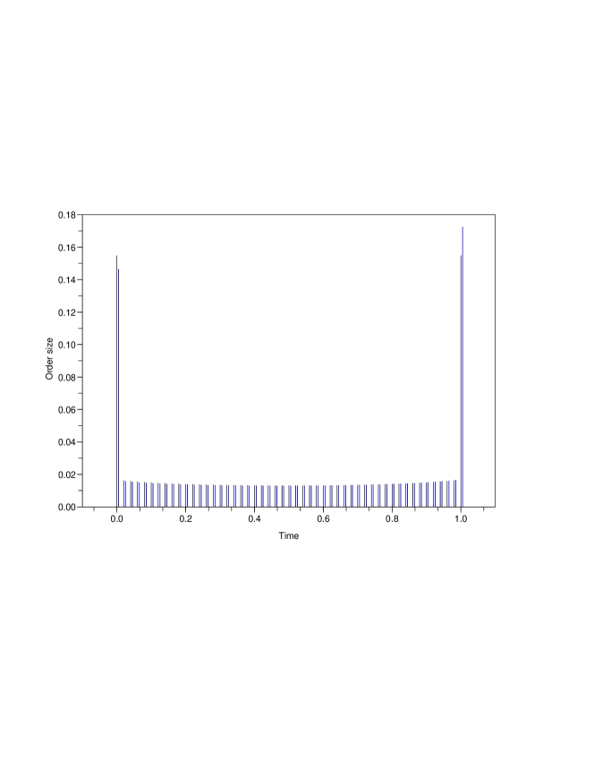
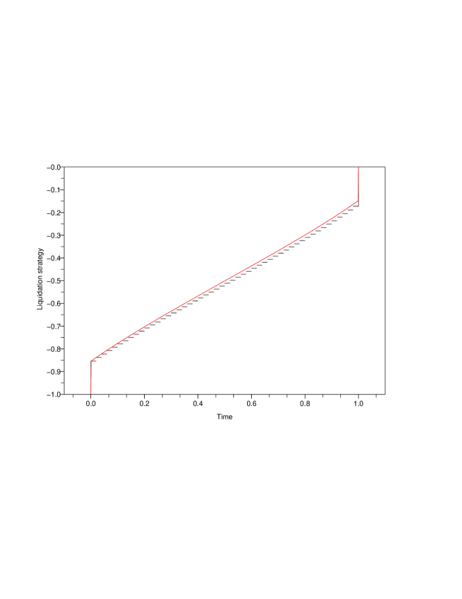
Figure 1: Comparison of the approximated optimal strategies $(x_{i},0\leq i\leq N)$ obtained with (22) and with the method based on the Riccati equation (slightly shifted to the right) .

Figure 2: Comparison of the approximated optimal strategies given by the Riccati method and $N=50$, with the optimal continuous one $X^{*}_{t}$ (computed with $N=1000$) .

2 Proofs

2.1 Proof of Theorem 1

Let us write (5) in the form $\varphi^{\prime}(t)=F_{\lambda}(\varphi(t))$, where

$$F_{\lambda}(f)(\rho_{1},\rho_{2})=-(\rho_{1}+\rho_{2})f(\rho_{1},\rho_{2})+\frac{1}{2\overline{\rho}}\Big{(}\rho_{1}+\int xf(\rho_{1},x)\,\lambda(dx)\Big{)}\Big{(}\rho_{2}+\int xf(x,\rho_{2})\,\lambda(dx)\Big{)}.$$ (23)

Lemma 2.

Suppose that $\lambda$ is supported by the compact interval $[0,\rho_{\max}]$. Then (5), (6) admits a unique solution $\varphi\in C^{1}([0,\infty);C(\mathbb{R}^{2}_{+}))$. Moreover, $\varphi$ has the properties (a), (b), and (c) in the statement of Theorem 1.

Proof. Let $J\subset\mathbb{R}_{+}$ be any compact interval containing $[0,\rho_{\max}]$. Then $F_{\lambda}$ defined in (23) maps $C(J\times J)$ into itself. Moreover, $F_{\lambda}$ is Lipschitz continuous with respect to the sup-norm on every bounded subset of $C(J\times J)$. Hence, the Cauchy–Lipschitz/Picard–Lindelöf theorem in Banach spaces implies the existence of a unique local solution $\varphi_{J}\in C^{1}([0,t_{J});C(J\times J))$ for some maximal time $t_{J}>0$ [HillePhillips, Theorem 3.4.1]. We will show below that $t_{J}=\infty$. Then, if $\widetilde{J}\supset J$ is another compact interval, the restriction of $\varphi_{\widetilde{J}}(t)$ to $J$ must coincide with $\varphi_{J}(t)$ due to the uniqueness of solutions. This consistency then implies the existence and uniqueness of solutions $\varphi\in C^{1}([0,\infty);C(\mathbb{R}^{2}_{+})))$. Moreover, the uniqueness of solutions and the fact that both (5) and (6) are symmetric in $\rho_{1}$ and $\rho_{2}$ implies that $\varphi(t,\rho_{1},\rho_{2})=\varphi(t,\rho_{2},\rho_{1})$ for all $(\rho_{1},\rho_{2})$, which is property (b) in Theorem 1.

We now fix an interval $J\supset[0,\rho_{\max}]$. Before proving that $t_{J}=\infty$, we will show that

$$\int\varphi_{J}(t,\rho,x)\,\lambda(dx)=1\qquad\text{for $\rho\in J$ and $t<t_{J}$.}$$ (24)

This then will establishes property (c) in the statement of Theorem 1 for $t\in[0,t_{J})$. Then we will use (24) to derive some estimates on $\varphi_{J}$ that will yield $\varphi_{J}>0$ and $t_{J}=\infty$.

To prove (24), we let $I(t,\rho):=\int\varphi_{J}(t,\rho,x)\,\lambda(dx)$ and $\psi_{J}(t,\rho):=\int x\varphi_{J}(t,\rho,x)\,\lambda(dx)$. We have

$$I^{\prime}(t,\rho)+\rho I(t,\rho)+\psi_{J}(t,\rho)=\frac{1}{2\overline{\rho}}\big{(}\rho+\psi_{J}(t,\rho)\big{)}\Big{(}\overline{\rho}+\int xI(t,x)\,\lambda(dx)\Big{)}.$$ (25)

This is a (non-homogeneous) affine ODE of the form $I^{\prime}(t)=b(t)+A(t)I(t)$, where the operator

$$(A(t)f)(\rho)=-\rho f(\rho)+\frac{1}{2\overline{\rho}}\big{(}\rho+\psi_{J}(t,\rho)\big{)}\int xf(x)\,\lambda(dx)$$

is a continuous map from $[0,\delta]$ into the space of bounded linear operators on $C(J)$ for each $\delta<t_{J}$. Hence this ODE admits a unique solution in $C^{1}([0,\delta];C(J))$ with initial condition $I(0,\rho)=1$. But (25) is solved by $I(t,\rho)=1$, which which establishes (24).

For the next step, we let

$$t_{0}:=\inf\Big{\{}t\in[0,t_{J})\,\big{|}\,\min_{\rho_{1},\rho_{2}\in J}\varphi_{J}(t,\rho_{1},\rho_{2})<0\Big{\}}.$$

Since $\varphi_{J}$ is a continuous map from $[0,t_{J})$ into $C(J\times J)$ and $\varphi_{J}(0)=1$, we must have $t_{0}>0$. Due to (24) we have on $[0,t_{0})$ that

$$\frac{\rho_{1}\rho_{2}}{2\overline{\rho}}\leq\varphi_{J}^{\prime}(t,\rho_{1},\rho_{2})+(\rho_{1}+\rho_{2})\varphi_{J}(t,\rho_{1},\rho_{2})\leq\frac{(\rho_{1}+\rho_{\max})(\rho_{2}+\rho_{\max})}{2\overline{\rho}}.$$ (26)

When defining

$$\hat{\varphi}_{J}(t,\rho_{1},\rho_{2}):=e^{t(\rho_{1}+\rho_{2})}\varphi_{J}(t,\rho_{1},\rho_{2}),$$ (27)

the preceding inequality can be rewritten as

$$\frac{\rho_{1}\rho_{2}}{2\overline{\rho}}\cdot e^{t(\rho_{1}+\rho_{2})}\leq\hat{\varphi}_{J}^{\prime}(t,\rho_{1},\rho_{2})\leq\frac{(\rho_{1}+\rho_{\max})(\rho_{2}+\rho_{\max})}{2\overline{\rho}}\cdot e^{t(\rho_{1}+\rho_{2})}.$$

Integrating these inequalities yields that for $0\leq t<t_{0}$

$$\varphi_{J}(t,\rho_{1},\rho_{2})\geq e^{-t(\rho_{1}+\rho_{2})}+\frac{\rho_{1}\rho_{2}(1-e^{-t(\rho_{1}+\rho_{2})})}{2\overline{\rho}(\rho_{1}+\rho_{2})}>0$$ (28)

with the convention $\frac{1-e^{-(\rho_{1}+\rho_{2})t}}{\rho_{1}+\rho_{2}}=t$ for $\rho_{1}=\rho_{2}=0$. Hence

$$\varphi_{J}(t,\rho_{1},\rho_{2})\leq e^{-t(\rho_{1}+\rho_{2})}+\frac{(\rho_{1}+\rho_{\max})(\rho_{2}+\rho_{\max})}{{2\overline{\rho}(\rho_{1}+\rho_{2})}}(1-e^{-t(\rho_{1}+\rho_{2})}).$$ (29)

Inequality (28) ensures that $t_{0}\geq t_{J}$. Both inequalities (28) and (29) ensure the solution $\varphi_{J}(t)$ does not explode in finite time, which by standard arguments yields that $t_{J}=+\infty$. This proves the global existence of solutions as well as property (a) in the statement of Theorem 1. ∎

The preceding lemma works only for measures $\lambda$ that are concentrated on a finite interval. To obtain solutions for more general measures $\lambda$, we need to find upper bounds that are independent of $\rho_{\max}$. To this end, we first derive such bounds for the function $\psi(t,\rho)$ defined in (11). By Lemma 2, this function is well-defined whenever $\lambda$ has compact support, and it follows from dominated convergence together with (28) and (29) that $\psi\in C^{1}([0,\infty);C(\mathbb{R}_{+}))$ and that $\psi^{\prime}(t,\rho)=\int x\varphi^{\prime}(t,\rho,x)\,\lambda(dx)$.

Lemma 3.

Under the assumptions of Lemma 2, we have

$$0<\psi(t,\rho)\leq\frac{\overline{\rho^{2}}}{\overline{\rho}}\qquad\text{for all $\rho\geq 0$.}$$ (30)

Proof. The lower bound in (30) is clear from $\varphi>0$. To prove the upper bound, we suppose by way of contradiction that there exist $t$, $\rho$, and $\varepsilon>0$ such that $\psi(t,\rho)\geq\varepsilon+{\overline{\rho^{2}}}/{\overline{\rho}}$. Then there must be a compact interval $J\supset[0,\rho_{\max}]$ such that

$$\tau_{\varepsilon}:=\inf\Big{\{}t\geq 0\,\Big{|}\,\max_{\rho\in J}\psi(t,\rho)\geq\frac{\overline{\rho^{2}}}{\overline{\rho}}+\varepsilon\Big{\}}$$

is finite. Since $\psi(0,\rho)=\overline{\rho}$ and $\overline{\rho}^{2}\leq\overline{\rho^{2}}$, the time $\tau_{\varepsilon}$ must also be strictly positive. Moreover, there exists $\rho_{\varepsilon}\in J$ such that

$$\max_{\rho\in J}\psi(\tau_{\varepsilon},\rho)=\psi(\tau_{\varepsilon},\rho_{\varepsilon})=\frac{\overline{\rho^{2}}}{\overline{\rho}}+\varepsilon.$$

Then $\tau_{\varepsilon}$ is the first time at which the function $t\mapsto\psi(t,\rho_{\varepsilon})$ reaches a new maximum, and so $\psi^{\prime}(\tau_{\varepsilon},\rho_{\varepsilon})\geq 0$.

Integrating (5) with respect to $\rho_{1}\,\lambda(d\rho_{1})$ and evaluating at $\rho_{2}=\rho_{\varepsilon}$ gives

$$\psi^{\prime}(\tau_{\varepsilon},\rho_{\varepsilon})+\rho_{\varepsilon}\psi(\tau_{\varepsilon},\rho_{\varepsilon})+\int\rho^{2}\varphi(\tau_{\varepsilon},\rho,\rho_{\varepsilon})\,\lambda(d\rho)=\frac{1}{2\overline{\rho}}\big{(}\rho_{\varepsilon}+\psi(\tau_{\varepsilon},\rho_{\varepsilon})\big{)}\Big{(}\overline{\rho^{2}}+\int\rho\psi(\tau_{\varepsilon},\rho)\,\lambda(d\rho)\Big{)}.$$ (31)

Since $\int\varphi(\tau_{\varepsilon},\rho,\rho_{\varepsilon})\,\lambda(d\rho)=1$, the Cauchy–Schwarz inequality (or, alternatively, Jensen’s inequality) implies that $\int\rho^{2}\varphi(\tau_{\varepsilon},\rho,\rho_{\varepsilon})\,\lambda(d\rho)\geq\psi(\tau_{\varepsilon},\rho_{\varepsilon})^{2}$. Moreover, the definition of $\rho_{\varepsilon}$ and the fact that $\lambda$ is supported on $J$ yield that $\int\rho\psi(\tau_{\varepsilon},\rho)\,\lambda(d\rho)\leq\overline{\rho}\psi(\tau_{\varepsilon},\rho_{\varepsilon})$. Plugging these two inequalities into (31) leads to

$$\psi^{\prime}(\tau_{\varepsilon},\rho_{\varepsilon}) \leq \frac{1}{2\overline{\rho}}\big{(}\rho_{\varepsilon}+\psi(\tau_{\varepsilon},\rho_{\varepsilon})\big{)}\big{(}\overline{\rho^{2}}+\overline{\rho}\psi(\tau_{\varepsilon},\rho_{\varepsilon})\big{)}-\rho_{\varepsilon}\psi(\tau_{\varepsilon},\rho_{\varepsilon})-\psi(\tau_{\varepsilon},\rho_{\varepsilon})^{2}$$

$$= \frac{\rho_{\varepsilon}\overline{\rho^{2}}}{2\overline{\rho}}+\Big{(}\frac{\overline{\rho^{2}}}{2\overline{\rho}}-\frac{\rho_{\varepsilon}}{2}\Big{)}\psi(\tau_{\varepsilon},\rho_{\varepsilon})-\frac{1}{2}\psi(\tau_{\varepsilon},\rho_{\varepsilon})^{2}=:p(\psi(\tau_{\varepsilon},\rho_{\varepsilon})),$$

where $p(\cdot)$ is a polynomial function of degree two. It has the two roots $-\rho_{\varepsilon}\leq 0$ and ${\overline{\rho^{2}}}/{\overline{\rho}}>0$. Therefore $p(x)<0$ for $x>{\overline{\rho^{2}}}/{\overline{\rho}}$ and in turn $0>p(\psi(\tau_{\varepsilon},\rho_{\varepsilon}))=\psi^{\prime}(\tau_{\varepsilon},\rho_{\varepsilon})$, which contradicts the fact that $\psi^{\prime}(\tau_{\varepsilon},\rho_{\varepsilon})\geq 0$. ∎

Lemma 4.

Under the assumptions of Lemma 2, we have

$$\begin{split}e^{-t(\rho_{1}+\rho_{2})}+&\frac{\rho_{1}\rho_{2}(1-e^{-t(\rho_{1}+\rho_{2})})}{2\overline{\rho}(\rho_{1}+\rho_{2})}\leq\varphi(t,\rho_{1},\rho_{2})\\ &\leq\exp(-(\rho_{1}+\rho_{2})t)+\frac{(\rho_{1}+\frac{\overline{\rho^{2}}}{\overline{\rho}})(\rho_{2}+\frac{\overline{\rho^{2}}}{\overline{\rho}})}{{2\overline{\rho}(\rho_{1}+\rho_{2})}}\big{(}1-\exp(-(\rho_{1}+\rho_{2})t)\big{)},\end{split}$$ (32)

$$-(\rho_{1}+\rho_{2})-\frac{(\rho_{1}+\frac{\overline{\rho^{2}}}{\overline{\rho}})(\rho_{2}+\frac{\overline{\rho^{2}}}{\overline{\rho}})}{{2\overline{\rho}}}\leq\varphi^{\prime}(t,\rho_{1},\rho_{2})\leq\frac{(\rho_{1}+\frac{\overline{\rho^{2}}}{\overline{\rho}})(\rho_{2}+\frac{\overline{\rho^{2}}}{\overline{\rho}})}{{2\overline{\rho}}}.$$ (33)

Proof. The ODE (5) can be rewritten as

$$\varphi^{\prime}(t,\rho_{1},\rho_{2})+(\rho_{1}+\rho_{2})\varphi(t,\rho_{1},\rho_{2})=\frac{1}{2\overline{\rho}}\big{(}\rho_{1}+\psi(t,\rho_{1})\big{)}\big{(}\rho_{2}+\psi(t,\rho_{2})\big{)}.$$ (34)

Defining $\hat{\varphi}$ as in (27) and using the upper bound in (30) thus yields that

$$\frac{\rho_{1}\rho_{2}}{2\overline{\rho}}\cdot e^{t(\rho_{1}+\rho_{2})}\leq\hat{\varphi}^{\prime}(t,\rho_{1},\rho_{2})\leq\frac{(\rho_{1}+\frac{\overline{\rho^{2}}}{\overline{\rho}})(\rho_{2}+\frac{\overline{\rho^{2}}}{\overline{\rho}})}{{2\overline{\rho}}}\cdot e^{t(\rho_{1}+\rho_{2})}.$$ (35)

Arguing as in the final step of the proof Lemma 2 now yields (32). By plugging (32) back into (34) and using once again (30), we obtain (33).∎

Lemma 5.

For all $R$, $T>0$ there exist constants $L_{1}$, $L_{2}\geq 0$ depending only on $R$, $T$, $\overline{\rho}$, and $\overline{\rho^{2}}$ such that for all $t\in[0,T]$ and $\rho_{1},\widetilde{\rho}_{1}\,\rho_{2}\in[0,R]$,

$$|\varphi(t,\rho_{1},\rho_{2})-\varphi(t,\widetilde{\rho}_{1},\rho_{2})|\leq L_{1}|\rho_{1}-\widetilde{\rho}_{1}|\quad\text{}$$ (36)

and

$$|\varphi^{\prime}(t,\rho_{1},\rho_{2})-\varphi^{\prime}(t,\widetilde{\rho}_{1},\rho_{2})|\leq L_{2}|\rho_{1}-\widetilde{\rho}_{1}|.$$ (37)

Proof. We consider $\rho_{1},\widetilde{\rho}_{1},\rho_{2}\geq 0$ and define

$$\Delta\rho_{1}:=\widetilde{\rho}_{1}-\rho_{1},\quad\Delta\varphi(t)=\varphi(t,\widetilde{\rho}_{1},\rho_{2})-\varphi(t,\rho_{1},\rho_{2})\quad\text{and}\quad\Delta\psi(t)=\psi(t,\widetilde{\rho}_{1})-\psi(t,\rho_{1}).$$

By subtracting the equation (34) satisfied by $\varphi(t,\rho_{1},\rho_{2})$ from the corresponding one satisfied by $\varphi(t,\widetilde{\rho}_{1},\rho_{2})$, we get

$$\Delta\varphi^{\prime}(t)+\varphi(t,\widetilde{\rho}_{1},\rho_{2})\Delta\rho_{1}+(\rho_{2}+\rho_{1})\Delta\varphi(t)=\frac{1}{2\overline{\rho}}\Big{(}\rho_{2}+\psi(t,\rho_{2})\Big{)}\Big{(}\Delta\rho_{1}+\Delta\psi(t)\Big{)}.$$ (38)

This equation is a linear non-homogeneous ODE for $\Delta\varphi(t)$ and, since $\Delta\varphi(0)=0$, solved by

$$\Delta\varphi(t)=$$

$$\int_{0}^{t}\left[\Big{(}\frac{1}{2\overline{\rho}}(\rho_{2}+\psi(s,\rho_{2}))-\varphi(s,\widetilde{\rho}_{1},\rho_{2})\Big{)}\Delta\rho_{1}+\frac{1}{2\overline{\rho}}\Big{(}\rho_{2}+\psi(s,\rho_{2})\Big{)}\Delta\psi(s)\right]e^{-(\rho_{1}+\rho_{2})(t-s)}\,ds,$$

Since $|\psi(s,\rho_{2})|\leq{\overline{\rho^{2}}}/{\overline{\rho}}$, we get with (32) and $\sup_{\alpha\geq 0}\frac{1-e^{-\alpha t}}{\alpha}=t$ that

$$|\Delta\varphi(t)|\leq\frac{1}{2\overline{\rho}}\Big{(}\rho_{2}+\frac{\overline{\rho^{2}}}{\overline{\rho}}\Big{)}\int_{0}^{t}\big{(}|\Delta\rho_{1}|+|\Delta\psi(s)|\big{)}\,ds+\bigg{(}1+\frac{(\widetilde{\rho}_{1}+\frac{\overline{\rho^{2}}}{\overline{\rho}})(\rho_{2}+\frac{\overline{\rho^{2}}}{\overline{\rho}})}{{2\overline{\rho}}}T\bigg{)}\int_{0}^{t}|\Delta\rho_{1}|\,ds.$$ (39)

Now, we have that

$$|\Delta\psi(t)| = \Big{|}\int(\varphi(t,\widetilde{\rho}_{1},x)-\varphi(t,\rho_{1},x))x\,\lambda(dx)\Big{|}\leq\int|\varphi(t,\widetilde{\rho}_{1},x)-\varphi(t,\rho_{1},x)|x\,\lambda(dx)$$

$$\leq \frac{\overline{\rho^{2}}}{\overline{\rho}}\int_{0}^{t}\big{(}|\Delta\rho_{1}|+|\Delta\psi(s)|\big{)}\,ds+\bigg{(}\overline{\rho}+\Big{(}\widetilde{\rho}_{1}+\frac{\overline{\rho^{2}}}{\overline{\rho}}\Big{)}\frac{\overline{\rho^{2}}}{\overline{\rho}}T\bigg{)}\int_{0}^{t}|\Delta\rho_{1}|\,ds.$$

For the last inequality, we have used Fubini’s theorem and (39). Now, Gronwall’s Lemma gives:

$$|\Delta\psi(t)|\leq|\Delta\rho_{1}|t\bigg{(}\frac{\overline{\rho^{2}}}{\overline{\rho}}+\overline{\rho}+\Big{(}\widetilde{\rho}_{1}+\frac{\overline{\rho^{2}}}{\overline{\rho}}\Big{)}\frac{\overline{\rho^{2}}}{\overline{\rho}}T\bigg{)}\exp\Big{(}\frac{\overline{\rho^{2}}}{\overline{\rho}}t\Big{)}.$$ (40)

Plugging this back into (39), we get the existence of a constant $L_{1}$, which depends only on $R$, $T$, $\overline{\rho}$, and $\overline{\rho^{2}}$, such that

$$|\Delta\varphi(t)|\leq L_{1}|\Delta\rho_{1}|.$$ (41)

Finally, using (40) and (41) in (38) and recalling the locally uniform bounds (32) and (30) on $\varphi$ and $\psi$ gives (37). ∎

Now drop the assumption that $\lambda$ is supported on a compact interval and aim at proving existence and uniqueness of solutions in this general case. To this end, we take a sequence $R_{n}\uparrow\infty$ for which $\lambda([0,R_{1}])>0$ and define

$$f_{n}:=\frac{1}{\lambda([0,R_{n}])}\mathbbmss{1}_{[0,R_{n}]}\qquad\text{and}\qquad d\lambda_{n}=f_{n}\,d\lambda,$$ (42)

so that each $\lambda_{n}$ satisfies the assumptions of Lemma 2. By $\varphi_{n}$ we denote the corresponding solution of  (5), (6) provided by that lemma. For each $n\geq 1$, we have

$$\overline{\rho}_{n}:=\int\rho\,\lambda_{n}(d\rho)\geq\int_{0}^{R_{1}}\rho\,\lambda(d\rho)=:\overline{\rho}_{0}\quad\text{and}\quad\overline{\rho^{2}_{n}}:=\int\rho^{2}\,\lambda_{n}(d\rho)\leq\frac{\overline{\rho^{2}}}{\lambda([0,R_{1}])}=:\overline{\rho^{2}_{0}}.$$ (43)

Hence, Lemma 4 yields that for each $n$,

$$e^{-t(\rho_{1}+\rho_{2})}+\frac{\rho_{1}\rho_{2}(1-e^{-t(\rho_{1}+\rho_{2})})}{2\overline{\rho}_{0}(\rho_{1}+\rho_{2})}\leq\varphi_{n}(t,\rho_{1},\rho_{2})\leq 1+\frac{(\rho_{1}+\frac{\overline{\rho^{2}_{0}}}{\overline{\rho}_{0}})(\rho_{2}+\frac{\overline{\rho^{2}_{0}}}{\overline{\rho}_{0}})}{{2\overline{\rho}_{0}}}\frac{1-e^{-(\rho_{1}+\rho_{2})t}}{\rho_{1}+\rho_{2}}$$ (44)

and

$$-(\rho_{1}+\rho_{2})-\frac{(\rho_{1}+\frac{\overline{\rho^{2}_{0}}}{\overline{\rho}_{0}})(\rho_{2}+\frac{\overline{\rho^{2}_{0}}}{\overline{\rho}_{0}})}{{2\overline{\rho}_{0}}}\leq\varphi^{\prime}_{n}(t,\rho_{1},\rho_{2})\leq\frac{(\rho_{1}+\frac{\overline{\rho^{2}_{0}}}{\overline{\rho}_{0}})(\rho_{2}+\frac{\overline{\rho^{2}_{0}}}{\overline{\rho}_{0}})}{{2\overline{\rho}_{0}}}.$$ (45)

Similarly, Lemma 5 yields that for all $R$, $T>0$ there is a constant $L\geq 0$ such that for all $n$

$$|\varphi_{n}(t,\rho_{1},\rho_{2})-\varphi_{n}(t,\widetilde{\rho}_{1},\rho_{2})|\leq L|\rho_{1}-\widetilde{\rho}_{1}|\quad\text{for all $t\in[0,T]$, $\rho_{1},\widetilde{\rho}_{1},\rho_{2}\in[0,R]$,}$$ (46)

The inequalities (45), (46) and the Arzela–Ascoli theorem imply that the sequence $(\varphi_{n})_{n\in\mathbb{N}}$ is relatively compact in the class of continuous functions on $[0,T]\times[0,R]^{2}$ whenever $T$, $R>0$, and hence admits a convergent subsequence in that class. By passing to a subsequence arising from a diagonalization argument if necessary, we may assume that there exists a continuous function $\varphi:[0,\infty)\times\mathbb{R}_{+}^{2}\to\mathbb{R}_{+}$ such that $\varphi_{n}\to\varphi$ locally uniformly.

The uniform bounds (44) and dominated convergence imply that

$$\psi_{n}(t,\rho) := \int x\varphi_{n}(t,\rho,x)\,\lambda_{n}(dx)=\int x\varphi_{n}(t,\rho,x)f_{n}(x)\,\lambda(dx)$$ (48)

$$\longrightarrow\int x\varphi(t,\rho,x)\,\lambda(dx)=\psi(t,\rho)$$

locally uniformly in $(t,\rho)$. Hence, $F_{\lambda_{n}}(\varphi_{n}(t))(\rho_{1},\rho_{2})\to F_{\lambda}(\varphi(t))(\rho_{1},\rho_{2})$, locally uniformly in $(t,\rho_{1},\rho_{2})$, where $F_{\lambda_{n}}$ is defined through (23). Since $\varphi_{n}^{\prime}=F_{\lambda_{n}}(\varphi_{n})$, we conclude that $\varphi_{n}^{\prime}\to F_{\lambda}(\varphi)$ locally uniformly in $[0,\infty)\times\mathbb{R}^{2}_{+}$. Moreover, we have for each $n$ that

$$\varphi_{n}(t,\rho_{1},\rho_{2})-1=\int_{0}^{t}\varphi^{\prime}_{n}(s,\rho_{1},\rho_{2})\,ds.$$

The left-hand side of this equation converges to $\varphi(t,\rho_{1},\rho_{2})-1$, whereas the right-hand side converges to $\int_{0}^{t}F_{\lambda}(\varphi(s))(\rho_{1},\rho_{2})\,ds$. This proves that $\varphi$ solves (5) and that $\varphi\in C^{1}([0,\infty);C(\mathbb{R}^{2}_{+}))$.

Remark 2.

By sending $R_{1}$ to infinity in (44) we get that the solution $\varphi$ constructed above satisfies the bounds

$$e^{-t(\rho_{1}+\rho_{2})}+\frac{\rho_{1}\rho_{2}(1-e^{-t(\rho_{1}+\rho_{2})})}{2\overline{\rho}(\rho_{1}+\rho_{2})}\leq\varphi(t,\rho_{1},\rho_{2})\leq 1+\frac{(\rho_{1}+\frac{\overline{\rho^{2}}}{\overline{\rho}})(\rho_{2}+\frac{\overline{\rho^{2}}}{\overline{\rho}})}{{2\overline{\rho}}}\frac{1-e^{-(\rho_{1}+\rho_{2})t}}{\rho_{1}+\rho_{2}}.$$ (49)

From (30), (48), and the lower bound in (49) we get moreover that

$$0<\psi(t,\rho)\leq\frac{\overline{\rho^{2}}}{\overline{\rho}}.$$ (50)

Now we turn to prove the uniqueness of solutions in the class of functions $\varphi\in C^{1}([0,\infty);C(\mathbb{R}^{2}_{+}))$ satisfying a bound of the form (7) To this end, let $\varphi_{1}$ and $\varphi_{2}$ be two solutions in that class and set

$$\delta(t,\rho_{1},\rho_{2})=\varphi_{2}(t,\rho_{1},\rho_{2})-\varphi_{1}(t,\rho_{1},\rho_{2}).$$

We will show that $\|\delta(t)\|_{L^{2}(\widetilde{\lambda}\otimes\widetilde{\lambda})}^{2}=0$ for all $t$, whenever $\widetilde{\lambda}$ is a positive finite Borel measure of the form $\widetilde{\lambda}=\lambda+\mu$, where $\mu$ is a positive finite Borel measure with compact support. Taking, for instance, $\mu$ as the Lebesgue measure on $[0,R]$ will then imply that $\delta(t,\rho_{1},\rho_{2})=0$ for $\rho_{1},\rho_{2}\in[0,R]$. So this will give the uniqueness of solutions.

Let us define $\widetilde{F}_{\lambda}$ as

$$\widetilde{F}_{\lambda}(f)(\rho_{1},\rho_{2})=\frac{1}{2\overline{\rho}}\Big{(}\rho_{1}+\int xf(\rho_{1},x)\,\lambda(dx)\Big{)}\Big{(}\rho_{2}+\int xf(x,\rho_{2})\,\lambda(dx)\Big{)}.$$ (51)

Lemma 6.

We have $\widetilde{F}_{\lambda}(\varphi_{i}(t))\in L^{2}(\widetilde{\lambda}\otimes\widetilde{\lambda})$ and

$$\|\widetilde{F}_{\lambda}(\varphi_{1}(t))-\widetilde{F}_{\lambda}(\varphi_{2}(t))\|_{L^{2}(\widetilde{\lambda}\otimes\widetilde{\lambda})}^{2}\leq C(\|\delta(t)\|_{L^{2}(\widetilde{\lambda}\otimes\widetilde{\lambda})}^{2}+\|\delta(t)\|_{L^{2}(\widetilde{\lambda}\otimes\widetilde{\lambda})}^{4}),$$ (52)

where $C$ is a positive constant that depends only on $\overline{\rho}$ and $\overline{\rho^{2}}$.

Proof. For simplicity, we will drop the argument $t$ throughout the proof. We may write

$$\widetilde{F}_{\lambda}(\varphi_{2})-\widetilde{F}_{\lambda}(\varphi_{1})$$

$$= \frac{1}{2\overline{\rho}}\bigg{[}\int x\delta(\rho_{1},x)\,\lambda(dx)\Big{(}\rho_{2}+\int x\varphi_{1}(x,\rho_{2})\,\lambda(dx)\Big{)}$$

$$+\int x\delta(x,\rho_{2})\,\lambda(dx)\Big{(}\rho_{1}+\int x\varphi_{1}(\rho_{1},x)\,\lambda(dx)\Big{)}+\int x\delta(\rho_{1},x)\,\lambda(dx)\int x\delta(x,\rho_{2})\,\lambda(dx)\bigg{]}.$$

Thus,

$$(\widetilde{F}_{\lambda}(\varphi_{2})-\widetilde{F}_{\lambda}(\varphi_{1}))^{2}$$

$$\leq \frac{3}{4\overline{\rho}^{2}}\Bigg{[}\left(\int x\delta(\rho_{1},x)\,\lambda(dx)\Big{(}\rho_{2}+\int x\varphi_{1}(x,\rho_{2})\,\lambda(dx)\Big{)}\right)^{2}$$

$$+\left(\int x\delta(x,\rho_{2})\,\lambda(dx)\Big{(}\rho_{1}+\int x\varphi_{1}(\rho_{1},x)\,\lambda(dx)\Big{)}\right)^{2}+\left(\int x\delta(\rho_{1},x)\,\lambda(dx)\int x\delta(x,\rho_{2})\,\lambda(dx)\right)^{2}\Bigg{]}.$$

Now we integrate this inequality with respect to $\widetilde{\lambda}(d\rho_{1})\,\widetilde{\lambda}(d\rho_{2})$. The two first terms can be analyzed in the same way. First, we observe that $\int(\rho_{2}+\frac{\overline{\rho^{2}}}{\overline{\rho}})^{2}\,\widetilde{\lambda}(d\rho_{2})$ is finite. Then we note that

$$\left(\int x\delta(\rho_{1},x)\,\lambda(dx)\right)^{2}\leq\overline{\rho^{2}}\int\delta(\rho_{1},x)^{2}\,\lambda(dx)\leq\overline{\rho^{2}}\int\delta(\rho_{1},x)^{2}\,\widetilde{\lambda}(dx).$$ (53)

Hence,

$$\int\left(\int x\delta(\rho_{1},x)\,\lambda(dx)\right)^{2}\,\widetilde{\lambda}(d\rho_{1})\leq\overline{\rho^{2}}\|\delta\|_{L^{2}(\widetilde{\lambda}\otimes\widetilde{\lambda})}^{2}.$$

Thus, the two first terms can be bounded by $C_{0}\|\delta\|_{L^{2}(\widetilde{\lambda}\otimes\widetilde{\lambda})}^{2}$, where $C_{0}$ is a constant that only depends on $\overline{\rho}$ and $\overline{\rho^{2}}$. Using once again (53), we get that the third term can be bounded from above by $C_{1}\|\delta\|_{L^{2}(\widetilde{\lambda}\otimes\widetilde{\lambda})}^{4}$, where the constant $C_{1}$ depends only on $\overline{\rho}$ and $\overline{\rho^{2}}$.∎

Now we differentiate $\delta^{2}$ and integrate over $[0,t]$:

$$\delta(t,\rho_{1},\rho_{2})^{2} = -2\int_{0}^{t}(\rho_{1}+\rho_{2})\delta(s,\rho_{1},\rho_{2})^{2}\,ds$$

$$+2\int_{0}^{t}\delta(s,\rho_{1},\rho_{2})\Big{[}\widetilde{F}_{\lambda}(\varphi_{2}(s))(\rho_{1},\rho_{2})-\widetilde{F}_{\lambda}(\varphi_{1}(s))(\rho_{1},\rho_{2})\Big{]}\,ds$$

$$\leq 2\int_{0}^{t}\delta(s,\rho_{1},\rho_{2})\Big{[}\widetilde{F}_{\lambda}(\varphi_{2}(s))(\rho_{1},\rho_{2})-\widetilde{F}_{\lambda}(\varphi_{1}(s))(\rho_{1},\rho_{2})\Big{]}\,ds.$$

We now integrate w.r.t. $\widetilde{\lambda}(d\rho_{1})\,\widetilde{\lambda}(d\rho_{2})$ and get by using the Cauchy–Schwarz inequality,

$$\|\delta(t,\cdot)\|_{L^{2}(\widetilde{\lambda}\otimes\widetilde{\lambda})}^{2}\leq 2\int_{0}^{t}\|\delta(s,\cdot)\|_{L^{2}(\widetilde{\lambda}\otimes\widetilde{\lambda})}\|\widetilde{F}_{\lambda}(\varphi_{2}(s))-\widetilde{F}_{\lambda}(\varphi_{1}(s))\|_{L^{2}(\widetilde{\lambda}\otimes\widetilde{\lambda})}\,ds.$$

By continuity of $t\rightarrow\|\delta(t,\cdot)\|_{L^{2}(\widetilde{\lambda}\otimes\widetilde{\lambda})}$, we know that for each $T>0$ there is a constant $K$ such that $\|\delta(t,\cdot)\|_{L^{2}(\widetilde{\lambda}\otimes\widetilde{\lambda})}\leq K$ when $t\in[0,T]$. Thus, we get from Lemma 6 that

$$\|\delta(t,\cdot)\|_{L^{2}(\widetilde{\lambda}\otimes\widetilde{\lambda})}^{2}\leq\sqrt{C(1+K^{2})}\int_{0}^{t}\|\delta(s,\cdot)\|_{L^{2}(\widetilde{\lambda}\otimes\widetilde{\lambda})}^{2}\,ds,$$

which in turn gives that $\|\delta(t,\cdot)\|_{L^{2}(\widetilde{\lambda}\otimes\widetilde{\lambda})}^{2}=0$ on $[0,T]$ by Gronwall’s Lemma. This concludes the proof of uniqueness.

Now we turn to proving the properties (a) through (f) in Theorem 1. Property (a) (strict positivity) can be proved just as in the case of a compactly supported measure $\lambda$ in Lemma 2. Property (b) (symmetry) is already clear. Property (c) ($\int\varphi(t,\rho,x)\,\lambda(dx)=1$) follows from the corresponding property of the approximating functions $\varphi_{n}$, the uniform bounds (44), and dominated convergence.

Property (d) states that $\varphi\in C^{2}([0,\infty);C(\mathbb{R}^{2}_{+}))$. By dominated convergence and the bound (45), which also holds for $\varphi^{\prime}$ in place of $\varphi_{n}^{\prime}$, we get that $\psi(t,\rho)$ belongs to $C^{1}([0,\infty);C(\mathbb{R}_{+}))$. Thus, our ODE gives $\varphi^{\prime}\in C^{1}([0,\infty);C(\mathbb{R}^{2}_{+}))$, which proves property (d).

We now prove property (e). It is clearly enough to prove it when $f:\mathbb{R}_{+}\to\mathbb{R}$ is a bounded measurable function with compact support. To this end, let $\hat{\varphi}(t,\rho_{1},\rho_{2}):=e^{t(\rho_{1}+\rho_{2})}\varphi(t,\rho_{1},\rho_{2})$. Then $\hat{\varphi}$ belongs to $C^{1}([0,\infty);C(\mathbb{R}^{2}_{+}))$ and

$$\hat{\varphi}^{\prime}(t,\rho_{1},\rho_{2})=\frac{1}{2\overline{\rho}}\cdot e^{t(\rho_{1}+\rho_{2})}(\rho_{1}+\psi(t,\rho_{1}))(\rho_{2}+\psi(t,\rho_{2})).$$

That is, $\hat{\varphi}^{\prime}(t,\rho_{1},\rho_{2})=g(t,\rho_{1})g(t,\rho_{2})$ for a function $g$. Thus,

$$\int\int f(x_{1})f(x_{2})\hat{\varphi}^{\prime}(t,x_{1},x_{2})\,\lambda(dx_{1})\,\lambda(dx_{2})=\Big{(}\int f(x)g(t,x)\,\lambda(dx)\Big{)}^{2}\geq 0.$$

Since $\hat{\varphi}(t)=1+\int_{0}^{t}\hat{\varphi}^{\prime}(s)\,ds$, we find that $\hat{\varphi}(t)$ is nonnegative definite. Finally, with $\hat{f}(x)=e^{-tx}f(x)$,

$$\int\int f(x_{1})f(x_{2})\varphi(t,x_{1},x_{2})\,\lambda(dx_{1})\,\lambda(dx_{2})=\int\int\hat{f}(x_{1})\hat{f}(x_{2})\hat{\varphi}(t,x_{1},x_{2})\,\lambda(dx_{1})\,\lambda(dx_{2})\geq 0.$$

This establishes property (e) in Theorem 1.

Finally, property (f) (the local Lipschitz property for $\varphi$ and $\varphi^{\prime}$) follows just as in Lemma 5. This concludes the proof of Theorem 1. ∎

2.2 Proof of Theorem 2

The strategy in the proof of Theorem 2 is to use a verification argument and based on guessing the optimal costs $V(T,E(\cdot),x)$ for liquidating $x$ shares over $[0,T]$ with additional and arbitrary initial data $E(\cdot)$. The result of our guess is formula (54) below. We explain its heuristic derivation in Appendix A.

Let $\varphi$ be a solution of the infinite-dimensional Riccati equation  (5), (6). This solution gives rise to a family of linear operators $\Phi_{t}:L^{2}(\lambda)\to L^{2}(\lambda)\cap C(\mathbb{R}_{+})$ defined by

$$\Phi_{t}f(\rho)=\int f(x)\varphi(t,x,\rho)\,\lambda(dx),\qquad f\in L^{2}(\lambda).$$

By (7), $t\mapsto\Phi_{t}f$ is a continuous map into both $L^{2}(\lambda)$ and $C(\mathbb{R}_{+})$ for each $f\in L^{2}(\lambda)$. By the inequality (45), which also hold for $\varphi$ in place of $\varphi_{n}$, $t\mapsto\Phi_{t}f$ is a continuously differentiable map into both $L^{2}(\lambda)$ and $C(\mathbb{R}_{+})$ for each $f\in L^{\infty}(\lambda)$.

For $t\geq 0$, $E(\cdot)\in L^{2}(\lambda)$, and $x\in\mathbb{R}$, we define

$${V}(t,E(\cdot),x):=\frac{1}{2}\Big{[}\frac{1}{\varphi_{0}(t)}\big{(}x-(\Phi_{t}E)(0)\big{)}^{2}-\langle E,\Phi_{t}E\rangle\Big{]},$$ (54)

where $\langle\cdot,\cdot\rangle$ denotes the usual inner product in $L^{2}(\lambda)$. For $t\in[0,T]$ and a $[0,T]$-admissible strategy $X$ we define

$$C^{X}_{t}:=\int_{[0,t)}\int E^{X}_{s}\,d\lambda\,dX_{s}+\frac{1}{2}\sum_{s<t}(\Delta X_{s})^{2}+{V}(T-t,E_{t}^{X},X_{t}).$$

By Lemma 1, the first two terms on the right correspond to the cost accumulated by the strategy up to time $t$. Moreover,

$${V}(0,E_{T}^{X},X_{T})=\frac{1}{2}(X_{T})^{2}-\int E^{X}_{T}\,d\lambda\cdot X_{T}=\frac{1}{2}(\Delta X_{T})^{2}+\int E_{T}^{X}\,d\lambda\cdot\Delta X_{T},$$

due to the requirement $X_{T+}=0$. This gives $C_{T}^{X}=\mathcal{C}(X)$. Our goal is thus to show the following verification lemma: $dC^{X}_{t}\geq 0$ with equality if and only if $X=X^{*}$ for a certain strategy $X^{*}$. This will identify $X^{*}$ as the optimal strategy and ${V}(T,E(\cdot),x)$ as the optimal cost for liquidating $x$ shares over $[0,T]$ with additional initial data $E(\cdot)$ at time $t=0$. In the formalism of potential theory, ${V}(T,0,-1)$ will then be the minimal energy of a probability measure on $[0,T]$.

Lemma 7.

For every $[0,T]$-admissible strategy $X$, $C^{X}_{t}$ is absolutely continuous in $t$ and

$$\frac{dC^{X}_{t}}{dt}=\frac{1}{2}\bigg{[}\frac{\psi(T-t,0)}{\varphi_{0}(T-t)}\big{(}X_{t}-(\Phi_{T-t}E^{X}_{t})(0)\big{)}+\int E^{X}_{t}(\rho)\big{(}\rho+\psi(T-t,\rho)\big{)}\,\lambda(d\rho)\bigg{]}^{2}$$ (55)

for a.e. $t\in[0,T]$.

Proof. Recall the following integration by parts formula for left-continuous functions $\alpha_{t},\,\beta_{t}$ of locally bounded variation:

$$\alpha_{t}\beta_{t}-\alpha_{s}\beta_{s}=\int_{[s,t)}\alpha_{r}\,d\beta_{r}+\int_{[s,t)}\beta_{r}\,d\alpha_{r}+\sum_{r\in[s,t)}\Delta\alpha_{r}\Delta\beta_{r}.$$

It follows that $t\mapsto E^{X}_{t}(\rho)$ is of bounded variation and

$$E^{X}_{t}(\rho)-E^{X}_{s}(\rho)=X_{t}-X_{s}-\rho\int_{s}^{t}E^{X}_{r}(\rho)\,dr$$ (56)

as well as

$$\begin{split}\@ADDCLASS{ltx_eqn_lefteqn}$\displaystyle E^{X}_{t}(\rho_{1})E^{X}_{t}(\rho_{2})-E^{X}_{s}(\rho_{1})E^{X}_{s}(\rho_{2})$\mbox{}\hfil\\ &=\int_{[s,t)}\big{(}E^{X}_{r}(\rho_{1})+E^{X}_{r}(\rho_{2})\big{)}\,dX_{r}-\int_{s}^{t}(\rho_{1}+\rho_{2})E^{X}_{r}(\rho_{1})E^{X}_{r}(\rho_{2})\,dr+\sum_{r\in[s,t)}(\Delta X_{r})^{2}.\end{split}$$ (57)

Therefore,

$$\varphi(T-t,\rho_{1},\rho_{2})E^{X}_{t}(\rho_{1})E_{t}^{X}(\rho_{2})-\varphi(T-s,\rho_{1},\rho_{2})E^{X}_{s}(\rho_{1})E_{s}^{X}(\rho_{2})$$

$$=-\int_{s}^{t}\varphi^{\prime}(T-r,\rho_{1},\rho_{2})E^{X}_{r}(\rho_{1})E_{r}^{X}(\rho_{2})\,dr-\int_{s}^{t}\varphi(T-r,\rho_{1},\rho_{2})E^{X}_{r}(\rho_{1})E_{r}^{X}(\rho_{2})(\rho_{1}+\rho_{2})\,dr$$

$$\qquad+\int_{[s,t)}\varphi(T-r,\rho_{1},\rho_{2})\big{(}E^{X}_{r}(\rho_{1})+E_{r}^{X}(\rho_{2})\big{)}\,dX_{r}+\sum_{r\in[s,t)}\varphi(T-r,\rho_{1},\rho_{2})(\Delta X_{r})^{2}.$$

We have already observed in the proof of Lemma 1 that $|E_{r}^{X}(\rho)|$ is uniformly bounded in $r\in[0,T]$ and $\rho\geq 0$ by the total variation of $X$. Hence we may integrate both sides of the preceding identity with respect to $\lambda(d\rho_{1})\,\lambda(d\rho_{2})$ to obtain, with the symmetry of $\varphi$ and the notation $\widehat{E}^{X}_{t}:=\rho E^{X}_{t}(\rho)$, that

$$\langle E^{X}_{t},\Phi_{T-t}E^{X}_{t}\rangle-\langle E^{X}_{s},\Phi_{T-s}E^{X}_{s}\rangle$$

$$=-\int_{s}^{t}\langle E^{X}_{r},\Phi^{\prime}_{T-r}E_{r}^{X}\rangle\,dr-2\int_{s}^{t}\langle\widehat{E}^{X}_{r},\Phi_{T-r}E^{X}_{r}\rangle\,dr+2\int_{[s,t)}\langle 1,E^{X}_{r}\rangle\,dX_{r}+\sum_{r\in[s,t)}(\Delta X_{r})^{2}.$$

By a similar reasoning we obtain

$$\Phi_{T-t}E^{X}_{t}(0)-\Phi_{T-s}E^{X}_{s}(0)=-\int_{s}^{t}\Phi^{\prime}_{T-r}E^{X}_{r}(0)\,dr-\int_{s}^{t}\Phi_{T-r}\widehat{E}^{X}_{r}(0)\,dr+X_{t}-X_{s}$$

and

$$\big{(}X_{t}-\Phi_{T-t}E^{X}_{t}(0)\big{)}^{2}-\big{(}X_{s}-\Phi_{T-s}E^{X}_{s}(0)\big{)}^{2}=2\int_{s}^{t}\big{(}X_{r}-\Phi_{T-r}E^{X}_{r}(0)\big{)}\big{(}\Phi^{\prime}_{T-r}E^{X}_{r}(0)+\Phi_{T-r}\widehat{E}^{X}_{r}(0)\big{)}\,dr.$$

Using these formulas, we can now compute

$${C^{X}_{t}-C^{X}_{s}} = \frac{1}{2}\int_{s}^{t}\frac{\varphi_{0}^{\prime}(T-r)}{\varphi_{0}^{2}(T-r)}\big{(}X_{r}-\Phi_{T-r}E^{X}_{r}(0)\big{)}^{2}\,dr$$

$$\qquad+\int_{s}^{t}\frac{X_{r}-\Phi_{T-r}E^{X}_{r}(0)}{\varphi_{0}(T-r)}\big{(}\Phi^{\prime}_{T-r}E^{X}_{r}(0)+\Phi_{T-r}\widehat{E}^{X}_{r}(0)\big{)}\,dr$$

$$\qquad+\frac{1}{2}\int_{s}^{t}\langle E^{X}_{r},\Phi^{\prime}_{T-r}E_{r}^{X}\rangle\,dr+\int_{s}^{t}\langle\widehat{E}^{X}_{r},\Phi_{T-r}E^{X}_{r}\rangle\,dr$$

Therefore, $C^{X}_{t}$ is absolutely continuous on $[0,T]$ and has the derivative

$$\frac{dC^{X}_{t}}{dt} =\frac{1}{2}\frac{\varphi_{0}^{\prime}(T-t)}{\varphi_{0}^{2}(T-t)}\big{(}X_{t}-\Phi_{T-t}E^{X}_{t}(0)\big{)}^{2}$$

$$\qquad+\frac{X_{t}-\Phi_{T-t}E^{X}_{t}(0)}{\varphi_{0}(T-t)}\big{(}\Phi^{\prime}_{T-t}E^{X}_{t}(0)+\Phi_{T-t}\widehat{E}^{X}_{t}(0)\big{)}+\frac{1}{2}\langle E^{X}_{t},\Phi^{\prime}_{T-t}E_{t}^{X}\rangle+\langle\widehat{E}^{X}_{t},\Phi_{T-t}E^{X}_{t}\rangle$$

for a.e. $t$.

To further analyze the preceding formula, we take an extra point $\Delta$. We let $\overline{\lambda}:=\lambda+\delta_{\Delta}$ and extend $E^{X}_{t}$ and $\varphi$ to functions on $\{\Delta\}\cup[0,\infty)$ by putting

$$\begin{split}E^{X}_{t}(\Delta)&:=\frac{1}{\varphi_{0}(T-t)}\big{(}X_{t}-(\Phi_{T-t}E^{X}_{t})(0)\big{)},\\ t\geq 0,\varphi(t,\Delta,\rho)=\varphi(t,\rho,\Delta)&:=\varphi(t,0,\rho),\\ \varphi(t,\Delta,\Delta)&:=\varphi(t,0,0)=\varphi_{0}(t).\end{split}$$ (58)

We furthermore define the function

$$f(x)=\begin{cases}x&\text{if $x\in[0,\infty)$,}\\ 0&\text{if $x=\Delta$,}\end{cases}$$

and we extend the definition of $\widehat{E}^{X}$ via $\widehat{E}^{X}_{t}(x)=f(x)E^{X}_{t}(x)$ for $x\in\{\Delta\}\cup[0,\infty)$. Finally, we set for $g\in L^{2}(\overline{\lambda})$, $\overline{\Phi}_{t}g(x)=\int\varphi(t,x,y)g(y)\overline{\lambda}(dy)$ and one easily checks that $\overline{\Phi}:L^{2}(\overline{\lambda})\rightarrow L^{2}(\overline{\lambda})$.

With this notation, we get

$$\frac{dC^{X}_{t}}{dt} = \frac{1}{2}\langle E^{X}_{t},\overline{\Phi}^{\prime}_{T-t}E^{X}_{t}\rangle_{L^{2}(\overline{\lambda})}+\langle E^{X}_{t},\overline{\Phi}_{T-t}\widehat{E}^{X}_{t}\rangle_{L^{2}(\overline{\lambda})}$$

$$= \frac{1}{2}\Big{[}\langle E^{X}_{t},\overline{\Phi}^{\prime}_{T-t}E^{X}_{t}\rangle_{L^{2}(\overline{\lambda})}+\langle E^{X}_{t},\overline{\Phi}_{T-t}\widehat{E}^{X}_{t}\rangle_{L^{2}(\overline{\lambda})}+\langle\overline{\Phi}_{T-t}E^{X}_{t},\widehat{E}^{X}_{t}\rangle_{L^{2}(\overline{\lambda})}\Big{]}$$

$$= \frac{1}{2}\int\int E^{X}_{t}(x)E^{X}_{t}(y)\Big{(}\varphi^{\prime}({T-t},x,y)+(f(x)+f(y))\varphi({T-t},x,y)\Big{)}\,\overline{\lambda}(dx)\,\overline{\lambda}(dy)$$

$$= \frac{1}{2}\int\int E^{X}_{t}(x)E^{X}_{t}(y)\big{(}f(x)+\psi({T-t},x)\big{)}\big{(}f(y)+\psi({T-t},y)\big{)}\,\overline{\lambda}(dx)\,\overline{\lambda}(dy)$$

$$= \frac{1}{2}\bigg{(}\int E^{X}_{t}(x)\big{(}f(x)+\psi({T-t},x)\big{)}\,\overline{\lambda}(dx)\bigg{)}^{2},$$

where we have used the Riccati equation (5) and the notation (11) in the fourth step. This proves the assertion.∎

It follows from the above that a $[0,T]$-admissible strategy $X^{*}$ with $X^{*}_{0}=x$ satisfies

$$\mathcal{C}(X^{*})=V(T,0,x)\leq\mathcal{C}(X)$$

for all other $[0,T]$-admissible strategies $X$ with $X_{0}=x$ if $dC^{X^{*}}_{t}/dt$ vanishes for a.e. $t\in[0,T]$. Using (55), we write this latter condition as

$$0=X^{*}_{t}+\int E^{X^{*}}_{t}(\rho)\theta(T-t,\rho)\,\lambda(d\rho)\qquad\text{for a.e. $t$},$$ (59)

where

$$\theta(\tau,\rho)=\frac{\varphi_{0}(\tau)(\rho+\psi(\tau,\rho))}{\psi(\tau,0)}-\varphi(\tau,\rho,0).$$

Then

$$\int\theta(\tau,\rho)\,\lambda(d\rho)=\frac{\varphi_{0}(\tau)2\overline{\rho}}{\psi(\tau,0)}-1.$$ (60)

Plugging this and (56) into (59) yields that for a.e. $t$

$$X^{*}_{t}=X^{*}_{0}\Big{(}1-\frac{\psi(T-t,0)}{\varphi_{0}(T-t)2\overline{\rho}}\Big{)}+\frac{\psi(T-t,0)}{\varphi_{0}(T-t)2\overline{\rho}}\int_{0}^{t}\int\rho E^{X^{*}}_{s}(\rho)\theta(T-t,\rho)\,\lambda(d\rho)\,ds.$$ (61)

Thus, the left-continuous function $X^{*}_{t}$ coincides with an absolutely continuous function for a.e. $t\in[0,T]$. It follows that these two functions coincide for every $t\in(0,T]$. Thus, $E^{X^{*}}$ is continuous on $(0,T]$ by (56), which in turn implies via (61) that $X^{*}$ is continuously differentiable throughout $(0,T)$.

When taking the limit $t\downarrow 0$ in (61), we get

$$X^{*}_{0+}=x\Big{(}1-\frac{\psi(T,0)}{\varphi_{0}(T)2\overline{\rho}}\Big{)},$$

which gives

$$\Delta X_{0}^{*}=-\frac{\psi(T,0)}{2\overline{\rho}\varphi_{0}(T)}\,x.$$ (62)

That $\Delta X^{*}_{0}=\Delta X_{T}^{*}$ follows from Remark 2.10 in GSS.

Since $\psi(t,\rho)$ is continuously differentiable in $t$, $\theta(t,\rho)$ is also continuously differentiable in $t$. Differentiating (59) with respect to $t\in(0,T)$ yields

$$0 = \frac{d}{dt}X^{*}_{t}+\int\frac{dE^{X^{*}}_{t}(\rho)}{dt}\theta(T-t,\rho)\,\lambda(d\rho)-\int E^{X^{*}}_{t}(\rho)\theta^{\prime}(T-t,\rho)\,\lambda(d\rho)$$

$$= \frac{2\overline{\rho}\varphi_{0}(T-t)}{\psi(T-t,0)}\cdot\frac{d}{dt}X^{*}_{t}-\int E^{X^{*}}_{t}(\rho)\big{(}\theta^{\prime}(T-t,\rho)+\rho\theta(T-t,\rho)\big{)}\,\lambda(d\rho),$$

where we have used (56) and (60) in the second step. This gives

$$\frac{d}{dt}X^{*}_{t}=\frac{\psi(T-t,0)}{2\overline{\rho}\varphi_{0}(T-t)}\int E^{X^{*}}_{t}(x)\big{(}\theta^{\prime}(T-t,x)+x\theta(T-t,x)\big{)}\,\lambda(dx).$$ (63)

We now want to simplify (63). To this end, we use the notation $\overline{\psi}(t):=\int x\psi(t,x)\,\lambda(dx).$ and the formulas

$$\varphi^{\prime}(t,\rho,0) = -\rho\varphi(t,\rho,0)+\frac{1}{2\overline{\rho}}(\rho+\psi(t,\rho))\psi(t,0),\qquad\varphi_{0}^{\prime}(t)=\frac{1}{2\overline{\rho}}\psi(t,0)^{2}$$

$$\psi^{\prime}(t,\rho) = -\int x^{2}\varphi(t,x,\rho)\,\lambda(dx)-\rho\psi(t,\rho)+\frac{1}{2\overline{\rho}}(\rho+\psi(t,\rho))(\overline{\rho^{2}}+\overline{\psi}(t))$$ (64)

$$\psi^{\prime}(t,0) = -\int x^{2}\varphi(t,x,0)\,\lambda(dx)+\frac{1}{2\overline{\rho}}\psi(t,0)(\overline{\rho^{2}}+\overline{\psi}(t)),$$

Then a tedious computation shows that

$$\theta^{\prime}(t,\rho)+\rho\theta(t,\rho)=\frac{\varphi_{0}(t)}{\psi(t,0)}\cdot\Theta(t,\rho),$$

where $\Theta(t,\rho)$ is as in (14). Therefore, (63) becomes

$$\frac{d}{dt}X^{*}_{t}=\frac{1}{2\overline{\rho}}\int E^{X^{*}}_{t}(x)\Theta(T-t,x)\,\lambda(dx).$$ (65)

Now we have $E^{X^{*}}_{t}=\Delta X^{*}_{0}+\int_{0}^{t}e^{-\rho(t-s)}\frac{d}{dt}X^{*}_{t}\,ds$. Plugging this formula back into (65) and using Fubini’s theorem yields that $\xi(t)=\frac{d}{dt}X^{*}_{t}$ solves the Volterra integral equation (13). This is a Volterra integral equation of the second kind with continuous kernel $K(t,s)$ and continuous function $f(t)$. It hence admits a unique continuous solution $x(\cdot)$ [Linz, Theorem 3.1]. Conversely, given such a solution $x(\cdot)$, we can define a $[0,T]$-admissible strategy $X^{*}$ via (62) and $x(t)=\frac{d}{dt}X^{*}_{t}$. Then $X^{*}$ satisfies (61) for $t=0+$ as well as (63) for $t>0$. Integrating (63) and reversing the steps made above in deriving (63) from (61) shows that $X^{*}$ satisfies (61) for $t\in(0,T]$, and so $X^{*}$ is optimal. This concludes the proof of Theorem 2.∎

Appendix A Heuristic derivation of the value function

We want to explain here how it is possible to guess the value function ${V}(t,E(\cdot),x)$ introduced in (54). We start our discussion by deriving a formula for the costs $\mathcal{C}(X)$ of a strategy $(X_{s},s\in[0,T])$ that is arbitrary on $[0,t)$ and optimal on $[t,T]$. We set

$$\widetilde{\mathcal{C}}_{t}(X) := \mathcal{C}(X)-\frac{1}{2}\int_{[0,t)}\int_{[0,t)}G([s-r|)\,dX_{r}\,dX_{s}$$

$$= \frac{1}{2}\int_{[t,T]}\int_{[t,T]}G([s-r|)\,dX_{r}\,dX_{s}+\int_{[0,t)}\int_{[t,T]}G(|s-r|)\,dX_{s}\,dX_{r}.$$

The rightmost integral can be written as

$$\int_{[t,T]}\int_{[0,t)}G(|s-r|)\,dX_{r}\,dX_{s}=\int_{[t,T]}A(s)\,dX_{s},$$

where

$$A(s)=\int E^{X}_{t}(\rho)e^{-\rho(s-t)}\lambda(d\rho),\qquad t\leq s\leq T.$$

The first-order condition of optimality thus reads

$$\int_{[t,T]}G(|s-r|)\,dX_{r}+A(s)=\nu\qquad\text{for $t\leq s\leq T$,}$$ (66)

where $\nu$ is a suitable Lagrange multiplier (compare Theorem 2.11 in GSS).

Lemma 8.

Suppose that $R$ and $\widetilde{R}$ are functions with finite variation such that $R_{T}=\widetilde{R}_{T}$ and

$$\int_{[t,T]}G(|s-r|)\,dR_{s}=\int_{[t,T]}G(|s-r|)\,d\widetilde{R}_{s}\qquad\text{for all $r\in[t,T]$.}$$

Then $R_{s}=\widetilde{R}_{s}$ for all $s\in[t,T]$.

Proof. We have $\int_{[t,T]}G(|s-r|)\,d(R_{s}-\widetilde{R}_{s})=0$ and hence that

$$\int_{[t,T]}\int_{[t,T]}G(|s-r|)\,d(R_{s}-\widetilde{R}_{s})\,d(R_{r}-\widetilde{R}_{r})=0,$$

which implies the assertion in view of the fact that $G$ is strictly positive definite.∎

Now suppose that we have auxiliary functions with finite variation $B_{t}(\rho)$ such that $B_{T}(\rho)=0$ and

$$\int_{[t,T]}G(|s-r|)\,dB_{r}(\rho)=e^{-\rho(s-t)}\qquad\text{ for }t\leq s\leq T.$$

We also define

$$Z_{s}:=\int E_{t}^{X}(\rho)B_{s}(\rho)\lambda(d\rho),$$

so that

$$A(s)=\int_{[t,T]}G(|s-r|)\,dZ_{r},\text{ for }t\leq s\leq T.$$ (67)

Therefore,

$$\int_{[t,T]}G(|s-r|)\,d(X_{r}+Z_{r})=\nu=\nu\int_{[t,T]}G(|s-r|)\,dB_{r}(0)\qquad\text{for $t\leq s\leq T$}.$$

Lemma 8 hence implies that $X_{s}+Z_{s}=\nu B_{s}(0)\quad\text{for $t\leq s\leq T$.}$ Hence, we get

$$\nu=\frac{X_{t}+Z_{t}}{B_{t}(0)},\ X_{s}=\frac{X_{t}+Z_{t}}{B_{t}(0)}\,B_{s}(0)-Z_{s}\qquad\text{for $s\in[t,T]$.}$$

From these identities we get

$$\widetilde{\mathcal{C}}_{t}(X) = \frac{1}{2}\int_{[t,T]}\int_{[t,T]}G([s-r|)\,dX_{r}\,dX_{s}+\int_{[t,T]}A(s)\,dX_{s}$$

$$= \frac{1}{2}\nu^{2}\int_{[t,T]}\int_{[t,T]}G(|s-r|)\,dB_{r}(0)\,dB_{s}(0)-\nu\int_{[t,T]}\int_{[t,T]}G(|s-r|)\,dB_{r}(0)\,dZ_{s}$$

$$+\frac{1}{2}\int_{[t,T]}\int_{[t,T]}G(|s-r|)\,dZ_{r}\,dZ_{s}+\int_{[t,T]}\int_{[t,T]}G(|s-r|)\,dZ_{r}\,dX_{s}$$

$$= \frac{1}{2}\bigg{[}\frac{(X_{t}+Z_{t})^{2}}{-B_{t}(0)}-\int_{[t,T]}\int_{[t,T]}G(|s-r|)\,dZ_{r}\,dZ_{s}\bigg{]},$$

since the first double integral is equal to $-B_{t}(0)$. Now we define

$$\varphi(T-t,\rho_{1},\rho_{2}):=\int_{[t,T]}e^{-\rho_{1}(r-t)}\,dB_{r}(\rho_{2}),\qquad\rho_{1},\rho_{2}\geq 0.$$

Then, we have

$$\varphi(T-t,\rho_{1},\rho_{2}) = \int_{[t,T]}\int_{[t,T]}G(|r-s|)\,dB_{s}(\rho_{1})\,dB_{r}(\rho_{2})=\varphi(T-t,\rho_{2},\rho_{1}),$$

$$\int\varphi(T-t,\rho_{1},\rho_{2})\,\lambda(d\rho_{1}) = \int_{[t,T]}G(r-t)dB_{r}(\rho_{2})=1.$$

Moreover, we observe that $\varphi(T-t,0,\rho)=-B_{t}(\rho)$ since $B_{T}(\rho)=0$. This gives in particular that $Z_{t}=-\int E^{X}_{t}(\rho)\varphi(T-t,0,\rho)\lambda(d\rho)$. Besides, we have

$$\int_{[t,T]}\int_{[t,T]}G(|s-r|)\,dZ_{r}\,dZ_{s} = \int_{[t,T]}A(s)\,dZ_{s}$$

$$= \int E^{X}_{t}(\rho_{1})\int_{[t,T]}e^{-\rho_{1}(s-t)}\,dZ_{s}\,\lambda(d\rho_{1})$$

$$= \int\int E^{X}_{t}(\rho_{1})E^{X}_{t}(\rho_{2})\int_{[t,T]}e^{-\rho_{1}(s-t)}\,dB_{s}(\rho_{2})\,\lambda(d\rho_{1})\,\lambda(d\rho_{2})$$

$$= \int\int E^{X}_{t}(\rho_{1})E^{X}_{t}(\rho_{2})\varphi(T-t,\rho_{1},\rho_{2})\,\lambda(d\rho_{1})\,\lambda(d\rho_{2}).$$

Thus, we obtain altogether that

$$\widetilde{\mathcal{C}}_{t}(X)=\frac{1}{2}\bigg{[}\frac{\Big{(}X_{t}-\int E^{X}_{t}(\rho)\varphi(T-t,0,\rho)\lambda(d\rho)\Big{)}^{2}}{\varphi(T-t,0,0)}-\int\int E^{X}_{t}(\rho_{1})E^{X}_{t}(\rho_{2})\varphi(T-t,\rho_{1},\rho_{2})\,\lambda(d\rho_{1})\,\lambda(d\rho_{2})\bigg{]}.$$

This suggests the definition

$$V(t,E(.),X):=\frac{1}{2}\bigg{[}\frac{\Big{(}X-\int E(\rho)\varphi(T-t,0,\rho)\lambda(d\rho)\Big{)}^{2}}{\varphi(t,0,0)}-\int\int E(\rho_{1})E(\rho_{2})\varphi(t,\rho_{1},\rho_{2})\,\lambda(d\rho_{1})\,\lambda(d\rho_{2})\bigg{]},$$

so that we have

$$\mathcal{C}(X)=\int_{[0,t)}\int E^{X}_{s}(\rho)\,\lambda(d\rho)\,dX_{s}+\frac{1}{2}\sum_{s<t}(\Delta X_{s})^{2}+V(T-t,E_{t}(.),X_{t}).$$ (68)

Thus, we have obtained the formula given by (54), and it remains to explain why $\varphi$ should solve a Riccati equation. To do so, we consider an arbitrary strategy $(X_{s},s\in[0,T])$ and consider the cost (68), which is the cost of the strategy that is equal to $X$ on $[0,t)$ and optimal on $[t,T]$. To make the dependence on $t$ explicit, we denote this cost by $\mathcal{C}_{t}(X)$. To simplify things, we will focus on the particular case (3) of a discrete measure $\lambda(dx)=\sum_{i=0}^{d}\lambda_{i}\delta_{\rho_{i}}(dx)$, with $\rho_{0}=0<\rho_{1}<\dots<\rho_{d}$, $\lambda_{i}\geq 0$, and $\sum_{i=0}^{d}\lambda_{i}=1$. With this choice, $V$ only depends on $E(\rho_{i})$, $0\leq i\leq d$. We introduce the following notations:

$$\varphi_{ij}(t) = \varphi(t,\rho_{i},\rho_{j}),0\leq i,j\leq d,$$

$$V(t,E_{0},\dots,E_{d},X) = \frac{1}{2}\bigg{[}\frac{1}{\varphi_{00}(t)}\Big{(}X-\sum_{i=0}^{d}\lambda_{i}E_{i}\varphi_{0i}(t)\Big{)}^{2}-\sum_{i=0}^{d}\sum_{j=0}^{d}\lambda_{i}\lambda_{j}E_{i}E_{j}\varphi_{ij}(t)\bigg{]},$$

$$\overline{E}^{X}_{t} = \sum_{i=0}^{d}\lambda_{i}E^{X}_{t}(\rho_{i}),$$

$$\mathcal{C}_{t}(X) = \int_{[0,t)}\overline{E}^{X}_{s}\,dX_{s}+\frac{1}{2}\sum_{s<t}(\Delta X_{s})^{2}+V(T-t,E^{X}_{t}(\rho_{0}),\dots,E^{X}_{t}(\rho_{d}),X_{t}).$$

Lemma 9.

We have $\Delta\mathcal{C}_{t}(X)=0$ for all $t\in[0,T]$.

Proof. Note that $\Delta X_{t}=\Delta E^{X}_{t}(\rho)$. Hence it is clear that $\Delta\mathcal{C}_{t}(X)=0$ if $\Delta X_{t}=0$. Now suppose that $\Delta X_{t}\neq 0$. Then

$$\Delta\mathcal{C}_{t}(X)=\sum_{i=0}^{d}\lambda_{i}E^{X}_{t}(\rho_{i})\Delta X_{t}+\frac{1}{2}(\Delta X_{t})^{2}+\Delta\widetilde{\mathcal{C}}_{t}(X).$$ (69)

On the other hand, we have

$$V(t,E_{0}+\delta,\dots,E_{d}+\delta,X+\delta)$$

$$= \frac{1}{2}\bigg{[}\frac{1}{\varphi_{00}(t)}\Big{(}X+\delta-\sum_{i=0}^{d}\lambda_{i}(E_{i}+\delta)\varphi_{0i}(t)\Big{)}^{2}-\sum_{i=0}^{d}\sum_{j=0}^{d}\lambda_{i}\lambda_{j}(E_{i}+\delta)(E_{j}+\delta)\varphi_{ij}(t)\bigg{]}$$

$$= V(t,E_{0},\dots,E_{d},X)-\delta\sum_{j=0}^{d}\sum_{i=0}^{d}\lambda_{i}\lambda_{j}E_{i}\varphi_{ij}(t)-\frac{\delta^{2}}{2}\sum_{j=0}^{d}\sum_{i=0}^{d}\lambda_{i}\lambda_{j}\varphi_{ij}(t)$$

$$= V(t,E_{0},\dots,E_{d},X)-\delta\sum_{i=0}^{d}\lambda_{i}E_{i}-\frac{\delta^{2}}{2}.$$

Here we have used the facts that $\sum_{i}\lambda_{i}=1$ and $\sum_{i}\lambda_{i}\varphi_{ij}=1$. Putting everything together yields the assertion. ∎

We can now focus on infinitesimal variations, and we denote $V_{t}:=\partial V/\partial t$, $V_{i}:=\partial V/\partial E_{i}$ and $V_{X}:=\partial V/\partial X$. We have, when $\Delta X_{t}=0$,

$$d\mathcal{C}_{t}(X) = \overline{E}^{X}_{t}\,dX_{t}-V_{t}\,dt+\sum_{i=0}^{d}V_{i}\,dE^{X}_{t}(\rho_{i})+V_{X}\,dX_{t}$$

$$= \Big{(}\overline{E}^{X}_{t}+\sum_{i=0}^{d}V_{i}+V_{X}\Big{)}\,dX_{t}-\Big{(}V_{t}+\sum_{i=0}^{d}\rho_{i}E^{X}_{t}(\rho_{i})V_{i}\Big{)}\,dt$$

By simple calculations, we get $\overline{E}^{X}_{t}+\sum_{i=0}^{d}V_{i}+V_{X}=0$, and our expression simplifies to

$$d\mathcal{C}_{t}(X)=-\Big{(}V_{t}+\sum_{i=0}^{d}\rho_{i}E^{X}_{t}(\rho_{i})V_{i}\Big{)}\,dt.$$

Let us now calculate $V_{t}$:

$$V_{t}=-\frac{\varphi_{00}^{\prime}}{2\varphi_{00}^{2}}\Big{(}X-\sum_{j=0}^{d}\lambda_{j}E_{j}\varphi_{0j}\Big{)}^{2}-\sum_{i=0}^{d}\lambda_{i}E_{i}\Big{(}X-\sum_{j=0}^{d}\lambda_{j}E_{j}\varphi_{0j}\Big{)}\frac{\varphi^{\prime}_{0i}}{\varphi_{00}}-\frac{1}{2}\sum_{i,j=0}^{d}\lambda_{i}\lambda_{j}E_{i}E_{j}\varphi_{ij}^{\prime}.$$

To simplify computations, we define

$$\lambda_{-1}:=1\qquad\text{ and}\qquad E_{-1}:=\frac{X-\sum_{j=0}^{d}\lambda_{j}E_{j}\varphi_{0j}}{\varphi_{00}}$$ (70)

as well as $\varphi_{-1i}:=\varphi_{0i}$ and $\varphi_{-1-1}=\varphi_{00}$. Then

$$V_{t}=-\frac{1}{2}\sum_{i,j=-1}^{d}\lambda_{i}E_{i}\lambda_{j}E_{j}\varphi_{ij}^{\prime}.$$

With $\rho_{-1}:=\rho_{0}=0$, we get $V_{i}=-\lambda_{i}\Big{(}\lambda_{-1}E_{-1}\varphi_{-1i}+\sum_{j=0}^{d}\lambda_{j}E_{j}\varphi_{ij}\Big{)}=-\lambda_{i}\sum_{j=-1}^{d}\lambda_{j}E_{j}\varphi_{ij}$ and therefore

$$\sum_{i=0}^{d}\rho_{i}E_{i}V_{i}=-\sum_{i,j=-1}^{d}\frac{\rho_{i}+\rho_{j}}{2}\lambda_{i}E_{i}\lambda_{j}E_{j}\varphi_{ij}.$$

Altogether, we obtain

$$d\mathcal{C}_{t}(X)=\frac{1}{2}\Big{(}\sum_{i,j=-1}^{d}\lambda_{i}E^{X}_{t}(\rho_{i})\lambda_{j}E^{X}_{t}(\rho_{j})\big{(}\varphi_{ij}^{\prime}+({\rho_{i}+\rho_{j}})\varphi_{ij}\big{)}\Big{)}\,dt,$$

where $E^{X}_{t}(\rho_{-1})$ is defined according to (70).

Thus, we arrive at the following quadratic form $\frac{1}{2}\sum_{k,l=0}^{d}E_{k}E_{l}\lambda_{k}\lambda_{l}(\varphi^{\prime}_{kl}+(\rho_{k}+\rho_{l})\varphi_{kl})$. Since we should have $d\mathcal{C}_{t}(X)\geq 0$ with $d\mathcal{C}_{t}(X)=0$ for the optimal strategy, this quadratic form should be nonnegative with rank one. Indeed, since the control $X$ is of dimension one, it would not be possible to make $d\mathcal{C}_{t}(X)=0$ if the rank of the quadratic form were higher than two. We are now going to write the conditions that ensures that this quadratic form is nonnegative with rank one. To do so, We introduce the new coordinates $(\Delta_{0},\dots,\Delta_{d})$ such that

$$E_{0}=\Delta_{0},\quad E_{1}=\Delta_{0}+\Delta_{1},\quad\cdots\quad E_{d}=\Delta_{0}+\Delta_{d}.$$

In these coordinates, our quadratic form becomes

$$\frac{1}{2}\Delta_{0}^{2}\lambda_{0}^{2}(\varphi_{00}^{\prime}+2\rho_{0}\varphi_{00})+\sum_{l=1}^{d}\Delta_{0}(\Delta_{0}+\Delta_{l})\lambda_{0}\lambda_{l}(\varphi_{0l}^{\prime}+(\rho_{0}+\rho_{l})\varphi_{0l})$$

$$+\frac{1}{2}\sum_{k=1}^{d}\sum_{l=1}^{d}(\Delta_{0}+\Delta_{k})(\Delta_{0}+\Delta_{l})\lambda_{k}\lambda_{l}(\varphi_{kl}^{\prime}+(\rho_{k}+\rho_{l})\varphi_{kl})$$

After some calculations, we get that the coefficient for $\Delta_{0}^{2}$, $\Delta_{0}\Delta_{l}$, $\Delta_{k}\Delta_{l}$ and $\Delta_{l}^{2}$ (for $1\leq k,l\leq d$) are respectively $\overline{\rho}$, $\lambda_{l}\Big{(}\rho_{l}+\sum_{k=0}^{d}\lambda_{k}\rho_{k}\varphi_{kl}\Big{)}$, $\lambda_{k}\lambda_{l}(\varphi_{kl}^{\prime}+(\rho_{k}+\rho_{l})\varphi_{kl})$ and $\frac{1}{2}\lambda_{l}^{2}(\varphi_{ll}^{\prime}+2\rho_{l}\varphi_{ll})$.

Thus, the matrix ${\bm{Q}}$ for the quadratic form has coefficients

$${\bm{Q}}_{00} = \overline{\rho},$$

$${\bm{Q}}_{0l}={\bm{Q}}_{l0} = \frac{\lambda_{l}}{2}\Big{(}\rho_{l}+\sum_{k=0}^{d}\lambda_{k}\rho_{k}\varphi_{kl}\Big{)},$$

$${\bm{Q}}_{kl}={\bm{Q}}_{lk} = \frac{1}{2}\lambda_{k}\lambda_{l}(\varphi_{kl}^{\prime}+(\rho_{k}+\rho_{l})\varphi_{kl})\qquad\text{if $k,l\geq 2$, $k\neq l$,}$$

$${\bm{Q}}_{ll} = \frac{1}{2}\lambda_{l}^{2}(\varphi_{ll}^{\prime}+2\rho_{l}\varphi_{ll}).$$

Since ${\bm{Q}}$ is of rank one, the determinant of the matrices

$$\left(\begin{array}[]{cc}{\bm{Q}}_{00}&{\bm{Q}}_{0l}\\ {\bm{Q}}_{l0}&{\bm{Q}}_{ll}\end{array}\right),\ \left(\begin{array}[]{cc}{\bm{Q}}_{00}&{\bm{Q}}_{0l}\\ {\bm{Q}}_{k0}&{\bm{Q}}_{kl}\end{array}\right)$$

must vanish for $l=1,\dots,d$ and $k<l$. That gives, respectively,

$$\varphi_{ll}^{\prime}+2\rho_{l}\varphi_{ll} = \frac{1}{2{\overline{\rho}}}\Big{(}\rho_{l}+\sum_{k=0}^{d}\lambda_{k}\rho_{k}\varphi_{kl}\Big{)}^{2},$$

$$\varphi_{kl}^{\prime}+(\rho_{k}+\rho_{l})\varphi_{kl} = \frac{1}{2{\overline{\rho}}}\Big{(}\rho_{l}+\sum_{i=0}^{d}\lambda_{i}\rho_{i}\varphi_{il}\Big{)}\Big{(}\rho_{k}+\sum_{j=0}^{d}\lambda_{j}\rho_{j}\varphi_{kj}\Big{)},$$ (71)

which gives precisely the Riccati equation. Thus, equation (71) holds for $1\leq k,l\leq d$. In fact, the choice of $E_{0}=\Delta_{0}$ is arbitrary. Had we chosen $E_{i}=\Delta_{i}$ for some $i>0$, we had obtained (71) for $k,l\neq i$. Therefore (71) holds in fact for all $k,l=0,\dots,d$.

References

• [1] \harvarditemAikawa \harvardand Essén1996AikawaEssen Aikawa, H. \harvardand Essén, M. \harvardyearleft1996\harvardyearright, Potential theory—selected topics, Vol. 1633 of Lecture Notes in Mathematics, Springer-Verlag, Berlin.
• [2] \harvarditem[Alfonsi et al.]Alfonsi, Fruth \harvardand Schied2008AFS1 Alfonsi, A., Fruth, A. \harvardand Schied, A. \harvardyearleft2008\harvardyearright, ‘Constrained portfolio liquidation in a limit order book model’, Banach Center Publications 83, 9–25.
• [3] \harvarditem[Alfonsi et al.]Alfonsi, Fruth \harvardand Schied2010AFS2 Alfonsi, A., Fruth, A. \harvardand Schied, A. \harvardyearleft2010\harvardyearright, ‘Optimal execution strategies in limit order books with general shape functions’, Quant. Finance 10, 143–157.
• [4] \harvarditemAlfonsi \harvardand Schied2010AS Alfonsi, A. \harvardand Schied, A. \harvardyearleft2010\harvardyearright, ‘Optimal trade execution and absence of price manipulations in limit order book models’, SIAM J. Financial Math. 1, 490–522.
• [5] \harvarditem[Alfonsi et al.]Alfonsi, Schied \harvardand Slynko2012ASS Alfonsi, A., Schied, A. \harvardand Slynko, A. \harvardyearleft2012\harvardyearright, ‘Order book resilience, price manipulation, and the positive portfolio problem’, SIAM J. Financial Math. 3, 511–533.
• [6] \harvarditemChoquet1954choquet Choquet, G. \harvardyearleft1954\harvardyearright, ‘Theory of capacities’, Annales de l’institut Fourier 5, 131–295.
• [7] \harvarditemFuglede1960fuglede Fuglede, B. \harvardyearleft1960\harvardyearright, ‘On the theory of potentials in locally compact spaces’, Acta mathematica 22, 139–215.
• [8] \harvarditemGatheral2010Gatheral Gatheral, J. \harvardyearleft2010\harvardyearright, ‘No-dynamic-arbitrage and market impact’, Quant. Finance 10, 749–759.
• [9] \harvarditemGatheral \harvardand Schied2012GatheralSchiedSurvey Gatheral, J. \harvardand Schied, A. \harvardyearleft2012\harvardyearright, ‘Dynamical models of market impact and algorithms for order execution’, To appear in Handbook on Systemic Risk .
• [10] \harvarditem[Gatheral et al.]Gatheral, Schied \harvardand Slynko2011GSS2 Gatheral, J., Schied, A. \harvardand Slynko, A. \harvardyearleft2011\harvardyearright, Exponential resilience and decay of market impact, in F. Abergel, B. Chakrabarti, A. Chakraborti \harvardand M. Mitra, eds, ‘Econophysics of Order-driven Markets’, Springer-Verlag, pp. 225–236.
• [11] \harvarditem[Gatheral et al.]Gatheral, Schied \harvardand Slynko2012GSS Gatheral, J., Schied, A. \harvardand Slynko, A. \harvardyearleft2012\harvardyearright, ‘Transient linear price impact and Fredholm integral equations’, Math. Finance 22, 445–474.
• [12] \harvarditemHelms2009Helms Helms, L. L. \harvardyearleft2009\harvardyearright, Potential theory, Universitext, Springer-Verlag London Ltd., London.
• [13] \harvarditemHille \harvardand Phillips1957HillePhillips Hille, E. \harvardand Phillips, R. S. \harvardyearleft1957\harvardyearright, Functional analysis and semi-groups, American Mathematical Society Colloquium Publications, vol. 31, American Mathematical Society, Providence, R. I. rev. ed.
• [14] \harvarditemLandkof1972landkof Landkof, N. \harvardyearleft1972\harvardyearright, Foundations of Modern Potential Theory, Springer Verlag, Berlin Heidelberg New York.
• [15] \harvarditemLevin1959Levin Levin, J. J. \harvardyearleft1959\harvardyearright, ‘On the matrix Riccati equation’, Proc. Amer. Math. Soc. 10, 519–524.
• [16] \harvarditemLinz1985Linz Linz, P. \harvardyearleft1985\harvardyearright, Analytical and numerical methods for Volterra equations, Vol. 7 of SIAM Studies in Applied Mathematics, Society for Industrial and Applied Mathematics (SIAM), Philadelphia, PA.
• [17] \harvarditem[Moro et al.]Moro, Vicente, Moyano, Gerig, Farmer, Vaglica, Lillo \harvardand Mantegna2009MoroEtAl Moro, E., Vicente, J., Moyano, L. G., Gerig, A., Farmer, J. D., Vaglica, G., Lillo, F. \harvardand Mantegna, R. N. \harvardyearleft2009\harvardyearright, ‘Market impact and trading profile of hidden orders in stock markets’, Physical Review E 80(6), 066–102.
• [18] \harvarditemObizhaeva \harvardand Wang2013ow Obizhaeva, A. \harvardand Wang, J. \harvardyearleft2013\harvardyearright, ‘Optimal trading strategy and supply/demand dynamics’, Journal of Financial Markets 16, 1–32.
• [19] \harvarditem[Predoiu et al.]Predoiu, Shaikhet \harvardand Shreve2011PredoiuShaikhetShreve Predoiu, S., Shaikhet, G. \harvardand Shreve, S. \harvardyearleft2011\harvardyearright, ‘Optimal execution in a general one-sided limit-order book’, SIAM J. Financial Math. 2, 183–212.
• [20] \harvarditemSchied \harvardand Slynko2011SchiedSlynko Schied, A. \harvardand Slynko, A. \harvardyearleft2011\harvardyearright, Some mathematical aspects of market impact modeling, in J. Blath, P. Imkeller \harvardand S. Roelly, eds, ‘Surveys in Stochastic Processes. Proceedings of the 33rd SPA’, EMS Series of Congress Reports.
• [21] \harvarditemTeixeira2005Teixeira Teixeira, E. V. \harvardyearleft2005\harvardyearright, ‘Strong solutions for differential equations in abstract spaces’, J. Differential Equations 214(1), 65–91.
• [22] \harvarditemWidder1941Widder Widder, D. V. \harvardyearleft1941\harvardyearright, The Laplace Transform, Princeton Mathematical Series, v. 6, Princeton University Press, Princeton, N. J.
• [23]