Possible Origins of Dispersion of the Peak Energy–Brightness Correlations of Gamma-Ray Bursts

Abstract

We collect and reanalyze about 200 GRB data of prompt-emission with known redshift observed until the end of 2009, and select 101 GRBs which were well observed to have good spectral parameters to determine the spectral peak energy ($E_{p}$), 1-second peak luminosity ($L_{p}$) and isotropic energy ($E_{\rm iso}$). Using our newly-constructed database with 101 GRBs, we first revise the $E_{p}$–$L_{p}$ and $E_{p}$–$E_{\rm iso}$ correlations. The correlation coefficients of the revised correlations are 0.889 for 99 degree of freedom for the $E_{p}$–$L_{p}$ correlation and 0.867 for 96 degree of freedom for the $E_{p}$–$E_{\rm iso}$ correlation. These values correspond to the chance probability of $2.18\times 10^{-35}$ and $4.27\times 10^{-31}$, respectively. It is a very important issue whether these tight correlations are intrinsic property of GRBs or caused by some selection effect of observations. In this paper, we examine how the truncation of the detector sensitivity affects the correlations, and we conclude they are surely intrinsic properties of GRBs. Next we investigate origins of the dispersion of the correlations by studying their brightness and redshift dependence. Here the brightness (flux or fluence) dependence would be regarded as an estimator of the bias due to the detector threshold. We find a weak fluence-dependence in the $E_{p}$–$E_{\rm iso}$ correlations and a redshift dependence in the $E_{p}$–$L_{p}$ correlation both with 2 $\sigma$ statistical level. These two effects may contribute to the dispersion of the correlations which is larger than the statistical uncertainty. We discuss a possible reason of these dependence and give a future prospect to improve the correlations.

1 Introduction

There are several correlations between the rest-frame physical quantities of GRB and their luminosity (or isotropic equivalent energy $E_{\rm iso}$). The first report was a variability–luminosity correlation by Fenimore & Ramirez-Ruiz (2000) which states that more variable events are more luminous. The next one was the lag–luminosity correlation reported by Norris et al. (2000) and Schaefer et al. (2001). Each pulse in the prompt emission has a spectral time lag, that is, a time delay of the soft-band emission compared with the hard-band one. According to this correlation, the events with large spectral time lag are dimmer than ones with short time lag. These two correlations are based on the temporal behaviors of prompt emission.

Several correlations concerning the spectral property have also been suggested. Lloyd et al. (2000) found a correlation between the spectral peak energy ($E_{p}$) and observed energy fluence. They also mentioned the possibility of correlation in the rest frame of GRBs. Amati et al. (2002) exactly mentioned a very tight correlation between the $E_{p}$ and the isotropic equivalent energy ($E_{\rm iso}$) in the GRB frame (see also Amati et al. (2006)). This $E_{p}$–$E_{\rm iso}$ correlation was confirmed and extended toward X-ray flashes by Sakamoto et al. (2004) and Lamb et al. (2004). Independently, Yonetoku et al. (2004) reported similar but tighter correlation between $E_{p}$ and the 1-second peak luminosity ($L_{p}$) called $E_{p}$–$L_{p}$ correlation. Moreover, using the GRBs with measured opening half-angle, Ghirlanda et al. (2004) found that $E_{p}$ strongly correlates with the collimation-corrected gamma-ray energy ($E_{\gamma}$). Firmani et al. (2006) reported the correlation among $E_{p}$–$E_{\rm iso}$–$T_{0.45}$, where $T_{0.45}$ is the time spanned by the brightest 45 % of the total counts above the background.

These correlations can be used as cosmological tools to investigate the physical environment of the early universe. Yonetoku et al. (2004) used the $E_{p}$–$L_{p}$ correlation as a redshift indicator for 689 GRB samples observed by BATSE without known redshift, and derived the GRB formation rate. Based on this GRB formation rate, Murakami et al. (2005) investigated the cosmic reionization epoch and the metal enrichment by the population-III stars. On the other hand, they are also useful tools for extending the Hubble diagram to probe the cosmological expansion history (Takahashi et al., 2003; Oguri & Takahashi, 2006; Ghirlanda et al., 2006; Schaefer, 2007). Kodama et al. (2008) calibrated the $E_{p}$–$L_{p}$ correlation of nearby GRBs with the luminosity distance measured by the Type Ia supernovae (see also Liang et al. (2008); Cardone et al. (2009)). They succeeded in extending the cosmic distance ladder toward the redshift of $z\sim 6$, and estimated the energy density of dark matter and dark energy in high-redshift universe beyond $z>2$. Furthermore, Tsutsui et al. (2009) improved the $E_{p}$–$E_{\rm iso}$ and the $E_{p}$–$L_{p}$ correlation introducing another parameter named luminosity time defined as $T_{L}\equiv E_{\rm iso}/L_{p}$. Using this newly discovered $E_{p}$–$L_{p}$–$T_{L}$ plane, they constrained the amount of dark matter and dark energy in the early universe more effectively. These papers well demonstrate the validity of these empirical correlations as cosmological tools.

However, Nakar & Piran (2004) gave an argument against the presence of the $E_{p}$–$E_{\rm iso}$ correlation. They insisted that about $40\%$ of 751 BATSE GRBs without known redshift do not satisfy the $E_{p}$–$E_{\rm iso}$ correlation even if they assume any redshift, and also mentioned that clear outliers such as GRB 980425 and GRB 031203 exist. A similar argument against the $E_{p}$–$E_{\rm iso}$ correlation has also been made by Band & Preece (2005). They concluded that $88$ % of GRBs detected by BATSE cannot satisfy the $E_{p}$–$E_{\rm iso}$ correlation because the observed $E_{p}$–fluence ratios of these events exceed its maximum value around $z\sim 4$. If these arguments are true, we cannot use these correlations as cosmological tools. Butler et al. (2007), using the Bayesian approach to estimate $E^{\rm obs}_{p}$ for a lot of Swift events, indicated that dim events close to the detector sensitivity would make large scatter on the $E_{p}$–$E_{\rm iso}$ and $E_{p}$–$L_{p}$ correlations, and that there is a significant threshold effect (see also Lloyd et al. (2000)).

On the other hand, Ghirlanda et al. (2005a) gave a positive argument on the presence of the correlations. They used 442 bright BATSE GRBs with the pseudo redshifts derived from the lag-luminosity correlation (Band, Norris & Bonnel, 2004) and obtained the $E_{p}$–$E_{\rm iso}$ correlation with the slightly different power-law index and the larger scatter than the original one. They found that the chance probability of the revised correlation is $2.1\times 10^{-65}$. Similar conclusion has also been derived by Bosnjak et al. (2005). Ghirlanda et al. (2005b) also checked the validity of the $E_{p}$–$L_{p}$ correlation using 442 bright GRBs with the derived redshift and confirmed the correlation with the same power-law index within the error in the original $E_{p}$–$L_{p}$ correlation by Yonetoku et al. (2004). They found that the chance probability of the $E_{p}$–$L_{p}$ correlation is $1.6\times 10^{-69}$. The $E_{p}$–$L_{p}$ and $E_{p}$–$E_{\rm iso}$ correlations are independently tested by Suzaku-WAM and Fermi-GRB (Krimm et al., 2009; Amati et al., 2009).

These correlations obviously have large dispersion compared with the statistical fluctuations. The origin of this data scatter is unknown, and should be revealed because the reliability and the accuracy of the GRB cosmology highly depend on the dispersion of correlations. This may be an intrinsic property of GRBs, or due to some instrumental threshold effect. Recently Li (2007) and Basilakos & Perivolaropoulos (2008) tested the redshift evolution of the $E_{p}$–$E_{\rm iso}$, $E_{p}$–$L_{p}$, $E_{p}$–$E_{\gamma}$ and other correlations and found no significant evolution, while the statistical errors are relatively large. Ghirlanda et al. (2008) studied possible instrumental selection effects on the $E_{p}$ and Fluence plane in the observer frame. In particular, they concentrated on the trigger threshold (the minimum peak flux necessary to trigger a given GRB detector) and the spectral analysis threshold (the minimum fluence necessary to determine the value of $E_{p}$). They showed these instrumental selection effects do not dominate for bursts detected before the launch of the $\it Swift$ satellite, while the spectral analysis threshold may be the dominant truncation effect of the $\it Swift$ GRB sample. Nava et al. (2008) found that the $E_{p}$ of the fainter BATSE bursts is correlated with the fluence and flux with a correlation slope flatter than the one defined by the known redshift samples. They showed selection effects are not responsible for the correlations. About 6 % of these bursts are surely outliers of the $E_{p}$–$E_{\rm iso}$ correlation, whereas there is only one sure outlier on $E_{p}$–$L_{p}$ correlation.

In this paper, using our newly-constructed database, we investigate whether the $E_{p}$–$L_{p}$ and the $E_{p}$–$E_{\rm iso}$ correlations represent the intrinsic property of GRBs or artifacts of the truncation effect due to the detector sensitivity. Then, we study the origin of the dispersion of the correlations. In particular, we consider two possible origins, threshold effect and redshift evolution. The former is that samples which are detected marginally above the detector threshold may cause some systematic error. This should be tested by dividing the samples according to how larger than the threshold the flux/fluence is. However, the threshold here should not be the naive one because we are focusing on samples with the spectral parameters. Thus we have to use so called spectral threshold (Nava et al., 2008) which needs detailed simulations. Instead, we simply study flux/fluence dependence of the correlations as an estimator for the systematic error due to the threshold effect. This would be justified because the spectral thresholds for many detectors are roughly the same as shown in Nava et al. (2008).

The structure of this paper is as follows. First we present a database of 101 GRBs with known redshift and well-determined spectral parameters observed by the several independent missions in section 2. This database will be useful to estimate the intrinsic property of GRBs and we update the $E_{p}$–$L_{p}$ and $E_{p}$–$E_{\rm iso}$ correlations in section 3. In section 4, we examine the possible systematic effects of these correlations such as the dependence of the correlations on the flux and fluence, and the redshift evolution. Finally we will give discussion and summary in section 5.

2 Data Selections and Analyses

We collected and reanalysed about 200 GRBs obtained by several instruments aboard the independent missions. Each instrument covers a different energy range with a different time resolution, so we should treat them carefully when we compare physical quantities such as $E_{p}$ and $L_{p}$. In this section, we gather the observational data obtained until the end of 2009 and derive physical quantities by uniform criteria to construct a reliable database. After that, using this database, we discuss the intrinsic property of the prompt emission of GRBs.

The prompt gamma-ray spectrum can be usually described as the spectral model of the exponentially-connected broken power-law function suggested by Band et al. (1993):

$$N(E)=\left\{\begin{array}[]{ll}A\Bigl{(}\frac{E}{100~{}{\rm keV}}\Bigr{)}^{\alpha}\exp(-\frac{E}{E_{0}})&{\rm for}\ E\leq(\alpha-\beta)E_{0},\\ A\Bigl{(}\frac{E}{100~{}{\rm keV}}\Bigr{)}^{\beta}\Bigl{(}\frac{(\alpha-\beta)E_{0}}{100~{}{\rm keV}}\Bigr{)}^{\alpha-\beta}\exp(\beta-\alpha)&{\rm for}\ E>(\alpha-\beta)E_{0}.\end{array}\right.$$ (3)

Here $N(E)$ is in units of ${\rm photons~{}cm^{-2}s^{-1}keV^{-1}}$. This function has four parameters, the low-energy photon index $\alpha$, the high-energy photon index $\beta$, the spectral break energy $E_{0}$ and the normalization $A$. The peak energy can be derived as $E^{\rm obs}_{p}=(2+\alpha)E_{0}$, which corresponds to the energy at the maximum flux in the $\nu F_{\nu}$ spectra. In this paper, we simply denote that $E_{p}=E^{\rm obs}_{p}(1+z)$ in the rest frame of GRB.

According to BATSE observations, the average properties of low- and high-energy spectral indices are $\alpha\sim-1$ and $\beta\sim-2.25$, respectively (Preece et al., 1998, 2000). The recent Fermi-LAT observations support that the high energy power-law index is consistent with the typical value of $\beta=-2.25$ beyond 1 GeV energy range (e.g. GRB 080916C, 081024B, 090323, 090428). Therefore, in this paper, if the high energy index has not been measured, we assume $\beta=-2.25$ as a fixed value when we estimate the bolometric flux and fluence.

Here it should be noted that the spectra of some GRBs are well fitted by cutoff power-law model. If some events show in fact the cutoff spectra, we will overestimate their bolometric flux and fluence when we fit the spectrum with the Band function (Shahmoradi & Nemiroff, 2009). However, as far as we know, there is almost no positive evidence about the existence of a clear cutoff in the prompt gamma-ray spectrum. Although many GRB spectra have been fitted with the cutoff power-law model, most of them are also well fitted by the Band function (see Kaneko et al. (2006) and Pal’shin et al. (2008) (GRB 080913), Sakamoto et al. (2009) (GRB 090516) and Pal’shin et al. (2009) (GRB 090812) for more recent events). Therefore, at present, the fitting results by cutoff power-law model may tend to underestimate their total fluence and flux. Furthermore, as shown in Kaneko et al. (2006), it often happens that $\beta$ cannot be determined by the data and the cutoff power-law model is sufficient to fit, if the peak energy is close to the high-energy end of the detector sensitivity, or if the event is so dim that the number of high energy photons is very small. Interestingly, simulations in Kaneko et al. (2006) showed that, if the signal-to-noise ratio is relatively low, a spectrum with the shape of the Band function is well fitted by cutoff power-law model. Thus, the assumption of the Band function for all events including dimmer GRBs would be reasonable at present. Our database is uniformly constructed in this sense.

For the purpose of the complete coverage of database, we adopt three event selection criteria. (1) We selected GRBs with known redshift observed until the end of 2009. We have about 200 samples under this criterion from GCN Circular Archive (Barthelmy, 1997) and GRBlog (Quimby et al., 2003). (2) We selected samples whose spectral parameters are well measured. (3) We used samples whose total fluence and 1-second peak flux are reported. Under these three criteria we have 101 GRBs. For these samples, we can estimate the bolometric energy and the peak luminosity by extending the spectral parameters toward the appropriate energy band for each GRB with known redshift. In this paper, referring the previous works, we use 1–10,000 keV energy band in the rest frame of GRBs when we calculate the bolometric energy and peak luminosity. Then, we have to convert the observed fluence ($S_{\rm obs}$) and the 1-second peak photon-flux ($P_{\rm p,obs}$) within the energy range between $E_{\rm min}$ and $E_{\rm max}$ of each instrument, into the bolometric fluence ($S_{\rm bol}$) and the bolometric 1-second peak energy-flux ($F_{\rm p,bol}$) as

$$S_{\rm bol} = S_{\rm obs}\times\frac{\int_{1/(1+z)}^{10,000/(1+z)}E\times N(E)dE}{\int_{E_{\rm min}}^{E_{\rm max}}E\times N(E)dE}~{}~{}~{}{\rm(erg~{}cm^{-2})},$$ (4)

$$F_{\rm p,bol} = P_{\rm p,obs}\times\frac{\int_{1/(1+z)}^{10,000/(1+z)}E\times N(E)dE}{\int_{E_{\rm min}}^{E_{\rm max}}N(E)dE}~{}~{}~{}{\rm(erg~{}cm^{-2}s^{-1})}.$$ (5)

Here, the integration is performed between the energy range of $1/(1+z)~{}{\rm keV}$ and $10,000/(1+z)~{}{\rm keV}$ for the Band function $N(E)$. This is equivalent to the $k$-correction. Then the bolometric isotropic energy ($E_{\rm iso}$) and the 1-second peak luminosity ($L_{p}$) of 1–10,000 keV in the rest frame of GRB can be simply calculated as

$$E_{\rm iso} = \frac{4\pi d_{L}^{2}S_{\rm bol}}{1+z}~{}~{}~{}{\rm(erg)},$$ (6)

$$L_{p} = 4\pi d_{L}^{2}F_{\rm p,bol}~{}~{}~{}{\rm(erg~{}s^{-1})}.$$ (7)

Here, $d_{L}$ is the luminosity distance calculated with the cosmological parameters of $(\Omega_{\rm m},\Omega_{\Lambda})=(0.3,0.7)$ and the Hubble parameter of $H_{0}=70~{}{\rm km~{}s^{-1}Mpc^{-1}}$.

It should be noted that we have very small number of GRBs satisfied with all three selection criteria if we use the information observed by a single instrument for each GRB. For example, the Swift/BAT is a powerful instrument to measure the low energy photon index $\alpha$ while it is difficult to determine the high energy index $\beta$, and the $E^{\rm obs}_{p}$ value is not available for most GRBs. However the hard X-ray instruments, e.g. Konus, HXD-WAM and RHESSI strongly support Swift/BAT by measuring the higher-energy part of prompt spectra. Thus we frequently merge the spectral information reported by independent missions to obtain the entire shape of the spectrum.

However, there are some GRBs observed by the independent satellites whose spectral parameters are inconsistent with each other. In these cases, we basically exclude these samples from the table because we can not find any reasonable reason to choose one. However, there are two exceptions, GRB090423 and GRB090424. Fermi-GBM has a great advantage for the spectral measurement, especially for the $E^{\rm obs}_{p}$ determination, thanks to its wide band energy coverage. We chose the Fermi-GBM data rather than the Swift-BAT data for the two events, which have inconsistent $E^{\rm obs}_{p}$ values by the two detectors. Here we would like to emphasize that $E^{\rm obs}_{p}$ values given by independent detectors are consistent with each other for a large majority of events within 1 $\sigma$ error. In those cases, we chose the one with a smaller error for them.

Almost all satellite teams report the fluence ($S_{\rm obs}$) and 1-second peak photon flux ($P_{\rm p,obs}$) in the energy range of their own instruments. However, some Konus reports did not include the 1-second peak flux but only 64 msec or 256 msec one. Then using the lightcurve data published by the Konus team, we reanalyzed them and estimated the 1 second peak flux. The typical time resolution of the Konus/Wind lightcurve is 64 msec. We performed the re-binning of 16 channel time bins into 1024 msec one with the running average method. Although we have 16 degrees of freedom (d.o.f) to choose the start point when we calculate the 1 second peak flux, here, the 1 second peak flux is determined as the brightest one. This is a quantitatively important modification which has been missed in the previous works. In figure 1, we show relative peak photon fluxes of Konus events for different time intervals (64, 128 ,256, 384, 512, 640, 768, 896 and 1024 msec) normalized by 1024 msec peak flux for each event. It can be seen that the 64 msec peak flux is systematically brighter than the 1 second one by 60–70 % level on average.

Figure 1: Relative peak photon fluxes for different time interval normalized by the one at 1024 msec. We used the lightcurve data with 64 msec time resolution observed by Konus. Peak photon flux with shorter time interval is systematically brighter than the 1024 msec one. In this paper, we correct the time scale of peak fluxes if the reported value is in different time scale such as 64 msec or 256 msec.

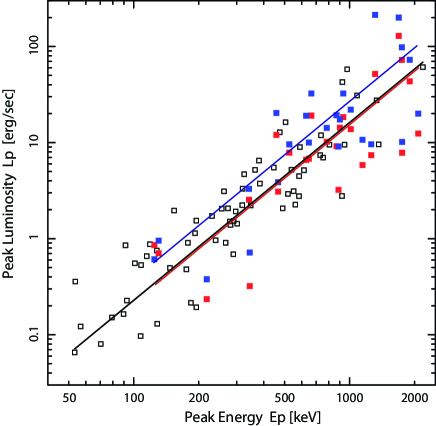
Figure 2: The $E_{p}$–$L_{p}$ distributions of Konus data. The blue and the red solid squares are the peak luminosity measured with 64 msec and 1024 msec time scale in the observer frame, respectively. The black open squares are the data 1-second (or 1024 msec) peak luminosity observed by the other missions. The black, red and blue solid lines are the best fit power-law functions for the same colour data with the fixed index, respectively. The blue data systematically distribute higher than the black line with the factor of 1.70. On the other hand, the red points are consistent with the black line.

In figure 2, we show the $E_{p}$–$L_{p}$ distributions of the Konus data. The blue and the red filled squares are the peak luminosity measured with 64 msec and 1024 msec time scale in the observer frame, respectively. The black open squares are the data of 1 second peak luminosity observed by the other missions. The black, red and blue solid lines are the best fit power-law functions for the same colour data with the fixed index, respectively. We can find that the blue solid line is apart from the other two lines, and the normalization of the blue line is 1.70 times higher than the black one. On the other hand, the red line is almost same as the black one with the factor of 0.96. This fact indicates that the 64 msec peak luminosity makes systematic dispersion in the $E_{p}$–$L_{p}$ correlation. Several past results, i.e. Nava et al. (2008); Ghirlanda et al. (2009) as well as our results by Kodama et al. (2008); Tsutsui et al. (2009), were argued about the selection effect and the GRB cosmology using the 64 msec peak luminosity for the Konus data. At present, since the number fraction of the Konus data is about 25 % of the entire 101 samples, the definition of the time scale should be treated correctly. Therefore the newly constructed database in this paper is more uniform compared with the past database, and appropriate to examine the origin of the data dispersion on the $E_{p}$–$L_{p}$ correlation.

The data are summarized in table Acknowledgments in appendix LABEL:sec:appendix. Additionally, we also show the data excluded from the database in table Acknowledgments and Acknowledgments because of several reasons. For example, we know that so-called low luminosity GRBs and outliers are really exist. In this paper, we call the data “outlier” which locates outside of the 3 $\sigma$ confidence region of the $E_{p}$–$L_{p}$ and the $E_{p}$–$E_{iso}$ correlations (see section 3). These groups are summarized in table Acknowledgments. In table Acknowledgments, we show several events with large ambiguity on the redshift and the spectral parameters. Several famous short GRBs are also listed in the same table as a reference, since their peak luminosity is determined by the millisecond time scale, and we can not convert them into the 1-second peak luminosity. In the following sections 3, we discuss the $E_{p}$–$L_{p}$ and $E_{p}$–$E_{\rm iso}$ correlation. After that, in section 4, we examine a flux dependence and an redshift evolution effect for these two correlations with table Acknowledgments.

3 Correlations

In figure 3, we show the $E_{p}$–$L_{p}$ (upper) and the $E_{p}$–$E_{\rm iso}$ (lower) correlations for all events listed in table Acknowledgments and table Acknowledgments. We used the equations 6 and 7 when we estimate the isotropic energy and the 1-second peak luminosity, respectively. The solid black straight lines are the best-fit power-law functions for good data listed in table Acknowledgments. The black curves around the straight lines represent 3 $\sigma$ statistical errors defined as,

$$\sigma_{\log{L_{p}(E_{\rm iso})}}=\sqrt{\sigma_{A}^{2}+\left(\sigma_{B}\log\left(\frac{E_{p}}{\rm 355~{}keV}\right)\right)^{2}},$$ (8)

where $\sigma_{A}$ and $\sigma_{B}$ are errors on the normalization and the power-law index when we express the correlation as $L_{p}({\rm or}~{}E_{iso})=AE_{p}^{B}$, respectively. The dotted lines are 3 $\sigma$ confidence regions including the data dispersion (systematic error).

In order to reduce the effect of samples which have unexpectedly large systematic error or which constitute different (unknown) family of GRBs, we have to identify and remove outliers. We identified the outliers as follows. First, we use all samples except the two low-luminosity GRBs and obtain a tentative best-fit relation. Then samples which are more than 3-sigma away from the tentative relation are removed and a new (and still tentative) best-fit relation is obtained. Performing these procedures iteratively, we finally obtain the true best-fit relation and outliers. Thus, the selection of the outliers is not arbitrary. As a result, we found 6 outliers, represented by the black points in figure 3.

Our method is similar to those adopted in the analyses of Type Ia SNe (e.g. Kowalski et al. (2008)) and Cepheid variables (e.g. Riess et al. (2009)). It may be instructive to note that the number fractions of outliers are about the same for GRBs, Type Ia SNe and Cepheid.

In figure 3, each color means the long GRBs (red points), high-redshift GRBs ($z>6$, blue points) and short GRBs (green points), respectively. Recently, Levesque et al. (2010) suggested a definition of short-hard/long-soft GRBs with a statistical method. Their definition is roughly (1) events with $T^{\rm obs}_{90}/(1+z)\leq 1.0$ sec are short-hard GRBs. (2) events with $T^{\rm obs}_{90}/(1+z)\geq 2.0$ sec are almost long-soft GRBs. (3) events with $1.0<T^{\rm obs}_{90}/(1+z)<2.0$ sec can not be clearly defined but events with $E_{p}^{\rm obs}>100~{}{\rm keV}$ and shorter time scale (close to $\sim 1~{}{\rm sec}$) are likely to be short-hard GRBs. Here, $T^{\rm obs}_{90}$ is measured as the time duration during the 90 % of total observed photons have been detected while the $T^{\rm obs}_{90}$ values highly depend on the energy band and the sensitivity of instruments. In this paper, we refer to their criteria while the original bimodal distribution of $T^{\rm obs}_{90}$ measured by BATSE (Fishman et al., 1994) is seen in the observer frame.

We estimated the best fit power-law function for the data listed in table Acknowledgments:

$$L_{p}=10^{52.43\pm 0.037}\times\left[\frac{E_{p}(1+z)}{355{\rm keV}}\right]^{1.60\pm 0.082},$$ (9)

$$E_{\rm iso}=10^{53.00\pm 0.045}\times\left[\frac{E_{p}(1+z)}{355{\rm keV}}\right]^{1.57\pm 0.099}.$$ (10)

Here we included not only the statistical errors but also the data dispersion (systematic error) with weighting factor when we estimated the best fit values and errors in these correlations. The data dispersions are estimated as $\sigma_{{\rm sys},\log L_{p}}=0.33$ for the $E_{p}$–$L_{p}$ correlation and $\sigma_{{\rm sys},\log E_{\rm iso}}=0.37$ for the $E_{p}$–$E_{\rm iso}$ correlation, respectively. Then, the correlation coefficients are 0.889 for 99 d.o.f for the $E_{p}$–$L_{p}$ correlation and 0.867 for 96 d.o.f for the $E_{p}$–$E_{\rm iso}$ correlation. These values correspond to the chance probability of $2.18\times 10^{-35}$ and $4.27\times 10^{-31}$, respectively.

The functional forms of these two correlations originally proposed in Yonetoku et al. (2004) and Amati et al. (2006) are

$$\frac{L_{p}}{10^{52}~{}{\rm erg~{}s^{-1}}} = (2.34^{+2.29}_{-1.76})\times 10^{-5}\Bigl{[}\frac{E_{p}}{1~{}{\rm keV}}\Bigr{]}^{2.0\pm 0.2},$$ (11)

$$\frac{E_{p}}{1~{}{\rm keV}} = (81\pm 2)\Bigl{[}\frac{E_{\rm iso}}{10^{52}~{}{\rm erg}}\Bigr{]}^{0.57\pm 0.02},$$ (12)

respectively. The power-law index of the revised $E_{p}$–$L_{p}$ correlation is slightly different from the original one, but consistent within 2 $\sigma$ confidence level. Considering that Yonetoku et al. (2004) were able to use only 16 samples, 2 $\sigma$ level agreement would not be strange. For the $E_{p}$–$E_{\rm iso}$ correlation, the power-law index of our result is consistent with the original one by Amati et al. (2006) within 1 $\sigma$ confidence level.

It is a hot topic whether the short GRBs are consistent with these correlations or not (Ghirlanda et al., 2009). In the criteria of short GRBs by Levesque et al. (2010), they are consistent with both correlations within the systematic error. However the number of short GRBs is still poor, so more future observations and arguments should be required.

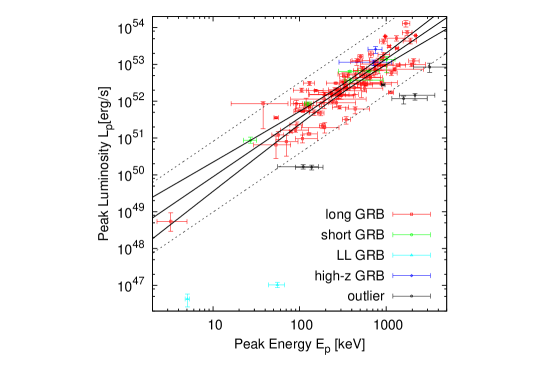
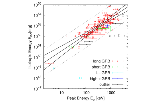
Figure 3: The $E_{p}$–$L_{p}$ correlation (top) and the $E_{p}$–$E_{\rm iso}$ correlation (bottom) for all events listed in table Acknowledgments and Acknowledgments. The red and green points indicate the data of long-GRBs and short-GRBs defined by Levesque et al. (2010) in the rest frame of GRBs. The 2 light-blue plots are the well-known low-luminosity GRBs of GRB 980425 and GRB 060218. The blue points are high-redshift GRBs with $z>6$ (GRB 080913, GRB 090423). The solid black straight lines are the best fit function for long (red) and short (green) GRBs while two black curves around the straight line are 3 $\sigma$ statistical error. The dotted lines are 3 $\sigma$ systematic errors in equations 9 and 10. The 6 black plots are outliers which locates beyond 3 $\sigma$ confidence region from the best fit function of the $E_{p}$–$L_{p}$ and/or the $E_{p}$–$E_{\rm iso}$ correlations (GRB 050223, 050803, 050904, 070714B, 090418, and 091003).

4 Possible Origin of Data Dispersion

As shown in the previous section, the two correlations are very tight, although there are some dispersion around the best-fit correlation: $\sigma_{{\rm sys},\log L_{p}}=0.33$ and $\sigma_{{\rm sys},\log E_{\rm iso}}=0.37$, respectively. These correspond to the errors of about factor 2 when we estimate $L_{p}$ and $E_{\rm iso}$ from $E_{p}$.

One may wonder if these correlations represent the intrinsic property of GRBs or just come from the truncation effect of the detector threshold (Butler et al., 2007; Shahmoradi & Nemiroff, 2009). In figure 4, we show the sample distributions in observer-frame quantities ($E_{p}^{\rm obs}$–$F_{p,{\rm bol}}$ plane and $E_{p}^{\rm obs}$–$S_{\rm bol}$ plane). We can see some correlations over three orders of magnitude in the observed brightness range, but these are substantially affected by the truncation of samples due to the detector sensitivity. In particular, GRBs with low brightness and large $E_{p}^{\rm obs}$ are generally hard to observe. Some authors insist that the truncation effect create the apparent correlations in GRB frame, such as the $E_{p}$–$L_{p}$ and $E_{p}$–$E_{\rm iso}$ correlations.

However, this is not the case as we show. We divide the GRB events into three groups according to their brightness as shown in figure 4 and table 2 (for the details of the classification see the next subsection). As one can see, each group does not show significant correlation in the observer frame and it is evident that the truncation effect would be very small within each group. However, as figure 5 shows, each group shows a clear correlation in GRB frame. Thus, we can conclude that the correlations in GRB frame are not caused by the truncation effect.

In this section, we seek for the origin of the dispersion of the correlations. The dispersion may be intrinsic and cannot be reduced, or some unknown systematic errors may contribute to the dispersion. Specifically we study the flux/fluence dependence and redshift evolution of the correlations and estimate the systematic errors accompanying them.

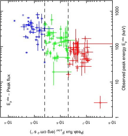
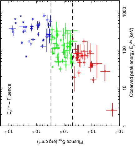
Figure 4: The observed $E_{p}$–$F_{p,{\rm bol}}$ (left) and the $E_{p}$–$S_{\rm bol}$ (right) correlations. We classified the entire data into three groups according to each brightness range as listed in table 2. Each three group does not show the strong correlation between $E_{p}$ and brightness, while the entire data set shows the clear correlation because of the truncation effect by the detector threshold. If each group consists of each $E_{p}$–$L_{p}$ and $E_{p}$–$E_{\rm iso}$ relation, then we may conclude the both correlations are real, and not due to the truncation effect.

4.1 Brightness Dependence

Here we test the brightness dependence of the correlations using our database listed in table Acknowledgments. The database consists of events with various brightness. The brightest event is GRB 991216 with the peak flux of $F_{\rm p,bol}=5.80\times 10^{-5}~{}{\rm erg~{}cm^{-2}s^{-1}}$, while the dimmest one is GRB 020903 with the peak flux of $F_{\rm p,bol}=2.94\times 10^{-8}~{}{\rm erg~{}cm^{-2}s^{-1}}$. The difference is about 3 orders of magnitude. If the $E_{p}$–$L_{p}$ and the $E_{p}$–$E_{\rm iso}$ correlations are affected by the detector sensitivity as suggested by Butler et al. (2007), systematic difference according to the brightness would be seen in the distribution of events on $(E_{p},L_{p})$ and $(E_{p},E_{\rm iso})$ planes.

We classify GRB events into three groups according to the bolometric peak flux to discuss the flux dependence of the $E_{p}$–$L_{p}$ correlation, as shown in table 2: 30 events with $F_{\rm p,bol}<5\times 10^{-7}$ (dim class), 41 events with $5\times 10^{-7}\leq F_{\rm p,bol}\leq 4\times 10^{-6}$ (middle class), and 30 events with $F_{\rm p,bol}>4\times 10^{-6}$ (bright class). We derive $E_{p}$–$L_{p}$ correlation for each group and investigate whether they are consistent with each other. We perform a similar analysis for the $E_{p}$–$E_{\rm iso}$ correlation considering three groups according to the bolometric fluence: 27 events with $S_{\rm bol}<5\times 10^{-6}$ (dim class), 41 events with $5\times 10^{-5}\leq S_{\rm bol}\leq 3\times 10^{-4}$ (middle class), 30 events with $S_{\rm bol}>3\times 10^{-5}$ (bright class) as shown in table 2.

In figure 5 (top left and right), we show the $E_{p}$–$L_{p}$ and the $E_{p}$–$E_{\rm iso}$ correlations for three brightness classes. The red, green and blue points represent the dim, middle and bright class as described in table 2, respectively. We adopt the power-law model for each group, and estimate the best fit function as well as the data dispersions of $\sigma_{{\rm sys},\log L_{p}}$ and $\sigma_{{\rm sys},\log E_{\rm iso}}$, respectively. The solid line and curves for each colour mean the best-fit function and 3 $\sigma$ statistical boundary lines as same in figure 3. The results are summarized in table 1.

In figure 5 (bottom left and right), we also show the 2 $\sigma$ acceptable regions for three groups. For the $E_{p}$–$L_{p}$ correlation, we can recognize that three best fit lines are overlapping. So we can say that the peak-flux dependence is not significant in the $E_{p}$–$L_{p}$ correlation. By contrast, for the $E_{p}$–$E_{\rm iso}$ correlation, we found a weak trend that the events with larger fluence have the larger $E_{\rm iso}$ (or smaller $E_{p}$).

The discrepancy between the bright and dim classes is over 2 $\sigma$ statistical level and would contribute to the dispersion in the $E_{p}$–$E_{\rm iso}$ correlation. One should notice that the discrepancy is only a factor of 2 or 3, while the correlation itself covers beyond 3 or 4 orders of magnitude in the $E_{\rm iso}$ range. Therefore the detector sensitivity would contribute to the data dispersion of the $E_{p}$–$E_{\rm iso}$ correlation, but not affect the argument on the existence of the correlation itself. We give an interpretation of this dependence in section 5. It should be noted that, as we pointed out in section 1, the flux/fluence dependence of the correlations can be regarded as an estimator for the systematic error due to the threshold effect.

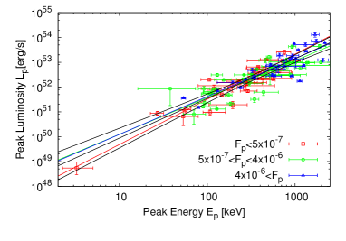
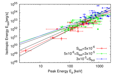
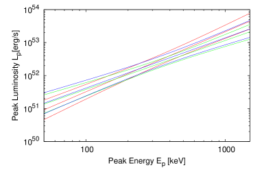
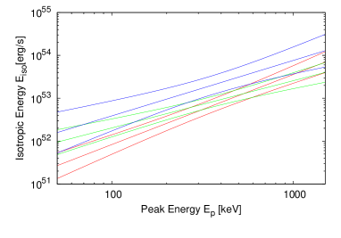
Figure 5: (Top) The left and right panels show the $E_{p}$–$L_{p}$ correlation and the $E_{p}$–$E_{\rm iso}$ correlation in the three flux (fluence) ranges listed in table 2. Red, green and blue points represent dim, middle and bright classes, respectively. The black line and curves are the best-fit function and 3 $\sigma$ statistical error derived in section 3 (see equations 9 and 10). (Bottom) The left and right panels show 2 $\sigma$ statistical error regions around the best fit functions of the $E_{p}$–$L_{p}$ and $E_{p}$–$E_{\rm iso}$ correlations for the three flux (fluence) ranges listed in table 2. Each colour means the same of top panels. The black line and curves are the best-fit function and 2 $\sigma$ statistical error derived in section 3. The $E_{p}$–$L_{p}$ correlation is consistent with each other in 1 $\sigma$ statistics while the $E_{p}$–$E_{\rm iso}$ correlation show difference with 2 $\sigma$ confidence level.

4.2 Redshift Dependence

We also examine the redshift dependence of the $E_{p}$–$L_{p}$ and the $E_{p}$–$E_{\rm iso}$ correlations. This is a critical issue when we use these empirical correlations as cosmological tools like Type Ia supernovae. Our database covers a wide redshift range of $0.168\leq z\leq 8.2$ and we divide the samples into three classes; 31 GRBs with $z<1$, 36 GRBs with $1<z<2.5$, and 35 GRBs with $z>2.5$. In figure 6, we show the $E_{p}$–$L_{p}$ (upper left) and the $E_{p}$–$E_{\rm iso}$ (upper right) correlations of each class. The best-fit results and 1 $\sigma$ statistical errors are summarized in table 3. The 2 $\sigma$ confidence regions for three classes are also shown in the bottom left and right panels in figure 6, respectively. The meaning of each solid line is the same as one of figure 5.

A difference between high- and low-redshift classes can be seen in the $E_{p}$–$L_{p}$ correlation at 2 $\sigma$ level, and a systematic redshift dependence is also seen in the power-law index. Especially the discrepancy is remarkable toward higher value of $E_{p}$ and $L_{p}$. By contrast, in the $E_{p}$–$E_{\rm iso}$ correlation, the three classes are consistent at 1 $\sigma$ level through the entire correlations.

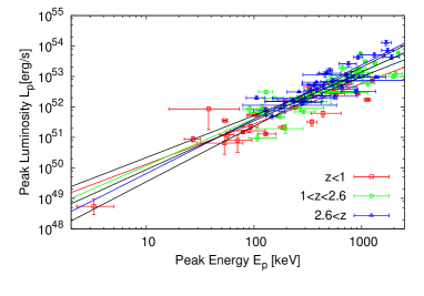
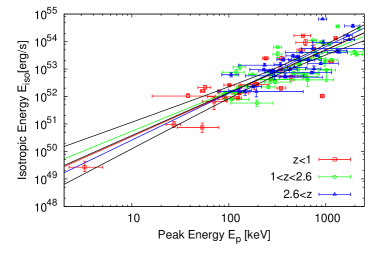
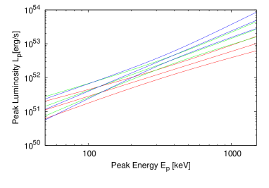
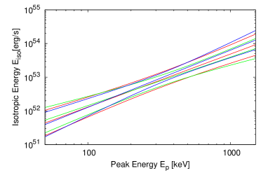
Figure 6: (Top) The left and right panels show the $E_{p}$–$L_{p}$ correlation and the $E_{p}$–$E_{\rm iso}$ correlation in the three redshift ranges. Each colour represents $z<1$ (red), $1<z<2.5$ (green) and $z>2.5$ (blue), respectively. The black line and curves are best-fit function and 3 $\sigma$ statistical error derived in section 3. (Bottom) The left and right panels show 2 $\sigma$ statistical error regions around the best-fit functions of the $E_{p}$–$L_{p}$ and $E_{p}$–$E_{\rm iso}$ correlations in the three redshift ranges. Each colour means the same of top panels. The black line and curves are best-fit function and 2 $\sigma$ statistical error derived in section 3. The $E_{p}$–$E_{iso}$ correlation is consistent with each other in 1 $\sigma$ statistics while the $E_{p}$–$L_{p}$ correlation show difference with 2 $\sigma$ confidence level.

5 Discussion and Summary

In this paper, combining data from multiple detectors and recalculating the peak flux for Konus events, we constructed a uniform database of GRBs with known redshift and well-observed spectral quantities to determine $E_{p}$, $L_{p}$ and $E_{\rm iso}$. The 101 GRB samples enabled us to derive the $E_{p}$–$L_{p}$ and $E_{p}$–$E_{\rm iso}$ correlations with small statistical errors compared with their dispersions. By dividing the samples according to the observed flux/fluence and showing the correlation of each group, it was shown that the correlations are intrinsic to GRBs and not due to the truncation effect of the detector threshold. Then we examined the flux/fluence dependence and redshift evolution of the correlations, which is a crucial issue when we use GRBs as cosmological tools. We found a fluence-dependence in the $E_{p}$–$E_{\rm iso}$ correlation, and a redshift dependence in the $E_{p}$–$L_{p}$ correlation. Both dependences are about 2 $\sigma$ statistical level and relatively weak so that they could still be used as cosmological tools. However, they would contribute to the data dispersion in the correlations.

Let us give some comments on the work by Butler et al. (2007). They suggested, using the Swift data, the $E_{p}$–$E_{\rm iso}$ correlation is due to the detector threshold. The $E^{\rm obs}_{p}$ value of many Swift events can not be determined by the observational data because of the narrow energy range of BAT instrument. So, using Bayesian statistics approach, they estimated the $E^{\rm obs}_{p}$ values for 218 events based on a parent distribution of spectral parameters suggested by BATSE data (Preece et al., 2000). Butler et al. (2007) found a pseudo $E_{p}$–$E_{\rm iso}$ correlation which is inconsistent with the original one by Amati et al. (2002). They claimed that this inconsistency is caused by the large intrinsic scatter of the correlation. In other words, the “tight” $E_{p}$–$E_{\rm iso}$ correlation is an artifact result, because almost all dimmer samples close to the detector sensitivity would be outliers of the $E_{p}$–$E_{\rm iso}$ correlation by Amati et al. (2002). However we need caution to compare their work with others, because their $E_{p}^{\rm obs}$ values are just estimated by the Bayesian statistics approach, and not observed. These simulated $E_{p}^{\rm obs}$ values highly depend on the assumed parent distribution of spectral parameters. Our approach to prove the existence of the correlation is very different from this approach. We do not assume anything about the statistical property of GRB samples.

The fluence dependence in the $E_{p}$–$E_{\rm iso}$ correlation may be consistent with the conclusion by Nava et al. (2008), although the statistical significance is only 2 $\sigma$ level. This dependence might be interpreted as follows. We can observe only bright parts in the lightcurve for dim GRBs and tend to underestimate their total energies. In other words, the dispersion of the $E_{p}$–$E_{\rm iso}$ correlation might be influenced by the instrumental threshold effect because the dimmer events can be observed only for the more sensitive instruments. In contrast, this effect would not be expected for the $E_{p}$–$L_{p}$ correlation because it involves the peak luminosity ($L_{p}$) which is determined only by the brightest part of each event.

We also found a weak redshift dependence in the $E_{p}$–$L_{p}$ correlation. Of course, one interprets that this dependence is the intrinsic property of GRBs. However, let us point out a possibility of systematic overestimation of the peak luminosity $L_{p}$ for high-redshift GRBs. In the $E_{p}$–$L_{p}$ correlation, we usually use 1 second peak flux in the observer frame when we estimate $L_{p}$. However this means that the time scale of peak luminosity $L_{p}$ in the GRB frame depends on the redshift because of the cosmological time dilation. In other words, the time scale in the GRB frame becomes shorter for higher-redshift GRBs. In general, we can expect the peak luminosity increases as the time scale becomes shorter as shown in figure 1. For example, considering a GRB at $z=4$, the observed 1 second peak flux corresponds to the 200 msec one at the GRB frame. According to figure 1, in this case, we systematically overestimate the peak luminosity about 30–50 % on average.

Thus, difference in the time interval in the GRB frame would induce a systematic error in $L_{p}$. This effect would make high-redshift GRBs look systematically brighter than low-redshift GRBs and may result in the apparent redshift dependence suggested in figure 6. Therefore, the redshift dependence of the $E_{p}$–$L_{p}$ correlation might be understood as a selection bias due to the inappropriate definition of $L_{p}$, rather than an intrinsic property of GRBs. If this argument is true, we may enable to reduce the systematic errors of $E_{p}$–$L_{p}$ correlation when we use the same time scale in each GRB frame. Then we will make the $E_{p}$–$L_{p}$ correlation more accurate luminosity indicator. This will be presented elsewhere in near future.