Convective Babcock-Leighton Dynamo Models

Abstract

We present the first global, three-dimensional simulations of solar/stellar convection that take into account the influence of magnetic flux emergence by means of the Babcock-Leighton (BL) mechanism. We have shown that the inclusion of a BL poloidal source term in a convection simulation can promote cyclic activity in an otherwise steady dynamo. Some cycle properties are reminiscent of solar observations, such as the equatorward propagation of toroidal flux near the base of the convection zone. However, the cycle period in this young sun (rotating three times faster than the solar rate) is very short ($\sim$ 6 months) and it is unclear whether much longer cycles may be achieved within this modeling framework, given the high efficiency of field generation and transport by the convection. Even so, the incorporation of mean-field parameterizations in 3D convection simulations to account for elusive processes such as flux emergence may well prove useful in the future modeling of solar and stellar activity cycles.

1. Introduction

The emergence of magnetic flux through the solar photosphere regulates solar variability and powers space weather. It is clear that this flux originates in the solar interior and is produced by the solar dynamo. However, it is currently unclear what role flux emergence plays in establishing the 22-year solar activity cycle. Is it an essential ingredient or merely a superficial by-product of deeper-seated dynamics?

One of the principle means by which flux emergence may act an an essential ingredient in the operation of the solar dynamo is through the so-called Babcock-Leighton (BL) mechanism (Babcock, 1961; Leighton, 1964). The BL mechanism arises through the dynamics of flux emergence. As a buoyant flux tube rises through the convection zone, the Coriolis force induces a twist in the axis of the tube that is manifested upon emergence as a poleward displacement between the trailing and leading edges of a bipolar active region. When the active region subsequently fragments and disperses due to surface convection and meridional flow, the redistribution of vertical flux induces a net electromotive force (emf) that converts mean toroidal field to poloidal field. Although doubts remain about the viability of the BL mechanism as the principle source of poloidal flux, its empirical foundation and robustness have made it an integral element in many recent mean-field dynamo models of the solar cycle (reviewed by Dikpati & Gilman, 2009; Charbonneau, 2010).

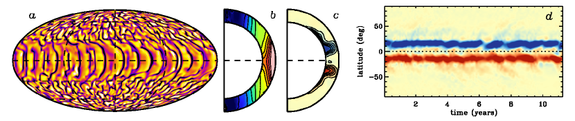
Figure 1.— Progenitor simulation, Case D3, from Brown et al. (2010). ($a$) Radial velocity in a Mollweide projection near the top of the computational domain ($r=0.953R$, $t=2$ yr, color table saturation $\pm$ 70 m s^-1, yellow/orange upflow, blue/black downflow). ($b$) Angular velocity $\Omega/2\pi$, averaged over 1200 days (7.8-11.3 yrs, saturation 1140–1320 nHz, white/red fast, blue/black slow). ($c$) Mean toroidal magnetic field $\left<B_{\phi}\right>$ averaged over longitude and time (15 day average near $t=2$ yrs, saturation $\pm$ 8 kG, red positive, blue negative). ($d$) $\left<B_{\phi}\right>$ in the mid convection zone ($r=0.84R$) versus latitude and time (colors as in $c$, saturation $\pm$ 4 kG).

Current simulations of global solar and stellar convection do exhibit sustained dynamo action and, depending on the parameter regime, can produce magnetic cycles (Ghizaru et al., 2010; Racine et al., 2011; Brown et al., 2011). Yet, these simulations do not have sufficient resolution to reliably capture flux emergence or the BL mechanism. Nelson et al. (2011) recently reported the first convective dynamo simulation to exhibit the spontaneous, self-consistent generation of buoyant magnetic flux structures generated by convectively-driven rotational shear. However, even these cannot realistically simulate the subtle, multi-scale dynamics of flux emergence and dispersal that underlies the BL mechanism. This would require (1) very low diffusion to form concentrated flux structures, (2) very high resolution to capture the destabilization and coherent rise of those structures, and (3) a realistic depiction of surface convection, meridional flow, and radiative transfer in order to capture the emergence, coalescence, fragmentation, and dispersal of bipolar active regions (Cheung et al., 2010). Each of these is a formidable computational challenge in its own right, stetching the limits of modern supercomputers. No global model is capable of unifying convective dynamos and the BL mechanism through direct numerical simulation.

Thus, the presence of magnetic cycles in global convection simulations demonstrates that the BL mechanism is not a necessary ingredient for cyclic activity. How this may or may not apply to the solar dynamo is a complex, unresolved issue and we make no attempt at a comprehensive discussion here. Our purpose is rather to investigate how flux emergence may alter the behavior of a convective dynamo by means of the BL mechanism. The BL mechanism is modeled using a mean-field parameterization intended to mimic dynamics that cannot be explicitly captured by the simulation itself for the reasons outlined above. Our approach is described in §2 and simulation results are presented in §3, along with interpretive discussion.

Before proceeding, it is worth emphasizing up front that the simulations we consider here are of a solar-like star rotating three times more rapidly than the Sun (3$\Omega_{\odot}$). This is done because it is a tidy numerical experiment; without BL forcing, this dynamo builds strong large-scale fields that do not undergo cycles. Other parameter regimes, including those at the solar rotation rate, will be considered in future work.

2. Model

The starting point for our investigation is the convective dynamo simulation that we refer to as case D3 and that is described in detail by Brown et al. (2010). We refer the reader to that paper for further information on the set up and results of the simulation as well as the ASH (Anelastic Spherical Harmonic) code that is used to solve the equations of magnetohydrodynamics (MHD) in a rotating spherical shell under the anelastic approximation. Solar values are used for the luminosity and the background stratification but the rotation rate is a factor of three faster than the Sun, as mentioned above. The spatial resolution of all simulations reported in this paper is 96 $\times$ 256 $\times$ 512 ($r$, $\theta$, $\phi$). The simulation domain spans from $r_{1}=0.718R$ to $r_{2}=0.966R$, where $R$ is the solar radius.

The salient feature of Case D3 that we are interested in here is the presence of persistent toroidal field structures that we term magnetic wreaths. The convection exhibits an intricate, evolving small-scale structure (Fig. 1$a$) but produces a substantial differential rotation (Fig. 1$b$) that in turn promotes the generation of prominent magnetic wreaths (Fig. 1$c$). The mean toroidal field is approximately symmetric about the equator, with one wreath in each hemisphere of opposite polarity. Although continual buffeting by convective motions induces non-axisymmetric and temporal fluctuations, the mean field is remarkably persistent, retaining its essential structure indefinitely (Fig. 1$d$). After they are established, the wreaths persist for at least 60 years (the duration of the simulation) with no sign of abating (Brown et al., 2010). This time interval is much longer than the rotation period (9.3 days), the convective turnover time scale (about 20 days) and the ohmic diffusion time (about 3.6 years).

The simulations described in this paper are all restarted from the same iteration of Case D3, defined as time $t=0$. This includes the unmodified D3 run shown in Figure 1, which was continued beyond the restart iteration for comparison purposes. The absence of initial transients in Fig. 1 demonstrates that this simulation has reached a statistically steady state by the mutual reference time $t=0$.

The anelastic MHD equations for the conservation of mass, momentum, and thermal energy are solved with no modification. The only difference between the simulations presented here and that presented in Brown et al. (2010) is in the magnetic induction equation where we add an additional poloidal source term $S(r,\theta)$ as follows:

$$\frac{\partial{\bf B}}{\partial t}=\mbox{\boldmath$\nabla\times$}\left({\bf v}\mbox{\boldmath$\times$}{\bf B}-\eta\mbox{\boldmath$\nabla\times$}{\bf B}+S\mbox{\boldmath$\hat{\phi}$}\right)$$ (1)

The additional term is intended to mimic the generation of mean poloidal field by the BL mechanism. Following the mean-field BL dynamo model of Rempel (2006), we choose

$$S(r,\theta)=\alpha f(r)g(\theta)\hat{B}_{\phi}$$ (2)

where $f(r)$ and $g(\theta)$ are radial and latitudinal profiles

$$f(r)=\mbox{max}\left[0,1-\frac{(r-r_{2})^{2}}{d^{2}}\right]$$ (3)

$$g(\theta)=\frac{3\sqrt{3}}{2}~{}\sin^{2}\theta\cos\theta$$ (4)

and $\hat{B}_{\phi}$ is a measure of the mean toroidal flux at the base of the convection zone

$$\hat{B}_{\phi}=\int_{r_{1}}^{r_{b}}h(r)\left<B_{\phi}\right>dr~{}~{}~{}.$$ (5)

Brackets $<>$ denote an average over longitude and $h$ is an averaging kernal given by $h(r)=h_{0}\left(r-r_{1}\right)\left(r_{b}-r\right)$. The integration is confined to a region near the base of the convection zone, below $r_{b}=0.79R$ and the normalization $h_{0}$ is defined such that $\int_{r_{1}}^{r_{b}}h(r)dr=1$.

Note that the radial profile in equation (3) is nonzero only near the top of the convection zone, for $r>r_{2}-d$. We choose $d=20$ Mm so the poloidal source operates above $r=0.937R$. Thus, the BL term is nonlocal in the sense that the poloidal source near the surface is proportional to the mean toroidal flux near the base of the convection zone. This is typical of BL dynamo models (e.g. Rempel, 2006).

The amplitude of the BL term, $\alpha$, includes an algebraic quenching of the form $\alpha=\alpha_{0}(1+B_{t}^{2}/B_{q}^{2})^{-1}$ where $B_{q}=1$ MG is the quenching field strength and $B_{t}^{2}=(1/2)\int_{0}^{\pi}\hat{B}^{2}\sin\theta d\theta$. In practice the fields generated are much less than $B_{q}$ so the quenching plays little role.

The magnetic diffusivity $\eta$ in all simulations is the same as in Case D3, varying from 1.56-7.69 $\times 10^{12}$ cm² s^-1 from the bottom to the top of the convection zone, $\propto\overline{\rho}^{-1/2}$, where $\overline{\rho}$ is the background density.

The objective of this paper is to vary the amplitude of the BL term $\alpha_{0}$ in order to investigate how flux emergence may alter the nature of the dynamo. We emphasize again that the 3D MHD equations are unmodified apart from the $S(r,\theta)$ term in eq. (1) so setting $\alpha_{0}=0$ reproduces Case D3 as shown in Figure 1 and as described at length in Brown et al. (2010).

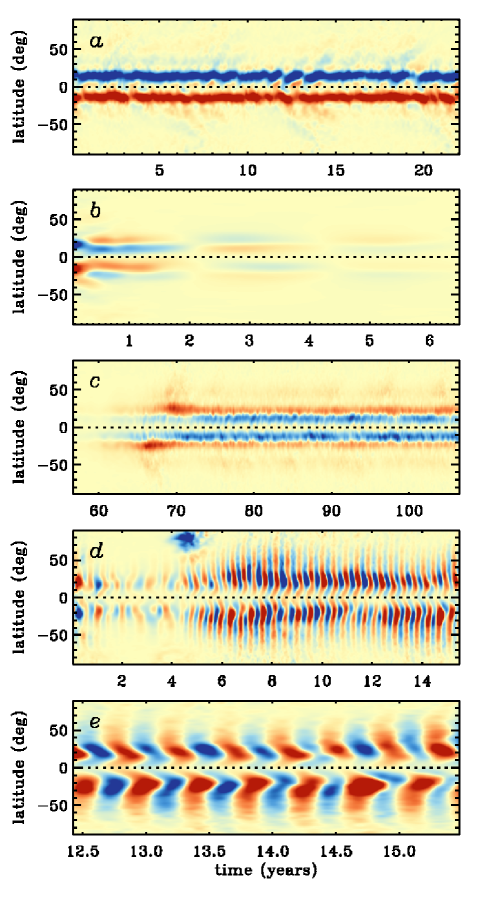
Figure 2.— Mean toroidal field as a function of latitude and time as in Fig. 1$d$ (same radial level, color scale, saturation $\pm$ 4 kG) with ($a$) $\alpha_{0}=$ 1 m s^-1, ($b$, $c$) $\alpha_{0}=$ 10 m s^-1, and ($d$, $e$) $\alpha_{0}=$ 100 m s^-1. Frame ($c$) represents a continuation of frame ($b$) at much later times. Frame ($e$) is a zoomed-in portion of frame ($d$) highlighting the magnetic cycles.

3. Results

Figure 2 shows “butterfly” diagrams (latitude-time plots of the mean toroidal field near the base of the convection zone) for a series of simulations with progressively increasing values of the BL forcing amplitude $\alpha_{0}$. For $\alpha_{0}=$ 1 m s^-1 the BL term is too weak to sigificantly influence the operation of the dynamo (Fig. 2$a$). The axisymmteric component of the poloidal field near the surface does increase but not enough to effect the maintenance of persistent wreaths in the lower convection zone.

For $\alpha_{0}=$ 10 m s^-1 the results are very different. The wreaths essentially vanish within a few years of simulation time (Fig. 2$b$). This can be attributed to the differential rotation operating on the mean poloidal field generated by the BL mechanism via the $\Omega$-effect. The sense of the poloidal field produced by the BL term is such that the $\Omega$-effect generates toroidal flux in the upper convection zone that is of opposite polarity to the sense of the wreaths. Convection rapidly mixes this flux, bringing together opposite polarities that are annihilated through ohmic dissipation. The magnetic energy in the mean fields drops rapidly, decaying by a factor of 10⁶ by $t\sim$ 30 yrs.

Yet, beyond about 30 years, the magnetic energy begins to rise again and the dynamo is reborn, saturating by about $t\sim$ 75 yrs (Fig. 2$c$) with a very different structure. Persistent toroidal wreaths are again present but they are symmetric about the equator, with two wreaths per hemisphere and a somewhat lower magnetic energy (about 27% less than in Case D3).

Increasing $\alpha_{0}$ by another order of magnitude produces prominent magnetic cycles (Fig. 2$d$). Toroidal wreaths form at mid latitudes in each hemisphere and propagate toward the equator, reminiscent of the solar butterfy diagram (Fig. 2$e$). However, the cycle period is much shorter than in the Sun; about 6 months compared to 22 years. Nonlinear modulation of the cycle is evident, with waxing and waning amplitudes and transient, weaker substructure in the butterfly diagram near the equator.

It is clear from Fig. 2$e$ that reversals in the two hemispheres are not precisely sychronized. A more careful analysis reveals that the phase difference shifts over time, suggesting that the two hemispheres are to some extent decoupled. For example, the northern hemisphere leads the southern hemisphere from $t\sim$ 4.5 – 11.5 yrs but the reverse is true for $t\sim$ 12 – 14.5 yrs. Similar shifts in the hemispheric phase difference (albeit less pronounced) have been reported in sunspot records; in particular, the southern hemisphere was apparently leading in cycles 18-20 while the northern was leading in cycles 21-23 (McIntosh et al., 2012).

Figure 3.— Parity of the mean toroidal field as a function of time for the simulation shown in Fig. 2$d$,$e$ ($\alpha_{0}=$ 100 m s^-1).

The symmetry of the dynamo about the equator can be quantified by the parity ${\cal P}=(B_{s}^{2}-B_{a}^{2})/(B_{s}^{2}+B_{a}^{2})$, where $B_{s}$ and $B_{a}$ are the symmetric and antisymmtric components of $\left<B_{\phi}\right>$ respectively (sampled at $r=0.84R$). The parity of Case D3 and for $\alpha_{0}=$ 1 m s^-1 ranges between -0.5 and -1 while that for $\alpha_{0}$ = 10 m s^-1 ranges between positive 0.5-1. By contrast, the cyclic dynamo ($\alpha_{0}=$ 100 m s^-1) shifts between positive and negative parity as time proceeds. It does not exhibit the high synchronization of the solar cycle which exhibits a persistent negative parity.

As expected, the addition of a BL term has a substantial influence on the amplitude and structure of the mean poloidal field. Without it, the poloidal field has a roughly octupolar structure, such that $\left<B_{r}\right>$ is radially outward near the north pole, inward near the core of the northern wreath, and antisymmetric about the equator (Brown et al., 2010). As noted above, the BL term generates opposing poloidal flux at mid-latitudes near the surface, producing multi-polar structure and enhancing dissipation. This plays an essential role in establishing the cycles of Fig 2$d$-$e$ and is evident in movies of the mean-field evolution. The typical amplitude of the mean poloidal field near the surface for $\alpha_{0}=100$ m s^-1, 1-2 kG, is much larger than for $\alpha_{0}=0$ ($\sim$ 200 G in Case D3) but the overall (3D) magnetic energy is about a factor of two smaller.

The transition from steady to cyclic dynamos occurs when the BL term $S$ competes with the fluctuating emf $\left<{\bf v}^{\prime}\mbox{\boldmath$\times$}{\bf B}^{\prime}\right>$, where ${\bf v}^{\prime}={\bf v}-\left<{\bf v}\right>$ and ${\bf B}^{\prime}={\bf B}-\left<{\bf B}\right>$. This in turn occurs when $\alpha_{0}$ becomes comparable to the velocity of the convective motions, $V_{c}$. The relevant scale for $V_{c}$ is the rms value of the meridional components of ${\bf v}^{\prime}$, which is about 120 m s^-1 near the top of the convection zone in Case D3, decreasing with depth.

A legitimate question is whether the cyclic dynamo in Fig. 2$d$,$e$ is operating in an essentially mean-field, axisymmteric mode. In other words, if the BL term were to dominate the generation of mean poloidal field and the differential rotation were to dominate the generation of mean toroidal field via the $\Omega$-effect, then one might expect this 3D simulation to behave very similarly to an analogous, axisymmetric mean-field model. Under this mean-field scenario, coupling between the poloidal and toroidal source regions might occur through the nonlocality of the BL term, the mean meridional flow, and the turbulent diffusion $\eta$. The primary role of the resolved convective motions would then be to maintain the mean flows.

In order to assess whether this mean-field scenario is indeed a valid interpretation of the cyclic activity shown in Fig. 2$d$,$e$, we have initiated another simulation in which we have artificially suppressed the fluctuating emf. More specifically, we have replaced the ${\bf v}\mbox{\boldmath$\times$}{\bf B}$ term in equation (1) with only mean-field induction $\left<{\bf v}\right>\mbox{\boldmath$\times$}\left<{\bf B}\right>$. This simulation was restarted from that shown in Fig. 2$d$,$e$ at $t=8.25$ yrs with the same parameters. The only difference is the absence of the fluctuating emf.

The dynamo mode changes dramatically, as demonstrated in Fig. 4. The non-axisymmetric magnetic field is quickly dissipated by ohmic diffusion, with the corresponding energy decreasing by six orders of magnitude within two years (shear promotes more rapid dissipation than the nominal 3.6 year diffusion time scale). The total magnetic energy is about a factor of three larger than in the progenitor simulation of Fig. 2$d$,$e$ and is dominated by a strong, axisymmtric toroidal field that is symmetric about the equator (positive parity) and reverses cyclically with a period of about 1.3 yrs. The butterfly diagram in Fig. 4 suggests poleward propagation but closer inspection of the mean field evolution reveals a dynamo wave that propagates toward the rotation axis, with a cylindrical orientation for the wave front. This is consistent with the cylindrical nature of the differential rotation profile (Fig. 1$b$) but is strikingly different from the progenitor simulation in Fig. 2$d$,$e$ which exhibits virtually no mean toroidal field at the equator even when the parity is positive. In short, cycles are longer, stronger, and less solar-like without a turbulent emf.

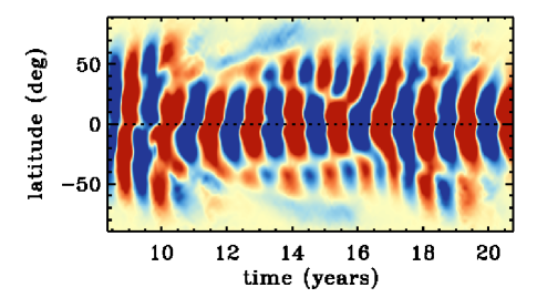
Figure 4.— Mean toroidal field versus latitude and time as in Fig. 2 (same radial level, color table, saturation $\pm$ 4kG) for a simulation with $\alpha_{0}=$ 100 m s^-1, along with an artificial suppression of the fluctuating emf $\left<{\bf v}^{\prime}\mbox{\boldmath$\times$}{\bf B}^{\prime}\right>$ (see text). Compare with Fig. 2$d$,$e$.

Thus, the cyclic dynamo in Fig. 2$d$,$e$ is not operating as a mean-field dynamo, or at least not in a naive sense. Convection contributes mean field generation and transport that plays an essential role in shaping the dynamo even for $\alpha_{0}$ as high as 100 m s^-1. Parity selection in cyclic dynamos is a subtle issue and space limitations preclude a thorough discussion here. We only remark that mean-field BL models have demonstrated that the relatively homogeneous nature of turbulent pumping (Guerrero & de Gouveia Dal Pino, 2008), the antisymmetric structure of a supplementary $\alpha$-effect operating near the base of the convection zone (Dikpati & Gilman, 2001), and efficient turbulent mixing that peaks in the upper convection zone (Hotta & Yokoyama, 2010) can all help promote negative (dipolar) parity. These mean-field results are loosely consistent with the 3D convection simulations reported here but warrant a more careful investigation which we reserve for future work.

In summary, we have shown that flux emergence can promote cyclic magnetic activity in a convective dynamo by means of the Babcock-Leighton mechanism. Although this result is to some extent anticipated by mean-field dynamo models, we have demonstrated it for the first time in a global convection simulation. The BL mechanism is not required to achieve cycles in convective dynamo simulations but, as we have shown here, it may help shape cycle properties such as the period, amplitude, and equatorward propagation of toroidal flux.

However, achieving cyclic activity through the BL mechanism is not easy. To make a significant impact on the dynamo, the amplitude of the BL $\alpha$-effect must be comparable to the convective velocity, $V_{c}$. In particular, we find that $\alpha_{0}>$ 10 m s^-1 is required to induce cyclic activity when $V_{c}\sim$ 100 m s^-1 in the upper convection zone. By comparison, typical values of $\alpha$ used in mean-field BL dynamo models of the solar cycle are less than 1 m s^-1 (e.g. Dikpati & Gilman, 2009; Charbonneau, 2010).

The relatively large value of $\alpha_{0}$ used here, together with the strong shear $|\mbox{\boldmath$\nabla$}\Omega|$ and the efficiency of convective transport, can likely account for the very short cycle period in this young, rapidly-rotating Sun ($\Omega=3\Omega_{\odot}$). Might other parameters produce a 22-yr period comparable to the solar cycle? This remains to be seen. Whether the cycle period is regulated by a dynamo wave or flux transport, the large value of $\alpha_{0}$ needed to promote cyclic activity ($>10$ m s^-1) and the short convective turnover time scale ($\sim$ 20 days) may favor relatively short cycle periods. Longer cycle periods can generally be achieved in mean-field BL dynamo models by reducing the efficiency of poloidal flux transport (e.g Dikpati & Gilman, 2009; Charbonneau, 2010) but we do not have that freedom here. Here the efficiency of transport is set by the convection, which in turn is an output of the simulation, regulated mainly by factors such as the stellar mass and luminosity that are set by observations. This implies either that the mean field generation and transport by solar convection is much less efficient than in the models considered here (due possibly to dynamical quenching of the turbulent $\alpha$ and $\beta$-effects or overestimation of the convective velocity), or that the solar dynamo does not adhere to a simple BL paradigm.

References

- Babcock (1961) Babcock, H. W. 1961, ApJ, 133, 572
- Brown et al. (2010) Brown, B. P., Browning, M. K., Brun, A. S., Miesch, M. S., & Toomre, J. 2010, ApJ, 711, 424
- Brown et al. (2011) Brown, B. P., Miesch, M. S., Browning, M. K., Brun, A. S., & Toomre, J. 2011, ApJ, 731, 69 (19pp)
- Charbonneau (2010) Charbonneau, P. 2010, Living Reviews in Solar Physics, 7, http://www.livingreviews.org/lrsp-2010-3
- Cheung et al. (2010) Cheung, M., Rempel, M., Title, A. M., & Schüssler, M. 2010, ApJ, 720, 233
- Dikpati & Gilman (2001) Dikpati, M. & Gilman, P. A. 2001, ApJ, 559, 428
- Dikpati & Gilman (2009) —. 2009, Space Sci. Rev., 144, 67
- Ghizaru et al. (2010) Ghizaru, M., Charbonneau, P., & Smolarkiewicz, P. K. 2010, ApJ, 715, L133
- Guerrero & de Gouveia Dal Pino (2008) Guerrero, G. & de Gouveia Dal Pino, E. 2008, Astron. Astrophys., 485, 267
- Hotta & Yokoyama (2010) Hotta, H. & Yokoyama, T. 2010, ApJ, 714, L308
- Leighton (1964) Leighton, R. B. 1964, ApJ, 140, 1547
- McIntosh et al. (2012) McIntosh, S. et al. 2012, in preparation
- Nelson et al. (2011) Nelson, N. J., Brown, B. P., Brun, A. S., Miesch, M. S., & Toomre, J. 2011, ApJ, 739, L38 (5pp)
- Racine et al. (2011) Racine, E., Charbonneau, P., Ghizaru, M., Bouchat, A., & Smolarkiewicz, P. K. 2011, ApJ, 735, 46 (22pp)
- Rempel (2006) Rempel, M. 2006, ApJ, 647, 662