One-loop adjoint masses for branes at non-supersymmetric angles.

Abstract:

This proceeding is based on arXiv:1105.0591 [hep-th] where we consider breaking of supersymmetry in intersecting D-brane configurations by slight deviation of the angles from their supersymmetric values. We compute the masses generated by radiative corrections for the adjoint scalars on the brane world-volumes. In the open string channel, the string two-point function receives contributions only from the infrared limits of $N\approx 4$ and $N\approx 2$ supersymmetric configurations, via messengers and their Kaluza-Klein excitations, and leads at leading order to tachyonic directions.

1 Introduction, motivation and conclusions

Vacuum configurations with open unoriented strings have attracted a lot of attention in the past few years for their remarkable phenomenological properties [1, 2, 3, 4]. One of the peculiar features is the possibility of accommodating large extra dimension and a low string tension of a few TeV, making possible the observation of stringy effects at future colliders [5, 6, 7, 8, 9, 10, 11, 12, 13, 14, 15, 16, 17, 18, 19, 20]. Scenarios of these kinds can be easily realized in string perturbation theory in terms of intersecting or magnetized D-branes.

One of the most interesting problems in this framework is the realization of configurations which describe softly broken supersymmetric low energy effective field theories. Supersymmetry breaking can be easily achieved by introducing a magnetic field which, due to the different couplings with the spins, induces a mass splitting between fermions with different chiralities and with bosons [21, 22]. The same splitting can be mapped upon T-duality into branes intersecting at angles [23, 24].

A supersymmetric vacuum can be obtained through a specific choice of intersection angles between D-branes. Then, a breaking of supersymmetry with a size parametrically smaller than the string scale can be obtained by choosing the angles slightly away from their supersymmetric values [25, 26, 27]. Supersymmetry is broken at tree-level for strings stretched between branes that intersect at non-supersymmetric angles. The breaking is communicated to the other states living on the brane world-volume through radiative corrections.

In this proceeding, which is based on arXiv:1110.5359 [hep-th] [28], we will perform an explicit computation of such effects. We will be particularly interested in the induced masses for the adjoint representations of the gauge group. This mechanism generates for instance one-loop Dirac gaugino masses, but some adjoint scalars tend to become tachyonic in the effective field theory. Understanding the moduli-dependance of the adjoint masses we will be able to build using this technique interesting viable models of supersymmetry breaking.

We will perform the string computation in the case of toroidal compactifications (with or without orientifold and orbifold projections) as the world-sheet description by free fields allows the straightforward use of conformal field theory techniques. The results depend on the number of supersymmetries that are originally preserved by the brane intersections before having the small shift in angles that induces supersymmetry breaking:

• The mass corrections vanish for an originally $N=1$ sector with non-vanishing intersection angles in the three tori (written as $N\approx 1$). This is due to the absence of couplings between the messengers and scalars in adjoint representations at the one-loop level.

• The $N\approx 2$ and $N\approx 4$, one can derive the one-loop effective potential and read from there the masses of the adjoint representations. At leading order, the obtained mass matrix is traceless, and signals the presence of a tachyonic direction.

The string computation gives in addition a tree-level closed string divergence in the ultraviolet limit of the open string channel. It is shown in [28] that this is actually a reducible contribution, matching the expectations from supergravity in the presence of NS-NS tadpoles through the emission of a massless dilaton and internal metric moduli. These results are expected to be drastically modified when taking moduli stabilization into account, causing a shift in the vacuum of the theory and cancellation of the tadpoles.

Beyond expected field theory contributions, it is interesting to find that there is no extra contribution (at leading order in the supersymmetry breaking parameter expansion) from the massive string states due to the form of the correlation functions and the boundary conditions involved in the computation of the amplitude, a feature that needed an explicit check by writing down the two-point correlation functions.

2 D-brane setup

Our configuration contains an observable D-brane sector where our world is located (i.e. a supersymmetric version of the Standard Model). In addition, there are some secluded branes which intersect in non supersymmetric angles with the observable sector. Supersymmetry breaking will be communicated to the observable sector via strings at the intersections (see fig 1) [25, 26, 28].

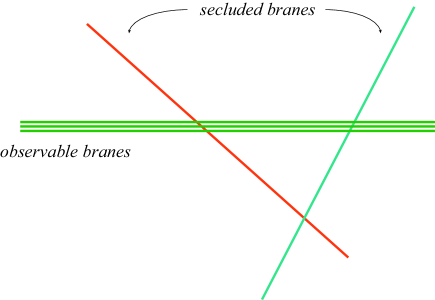
Figure 1: Our D-brane setup. The observable branes represent a supersymmetric version of the Standard Model. The secluded branes intersect in not supersymmetric angles with the observable sector breaking supersymmetry which is communicated to the observable sector via messenger strings aka strings stretched between the observable and secluded sector. Notice that this figure is just illustrative.

In order to perform our computations we consider toroidal compactifications of Type IIA with two D6-branes $a,~{}b$ in: $M_{4}\times T^{2}_{1}\times T^{2}_{2}\times T^{2}_{3}$. We assume non-SUSY configuration:

$$\theta^{ab}_{1}+\theta^{ab}_{2}+\theta^{ab}_{3}=\epsilon\approx 0$$ (1)

where $\theta_{ab}^{i}$ denotes the intersection angle of the two branes at the $i$th torus.

Different brane configurations preserve different amount of SUSY (figure 2):

• At ${\cal N}\approx 1$, branes intersect at all tori.

• At ${\cal N}\approx 2$ the branes are parallel in the first torus (aka $\theta^{1}_{ab}=0$) and intersect at non-sypersymmetric angles in the other two.

• At ${\cal N}\approx 4$ the branes are parallel in the first and second torus ($\theta^{1}_{ab}=\theta^{2}_{ab}=0$) and intersect with a small angle in the third torus $\theta^{3}_{ab}=\epsilon$.

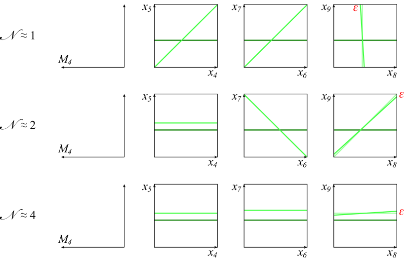
Figure 2: We consider D-branes intersecting at not supersymmetric angles. At ${\cal N}\approx 1$, branes intersect at all tori. At ${\cal N}\approx 2,~{}4$ there are parallel directions at one, two tori respectively. Notice that this figures are again illustrative. Thus, we omit the numerous wrapping of the distorted brane for simplicity. Another way to introduce the $\epsilon$ is to distort one of the tori (the third one in this case) by changing the modulus of the torus ($\tau_{3}$ of the third torus). This would not introduce multiple wrappings of the brane and is closer to what we have in mind in this work.

In this framework, we will calculate the 1-loop mass of the adjoint scalars.

3 Radiative masses for adjoint scalars

As we mention above we will focus on radiative corrections to masses of the adjoint scalars. There are two different kind of scalars and we will calculate their masses using different techniques:

• Adjoint scalars in non-parallel directions. We will evaluate the 1-loop mass of such fields by the standard conformal field theory method, by inserting vertex operators (VOs) at the boundaries of the corresponding surfaces. This method is the most general and could be performed in intersecting and parallel directions.

• Adjoint scalars in parallel directions. We will compute the partition function in the presence of brane-displacement and we will calculate the radiative corrections to the mass by taking derivatives of the displacements. This method can be performed only on parallel directions, but it is much easier.

3.1 Non-parallel directions by the standard amplitude method

As we have already mentioned, strings at the intersections feel the breaking of supersymmetry and they communicate it to the rest of the strings living on supersymmetric configurations. The scheme is similar to the field theory where non-supersymmetric messenger field generate mass split at 1-loop to other supersymmetric fields. In the string theory, the role of the messengers is played by the strings at the angles running in a loop (see figure 3).

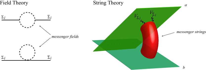
Figure 3: Equivalence of Field and String theory amplitudes. In field theory, supersymmetry is broken at tree level for the messengers running in the loops and it is communicated to $\Sigma_{i},~{}\bar{\Sigma}_{i}$ at 1-loop. In string theory, the role of the messenger fields is played by strings streached between the two branes.

3.1.1 The ${\cal N}\approx 1$ case

In such configuration D-branes intersect at all tori. The corresponding surface with boundaries is the annulus with the two VOs are inserted at the same boundary. The corresponding diagrams are:

$${\cal A}_{\Sigma_{3}\Sigma_{3}} = ig^{2}\int^{\infty}_{0}{dt}\int^{it/2}_{0}{dz_{1}}\int^{it/2}_{0}{dz_{2}}\int{d^{4}p\over(2\pi)^{4}}Tr[V(k;z_{1})V(k;z_{2})e^{L_{0}}]$$

$${\cal A}_{\Sigma_{3}\bar{\Sigma}_{3}} = ig^{2}\int^{\infty}_{0}{dt}\int^{it/2}_{0}{dz_{1}}\int^{it/2}_{0}{dz_{2}}\int{d^{4}p\over(2\pi)^{4}}Tr[V(k;z_{1})\bar{V}(k;z_{2})e^{L_{0}}]$$ (2)

where the vertex operators for the adjoint scalars are:

$$V_{\Sigma_{i}}(k,z) = 2g~{}(i\partial Z^{i}+\alpha^{\prime}(k\cdot\psi)\Psi^{i})e^{ik\cdot X(z)}$$

$$\bar{V}_{\bar{\Sigma}_{i}}(k,z) = 2g~{}(i\partial\bar{Z}^{i}-\alpha^{\prime}(k\cdot\psi)\bar{\Psi}^{i})e^{-ik\cdot X(z)}$$ (3)

and $k_{\mu}$ the momenta four-vectors.

The traces in (2) run over all word-sheet fields living on the annulus which is stretched between the D-branes $a$, $b$. By $p^{\mu}$ we denote the momenta running in the loop. The integrals run over all possible positions of the VOs $z_{1},~{}z_{2}\in[0,it/2)$ and the size of the annulus $t\in[0,\infty)$. Using translational invariance on the annulus we fix the second VO at zero: $z_{2}=0$.

The above amplitudes are zero on-shell if we enforce the conditions $k^{2}=0$. There is however a consistent off-shell extension which has given consistently the mass of bosons in other cases [31, 32, 35, 36, 37] and we adopt it here. We will impose these conditions only at the end of our calculations (after all integrations are performed). The amplitudes are:

$${\cal A}_{\Sigma_{3}\bar{\Sigma}_{3}}=-{g^{2}\over 16\pi^{4}\alpha^{\prime 3}}\int^{\infty}_{0}{dt\over t^{2}}\int^{it/2}_{0}{dz_{1}}~{}$$

$$~{}~{}~{}~{}~{}~{}~{}~{}~{}~{}~{}~{}~{}~{}~{}~{}~{}~{}~{}{\cal Z}_{{\cal M}_{4}}^{\cal B}Z_{ghost}^{\cal B}{\cal Z}_{{\cal T}_{1}^{2}}^{{\cal B},\theta^{1}}{\cal Z}_{{\cal T}_{2}^{2}}^{{\cal B},\theta^{2}}{\cal Z}_{{\cal T}_{3}^{2}}^{{\cal B},\theta^{3}}$$

$$~{}~{}~{}~{}~{}~{}~{}~{}~{}~{}~{}~{}~{}~{}~{}~{}~{}~{}~{}\times\sum_{ab}C[^{a}_{b}]{\cal Z}_{{\cal M}_{4}}^{\cal F}[^{a}_{b}]{\cal Z}_{ghost}^{\cal F}[^{a}_{b}]{\cal Z}_{{\cal T}_{1}^{2}}^{{\cal F},\theta^{1}}[^{a}_{b}]{\cal Z}_{{\cal T}_{2}^{2}}^{{\cal F},\theta^{2}}[^{a}_{b}]{\cal Z}_{{\cal T}_{3}^{2}}^{{\cal F},\theta^{3}}[^{a}_{b}]$$

$$~{}~{}~{}~{}~{}~{}~{}~{}~{}~{}~{}~{}~{}~{}~{}~{}~{}~{}~{}\times\Big{\langle}e^{ik\cdot X(z_{1})}e^{-ik\cdot X(0)}\Big{\rangle}$$

$$~{}~{}~{}~{}~{}~{}~{}~{}~{}~{}~{}~{}~{}~{}~{}~{}~{}~{}~{}\times\Big{(}\Big{\langle}\partial Z^{3}(z_{1})\partial\bar{Z}^{3}(0)\Big{\rangle}+\alpha^{\prime 2}k^{2}\Big{\langle}\psi(z_{1})\psi(0)\Big{\rangle}[^{a}_{b}]\Big{\langle}\Psi^{3}(z_{1})\bar{\Psi}^{3}(0)\Big{\rangle}[^{a}_{b}]\Big{)}$$ (4)

The correlation and the partition functions are given in the appendix. The sum over the spin structures is performed using the Riemann identity. After several steps we get an expression given only in terms of the well known theta-function $\vartheta_{1}(z,it/2)$:

$${\cal A}_{\Sigma_{3}\bar{\Sigma}_{3}} \approx -{2ig^{2}{{k^{2}}}\over 16\pi^{4}}I_{ab}\int^{\infty}_{0}{dt\over t^{2}}{\vartheta^{\prime}_{1}(0)^{2}\over\eta^{6}}{{\vartheta_{1}((\theta_{2}-\epsilon)it/2)}~{}{\vartheta_{1}((\theta_{3}-\epsilon)it/2)}\over\vartheta_{1}(\theta_{1}it/2)~{}\vartheta_{1}(\theta_{2}it/2)~{}\vartheta_{1}(\theta_{3}it/2)}$$

$$~{}~{}~{}~{}~{}~{}~{}~{}~{}~{}~{}~{}\times\int^{it/2}_{0}{dz_{1}}~{}e^{i{{k^{2}}}\langle X(z_{1})X(0)\rangle}e^{2\pi iz_{1}\theta_{1}}{\vartheta_{1}(z_{1}+\epsilon it/2)~{}\vartheta_{1}(z_{1}+(\theta_{1}-\epsilon)it/2)\over\vartheta_{1}(z_{1})^{2}}~{}~{}~{}~{}$$

where $I_{ab}$ is the intersection number of the two D-branes.

The last non-trivial step is to perform the integrals. Notice that the amplitude has an overall factor $k^{2}$. Thus, the only way to get a non-vanishing result on shell ($k^{2}=0$) is to find the integration limits that can provide a factor $1/k^{2}$. There are three different limits which we can generate a mass term for the above amplitude (figure 4):

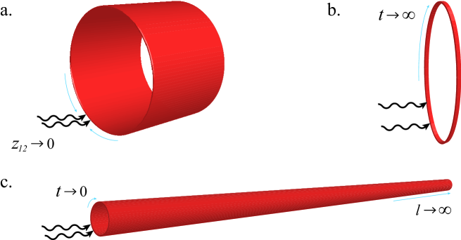
Figure 4: The three different limits which can generate a mass term for 1-loop open string amplitudes.

• World-sheet poles coming from the limit $z_{12}\to 0$. Single poles give us momentum poles via:

  $${\cal A}\sim k^{2}\int{dz_{1}}~{}\left({\vartheta_{1}(z_{1})\over\vartheta_{1}^{\prime}(0)}\right)^{-1-2\alpha^{\prime}k^{2}}\sim k^{2}\int{dz_{1}}~{}\left(z_{1}\right)^{-1-2\alpha^{\prime}k^{2}}\to{1\over 2\alpha^{\prime}}$$ (6)

  whereas double poles do not contribute as $k^{2}\to 0$ due to analytic continuation in $k^{2}$.

  In our case, there are poles both at $z_{1}=z_{2}=0$ and $z_{1}=it/2+z_{2}=it/2$, and they cancel.

• At the closed string UV limit (long strip limit $t\to\infty$). This is quite uncommon but might appear due to massless open strings running in the loop [39].

  In our case, there are no long strip contributions.

• At the closed string IR limit (long-tube limit $t\to 0$). This is due to the massless close-string exchange between the two annulus boundaries (notice the change of variables $l=1/t$) [35, 36].

  $${\cal A} \sim k^{2}\int{dl}~{}e^{-k^{2}\langle XX\rangle(z_{1})}~{}$$ (11)

  $$~{}~{}\sim~{}\left\{\begin{array}[]{llllll}\mbox{VOs on opposite boundaries}{}&~{}:~{}k^{2}\displaystyle\int_{a}^{\infty}dl~{}e^{-\pi\alpha^{\prime}k^{2}l}&~{}~{}\to{}&\displaystyle{1\over\pi\alpha^{\prime}}\\ \\ \mbox{VOs on the same boundary}{}&~{}:~{}k^{2}\displaystyle\int^{\infty}_{a}{dl}~{}(2\sin\pi x)^{-2\alpha^{\prime}k^{2}}&~{}~{}\to{}&\mbox{tadpoles}\end{array}\right.~{}~{}~{}$$

  Our case, fall in the second category and there are long tube contributions:

  $${\cal A}_{\Sigma_{3}\bar{\Sigma}_{3}}=-{ig^{2}\over 16\pi^{3}\alpha^{\prime}}\Big{(}{{\cal V}^{1}_{a}{\cal V}^{1}_{b}\over T^{1}_{2}}{{\cal V}^{2}_{a}{\cal V}^{2}_{b}\over T^{2}_{2}}{{\cal V}^{3}_{a}{\cal V}^{3}_{b}\over T^{3}_{2}}\Big{)}\Big{(}-1+\cos^{2}[\pi\theta_{1}]+\cos^{2}[\pi\theta_{2}]-\cos^{2}[\pi\theta_{3}]\Big{)}~{}~{}~{}~{}$$

  where ${\cal V}_{a(b)}^{i}$ the world-volume of the D-brane in the $a~{}(b)$ directions of the $i$th torus. Also $T^{i}_{2}$ is the Kähler modulus of the $i$th torus.

  Notice however, that this tadpole does not depend on the supersymmetry breaking parameter $\epsilon$. This result was expected also in supersymmetric frameworks and it is cancelled in all consistent models (without R-R and NS-NS tadpoles) by a similar tadpole which comes from the Möbius strip amplitude [31, 32].

We can therefore conclude that there is no contribution to the masses of the adjoint scalars from ${\cal N}\approx 1$ sectors.

3.2 Parallel directions by brane displacement method.

Next, we will evaluate the radiative corrections for the masses of adjoint scalars in parallel directions. Such scalars appear only in the ${\cal N}\approx 2,4$ cases. We could perform a similar calculation to the above, but for sake of simplicity we will use a different approach: We will evaluate the 1-loop partition function at the presence of some displacements of the branes in the parallel directions (fig 5). This will give us the potential for these dicplacements and we can easilly evaluate the induced 1-loop mass for these fields by taking the second derivative.

The 1-loop partition function is:

$${\cal Z}(it/2) ~{}~{}\sim~{}~{} {\cal Z}_{{\cal M}_{4}}^{\cal B}{\cal Z}_{ghost}^{\cal B}{\cal Z}_{{\cal T}_{1}^{2}}^{\cal B}{\cal Z}_{{\cal T}_{2}^{2}}^{\cal B}{\cal Z}_{{\cal T}_{3}^{2}}^{\cal B}~{}\times~{}{\cal Z}_{{\cal M}_{4}}^{\cal F}{\cal Z}_{ghost}^{\cal F}{\cal Z}_{{\cal T}_{1}^{2}}^{\cal F}{\cal Z}_{{\cal T}_{2}^{2}}^{\cal F}{\cal Z}_{{\cal T}_{3}^{2}}^{\cal F}$$ (12)

A displacement of the branes by $\Sigma_{i}$ in parallel directions would only affect the bosonic partition function of this torus.

$${\cal Z}_{{\cal T}_{i}^{2}}^{{\cal B},||}(\Sigma^{i}_{1},l^{i}+\Sigma^{i}_{2})={1\over\eta^{2}}\sum_{m_{i},n_{i}}e^{2\pi i\tau\big{(}\big{(}\Sigma^{i}_{1}+{m_{i}\over R_{1,i}}\big{)}^{2}+\big{(}l^{i}+\Sigma^{i}_{2}+{n_{i}R_{2,i}}\big{)}^{2}\big{)}}$$ (13)

Next, we will consider separately the ${\cal N}\approx 2,~{}4$ cases.

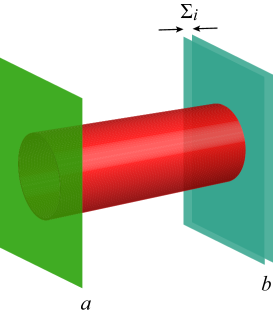
Figure 5: Displacing the branes by $\Sigma_{i}$ in parallel directions.

3.2.1 The ${\cal N}\approx 2$ case

The total 1-loop partition function is given by

$${\cal Z}(it/2) \sim {\cal Z}_{{\cal M}_{4}}^{\cal B}{\cal Z}_{ghost}^{\cal B}{\cal Z}_{{\cal T}_{1}^{2}}^{\cal B,||}(l){\cal Z}_{{\cal T}_{2}^{2}}^{\cal B,\angle}(\theta_{2}){\cal Z}_{{\cal T}_{3}^{2}}^{\cal B,\angle}(\theta_{3})$$ (14)

$${\cal Z}_{{\cal M}_{4}}^{\cal F}{\cal Z}_{ghost}^{\cal F}{\cal Z}_{{\cal T}_{1}^{2}}^{\cal F,||}(l){\cal Z}_{{\cal T}_{2}^{2}}^{\cal F,\angle}(\theta_{2}){\cal Z}_{{\cal T}_{3}^{2}}^{\cal F,\angle}(\theta_{3})$$

where we insert a displacement in the first torus. The potential for the ${\cal N}\approx 2$ case is:

$${\cal V}(\Sigma^{1}_{1},\Sigma^{1}_{2}) = {i\over 32\pi^{4}\alpha^{\prime}}\int^{\infty}_{0}{dt\over t^{3}}{\cal Z}_{{\cal M}_{4}}^{\cal B}{\cal Z}_{ghost}^{\cal B}{\cal Z}_{{\cal T}_{1}^{2}}^{{\cal B},||}(\Sigma^{1}_{1},l^{1}+\Sigma^{1}_{2}){\cal Z}_{{\cal T}_{2}^{2}}^{{\cal B},\theta^{2}}{\cal Z}_{{\cal T}_{3}^{2}}^{{\cal B},\theta^{3}}$$ (15)

$$~{}~{}~{}~{}~{}~{}~{}~{}~{}~{}~{}~{}~{}~{}~{}~{}~{}\times\sum_{ab}C[^{a}_{b}]{\cal Z}_{{\cal M}_{4}}^{\cal F}[^{a}_{b}]{\cal Z}_{ghost}^{\cal F}[^{a}_{b}]{\cal Z}_{{\cal T}_{1}^{2}}^{{\cal F},||}[^{a}_{b}]{\cal Z}_{{\cal T}_{2}^{2}}^{{\cal F},\theta^{2}}[^{a}_{b}]{\cal Z}_{{\cal T}_{3}^{2}}^{{\cal F},\theta^{3}}[^{a}_{b}]$$

By taking derivatives on $\Sigma_{i}$’s and letting afterwards $\Sigma_{i}\to 0$ we get the tadpoles:

$${\cal V}^{(0,1)}~{}\sim~{}-32\pi^{2}\varepsilon^{2}\displaystyle\sum_{m,n}\frac{l+nR_{2,1}}{(mR_{1,1})^{2}+\left(l+nR_{2,1}\right)^{2}}~{}~{}\neq~{}~{}0$$ (16)

$${\cal V}^{(1,0)}~{}\sim~{}-32\pi^{2}\varepsilon^{2}\displaystyle\sum_{m,n}\frac{mR_{1,1}}{(mR_{1,1})^{2}+\left(l+nR_{2,1}\right)^{2}}~{}~{}\rightarrow~{}~{}0$$ (17)

where by ${\cal V}^{(i,j)}$ we denote the $i$th, $j$th derivatives of the potential over $\Sigma_{1},~{}\Sigma_{2}$ respectively.

Notice that the ${\cal V}^{(1,0)}$ is an odd function on $m$ and consequently vanishes running over all integers from $-\infty$ to $\infty$. The tadpole from ${\cal V}^{(0,1)}$ can also be eliminated if we add another secluded brane at distance $-l$.

In order to get the mass-matrix for the adjoint fields we evaluate second derivatives on $\Sigma_{i}$’s:

$${\cal V}^{(2,0)}~{}\sim~{}~{}~{}32\pi^{2}\varepsilon^{2}\displaystyle\sum_{m,n}\frac{(mR_{1,1})^{2}+\left(l+nR_{2,1}\right)^{2}}{\left[(mR_{1,1})^{2}+\left(l+nR_{2,1}\right)^{2}\right]^{2}}~{}~{}\leq~{}~{}0$$ (18)

$${\cal V}^{(0,2)}~{}\sim-32\pi^{2}\varepsilon^{2}\displaystyle\sum_{m,n}\frac{(mR_{1,1})^{2}-\left(l+nR_{2,1}\right)^{2}}{\left[(mR_{1,1})^{2}+\left(l+nR_{2,1}\right)^{2}\right]^{2}}~{}~{}\geq~{}~{}0$$ (19)

$${\cal V}^{(1,1)}~{}\sim~{}~{}~{}64\pi^{2}\varepsilon^{2}\displaystyle\sum_{m,n}\frac{(mR_{1,1})\left(l+nR_{2,1}\right)}{\left[(mR_{1,1})^{2}+\left(l+nR_{2,1}\right)^{2}\right]^{2}}~{}\rightarrow~{}~{}0$$ (20)

However, the mass-matrix for the adjoint scalars is traceless (since ${\cal V}^{(2,0)}=-{\cal V}^{(0,2)}$) denoting the presence of two opposite-sign entries. This fact leads to tachyonic states. Their presence cannot be annihilated with the addition of an image brane.

3.2.2 The ${\cal N}\approx 4$ case

In this case the partition function is:

$${\cal V}(it/2) \sim {\cal Z}_{{\cal M}_{4}}^{\cal B}{\cal Z}_{ghost}^{\cal B}{\cal Z}_{{\cal T}_{1}^{2}}^{\cal B,||}(l_{1}){\cal Z}_{{\cal T}_{2}^{2}}^{\cal B,||}(l_{2}){\cal Z}_{{\cal T}_{3}^{2}}^{\cal B,\angle}(\epsilon)$$ (21)

$${\cal Z}_{{\cal M}_{4}}^{\cal F}{\cal Z}_{ghost}^{\cal F}{\cal Z}_{{\cal T}_{1}^{2}}^{\cal F,||}(l_{1}){\cal Z}_{{\cal T}_{2}^{2}}^{\cal F,||}(l_{2}){\cal Z}_{{\cal T}_{3}^{2}}^{\cal F,\angle}(\epsilon)$$

We insert a displacement in both tori ${\cal T}^{2}_{1},~{}{\cal T}^{2}_{2}$. The potential for the ${\cal N}\approx 4$ case reads:

$${\cal V}(\Sigma_{1,i},~{}\Sigma_{2,i})\sim-4\pi^{2}\varepsilon^{3}~{}\bigg{(}\sum_{i=1,2}\left(({\Sigma_{1,i}+\tilde{n}_{i}R_{1,i}})^{2}+(\Sigma_{2,i}+l_{i}+{n_{i}R_{2,i}})^{2}\right)\bigg{)}^{-1}$$ (22)

Taking derivatives on $\Sigma_{1,1},~{}\Sigma_{2,1},~{}\Sigma_{2,1},~{}\Sigma_{2,2}$ and setting all $\Sigma_{i,j}\to 0$ we get the tadpoles:

$${\cal V}^{(1,0,0,0)} ~{}\sim~{} {8\pi^{2}|\varepsilon|^{3}}~{}\sum_{\tilde{n},n}{\tilde{n}_{1}R_{1,1}\over(\sum_{i}\left(({\tilde{n}_{i}R_{1,i}})^{2}+(l_{i}+{n_{i}R_{2,i}})^{2}\right))^{2}}~{}~{}\to~{}~{}0$$ (23)

$${\cal V}^{(0,1,0,0)} ~{}\sim~{} {8\pi^{2}|\varepsilon|^{3}}~{}\sum_{\tilde{n},n}{l_{1}+n_{2}R_{2,1}\over(\sum_{i}\left(({\tilde{n}_{i}R_{1,i}})^{2}+(l_{i}+{n_{i}R_{2,i}})^{2}\right))^{2}}~{}~{}\neq~{}~{}~{}0$$ (24)

$${\cal V}^{(0,0,1,0)} ~{}\sim~{} {8\pi^{2}|\varepsilon|^{3}}~{}\sum_{\tilde{n},n}{\tilde{n}_{2}R_{1,2}\over(\sum_{i}\left(({\tilde{n}_{i}R_{1,i}})^{2}+(l_{i}+{n_{i}R_{2,i}})^{2}\right))^{2}}~{}~{}\to~{}~{}0$$ (25)

$${\cal V}^{(0,0,0,1)} ~{}\sim~{} {8\pi^{2}|\varepsilon|^{3}}~{}\sum_{\tilde{n},n}{l_{1}+n_{2}R_{2,2}\over(\sum_{i}\left(({\tilde{n}_{i}R_{1,i}})^{2}+(l_{i}+{n_{i}R_{2,i}})^{2}\right))^{2}}~{}~{}\neq~{}~{}~{}0$$ (26)

The non-vanishing tadpoles can be cancelled by properly choosing image branes (since the tadpoles are odd on the distances $l_{i}$ we can put image branes on distance $-l_{i}$).

In order to get the mass-matrix we evaluate:

$$\begin{array}[]{rrrrrrr}{\cal V}^{(2,0,0,0)}&~{}\sim{}&~{}16i\pi^{2}|\varepsilon|^{3}\displaystyle\sum_{\tilde{n},n}{-4(\tilde{n}_{1}R_{1,1})^{2}+S[\tilde{n},n]\over S[\tilde{n},n]^{3}{}{}{}}&~{}~{}~{}\neq~{}~{}0\\ {\cal V}^{(1,1,0,0)}&~{}\sim{}&~{}16i\pi^{2}|\varepsilon|^{3}\displaystyle\sum_{\tilde{n},n}{4(\tilde{n}_{1}R_{1,1})(l_{1}+n_{1}R_{2,1})\over S[\tilde{n},n]^{3}}&\to~{}~{}0\\ {\cal V}^{(1,0,1,0)}&~{}\sim{}&~{}16i\pi^{2}|\varepsilon|^{3}\displaystyle\sum_{\tilde{n},n}{4(\tilde{n}_{1}R_{1,1})(\tilde{n}_{2}R_{1,2})\over S[\tilde{n},n]^{3}}&\to~{}~{}0\\ {\cal V}^{(1,0,0,1)}&~{}\sim{}&~{}16i\pi^{2}|\varepsilon|^{3}\displaystyle\sum_{\tilde{n},n}{4(\tilde{n}_{1}R_{1,1})(l_{2}+n_{2}R_{2,2})\over S[\tilde{n},n]^{3}}&\to~{}~{}0\\ {\cal V}^{(0,2,0,0)}&~{}\sim{}&~{}16i\pi^{2}|\varepsilon|^{3}\displaystyle\sum_{\tilde{n},n}{-4(l_{1}+n_{1}R_{2,1})^{2}+S[\tilde{n},n]\over S[\tilde{n},n]^{3}}&\neq~{}~{}0\\ {\cal V}^{(0,1,1,0)}&~{}\sim{}&~{}16i\pi^{2}|\varepsilon|^{3}\displaystyle\sum_{\tilde{n},n}{4(l_{1}+n_{1}R_{2,1})(\tilde{n}_{2}R_{1,2})\over S[\tilde{n},n]^{3}}&\to~{}~{}0\\ {\cal V}^{(0,1,0,1)}&~{}\sim{}&~{}16i\pi^{2}|\varepsilon|^{3}\sum_{\tilde{n},n}{4(l_{1}+\tilde{n}_{1}R_{1,1})(l_{2}+n_{2}R_{2,2})\over S[\tilde{n},n]^{3}}&\neq~{}~{}0\\ {\cal V}^{(0,0,2,0)}&~{}\sim{}&~{}16i\pi^{2}|\varepsilon|^{3}\displaystyle\sum_{\tilde{n},n}{-4(\tilde{n}_{2}R_{1,2})^{2}+S[\tilde{n},n]\over S[\tilde{n},n]^{3}}&\neq~{}~{}0\\ {\cal V}^{(0,0,1,1)}&~{}\sim{}&~{}16i\pi^{2}|\varepsilon|^{3}\displaystyle\sum_{\tilde{n},n}{4(\tilde{n}_{2}R_{1,2})(l_{2}+n_{2}R_{2,2})\over S[\tilde{n},n]^{3}}&\to~{}~{}0\\ {\cal V}^{(0,0,0,2)}&~{}\sim{}&~{}16i\pi^{2}|\varepsilon|^{3}\displaystyle\sum_{\tilde{n},n}{-4(l_{2}+n_{2}R_{2,2})^{2}+S[\tilde{n},n]\over S[\tilde{n},n]^{3}}&\neq~{}~{}0\end{array}$$ (37)

where $S[\tilde{n},n]=(\tilde{n}_{1}R_{1,1})^{2}+(l_{1}+n_{1}R_{2,1})^{2}+(\tilde{n}_{2}R_{1,2})^{2}+(l_{2}+n_{2}R_{2,2})^{2}$. Here again, all odd functions on the winding numbers vanish. Schematically, the mass matrix is given by:

$${\cal M}^{2}_{N\approx 4}~{}\sim{|\epsilon|^{3}g^{2}|I_{ab}|\over 32\pi^{2}\alpha^{\prime}}{\tiny\left(~{}\begin{array}[]{cccc}A_{1,2}^{2}+A_{2,1}^{2}+A_{2,2}^{2}-3A_{1,1}^{2}&0&0&0\\ 0&A_{1,1}^{2}+A_{2,1}^{2}+A_{2,2}^{2}-3A_{1,2}^{2}&0&-A_{1,2}A_{2,2}\\ 0&0&A_{1,1}^{2}+A_{1,2}^{2}+A_{2,2}^{2}-3A_{2,1}^{2}&0\\ 0&-A_{1,2}A_{2,2}&0&A_{1,1}^{2}+A_{1,2}^{2}+A_{2,1}^{2}-3A_{2,2}^{2}\end{array}~{}\right)}~{}~{}~{}~{}~{}~{}~{}~{}~{}$$ (42)

and again it is traceless. Therefore, there is at least one tachyonic state.

4 Conclusions

We considered breaking of supersymmetry in intersecting D-brane configurations by slight deviation of the angles from their supersymmetric values. We computed the masses generated by radiative corrections for the adjoint scalars on the brane world-volumes.

In the open string channel, the string two-point function receives contributions only from the infrared (${\cal N}\approx 2,~{}4$) and the ultraviolet limits (${\cal N}\approx 1$). The latter is due to tree-level closed string uncanceled tadpoles which will be eliminated in all consistent models (without R-R, NS-NS tedpoles).

On the other hand, the infrared region (${\cal N}\approx 2,~{}4$) reproduces the one-loop mediation of supersymmetry breaking in the effective gauge theory, via messengers and their Kaluza-Klein excitations.

APPENDIX

Appendix A Theta functions and modular invariance

In this short appendix, we establish our conventions for the modular theta functions and list a few useful properties. The theta functions are defined by:

$$\vartheta[^{a}_{b}](z|\tau)=\sum_{n=-\infty}^{\infty}e^{\pi i(n+a)^{2}\tau+2\pi i(n+a)(z+b)}$$ (A.43)

where $\tau$ is the (complex) modular parameter of the torus, not to be confused with the world-sheet coordinate used in the text. On the cylinder, this parameter is purely imaginary and in the main text we use the definition $\tau=it/2$. Alternatively, the theta functions can be defined as an infinite product:

$$\vartheta[^{a}_{b}](z|\tau)=e^{2\pi ia(b+z)}q^{\frac{1}{2}a^{2}}\prod_{n\geq 1}(1+q^{n+a-\frac{1}{2}}e^{2\pi i(b+z)})(1+q^{n-a-\frac{1}{2}}e^{-2\pi i(b+z)})(1-q^{n})$$ (A.44)

where $q=e^{2\pi i\tau}$. Defining $\vartheta_{1}(z)\equiv\vartheta[^{1/2}_{1/2}](z|\tau)~{},~{}~{}\vartheta_{2}(z)\equiv\vartheta[^{1/2}_{~{}0}](z|\tau)~{},~{}~{}\vartheta_{3}(z)\equiv\vartheta[^{0}_{0}](z|\tau)~{},~{}~{}\vartheta_{4}(z)\equiv\vartheta[^{~{}0}_{1/2}](z|\tau)$. In particular $\vartheta_{1}(z)=z\vartheta^{\prime}_{1}(0)+\cdots\$ a fact that was used repeatedly in the main text.

The Dedekind eta function is $\eta(\tau)=q^{\frac{1}{24}}\prod_{n\geq 1}(1-q^{n})$ and it is related to the function $\vartheta_{1}(z)$ by the simple identity

$$\vartheta^{\prime}_{1}(0)=-2\pi\eta(\tau)^{3}$$ (A.45)

Finally, the theta functions satisfy the following Riemann identity:

$$\sum_{a,b}C_{a,b}\vartheta[^{a}_{b}](z_{1})\vartheta[^{a}_{b}](z_{2})\vartheta[^{a}_{b}](z_{3})\vartheta[^{a}_{b}](z_{4})=2\vartheta_{1}(z^{\prime}_{1})\vartheta_{1}(z^{\prime}_{2})\vartheta_{1}(z^{\prime}_{3})\vartheta_{1}(z^{\prime}_{4})$$ (A.46)

with $z^{\prime}_{1}=\frac{1}{2}(z_{1}+z_{2}+z_{3}+z_{4}),~{}z^{\prime}_{2}=\frac{1}{2}(z_{1}+z_{2}-z_{3}-z_{4}),~{}z^{\prime}_{3}=\frac{1}{2}(z_{1}-z_{2}+z_{3}-z_{4}),~{}z^{\prime}_{4}=\frac{1}{2}(z_{1}-z_{2}-z_{3}+z_{4}).$

Appendix B Partition functions

The partition functions of the bosonic and fermionic modes are:

$$\begin{array}[]{lllllll}{\bf Bosonic}&&{\bf Fermionic}\\ \mathcal{Z}_{{\cal M}_{4}}^{\cal B}={1\over\eta^{4}}&{}{}{}{}{}{}{}{}{}{}{}{}{}{}{}&\mathcal{Z}_{{\cal M}_{4}}^{\cal F}={\vartheta[_{a}^{b}]^{2}\over\eta^{2}}\\ \mathcal{Z}_{ghost}^{\cal B}={\eta^{2}}&&\mathcal{Z}_{ghost}^{\cal F}={\eta\over\vartheta[_{a}^{b}]}\\ \mathcal{Z}_{{\cal T}_{i}^{2}}^{{\cal B},||}(l_{i})={\Lambda_{m_{i},n_{i}}(l_{i})\over\eta^{2}}={1\over\eta^{2}}\sum_{m_{i},n_{i}}e^{2\pi i\tau\big{[}({m_{i}\over R_{1,i}})^{2}+(l_{i}+{n_{i}R_{2,i}})^{2}\big{]}}&&\mathcal{Z}_{{\cal T}_{i}^{2}}^{{\cal F},||}={\vartheta[_{a}^{b}]\over\eta}\\ \mathcal{Z}_{{\cal T}_{i}^{2}}^{{\cal B},\angle}(\alpha)={\eta\over\vartheta[_{~{}~{}1/2}^{1/2+\alpha}]}&&\mathcal{Z}_{{\cal T}_{i}^{2}}^{{\cal F},\angle}(\alpha)={\vartheta[_{~{}a}^{b+\alpha}]\over\eta{}{}{}{}{}{}{}{}}\end{array}~{}~{}~{}~{}$$ (B.52)

where we have omitted the argument of the theta-function which are evaluated in $\tau=it/2$, $\nu=0$. In addition we have introduced twisted theta function and we have indicated with $ab$ the spin structures.

We also use the Poisson resummation formula:

$$\sum_{n\in Z}e^{-\pi an^{2}+\pi bn}={1\over\sqrt{a}}\sum_{n\in Z}e^{-{\pi\over a}\left(n+i{b\over 2}\right)^{2}}$$ (B.53)

in order to T-dualize the longitudinal directions of the brane $X_{i}$.

Appendix C Correlation functions

The untwisted correlators on the torus are:

$$\langle X(z_{1})X(z_{2})\rangle_{\cal T}=-{1\over 4}\log\left|{\vartheta_{1}(z_{12}|\tau)\over\vartheta^{\prime}_{1}(0|\tau)}\right|^{2}+{\pi\Im^{2}(z_{12})\over 2\tau_{2}}$$ (C.54)

$$\langle\partial Z(z_{1})Z(z_{2})\rangle_{\cal T}=-{1\over 4}{\vartheta_{1}^{\prime}(z_{12}|\tau)\over\vartheta_{1}(z_{12}|\tau)}+{\pi\over 2\tau_{2}}\partial_{z_{12}}{\Im^{2}(z_{12})}$$ (C.55)

$$\langle\psi(z_{1})\psi(z_{2})\rangle_{{\cal T}}={i\over 2}{\vartheta[_{a}^{b}](z_{12}|\tau)\vartheta^{\prime}_{1}(0|\tau)\over\vartheta_{1}(z_{12}|\tau)\vartheta[_{a}^{b}](0|\tau)}$$ (C.56)

The twisted correlators:

$$\langle Z(z_{1})\partial\bar{Z}(z_{2})\rangle_{{\cal T},\alpha}=-\frac{1}{2}{\vartheta_{1}^{\alpha}(z_{12})\vartheta_{1}^{\prime}(0)\over\vartheta_{1}^{\alpha}(0)\vartheta_{1}(z_{12})}$$ (C.57)

$$\langle\psi(z_{1})\psi(z_{2})\rangle_{{\cal T},\alpha}={i\over 2}{\vartheta[_{a}^{b}]^{\alpha}(z_{12}|\tau)\vartheta^{\prime}_{1}(0|\tau)\over\vartheta_{1}(z_{12}|\tau)\vartheta^{\alpha}[_{a}^{b}](0|\tau)}$$ (C.58)

Notice that all correlation functions are periodic on the torus: $x_{12}\to x_{12}+1$ and $x_{12}\to x_{12}+\tau$.

In order to define the correlators on the annulus and Möbius strip we use the involution: $I_{\cal A}=I_{\cal M}=1-\bar{z}$:

$$\langle X(z_{1})X(z_{2})\rangle_{\sigma} = {1\over 2}\Big{(}\langle X(z_{1})X(z_{2})\rangle_{\cal T}+\langle X(z_{1})X(I_{\sigma}(z_{2}))\rangle_{\cal T}$$ (C.59)

$$~{}~{}~{}+\langle X(I_{\sigma}(z_{1}))X(z_{2})\rangle_{\cal T}+\langle X(I_{\sigma}(z_{1}))X(I_{\sigma}(z_{2}))\rangle_{\cal T}\Big{)}$$

In our case, $z_{1}=iv,~{}z_{2}=0,~{}\tau=it/2$ that gives $\langle X(z_{1})X(z_{2})\rangle_{\sigma}=2\langle X(z_{1})X(z_{2})\rangle_{\cal T}$ and the untwisted correlators:

$$\langle X(z_{12})X(0)\rangle_{\cal A}=-\log{\vartheta_{1}(z_{12}|\tau)\over\vartheta^{\prime}_{1}(0|\tau)}+{2\pi z_{12}^{2}\over t}-{\pi i\over 2}$$ (C.60)

$$\langle\partial X(z_{12})X(0)\rangle_{\cal A}=-{\vartheta_{1}^{\prime}(z_{12}|\tau)\over\vartheta_{1}(z_{12}|\tau)}+{4\pi z_{12}\over t}$$ (C.61)

$$\langle\psi(z_{12})\psi(0)\rangle_{{\cal A}}={i}{\vartheta_{ab}(z_{12}|\tau)\vartheta^{\prime}_{1}(0|\tau)\over\vartheta_{1}(z_{12}|\tau)\vartheta_{ab}(0|\tau)}$$ (C.62)

The twisted correlators:

$$\langle Z(z_{1})\partial\bar{Z}(z_{2})\rangle_{{\cal A},\alpha}=-{\vartheta_{1}^{\alpha}(z_{12})\vartheta_{1}^{\prime}(0)\over\vartheta_{1}^{\alpha}(0)\vartheta_{1}(z_{12})}$$ (C.63)

$$\langle\psi(z_{1})\psi(z_{2})\rangle_{{\cal A},\alpha}={i}{\vartheta_{ab}^{\alpha}(z_{12}|\tau)\vartheta^{\prime}_{1}(0|\tau)\over\vartheta_{1}(z_{12}|\tau)\vartheta^{\alpha}_{ab}(0|\tau)}$$ (C.64)

References

• [1] R. Blumenhagen, M. Cvetic, P. Langacker and G. Shiu, Ann. Rev. Nucl. Part. Sci.  55 (2005) 71 [hep-th/0502005].
• [2] R. Blumenhagen, B. Kors, D. Lust and S. Stieberger, Phys. Rept.  445 (2007) 1 [hep-th/0610327].
• [3] F. Marchesano, Fortsch. Phys.  55 (2007) 491 [hep-th/0702094 [HEP-TH]].
• [4] M. Bianchi, arXiv:0909.1799 [hep-th].
• [5] E. Dudas and J. Mourad, Nucl. Phys. B 575, 3 (2000) [hep-th/9911019].
• [6] E. Accomando, I. Antoniadis, and K. Benakli, Looking for TeV scale strings and extra dimensions, Nucl.Phys. B579 (2000) 3–16, [hep-ph/9912287].
• [7] S. Cullen, M. Perelstein, and M. E. Peskin, TeV strings and collider probes of large extra dimensions, Phys.Rev. D62 (2000) 055012, [hep-ph/0001166].
• [8] E. Kiritsis and P. Anastasopoulos, The Anomalous magnetic moment of the muon in the D-brane realization of the standard model, JHEP 0205 (2002) 054, [hep-ph/0201295].
• [9] P. Burikham, T. Figy, and T. Han, TeV-scale string resonances at hadron colliders, Phys.Rev. D71 (2005) 016005, [hep-ph/0411094].
• [10] D. Chialva, R. Iengo, and J. G. Russo, Cross sections for production of closed superstrings at high energy colliders in brane world models, Phys.Rev. D71 (2005) 106009, [hep-ph/0503125].
• [11] M. Bianchi and A. V. Santini, String predictions for near future colliders from one-loop scattering amplitudes around D-brane worlds, JHEP 0612 (2006) 010, [hep-th/0607224].
• [12] L. A. Anchordoqui, H. Goldberg, S. Nawata, and T. R. Taylor, Jet signals for low mass strings at the LHC, Phys.Rev.Lett. 100 (2008) 171603, [arXiv:0712.0386].
• [13] P. Anastasopoulos, F. Fucito, A. Lionetto, G. Pradisi, A. Racioppi, and Ya. Stanev, Minimal Anomalous U(1)-prime Extension of the MSSM, Phys.Rev. D78 (2008) 085014, [arXiv:0804.1156].
• [14] L. A. Anchordoqui, H. Goldberg, S. Nawata, and T. R. Taylor, Direct photons as probes of low mass strings at the CERN LHC, Phys.Rev. D78 (2008) 016005, [arXiv:0804.2013].
• [15] Z. Dong, T. Han, M.-x. Huang, and G. Shiu, Top Quarks as a Window to String Resonances, JHEP 1009 (2010) 048, [arXiv:1004.5441].
• [16] D. Lust, S. Stieberger and T. R. Taylor, Nucl. Phys. B 808 (2009) 1 [arXiv:0807.3333 [hep-th]].
• [17] D. Lust, O. Schlotterer, S. Stieberger and T. R. Taylor, Nucl. Phys. B 828, 139 (2010) [arXiv:0908.0409 [hep-th]].
• [18] L. A. Anchordoqui, H. Goldberg, D. Lust, S. Nawata, S. Stieberger and T. R. Taylor, Nucl. Phys. B 821 (2009) 181 [arXiv:0904.3547 [hep-ph]].
• [19] W. -Z. Feng, D. Lust, O. Schlotterer, S. Stieberger and T. R. Taylor, Nucl. Phys. B 843 (2011) 570 [arXiv:1007.5254 [hep-th]].
• [20] P. Anastasopoulos, M. Bianchi and R. Richter, arXiv:1110.5424 [hep-th].
• [21] C. Bachas, “A Way to break supersymmetry,” arXiv:hep-th/9503030.
• [22] C. Angelantonj, I. Antoniadis, E. Dudas and A. Sagnotti, “Type I strings on magnetized orbifolds and brane transmutation,” Phys. Lett.  B 489, 223 (2000) [arXiv:hep-th/0007090].
• [23] M. Berkooz, M. R. Douglas and R. G. Leigh, “Branes intersecting at angles,” Nucl. Phys.  B 480, 265 (1996) [arXiv:hep-th/9606139].
• [24] R. Blumenhagen, L. Goerlich, B. Kors and D. Lust, “Noncommutative compactifications of type I strings on tori with magnetic JHEP 0010, 006 (2000) [arXiv:hep-th/0007024].
• [25] I. Antoniadis, K. Benakli, A. Delgado, M. Quiros and M. Tuckmantel, “Split extended supersymmetry from intersecting branes”, Nucl. Phys.  B 744 (2006) 156 [arXiv:hep-th/0601003].
• [26] I. Antoniadis, A. Delgado, K. Benakli, M. Quiros and M. Tuckmantel, “Splitting extended supersymmetry,” Phys. Lett.  B 634, 302 (2006) [arXiv:hep-ph/0507192].
• [27] I. Antoniadis, E. Gava, K. S. Narain and T. R. Taylor, “Duality in superstring compactifications with magnetic field backgrounds,” Nucl. Phys.  B 511, 611 (1998) [arXiv:hep-th/9708075].
S. Kachru and J. McGreevy, “Supersymmetric three cycles and supersymmetry breaking,” Phys. Rev.  D 61, 026001 (2000) [arXiv:hep-th/9908135].
M. Mihailescu, I. Y. Park and T. A. Tran, “D-branes as solitons of an N=1, D = 10 noncommutative gauge theory,” Phys. Rev.  D 64, 046006 (2001) [arXiv:hep-th/0011079].
E. Witten, “BPS Bound states of D0 - D6 and D0 - D8 systems in a B field,” JHEP 0204, 012 (2002) [arXiv:hep-th/0012054].
D. Cremades, L. E. Ibanez and F. Marchesano, “SUSY quivers, intersecting branes and the modest hierarchy problem,” JHEP 0207, 009 (2002) [arXiv:hep-th/0201205].
I. Antoniadis, K. S. Narain and T. R. Taylor, “Open string topological amplitudes and gaugino masses,” Nucl. Phys.  B 729, 235 (2005) [arXiv:hep-th/0507244].
L. E. Ibanez, F. Marchesano and R. Rabadan, “Getting just the standard model at intersecting branes,” JHEP 0111, 002 (2001) [arXiv:hep-th/0105155].
• [28] P. Anastasopoulos, I. Antoniadis, K. Benakli, M. D. Goodsell and A. Vichi, “One-loop adjoint masses for non-supersymmetric intersecting branes,” JHEP 1108 (2011) 120 [arXiv:1105.0591 [hep-th]].
• [29] M. Gomez-Reino and I. Zavala, “Recombination of intersecting D-branes and cosmological inflation,” JHEP 0209 (2002) 020 [arXiv:hep-th/0207278].
• [30] A. Hebecker, S. C. Kraus, D. Lust, S. Steinfurt and T. Weigand, “Fluxbrane Inflation,” arXiv:1104.5016 [hep-th].
• [31] E. Poppitz, “On the one loop Fayet-Iliopoulos term in chiral four-dimensional type I orbifolds,” Nucl. Phys. B 542 (1999) 31 [arXiv:hep-th/9810010].
• [32] P. Bain and M. Berg, “Effective action of matter fields in four-dimensional string orientifolds,” JHEP 0004 (2000) 013 [arXiv:hep-th/0003185].
• [33] K. Benakli and M. D. Goodsell, “Two-Point Functions of Chiral Fields at One Loop in Type II,” Nucl. Phys.  B 805 (2008) 72 [arXiv:0805.1874 [hep-th]].
• [34] J. P. Conlon, M. Goodsell and E. Palti, “Anomaly Mediation in Superstring Theory,” arXiv:1008.4361 [hep-th].
• [35] I. Antoniadis, E. Kiritsis and J. Rizos, “Anomalous U(1)s in type I superstring vacua,” Nucl. Phys.  B 637 (2002) 92 [arXiv:hep-th/0204153].
• [36] P. Anastasopoulos, “4D anomalous U(1)’s, their masses and their relation to 6D anomalies,” JHEP 0308 (2003) 005 [arxiv:hep-th/0306042]
P. Anastasopoulos, “Anomalous U(1)s masses in non-supersymmetric open string vacua,” Phys. Lett. B 588 (2004) 119 [arxiv:hep-th/0402105].
P. Anastasopoulos, “Thesis: Orientifolds, anomalies and the standard model,” [hep-th/0503055].
• [37] M. Berg, M. Haack and J. U. Kang, arXiv:1112.5156 [hep-th].
• [38] W. Fischler, L. Susskind, “Dilaton Tadpoles, String Condensates and Scale Invariance,” Phys. Lett.  B171 (1986) 383.
W. Fischler and L. Susskind, “Dilaton Tadpoles, String Condensates And Scale Invariance. 2,” Phys. Lett. B 173, 262 (1986).
E. Dudas, G. Pradisi, M. Nicolosi and A. Sagnotti, “On tadpoles and vacuum redefinitions in string theory,” Nucl. Phys. B 708, 3 (2005) [arXiv:hep-th/0410101].
• [39] J. P. Conlon, M. Goodsell, E. Palti, “One-loop Yukawa Couplings in Local Models,” JHEP 1011 (2010) 087. [arXiv:1007.5145 [hep-th]].
• [40] D. Lust, S. Stieberger, “Gauge threshold corrections in intersecting brane world models,” Fortsch. Phys.  55 (2007) 427-465. [hep-th/0302221].
• [41] S. A. Abel and M. D. Goodsell, “Intersecting brane worlds at one loop,” JHEP 0602 (2006) 049 [arXiv:hep-th/0512072].
• [42] P. Di Vecchia, L. Magnea, A. Lerda, R. Russo and R. Marotta, “String techniques for the calculation of renormalization constants in field theory,” Nucl. Phys. B 469 (1996) 235 [arXiv:hep-th/9601143].
• [43] P. Fayet, “Massive Gluinos,” Phys. Lett.  B 78, 417 (1978).
• [44] I. Antoniadis, K. Benakli, A. Delgado and M. Quiros, “A new gauge mediation theory,” Adv. Stud. Theor. Phys.  2 (2008) 645 [arXiv:hep-ph/0610265].
• [45] K. Benakli and M. D. Goodsell, “Dirac Gauginos in General Gauge Mediation,” Nucl. Phys.  B 816 (2009) 185 [arXiv:0811.4409 [hep-ph]].
• [46] C. Angelantonj, M. Cardella, N. Irges, Nucl. Phys.  B725 (2005) 115-154. [hep-th/0503179].