Coagulation-fragmentation for a finite number of particles and application to telomere clustering in the yeast nucleus

Abstract

We develop a coagulation-fragmentation model to study a system composed of a small number of stochastic objects moving in a confined domain, that can aggregate upon binding to form local clusters of arbitrary sizes. A cluster can also dissociate into two subclusters with a uniform probability. To study the statistics of clusters, we combine a Markov chain analysis with a partition number approach. Interestingly, we obtain explicit formulas for the size and the number of clusters in terms of hypergeometric functions. Finally, we apply our analysis to study the statistical physics of telomeres (ends of chromosomes) clustering in the yeast nucleus and show that the diffusion-coagulation-fragmentation process can predict the organization of telomeres.

Nathanael Hoze David Holcman^1,

1 Introduction

Coagulation-fragmentation modelings have been applied to various complex systems evolving at various scales ranging from star formations to polymer organization. Although coagulation of a large number of particles is described by continuum variable, for a system composed of a finite number of stochastic particles, Marcus-Lushnikov process [1] can be used. This approach is based on Markov processes and combinatorial stochastic processes [2, 3, 4, 5, 6].
In this letter, we study the dynamics of finite number of particles undergoing coagulation-fragmentation in a confined domain. Two stochastic particles bind with a Poissonian rate $k_{f}$ while a cluster can coalesce with any other cluster or particle at the same rate $k_{f}$, or dissociate at a rate $(n-1)k_{b}$, where $n$ is the number of particles in the cluster and $k_{b}$ is the backward rate constant. The dissociation gives rise to two clusters of size $p$ and $n-p$, where the law of dissociation uniform. We develop a Markov analysis to compute the probability of a distribution of $K$ clusters and obtain the steady state distribution, the mean, the variance, the size of clusters and the number of particles per cluster. Finally, we apply the present model to the organization of the 32 telomeres in the yeast nucleus.

2 Analysis of cluster dynamics

We consider $N$ stochastic particles located in a confined domain which can interact following the rules described above (Fig. 1A). Our goal is to compute the probability density function

$$P_{K}(t)=Pr\{\hbox{ to have $K$ clusters }\}$$ (1)

that the particles are distributed in $K$ clusters at time $t$. It satisfies a Markov chain that we shall now derive: the probability of having $K$ clusters at time $t+\Delta t$ is the sum of the probability of starting at time $t$ with $K-1$ clusters and one of them dissociates into two smaller ones plus the probability of starting with $K+1$ clusters and two of them associate plus the probability of starting with $K$ and nothing changes (Fig. 1B). The first probability is the product of $P_{K-1}(t)$ by the transition rate $f_{K-1}\Delta t$ to go from the state where there are $K-1$ clusters to $K$, while the second term describes the transition from $K+1$ clusters to $K$. It is the product of $P_{K+1}$ by the transition rate $c_{K+1}\Delta t$. For a set of $K$ indistinguishable clusters, the number of pairs is equal to $\frac{K(K-1)}{2}$ and the association rate is

$$c_{K}=\frac{K(K-1)}{2}k_{f},$$ (2)

where $k_{f}$ is the encounter rate of two particles if there is no other particle. In contrast, for a cluster of size $n$, the dissociation rate is $(n-1)k_{b}$. When there are $K$ clusters of size $n_{i}$, the ensemble of configuration is $(n_{1},\dots,n_{K})$, with the conservation of the number of particles $\sum_{i=1}^{K}n_{i}=N$. We further considered that clusters are ordered by size $n_{1}\geq\dots\geq n_{K}\geq 1$. The total transition rate from $K$ to $K+1$ clusters is the sum over all possible dissociation rates

$$f_{K}=\sum_{i=1}^{K}(n_{i}-1)k_{b}=(N-K)k_{b}.$$ (3)

Thus the Master equation for $P_{K}(t)$ is [7, 8, 9]

$$\left\{\begin{array}[]{ccc}\dot{P}_{1}(t)&=&-f_{1}P_{1}(t)+c_{2}P_{2}(t)\\ &&\\ \dot{P}_{K}(t)&=&-(c_{K}+f_{K})P_{K}(t)+c_{K+1}P_{K+1}(t)+f_{K-1}P_{K-1}(t)\\ &&\\ \dot{P}_{N}(t)&=&-c_{N}P_{N}(t)+f_{N-1}P_{N-1}(t).\end{array}\right.$$ (9)

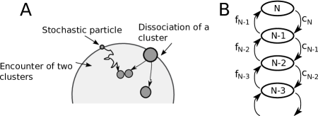
Figure 1: (A) Coagulation-fragmentation of a finite number of particles. Two particles aggregate at a rate $k_{f}$ and a cluster of $n$ splits at a rate $(n-1)k_{b}$. (B) The Markov chain representation of the cluster dynamics where $f_{K}$ (resp. $c_{K}$) is the dissociation (resp. association) rate of a cluster (resp. of two clusters) when there are $K$ clusters.

To determine the number of clusters at steady state, we integrate explicitly the Markov chain (LABEL:Markov1) and the steady state probability $\Pi_{K}=\lim_{t\rightarrow\infty}P_{K}(t)$ is given by

$$\Pi_{K+1}=\frac{(2a)^{K}}{K!}\frac{(N-1)!}{(K+1)!(N-K-1)!}\Pi_{1},$$ (10)

where the equilibrium parameter is

$$a=\frac{k_{b}}{k_{f}}.$$ (11)

Using the normalization condition $\sum_{K}\Pi_{K}=1$, the probability $\Pi_{1}$ can be expressed using hypergeometric series:

$$\Pi_{1}=\frac{1}{{}_{1}F_{1}(-N+1;2;-2a)},$$ (12)

where ${}_{1}F_{1}$ is the Kummer’s confluent hypergeometric function (Eq. 13.1.2, [10]). At steady state, the average number of clusters is

$$<M_{\infty}(a,N)>=\sum_{K=1}^{N}K\Pi_{K}=1+a(N-1)G_{1}(a,N)$$ (13)

where

$$G_{1}(a,N)=\frac{{}_{1}F_{1}(-N+2;3;-2a)}{{}_{1}F_{1}(-N+1;2;-2a)}.$$ (14)

In addition, the $n$th-order moment $\mu_{n}$ is given by

$$\mu_{n}=\sum K^{n}\Pi_{K}=\frac{H^{n}({{}_{1}F_{1}})(-N+1;2;z)_{|z=-2a}}{{}_{1}F_{1}(-N+1;2;-2a)},$$ (15)

where $H$ is the operator defined by $H(f)(z)=\frac{d}{dz}zf(z)$. Since the derivative of Kummer’s function is

$$\frac{d{{}_{1}F_{1}}(\alpha;\beta;z)}{dz}=\frac{\alpha}{\beta}{{}_{1}F_{1}}(\alpha+1;\beta+1;z),$$ (16)

the moments can be written as

$$\mu_{n} = \sum_{k=0}^{n}\alpha_{k}^{n}\frac{(N-1)!}{(k+1)!(N-1-k)!}\frac{(2a)^{k}}{k!}G_{k}(a,N),$$

$$= \sum_{k=0}^{n}\alpha_{k}^{n}\frac{\Pi_{k+1}}{\Pi_{1}}G_{k}(a,N),$$

where

$$G_{n}(a,N)=\frac{{}_{1}F_{1}(-N+1+n;2+n;-2a)}{{}_{1}F_{1}(-N+1;2;-2a)}$$ (17)

and the coefficients $\alpha_{k}^{n}$ are given by

$$\alpha_{k}^{n}=\left\{\begin{array}[]{ccc}k!\sum_{j=0}^{k/2}(-1)^{j}\displaystyle{\frac{(k+1-j)^{n}+(j+1)^{n}}{(k-j)!}}\mbox{ if $k$ is even,}\\ \\ k!\sum_{j=0}^{(k-1)/2}(-1)^{j}\displaystyle{\frac{(k+1-j)^{n}-(j+1)^{n}}{(k-j)!}}\mbox{ if $k$ is odd,}\\ \end{array}\right.$$ (21)

and $\alpha_{0}^{n}=\alpha_{n}^{n}=1$. Thus the variance of the number of clusters is given by

$$<V_{\infty}(a,N)> = \mu_{2}-\mu_{1}^{2}$$ (22)

$$= a(N-1)G_{1}(a,N)+\frac{2}{3}a^{2}(N-1)(N-2)G_{2}(a,N)-a^{2}(N-1)^{2}G_{1}^{2}(a,N).$$

In addition, for large $N$ and fixed $a$, using asymptotic results for hypergeometric functions [10], we have

$$G_{n}(a,N) \approx \frac{(n+1)!}{(2aN)^{n/2}},$$ (23)

and we obtain from equation (13) that the mean number of clusters is

$$<M_{\infty}(a,N)>=\sqrt{2aN}+O(1).$$ (24)

As a result of the above analysis, we can estimate the mean number of clusters $<M_{\infty}(a,N)>$, which is plotted as a function of $a$ (Fig. 2A) and $N$ (Fig. 2B).

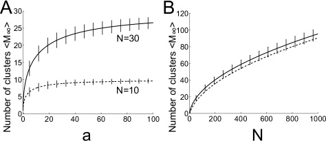
Figure 2: Number of clusters $<M_{\infty}(a,N)>$ as a function of the equilibrium parameter $a$ (A), for $N=10$ and $N=30$ obtained from eq. (13) and (B) as a function of number $N$ for $a=5$, using eq. (13) (continuous line) and the asymptotic approximation eq. (24) (dashed line).

3 Size of the clusters

Because the previous analysis cannot predict the size of the clusters, we shall now evaluate the probability density function for the number of clusters of different sizes. This analysis relies on carefully studying the configurations of $N$ particles decomposed in $K$ clusters. The configuration is described by the ensemble of ordered clusters of size $n_{1},\dots,n_{K}$

$$A_{N,K}=\{(n_{j})_{1\leq j\leq K};\sum_{i=1}^{K}n_{i}=N\mbox{, }n_{1}\geq\dots\geq n_{K}\geq 1\},$$

which is equivalent to the set

$$A_{N,K}^{\prime}=\{(m_{i})_{1\leq i\leq N};\sum_{i=1}^{N}im_{i}=N\mbox{, }\sum_{i=1}^{N}m_{i}=K\},$$

where $m_{i}$ is the number of clusters of size $i$. The correspondence from $A_{N,K}$ to $A_{N,K}^{\prime}$ is obtained by taking into account that for all clusters $n_{j}$ of size $i$, we have the relation $m_{i}=\sum_{j}\mathbb{I}(n_{j}=i)$ [2]. We enumerate the number of configurations associated with the ensemble $A_{N,K}^{\prime}$. It is the same as counting the occurrence of the integer $i$ in the decomposition of $N$ as a sum of $K$ integers. The number of occurrence of the configuration $(m_{1},\dots,m_{N})$, when there are $m_{1}$ clusters of size 1, $m_{2}$ clusters of size 2 …, is the multinomial coefficient $\frac{K!}{m_{1}!\dots m_{N}!}$. Thus the conditional probability of the $(m_{1},\dots,m_{N})$ distribution, when the total number of clusters is equal to $K$, is obtained by normalizing the equilibrium over all possibilities

$$p(m_{1},\dots,m_{N}|K)=\frac{\displaystyle{\frac{K!}{m_{1}!\dots m_{N}!}}}{\sum_{(m_{i})\in A_{N,K}^{\prime}}\displaystyle{\frac{K!}{m_{1}!\dots m_{N}!}}}.$$ (25)

Interestingly by summing the series $(X+X^{2}+...+X^{N})^{K}$ for the $N^{th}$ order coefficient and using the $N-K$ derivative of $\frac{1}{(1-X)^{K}}$, we have

$$\sum_{(m_{i})\in A_{N,K}^{\prime}}\displaystyle{\frac{K!}{m_{1}!\dots m_{N}!}}=\frac{(N-1)!}{(K-1)!(N-K)!}.$$ (26)

At this stage, we shall explain the rational for expression (25). Indeed, it corresponds to the equilibrium distribution of particles in clusters, where the dissociation (resp. association) rate is proportional to the number of elements (minus one) (resp. the number of pairs of particles).

This consideration defines the steady state. Indeed, if we consider the equilibrium probability distributions associated with the Markov chain configuration $(m_{1},\dots,m_{N})$, then the transition between the two neighboring states $(m_{1},\dots,m_{i}-1,\dots,m_{j}-1,\dots,m_{i+j}+1,\dots,m_{N})$ and $(m_{1},\dots,m_{N})$, is obtained first from the coagulation of a cluster of size $i$ with one of size $j$, with a rate $C(i,j)=\frac{k_{f}}{2}m_{i}m_{j}$ if $i\neq j$ and $C(i,i)=\frac{k_{f}}{2}m_{i}(m_{i}-1)$ otherwise. The factor $\frac{1}{2}$ accounts for the two cases $C(i,j)$ and $C(j,i)$. The fragmentation rate from $i+j$ to $(i,j)$ is $F(i,j)=k_{b}(m_{i+j}+1)$ (Fig. 3). Thus, the stationary probability $\pi$ necessarily satisfies the relation

$$\frac{\pi(m_{1},\dots,m_{i}-1,\dots,m_{j}-1,\dots,m_{i+j}+1,\dots,m_{N})}{\pi(m_{1},\dots,m_{N})}=\frac{C(i,j)}{F(i,j)}=\frac{1}{2a}\frac{m_{i}m_{j}}{m_{i+j}+1}.$$ (27)

When the configuration $(m_{1},\dots,m_{N})$ is made of $K$ clusters, the configuration $(m_{1},\dots,m_{i}-1,\dots,m_{j}-1,\dots,m_{i+j}+1,\dots,m_{N})$ has $K-1$ clusters. From Eq. (5), we have that

$$\Pi_{K-1}(a)=\Pi_{K}(a)\frac{K(K-1)}{2(N-K+1)a}$$

and the conditioned stationary probability satisfies

$$\frac{\pi(m_{1},\dots,m_{i}-1,\dots,m_{j}-1,\dots,m_{i+j}+1,\dots,m_{N})|K-1)}{\pi(m_{1},\dots,m_{N}|K)} = \frac{\Pi_{K}(a)}{\Pi_{K-1}(a)}\frac{1}{2a}\frac{m_{i}m_{j}}{m_{i+j}}$$ (28)

$$= \frac{N-K+1}{K(K-1)}\frac{m_{i}m_{j}}{m_{i+j}+1}.$$ (29)

A direct computation shows that the probability $p(m_{1},\dots,m_{N})$ satisfies equation (29) [11].

Figure 3: Markov chain representation of the configuration dynamics. When the configuration is $(m_{1},\dots,m_{N})$, the dissociation rate of a cluster of size $i$ into a cluster of size $k$ and one of size $i-k$ is $k_{b}m_{i}$, while the rate of formation of a cluster of size $i+j$ from two clusters of size $i$ and $j$ is equal to $\frac{k_{f}}{2}m_{i}m_{j}$.

Now using Bayes rule, the joint probability of the configuration $(m_{1},\dots,m_{N})$ and $K$ clusters is the product of the conditional probability $p(m_{1},\dots,m_{N}|K)$ by the probability of having $K$ clusters

$$p(m_{1},\dots,m_{N},K)=p(m_{1},\dots,m_{N}|K)\Pi_{K}.$$ (30)

We shall now estimate the size of clusters from the above considerations. For a total of $N$ particles, when there are $K$ clusters, the mean number of clusters of size $n$ is

$$<M_{n}>_{K} = \sum_{(m_{i})\in A_{N,K}^{\prime}}m_{n}p(m_{i}|K)$$

$$= \frac{(N-n-1)!K!(N-K)!}{(N-1)!(K-2)!(N-n-K+1)!},$$

which we computed using equation (26) and that when a cluster of size $n$ is contained in the distribution $(m_{1},\dots,m_{N})$, it is equivalent to have $N-n$ particles in $K-1$ clusters. Finally the mean number of clusters of size $n$ is obtained by summing over all possibilities when there are $K$ clusters,

$$<M_{n}> = \sum_{K=1}^{N}<M_{n}>_{K}\Pi_{K}$$

$$= \frac{(N-n-1)!}{(N-1)!}\sum_{K}\frac{K(K-1)(N-K)!}{(N-n-K+1)!}\Pi_{K}.$$

Using the expression for $\Pi_{K}$ (10), we obtain

$$\left\{\begin{array}[]{ccc}<M_{n}>&=&2a\displaystyle{\frac{{{}_{1}F_{1}}(-N+1+n;2;-2a)}{{{}_{1}F_{1}}(-N+1;2;-2a)}}\mbox{ if }n<N,\\ &&\\ <M_{N}>&=&\displaystyle{\frac{1}{{{}_{1}F_{1}}(-N+1;2;-2a)}}.\\ \end{array}\right.$$ (35)

In addition, the mean number of clusters of size $n$ is $2a\frac{\Pi_{1}(N)}{\Pi_{1}(N-n)}$, i.e. this is the probability ratio of having one cluster when there are $N$ particles over the probability of having one cluster when there are $N-n$ particles. Finally, the variance of the number of clusters of size $n$ is, if $N>2n+1$,

$$<V_{n}> = <M_{n}>-<M_{n}>^{2}+2a\frac{N-2n-1}{(N-2n+1)(N-2n+2)}\times\bigg{(}\frac{\Pi_{1}(N)}{\Pi_{1}(N-2n)}-\frac{\Pi_{1}(N)}{\Pi_{1}(N-2n-1)}\bigg{)}$$ (36)

and otherwise

$$<V_{n}> = <M_{n}>-<M_{n}>^{2}.$$ (37)

To summarize this analysis, we plot in Fig. 4 the mean number of clusters of size $n$ for five particles. We will also use this analysis in the final section to study telomere clustering in yeast.

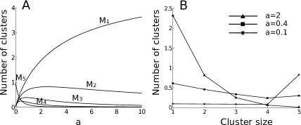
Figure 4: Mean number $<M_{n}>$ of clusters of size $n$ as a function of the parameter $a$ (A) for $N=5$ particles (equation (35)) and (B) mean number of cluster for $a=0.1$, $a=0.4$ and $a=2$ as a function of the cluster size.

At equilibrium, particles are exchanged between clusters. To characterize the exchange of telomeres between clusters, we now estimate the probability $p_{2}(N,a)$ to have two given particles in the same cluster $C$ for a fixed number of particles $N$ and equilibrium constant $a$. For a distribution of clusters $(n_{1},\dots,n_{K})$, the probability for two specific particles to be in $C$ is obtained by choosing the first particle in the cluster $n_{i}$, which is equal to the number of particles in the cluster divided by the total number of particles $\frac{n_{i}}{N}$ and thus the probability to have the second particle in the same cluster is $\frac{n_{i}-1}{N-1}$. Summing over all clusters, we get

$$P(2\hbox{ particles }\in C|(n_{1},..n_{K})) = \sum_{i=1}^{K}\frac{n_{i}}{N}\frac{n_{i}-1}{N-1}$$

$$= \frac{1}{N(N-1)}(\sum_{i=1}^{K}n^{2}_{i}-N).$$

Using that $\sum_{j=1}^{N}n_{j}^{2}=\sum_{i=1}^{N}i^{2}m_{i}$, we have

$$\sum_{(n_{j})\in A_{N,K}}p(n_{j})\sum_{j=1}^{K}n^{2}_{j}=N+2N\frac{N-K}{K+1}.$$ (39)

Summing now over all distributions of clusters, the probability

$$p_{2}(N,a)=-\frac{2}{N-1}+\frac{N+1}{N-1}\frac{{}_{1}F_{1}(-N+1;3;-2a)}{{}_{1}F_{1}(-N+1;2;-2a)}.$$ (40)

Surprisingly, the three-term recurrence relation for Kummer’s function ([10] Eqs. 13.4.1-13.4.6) gives ${}_{1}F_{1}(-N+1;3;-2a)=\frac{N-1}{N+1}{{}_{1}F_{1}}(-N+2;3;-2a)+\frac{2}{N+1}{{}_{1}F_{1}}(-N+1;2;-2a).$ Finally

$$p_{2}(N,a)=G_{1}(a,N).$$ (41)

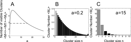
Figure 5: (A) Number of clusters containing more than three particles $O(N,a)$ as a function of the equilibrium parameter $a$, for $N=32$. Experimentally, 2.9 clusters were observed in average, which corresponds to $a=0.2$ and $a=15$. (B, C) Distribution of the mean number of clusters as a function of the cluster size (Eq. (35)), for $N=32$ and $a=0.2$ (B) and $a=15$ (C). Grey bars indicate single particles and clusters of two particles, which are not observable.

4 Application to telomere clustering in yeast

To apply the previous analysis to the organization of telomere clustering in yeast, we use a coarse-grained model of a telomere, the motion of which can be approximated as Brownian [12]. In addition, because clusters are of small sizes, the arrival time of a telomere to cluster is Poissonnian. Indeed, it is the time for a stochastic particle moving on the nuclear surface to reach a small target. Our goal is now to show that telomere clustering can be described by our diffusion-fragmentation-association model and thus by the Master equation (LABEL:Markov1). For that purpose, we propose to estimate the forward and backward rates, constrained by recent observations that in yeast the 32 telomeres form 2 to 8 clusters, with an average of 2.9 clusters per cell, containing in average 4 telomeres [13, 14].

For a telomere radius $r=0.015$ $\mu$m, moving on a sphere (nucleus surface) of radius $R=1$ $\mu$m with a diffusion coefficient $D=0.005$ $\mu$m².s^-1 [15], we find using a Brownian simulation for two telomeres to meet, that the forward rate is $k_{f}=1.910^{-3}$ s^-1. Although the cluster can vary in size when telomeres attach, we shall make the assumption that the encounter will stay constant and use this rate in our previous Markov modeling. Indeed, telomeres are attached to the nuclear surface by a family of proteins Sir2/Sir3/Sir4 [13, 14]. Telomere clusters are elicited by the formation of Sir3-Sir3 interactions, and Sir3 abundance is directly related to the stability of the clusters (dissociation rate $k_{b}$). Thus, in the absence of any experimental evidences, we consider that telomere diffusion is driven by a molecular complex, moving on the nuclear surface. When this complex has the shape of a cylinder, the diffusion constant is given by the log of the radius [16]. Since clusters contain at most four telomeres [14], the effective radius does not change much leading to a small change of the diffusion constant. This justifies our constant approximation for the encounter rate $k_{f}(m,n)$ of two clusters of size $n$ and $m$.

The dissociation rate $k_{b}$ of a telomere from a cluster cannot be easily derived from experimental data because clusters made of one or two telomeres are not experimentally visible [14]. Using the results of the first sections (equations (13),(35)), we use our model Markov model to compute and to plot (Fig. 5A) the number of visible clusters obtained by the formula

$$O(N,a) = <M_{\infty}(a,N)>-<M_{1}(a,N)>-<M_{2}(a,N)>$$

$$= 1-4a+(a(N-1)+6a^{2})G_{1}(a,N)-\frac{4}{3}a^{3}G_{2}(a,N)$$

as a function of the equilibrium parameter $a$. We find from this graph that there are two possible values for $a$, giving an average of 2.9 visible clusters, which are $a=0.2$ and $a=15$. To select the correct value, we built the cluster distributions associated for these two values from equations (35). We further obtained the mean number of clusters of a given size (Fig. 5B,C). However, for $a=0.2$, telomeres form a giant cluster, containing almost all the telomeres, which is not reported experimentally. Finally, we conclude that $a=15$, for which there are always less than five telomeres per cluster, in agreement with experimental observations [14]. Furthermore, we obtain for the dissociation rate, the value $k_{b}=ak_{f}=0.03$ s^-1, which was not known before. Finally, using formula (41), we can predict that two specific telomeres are located in the same cluster approximately 4% of the time.

In conclusion, we obtained here a novel analysis for a coagulation-fragmentation process of a finite number of Poissonnian particles restricted in a bounded domain. We used our model to estimate the dissociation rate $k_{b}$ of telomeres from a cluster, a constant that can reveal the local organization of telomeres in a cluster. Although we applied this analysis to the organization of telomeres in yeast, it could be applied to study telomere organization for general organisms.

References

- [1] A. Lushnikov, Izv. Akad. Nauk SSSR, Ser. Fiz. Atmosfer. I Okeana, 14, (1978) 738-743.
- [2] J. Pitman, Combinatorial Stochastic Processes, École d’Été de Probabilités de Saint-Flour XXXII. Lecture Notes in Math. 1875. Springer, Berlin
- [3] M. von Smoluchowski, Physik. Zeit. 17 (1916) 557-585.
- [4] M. Bramson, J. L. Lebowitz, Phys. Rev. Lett. 61, (1988) 2397-2400.
- [5] C.R. Doering, D. Ben-Avraham. Phys. Rev. Lett. 62, (1989) 2563-2566.
- [6] J.A.D. Wattis, Physica D 222, (2006) 1-20.
- [7] S. Redner, A Guide to First-Passage Processes, (Cambridge University Press, 2001).
- [8] Z. Schuss, Diffusion and Stochastic Processes: an Analytical Approach, (Springer New York, 2010).
- [9] B.J. Matkowsky, Z. Schuss, C. Knessl, C. Tier, M. Mangel. Phys. Rev. A 29, (1984) 3359.
- [10] M. Abramowitz, I.A. Stegun, Handbook of Mathematical Functions, (Dover Publications, 1972)
- [11] R. Durrett, B. Granovsky, S. Gueron. J. Theor. Probability 12, (1999) 447-474.
- [12] I. Bronstein, Y. Israel, E. Kepten, S. Mai, Y. Shav-Tal, E. Barkai, Y. Garini, Phys. Rev. Lett. 103, (2009) 018102.
- [13] M. Gotta, T. Laroche, A, Formenton, L. Maillet, H. Scherthan, S.M. Gasser, J. Cell Biol. 134, (1996) 1349-1363.
- [14] M. Ruault, A. De Meyer, I. Loiodice, A. Taddei, J. Cell Biol. 192, (2011) 417-431.
- [15] K. Bystricky, P. Heun, L. Gehlen, J. Langowski, S.M. Gasser, Proc. Natl. Acad. Sci. U.S.A. 101, (2004) 16495-16500.
- [16] P.G. Saffman, M. Delbrück, Proc. Natl. Acad. Sci. U. S. A. 72, (1975) 3111-3113.