Magnetoexcitons and optical absorption of bilayer-structured topological insulators

Abstract

The optical absorption properties of magnetoexcitons in topological insulator bilayers under a strong magnetic field are theoretically studied. A general analytical formula of optical absorption selection rule is obtained in the noninteracting as well as Coulomb intra-Landau-level interacting cases, which remarkably helps to interpret the resonant peaks in absorption spectroscopy and the corresponding formation of Dirac-type magnetoexcitons. We also discuss the optical absorption spectroscopy of magnetoexcitons in the presence of inter-Landau-level Coulomb interaction, which becomes more complex. We hope our results can be detected in the future magneto-optical experiments.

The bilayer $n$-$p$ systems, comprising electrons from the $n$ layer and holes from the $p$ layer, have been the subject of recent theoretical and experimental investigations in low-dimensional condensed matter physics. The coupled quantum wells Snoke ; Butov ; Timofeev ; Eisenstein and layered graphene Zhang ; Min ; Lozovik1 ; Iyengar ; Berman ; Berman1 ; Koinov are of particular interest in connection with the possibility of the Bose-Einstein condensation and superfluidity of indirect excitons or electron-hole pairs. On the other hand, as a new state of quantum matter, topological insulators (TIs) Kane2005 ; Bernevig ; Fu2007 ; Konig ; Hsieh ; Moore ; Hasan ; Qi ; Qi2 are now being in intensive study. They are characterized by a full insulating gap in the bulk and topologically protected gapless edge or surface states in low dimensions, in which by their single-Dirac-point nature it is highly desirable to find stable and intriguing electron-hole excitations.

With the rapid progress in advanced nanotechnology, it is possible to fabricate a bilayer $n$-$p$ system with TIs. We call this system as “topological insulator bilayer (TIB)”, which comprises two TI thin films separated by a dielectric barrier. The schematic scheme is shown in Fig. 1(a). Bi₂Se₃-family materials are one of the best candidates for their large bulk-gap width Zhang2009 ; Xia2009 ; Chen2009 . In order to form steady excitons or magnetoexcitons, the dielectric spacer can be chosen from those with small dielectric constant, such as Al₂O₃ and SiO₂, on which, remarkably, high-quality TI quantum well thin films have been now successively grown Chang ; Li ; Liu ; Aguilar . By doping or applying external gates, electron and hole carriers will form in both topological insulator thin films, which behave like massless Dirac particles. However, these quasiparticles can not form excitons because there is no gap opening. To produce a gap we apply a strong perpendicular magnetic field on the TIB. In this case, the Dirac-type energy spectrum of these quasiparticles becomes discrete by forming Landau levels (LLs), which results in the possible formation of magnetoexcitons in this system.

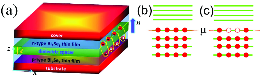
Figure 1: (Color online) (a) Scheme of TIB consisting of two Be₂Se₃ thin films separated by dielectric spacer. Electron (hole) carriers are induced by $n$($p$)-type doping or applied external gates. Indirect magnetoexcitons can be formed in presence of strong external magnetic field. (b) and (c) are schematic representations of the chemical potential location. (b) represents the fully occupied case and (c) represents the partially occupied case.

The optical absorption spectroscopy analysis is an instructive method in studying the properties of magnetoexcitons, because it can provide the knowledge of magnetoexciton’s energies and wavefunctions at $\mathbf{P}$=$0$, where $\mathbf{P}$ is the magnetoexciton momentum. Many efforts have been devoted to exploring the optical absorption properties of magnetoexciton in semiconductor quantum wells by using the magneto-optical measurements Marquezini ; Kim2004 . More recently, the optical characterization of Bi₂Se₃ in a magnetic field has been experimentally studied LaForge2010 . Based on this, the main purpose of the present paper is to study the magnetoexciton’s optical absorption spectroscopy in TIBs. Note that the magneto-optical response of Bi₂Se₃ thin film grown on dielectric substrate has recently been experimentally measured Aguilar . Through applying a strong magnetic field, the Coulomb interaction (CI) between electrons in the upper TI film and holes in the lower TI film can be thought as a perturbation compared to the energy difference between LLS. For convenience, we divide the CI perturbation into the intralevel [see the following text and Eq. (10)] and interlevel parts. Firstly, we consider a simple case in which only the intralevel CI is introduced. In this case, we deduce a general analytical formula for magnetoexciton’s optical absorption selection rule. According to this selection rule, one can clearly point out which magnetoexciton corresponds to the specific resonant peaks in absorption spectroscopy. Then, we study the case in which interlevel component of CI is also included. In this case, the optical absorption spectroscopy becomes more complex and intriguing by the mixing of the excitations.

We start with the effective Hamiltonian of TIB system $\mathcal{H}$=$H_{0}\mathtt{+}U(\mathbf{r})$, where

$$H_{0}=v_{F}\mathbf{\sigma}_{e}\cdot\left(\mathbf{\hat{z}}\times\mathbf{\pi}_{e}\right)-v_{F}\mathbf{\sigma}_{h}\cdot\left(\mathbf{\hat{z}}\times\mathbf{\pi}_{h}\right)$$ (1)

is the free electron-hole part of TIB, while $U(\mathbf{r})$=$-e^{2}/\epsilon\sqrt{|\mathbf{r}|^{2}+d^{2}}$ is the CI between the pair of electron and hole with $\mathbf{r}\mathtt{=}\mathbf{r}_{e}\mathtt{-}\mathbf{r}_{h}$ the relative coordinate in the $x$-$y$ plane and $d$ the spacer thickness. Here, $\mathbf{r}_{e(h)}$ represents the position of the electron (hole), and $\mathbf{\pi}_{e(h)}$ =$\mathbf{p}_{e(h)}\mathtt{\pm}e\mathbf{A}_{e(h)}/c$=$-i\partial/\partial\mathbf{r}_{e(h)}\mathtt{\pm}e\mathbf{A}_{e(h)}/c$ denotes the in-plane momentum of the electron (hole), where the gauge is chosen as $\mathbf{A}_{e(h)}$=$B(0,x_{e(h)},0)$ in the following calculations. $v_{F}$ is the Fermi velocity ($\mathtt{\sim}3\mathtt{\times}10^{5}$ m/s for Bi₂Se₃-family materials LiuCX ; Wangzg ), $\mathbf{\hat{z}}$ is the unit vector normal to the surface, and $\mathbf{\sigma}_{e}\mathtt{=}$ $\mathbf{\sigma}\otimes\mathbb{I}$ ($\mathbf{\sigma}_{h}\mathtt{=}$ $\mathbb{I}$ $\mathtt{\otimes}$ $\mathbf{\sigma}$) describes the spin operator acting on the electron (hole), in which $\mathbf{\sigma}$ denotes a vector of Pauli matrices and $\mathbb{I}$ is the 2$\times$2 identity matrix.

The eigenstates of Hamiltonian $H_{0}$ have the form

$$\psi_{\mathbf{P}}\left(\mathbf{R},\mathbf{r}\right)\mathtt{=}\exp\left[i\left(\mathbf{P}\mathtt{+}\frac{e}{2c}\left[\mathbf{B}\mathtt{\times}\mathbf{r}\right]\right)\mathtt{\cdot}\mathbf{R}\right]\Psi\left(\mathbf{r}\mathtt{-}\mathbf{r}_{0}\right),$$ (2)

where $\mathbf{R}$=($\mathbf{r}_{e}\mathtt{+}\mathbf{r}_{h}$)$/2$, $\mathbf{r}$=$\mathbf{r}_{e}\mathtt{-}\mathbf{r}_{h}$, and $\mathbf{r}_{0}$=$l_{B}^{2}$($\mathbf{\hat{B}}\mathtt{\times}\mathbf{P}$) with $l_{B}$ being the magnetic length. For an electron in LL $n_{+}$ and a hole in LL $n_{-}$, the four-component wave functions for the relative coordinate are given by Iyengar

$$\Psi_{n_{+},n_{-}}(\mathbf{r})=|n_{+},n_{-}\rangle$$ (3)

$$=(\sqrt{2})^{\delta_{n_{+},0}+\delta_{n_{-},0}-2}\left(\begin{array}[c]{c}\Phi_{|n_{+}|-1,|n_{-}|-1}(\mathbf{r})\\ i^{-\text{sgn}(n_{-})}\Phi_{|n_{+}|-1,|n_{-}|}(\mathbf{r})\\ i^{\text{sgn}(n_{+})}\Phi_{|n_{+}|,|n_{-}|-1}(\mathbf{r})\\ i^{\text{sgn}(n_{+})-\text{sgn}(n_{-})}\Phi_{|n_{+}|,|n_{-}|}(\mathbf{r})\end{array}\right),$$ (8)

where $\Phi_{n_{1},n_{2}}(\mathbf{r})\mathtt{=}\frac{2^{-\frac{|l_{z}|}{2}}n_{\_}!e^{-il_{z}\phi}\delta\left(l_{z}\right)r^{|l_{z}|}}{\sqrt{2\pi n_{1}!n_{2}!}}L_{n_{-}}^{|l_{z}|}(\frac{r^{2}}{2})e^{-\frac{r^{2}}{4}}$ with $l_{z}$=$n_{1}\mathtt{-}n_{2}$, $n_{-}\mathtt{=}\min(n_{1},n_{2})$, and $\delta\left(l_{z}\right)$=sgn$(l_{z})^{l_{z}}\mathtt{\rightarrow}1$ for $l_{z}$=$0$. The corresponding LLs are given by

$$E_{n_{+},n_{-}}^{(0)}\mathtt{=}\frac{\sqrt{2}v_{F}}{l_{B}}\mathtt{[}\text{sgn}(n_{+})\sqrt{|n_{+}|}\mathtt{-}\text{sgn}(n_{-})\sqrt{|n_{-}|}\mathtt{].}$$ (9)

Taking CI as a perturbation in the first order and only considering its intralevel component, the energy dispersion of magnetoexcitons can be easily obtained as

$$E_{n_{+},n_{-}}\mathtt{=}E_{n_{+},n_{-}}^{(0)}\mathtt{+}\langle\Psi_{n_{+},n_{-}}|U\left(\mathbf{r}\mathtt{+}\mathbf{r}_{0}\right)|\Psi_{n_{+},n_{-}}\rangle.$$ (10)

However, to take into account the interlevel CI, we should perform diagonalization of the full Hamiltonian for Coulomb interacting carriers in some basis of magnetoexciton states $\Psi_{n_{+},n_{-}}(\mathbf{r})$. To obtain eigenvalues of the Hamiltonian $\mathcal{H}$, we need to solve the following equation:

$$0 \mathtt{=}\det\left\|\delta_{n_{+},n_{+}^{\prime}}\delta_{n_{-},n_{-}^{\prime}}(E_{n_{+},n_{-}}^{(0)}\mathtt{-}E)\right.$$ (11)

$$\left.\mathtt{+}\langle\Psi_{n_{+}^{\prime},n_{-}^{\prime}}|U\left(\mathbf{r}\mathtt{-}l_{B}^{2}\mathbf{\hat{z}}\mathtt{\times}\mathbf{P}\right)|\Psi_{n_{+},n_{-}}\rangle\right\|.$$

The location of the chemical potential will determine the possible LL indices for electrons and holes. For convenience, in this paper we use the notation $\mu$ for the highest filled LL and only consider two cases: (i) Electron LLs with $n_{+}$$>$$\mu$ are unoccupied and hole LLs with $n_{-}\mathtt{\leqslant}\mu$ are fully occupied and (ii) electron LLs with $n_{+}\mathtt{>}\mu$ are unoccupied and hole LLs with $n_{-}\mathtt{<}\mu$ are fully occupied, while the LL at $\mu$ is partially occupied. These two cases are schematically represented in Fig. 1(b) and 1(c), respectively. To distinguish these two cases, in the following discussion we call the first case as fully occupied case and the second one as partially occupied case.

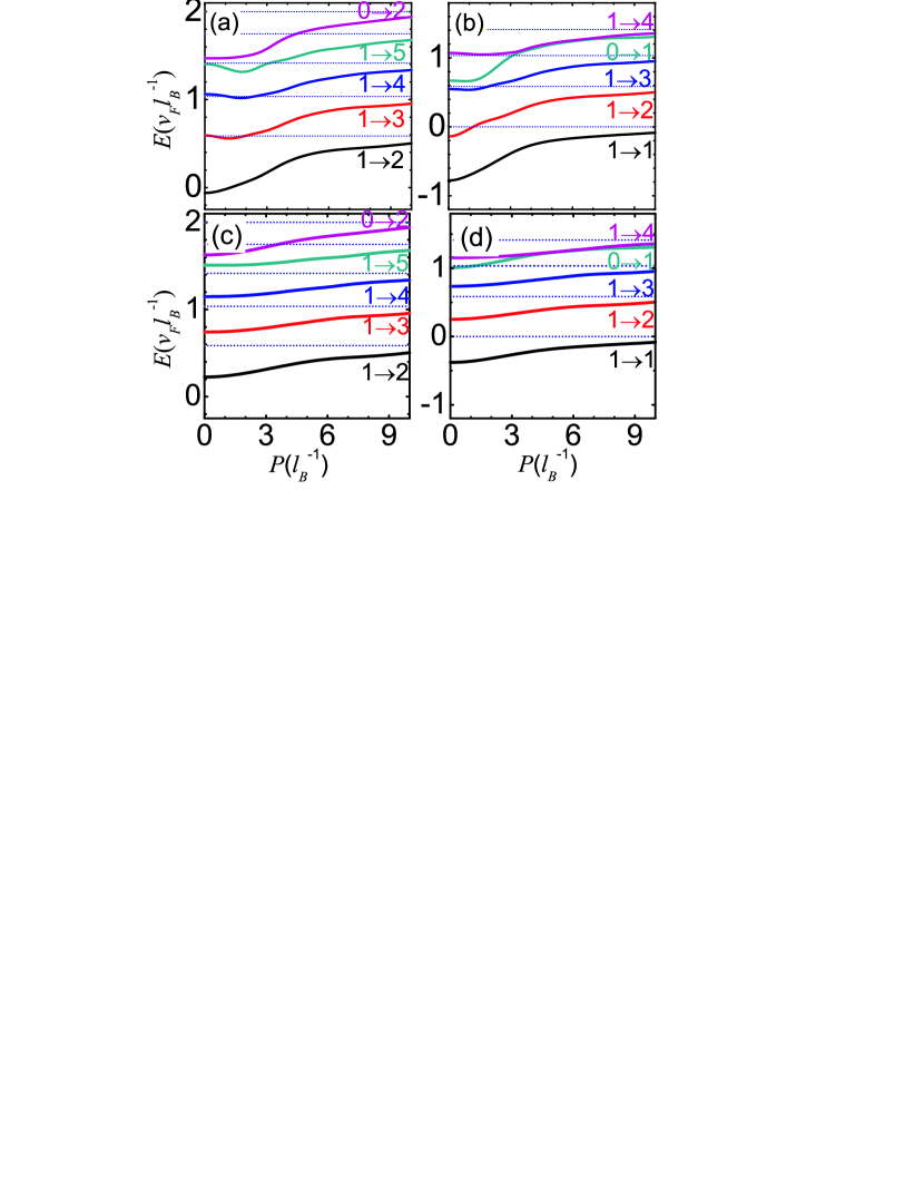
Figure 2: (Color online) Energy dispersion of the first five magnetoexciton LLs for the fully (left panels) and partially (right panels) occupied cases. $\beta$=$0.9$ and $\mu$=$1$. The spacer thickness $d$=$0.2l_{B}$ for (a) and (b), while $d$=$2.0l_{B}$ for (c) and (d).

We take $\mu$=$1$ as an example to numerically solve Eq. (11) by employing five electron and five hole levels. In our calculations we use the notation $\beta\mathtt{\equiv}\left(e^{2}/\epsilon l_{B}\right)/(v_{F}/l_{B})=e^{2}/\left(\epsilon v_{F}\right)$ to describe the relative CI strength. Figures 2(a) and 2(b) plot the first five energy levels as a function of $P$ for fully and partially occupied cases, respectively. Here, the spacer thickness is chosen to be $d$=$0.2l_{B}$. With increasing $d$, the CI effect turns to become faint. As a result, the magnetoexciton’s energy levels become smoother. This can be clearly seen from Figs. 2(c) and 2(d), where the spacer thickness $d$=$2.0l_{B}$ is used for comparison with cases of $d$=$0.2l_{B}$.

Let us now turn to discuss the optical absorption properties of magnetoexcitons with $P=0$. The magneto-optical experiments provides a good method to detect the magnetoexcitons since the particle-hole excitation energy could be determined directly by the resonant peaks in the optical conductivity. Up to this stage, the LLs have been assumed to be sharp, and thus from Fermi’s golden rule, the optical absorption for photons of frequency $\omega$ yields a sum of delta functions in energy,

$$R(\omega)\text{=}\frac{2\pi}{\hslash}\sum_{\alpha}\left|\langle\alpha|\frac{e}{c}\mathbf{A}\cdot\mathbf{v}|0\rangle\right|^{2}\delta(\epsilon_{eh}^{(\alpha)}-\hslash\omega),$$ (12)

where $\alpha$ is the set of quantum numbers describing a particle-hole excitation and $|0\rangle\mathtt{\equiv}|\mu,\mu\rangle$ is the ground state in absence of particle-hole excitations. $\mathbf{v}$=$\partial\mathcal{H}_{0}/\hslash\partial\mathbf{k}$ is the velocity operator for non-interacting electrons (we neglect the renormalization of the Fermi velocity due to interactions). $\mathbf{A}$ is the vector potential. For linear polarized light $\mathbf{A}$=$A\mathbf{\hat{x}}$, one easily deduce $v_{x}\mathtt{\varpropto}m_{x}^{-}$=($\sigma_{e}^{y}$-$\sigma_{h}^{y}$)$/2$.

For the purpose of resolving the spatial functional forms and reflecting realistic experimental conditions one should either assume that the LLs are broadened or that the magnetoexciton has a finite lifetime. We choose, therefore, a Lorentzian type broadening $\delta(\epsilon_{eh}^{(\alpha)}\mathtt{-}\hslash\omega)\mathtt{\rightarrow}\frac{\gamma/2}{(\epsilon_{eh}^{(\alpha)}-\omega)^{2}+\gamma^{2}/4}$ with linewidth $\gamma$ in following calculations. Substituting it into Eq. (12), one gets

$$R(\omega)\mathtt{\varpropto}\sum_{\alpha}\left|\langle\alpha|m_{x}^{-}|0\rangle\right|^{2}\frac{\gamma/2}{(\epsilon_{eh}^{(\alpha)}\mathtt{-}\omega)^{2}\mathtt{+}\gamma^{2}/4}$$ (13)

with $\left|\langle\alpha|m_{x}^{-}|0\rangle\right|^{2}\mathtt{=}\sum_{n_{+}>\mu}\sum_{n_{-}\leqslant\mu}\int Td\mathbf{r}$ for full occupation and $\sum_{n_{+}\geqslant\mu}\sum_{n_{-}\leqslant\mu}\int Td\mathbf{r}$ for partial occupation. The parameter $T$ is defined as

$$T\mathtt{=}|C_{n_{+},n_{-}}^{\alpha}\langle n_{+},n_{-}|m_{x}^{-}|\mu,\mu\rangle|^{2},$$ (14)

where $C_{n_{+},n_{-}}^{\alpha}$ is the projection of magnetoexciton state $\alpha$ on the basis state $|n_{+},n_{-}\rangle$.

Let us now consider a simple case in which only the intralevel CI is considered. This case is similar to that without CI, in which the magnetoexciton state $\alpha$ is one special basis state and $C_{n_{{}_{+}},n_{{}_{-}}}^{\alpha}$=$\delta_{\alpha,(n_{{}_{+}},n_{{}_{-}})}$. So by substituting Eq. (3) into $\langle n_{+},n_{-}|m_{x}^{-}|\mu,\mu\rangle$, we can immediately obtain the optical absorption selection rule for magnetoexcitons as

$$\langle n_{+},n_{-}|m_{x}^{-}|\mu,\mu\rangle$$ (15)

$$\mathtt{=}c_{1}\delta_{|n_{+}|,|\mu|}\delta_{|n_{-}|,|\mu|-1}\mathtt{+}c_{2}\delta_{|n_{+}|,|\mu|-1}\delta_{|n_{-}|,|\mu|}$$

$$\mathtt{+}c_{3}\delta_{|n_{+}|,|\mu|}\delta_{|n_{-}|,|\mu|+1}\mathtt{+}c_{4}\delta_{|n_{+}|,|\mu|+1}\delta_{|n_{-}|,|\mu|},$$

where the coefficients $c_{i}$ ($i$=$1$, $\cdots$, $4$) are defined as

$$c_{1} \mathtt{=}\left[i(-i)^{-\text{sgn}(n_{-})}\mathtt{+}i^{1+\text{sgn}(\mu)}(-i)^{\text{sgn}(n_{+})-\text{sgn}(n_{-})}\right]C,\text{ }$$

$$c_{2} \mathtt{=-}\left[i(-i)^{\text{sgn}(n_{+})}\mathtt{+}i^{1-\text{sgn}(\mu)}(-i)^{\text{sgn}(n_{+})-\text{sgn}(n_{-})}\right]C,$$

$$c_{3} \mathtt{=}\left[(-i)^{1-\text{sgn}(\mu)}\mathtt{+}(-i)^{1+\text{sgn}(n_{+})}\right]C,\text{ }$$

$$c_{4} \mathtt{=}\left[i^{1+\text{sgn}(\mu)}\mathtt{+}i(-i)^{-\text{sgn}(n_{-})}\right]C,$$ (16)

with $C\mathtt{=}(\sqrt{2})^{\delta_{n_{+},0}+\delta_{n_{-},0}+2\delta_{\mu,0}-4}$. Our optical absorption selection rule formula (15) proves to be very useful when analyzing magnetoexciton’s absorption resonant peaks in spectroscopy of TIB systems. For the fully occupied case with $\mu\mathtt{\geqslant}0$, the selection rule can further be simplified as

$$\langle n_{+},n_{-}|m_{x}^{-}|\mu,\mu\rangle=c_{4}\delta_{n_{+},\mu+1}\delta_{n_{-},\mu}.$$ (17)

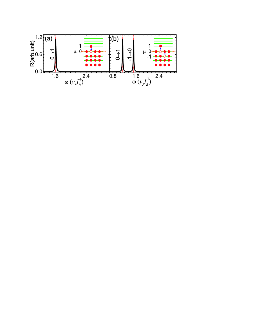
Figure 3: (Color online) The optical absorption curves with $\mu$=$0$ for (a) fully and (b) partially occupied cases. The spacer thickness is set to $d$=$0.2l_{B}$. The corresponding schematic sketch of magnetoexcitons are plotted in the insets.

The present general optical absorption selection rule proves to be very useful when analyzing magnetoexciton’s absorption resonant peaks in spectroscopy of TIB systems.

For simplicity, let us first consider the fully occupied case with $\mu$=$0$, i.e., electron LLs $n_{+}$$>$$0$ are unoccupied and hole LLs $n_{-}\mathtt{\leqslant}0$ are fully occupied. The ground state is $|0\rangle$=$|0,0\rangle$. According to the selection rule (17), the non-zero elements of $\langle n_{+},n_{-}|m_{x}^{-}|0,0\rangle$ only occurs at $n_{+}$=$1$ while $n_{-}$=$0$. That means there is only one resonant peak to appear in the absorption spectrum, which corresponds to the energy of magnetoexciton state $|1,0\rangle$ (see Fig. 3(a)). For comparison, we also study the partially occupied case with $\mu$=$0$. According to the selection rule (15), $\langle n_{+},n_{-}|m_{x}^{-}|0,0\rangle\mathtt{\neq}0$ only when $n_{+}$=$1$, $n_{-}$=$0$ or $n_{+}$=$0$, $n_{-}$=$-1$. Thus in this case there are two resonant peaks occurring in the absorption spectrum as shown in (see Fig. 3(b)), which correspond to the energies of two magnetoexciton states $|1,0\rangle$ and $|0,-1\rangle$. By increasing $d$ (equally decreasing the CI), these two magnetoexciton levels $|1,0\rangle$ and $|0,-1\rangle$ turn to be degenerate, which results in the incorporation of these two resonant peaks to be a single one at $d\mathtt{\rightarrow}\infty$. Schematic sketch of the corresponding magnetoexciton state obeying the selection rule (17) are plotted in the insets of Fig. 3.

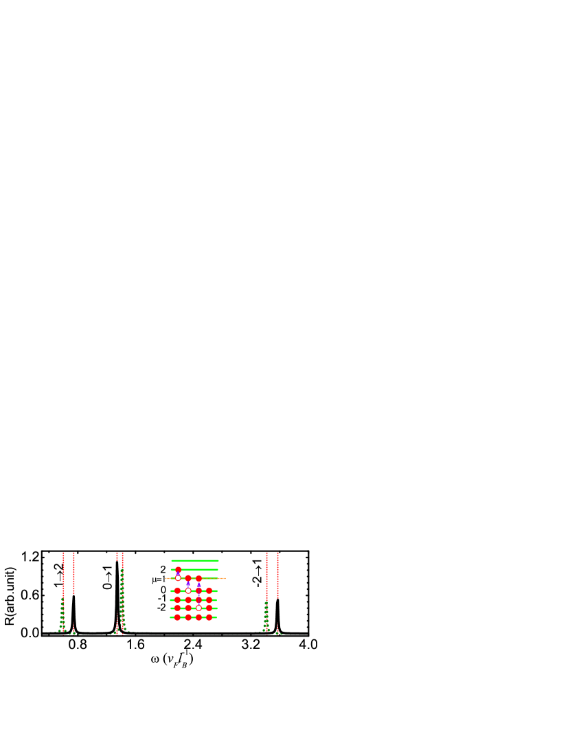
Figure 4: (Color online) Same as Fig. 3(b) except $\mu$=$1$. The green dotted curve represents the corresponding optical absorption spectrum at the limit of $d\mathtt{\rightarrow}\infty$.

To ulteriorly see the difference of absorption properties between partially and fully occupied cases, let us now consider the case of $\mu$=$1$, i.e., the ground state is $|1,1\rangle$. The selection rule for fully occupied case (Eq.(17)) with $\mu$=$1$ promises that there is only one resonant peak occurs, which corresponds to the formation of magnetoexciton state $|2,1\rangle$ by absorbing a photon quanta $\omega$. In the limit $d\mathtt{\rightarrow}\infty,$ $\omega\mathtt{\rightarrow}\sqrt{2}(\sqrt{2}\mathtt{-}1)$=$0.59$. For partially occupied case, however, there are three non-zero elements according to selection rule (15), which respectively are $n_{+}$=$1$, $n_{-}$=$0$; $n_{+}$=$1$, $n_{-}$=$-2$; and $n_{+}$=$2$, $n_{-}$=$1$. So there are three resonant peaks appearing in optical absorption spectrum (see black curves in Fig. 4 for $d$=$0.2l_{B}$), which correspond to the formation of magnetoexciton states $|2,1\rangle$, $|1,0\rangle$, and $|1,-2\rangle$, respectively, by absorbing photons of three different frequencies. As increasing the spacer thickness, these three absorption frequencies $\omega_{1}\mathtt{\rightarrow}\sqrt{2}(\sqrt{1}\mathtt{-}0)$=$1.41$, $\omega_{2}\mathtt{\rightarrow}\sqrt{2}(1\mathtt{+}\sqrt{2})$=$3.41$, and $\omega_{3}\mathtt{\rightarrow}\sqrt{2}(\sqrt{2}\mathtt{-}1)$=$0.59$ (see green dotted curves in Fig. 4).

When the interlevel CI is also included, the above-discussed magnetoexciton states will be mixed and energetically redistributed, which observably correct the exact selection rule (15) and bring about additional subsidiary peaks in the optical absorption spectrum. To clearly see this, we reconsider the case of $\mu$=$1$ as an example. The corresponding calculated optical absorption spectra for fully and partially occupied cases are respectively shown in Fig. 5(a) and 5(b).

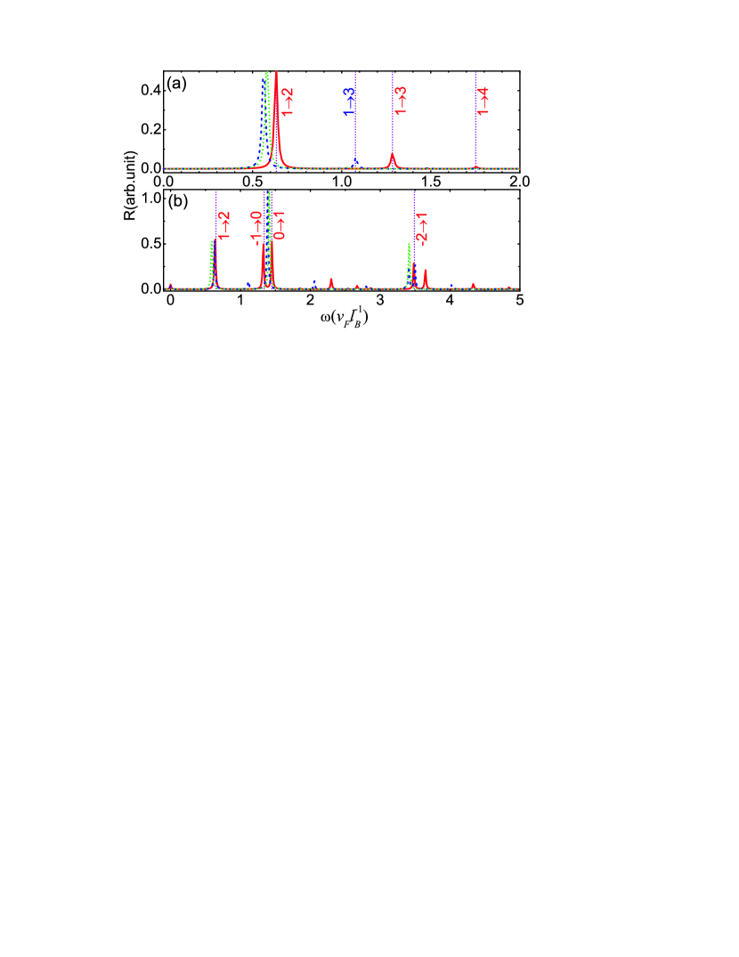
Figure 5: (Color online) The optical absorption spectrums with $\mu$=$1$ for (a) fully and (b) partially occupied cases when the interlevel Coulomb interaction is included. The red, blue and green curves are for $d$=$0.2l_{B}$, $2.0l_{B}$, and $10.0l_{B}$, respectively.

Let us first make an analysis on the fully occupied case. Because the interlevel CI mixes the noninteracting LLs, the absorption phenomenon should appear at the energy of every magnetoexciton state, with the resultant absorption peak amplitude decided by the projection of the corresponding resonant excited states $|n_{+},n_{-}\rangle$ allowed by the selection rule (15) in the case without interlevel interaction. When the spacer thickness $d$ is small (e.g. $d$=$0.2l_{B}$), not only the main resonant peak appears at the energy of excited level $|2,1\rangle$, but also two weak resonant peaks at the energies of excited levels $|3,1\rangle$ and $|4,1\rangle$ can be observed (see red curves in Fig. 5(a)). By increasing $d$ to $2.0l_{B}$, the resonant peak at $|3,1\rangle$ become faint and that at $|4,1\rangle$ disappears (blue dashed curves in Fig. 5(a)). When further increasing $d$ to $10.0l_{B}$, we find that the resonant peak $|3,1\rangle$ also disappears (green dotted curves in Fig. 5(a)) and the optical absorption spectrum comes back to the noninteracting case.

Similar physics also happens for partially occupied case (see Fig. 5(b)). The overlap caused by the interlevel CI between magnetoexciton states will produce many subsidiary resonant peaks besides the main peaks at the energies of magnetoexciton states $|2,1\rangle$, $|1,0\rangle$ and $|1,-2\rangle$. Note that there is a subsidiary resonant peak appearing in front of $|2,1\rangle$, which corresponds to the ground state $|1,1\rangle$. This special feature only appears for the partially occupied case and thus can be used to experimentally determine whether the highest occupied LL is fully filled or not in TIB. By increasing $d$, the subsidiary resonant peaks turn to disappear, and the optical absorption spectrum turns back to the noninteracting case: only the main three resonant peaks at energies of states $|2,1\rangle$, $|1,0\rangle$ and $|1,-2\rangle$ appear in absorption spectrum allowed by the selection rule (15).

In summary, we have theoretically studied the optical absorption properties of magnetoexcitons formed in TIB under a strong perpendicular magnetic field. By neglecting inter-Landau-level CI, we have determined an exact absorption selection rule, which greatly helps to connect absorption peaks with specific magnetoexcitons. The inclusion of inter-Landau-level CI has been shown to bring about subsidiary optical absorption peaks due to the mixing effect. Our present conclusion also works for graphene bilayers.

This work was supported by NSFC under Grants No. 10904005 and No. 90921003, and by the National Basic Research Program of China (973 Program) under Grant No. 2009CB929103.

References

- (1) D.W. Snoke, Science 298, 1368 (2002).
- (2) L.V. Butov, J. Phys.: Condens. Matter 16, R1577 (2004).
- (3) V.B. Timofeev and A.V. Gorbunov, J. Appl. Phys. 101, 081708 (2007).
- (4) J.P. Eisenstein and A.H. MacDonald, Nature (London) 432, 691 (2004).
- (5) C.H. Zhang and Y.N. Joglekar, Phys. Rev. B 77, 233405 (2008).
- (6) H. Min, R. Bistritzer, J.-J. Su, and A. H. MacDonald, Phys. Rev. B 78, 121401(R) (2008).
- (7) Yu. E. Lozovik and A. A. Sokolik, Pis’ma v ZhETF, 87, 61 (2008). [JETP Lett. 87, 55 (2008)].
- (8) A. Iyengar, J.H. Wang, H.A. Fertig, and L. Brey, Phys. Rev. B 75, 125430 (2007).
- (9) O.L. Berman, Y.E. Lozovik, and G. Gumbs, Phys. Rev. B 77, 155433 (2008).
- (10) O.L. Berman, R.Ya. Kezerashvili, and Y.E. Lozovik, Phys. Rev. B 78, 035135 (2008).
- (11) Z.G. Koinov, Phys. Rev. B 79, 073409 (2009).
- (12) C.L. Kane and E.J. Mele, Phys. Rev. Lett. 95, 226801 (2005); 95, 146802 (2005).
- (13) B.A. Bernevig and S.C. Zhang, Phys. Rev. Lett. 96, 106802 (2006).
- (14) L. Fu and C. L. Kane, Phys. Rev. B 76, 045302 (2007).
- (15) M. König, S. Wiedmann, Christoph Brüne, A. Roth, H. Buhmann, L. W. Molenkamp, X.-L. Qi, and S. C. Zhang, Science 318, 766 (2007).
- (16) D. Hsieh, D. Qian, L. Wray, Y. Xia, Y. S. Hor, R. J. Cava, and M. Z. Hasan, Nature 452, 970 (2008).
- (17) J.E. Moore, Nature (London) 464, 194 (2010).
- (18) X.-L. Qi and S.-C. Zhang, Phys. Today 63, 33 (2010).
- (19) M.Z. Hasan and C.L. Kane, Rev. Mod. Phys. 82, 3045 (2010), and references therein.
- (20) X.L. Qi and S.C. Zhang, Rev. Mod. Phys. 83, 1057 (2011), and references therein.
- (21) H.-J. Zhang, C.-X. Liu, X.-L. Qi, X. Dai, Z. Fang, and S.-C. Zhang, Nature Phys. 5, 438 (2009).
- (22) Y. Xia, D. Qian, D. Hsieh, L. Wrayl, A. Pal1, H. Lin, A. Bansil, D. Grauer, Y. S. Hor, R. J. Cava, Nat. Phys. 5, 398 (2009).
- (23) Y. L. Chen, J. G. Analytis, J. H. Chu, Z. K. Liu, S. K. Mo, X. L. Qi, H. J. Zhang, D. H. Lu, X. Dai, Z. Fang, Science 325, 178 (2009).
- (24) C.-Z. Chang, K. He, L.-L. Wang, X.-C. Ma, M.-H. Liu, Z.-C. Zhang, X. Chen, Y.-Y. Wang, and Q.-K. Xue, Spin 1, 21 (2011).
- (25) Z. Li, Y. Qin, Y. Mu, T. Chen, C. Xu, L. He, J. Wan, F. Song, M. Han, G. Wang, J. Nanosci. Nanotechnol. 11, 7042 (2011).
- (26) H. Liu and P.D. Ye, Appl. Phys. Lett. 99, 052108 (2011).
- (27) R. Valdés Aguilar, A. V. Stier, W. Liu, L.S. Bilbro, D. K. George, N. Bansal, L. Wu, J. Cerne, A. G. Markelz, S. Oh, and N.P. Armitage, Phys. Rev. Lett. 108, 087403 (2012).
- (28) M. V. Marquezini, M. J. S. P. Brasil, M. A. Cotta, and J. A. Brum, Phys. Rev. B 53, R16156 (1996).
- (29) Y. Kim, K.-S. Lee, and C. H. Perry, Appl. Phys. Lett. 84, 738 (2004).
- (30) A. D. LaForge, A. Frenzel, B. C. Pursley, T. Lin, X. Liu, J. Shi, and D. N. Basov, Phys. Rev. B 81, 125120 (2010).
- (31) C.-X. Liu, X.-L. Qi, H. Zhang, X. Dai, Z. Fang, and S.-C. Zhang, Phys. Rev. B 82, 045122 (2010).
- (32) Z. Wang, Z.-G. Fu, S.-X. Wang, and P. Zhang, Phys. Rev. B 82, 085429 (2010).