Transport of angular momentum and chemical species by anisotropic mixing in stellar radiative interiors

Abstract

Small levels of turbulence can be present in stellar radiative interiors due to, e.g., instability of rotational shear. In this paper we estimate turbulent transport coefficients for stably stratified rotating stellar radiation zones. Stable stratification induces strong anisotropy with a very small ratio of radial-to-horizontal turbulence intensities. Angular momentum is transported mainly due to the correlation between azimuthal and radial turbulent motions induced by the Coriolis force. This non-diffusive transport known as the $\Lambda$-effect has outward direction in radius and is much more efficient compared to the effect of radial eddy viscosity. Chemical species are transported by small radial diffusion only. This result is confirmed using direct numerical simulations combined with the test-scalar method. As a consequence of the non-diffusive transport of angular momentum, the estimated characteristic time of rotational coupling ($\;\buildrel<\over{\scriptstyle\sim}\;$100 Myr) between radiative core and convective envelope in young solar-type stars is much shorter compared to the time-scale of Lithium depletion ($\sim 1$ Gyr).

1 Introduction

Mixing of material in stably stratified stellar radiative interiors is opposed by buoyancy forces. Nevertheless, a certain level of turbulence resulting, e.g., from instabilities of rotational shear (Goldreich & Schubert [1967]) or forcing from the upper convection zone (Blöcker et al. [1998]) is possible and even necessary to explain rotational coupling between the radiative core and the convective envelope, and thus the depletion of light elements in solar-type stars.

Turbulent transport in stellar radiation zones is supposed to be strongly anisotropic (Spiegel & Zahn [1992]; Denissenkov [2010]). Buoyancy forces suppress radial mixing so that much higher horizontal compared with radial velocities might be expected. The degree of the anisotropy is not certain, however. It remains a free parameter of transport models. The anisotropy in rotating fluids is, however, not free (Rüdiger & Pipin [2001]). The influence of the Coriolis force on horizontal motions produces radial displacements. The ratio of radial to azimuthal mixing intensities is controlled by the balance between Coriolis and buoyancy forces.

The aim of this paper is to estimate the effects of rotation and stable stratification on turbulence. We do not specify here the origin of the turbulence but just prescribe the so-called ‘original turbulence’ that would take place in non-rotating and neutrally stratified fluid. The combined effect of rotation and stable stratification on this original turbulence is then estimated.

We shall see that the resulting parameters of turbulent mixing depend only slightly on the properties of the prescribed original turbulence. In particular, the anisotropy,

$$\frac{\langle u_{\phi}^{2}\rangle}{\langle u_{r}^{2}\rangle}\approx\frac{\tau^{2}N^{4}}{\Omega^{2}},$$ (1)

varies only slightly between very different prescriptions (in this equation, $u$ is the fluctuating velocity, $\Omega$ is the angular velocity, $N$ is the buoyancy frequency, and $\tau$ is the eddy turnover time). Typically, $\Omega\ll N$ in radiation zones and probably we also have $\tau N\gg 1$. Therefore, the anisotropy of Eq. (1) is high. Our main finding is that the strongly anisotropic turbulence is much more efficient in transporting angular momentum than chemical species. The reason is that the Coriolis force makes the azimuthal and radial motions correlated. Fluid particles with positive (negative) azimuthal velocity are pushed by the Coriolis force in the positive (negative) radial direction. As a result, $\langle u_{r}u_{\phi}\rangle>0$, and the turbulence transports angular momentum in the positive radial direction. This angular momentum flux cannot be interpreted as an effect of eddy viscosity, i.e., it is not diffusive by nature. Transport of chemical species, on the contrary, is only due to radial turbulent mixing.

The non-diffusive transport of angular momentum that we find is essentially the well-known $\Lambda$-effect of differential rotation theory (Lebedinskii [1941]; Rüdiger [1989]). The effect has been well studied for nearly adiabatically stratified stellar convection zones. Our paper suggests that it can be important for the rotational coupling between radiative interiors and convective envelopes as well.

2 Mathematical formulation

2.1 Relation between the original and background turbulence

To specify the effects of rotation and stable stratification on turbulence, we follow the standard approach of quasilinear theory by formulating the linear relation, $u_{i}=D_{ij}u^{(0)}_{j}$ between the velocity fields of original turbulence ${\mbox{\boldmath$u$}}^{(0)}$, which would take place in nonrotating neutrally stratified fluid, and actual or background turbulence $u$. The relation tensor $D_{ij}$ includes the effects of rotation and stratification.

We apply a simple version of the $\tau$-approximation to write the equations for fluctuating velocity and entropy as follows,

$$\frac{\mbox{\boldmath$u$}}{\tau} + 2{\mbox{\boldmath$\Omega$}}\times{\mbox{\boldmath$u$}}+\frac{1}{\rho}{\mbox{\boldmath$\nabla$}}P-\mbox{\boldmath$g$}={\mbox{\boldmath$f$}},$$

$$\frac{s^{\prime}}{\tau} = -({\mbox{\boldmath$u$}}\cdot{\mbox{\boldmath$\nabla$}})\langle s\rangle,$$ (2)

where $f$ is a random force driving the turbulence, $\tau$ is the eddy turnover time, $g$ is gravity and the $\tau$-relaxation terms replace the nonlinear terms together with time-derivatives,

$$\frac{\partial\mbox{\boldmath$u$}}{\partial t}+({\mbox{\boldmath$u$}}\cdot{\mbox{\boldmath$\nabla$}}){\mbox{\boldmath$u$}}-\langle({\mbox{\boldmath$u$}}\cdot{\mbox{\boldmath$\nabla$}}){\mbox{\boldmath$u$}}\rangle\rightarrow\frac{\mbox{\boldmath$u$}}{\tau},$$

$$\frac{\partial s^{\prime}}{\partial t}+{\mbox{\boldmath$u$}}\cdot{\mbox{\boldmath$\nabla$}}s-\langle{\mbox{\boldmath$u$}}\cdot{\mbox{\boldmath$\nabla$}}s\rangle\rightarrow\frac{s^{\prime}}{\tau}.$$ (3)

Microscopic diffusion is neglected. The $\tau$-approximation (3) assumes that the nonlinear interaction of turbulent eddies leads to their effective dissipation (a turbulent fragmentation of scales) in a characteristic time $\tau\approx\ell/u$, where $\ell$ is the characteristic spatial scale of the eddies. We assume that the motion is incompressible, $\mathrm{div}{\mbox{\boldmath$u$}}=0$. This means that vertical displacements are small compared to the density scale height and velocities are small compared to the speed of sound.

Fourier transformation is applied,

$${\mbox{\boldmath$u$}}({\mbox{\boldmath$r$}}) = \int\mathrm{e}^{\mathrm{i}{\bm{k}}\cdot{\bm{r}}}\tilde{\mbox{\boldmath$u$}}({\mbox{\boldmath$k$}})\ \mathrm{d}{\mbox{\boldmath$k$}},$$

$$s^{\prime}({\mbox{\boldmath$r$}}) = \int\mathrm{e}^{\mathrm{i}{\bm{k}}\cdot{\bm{r}}}\tilde{s}^{\prime}({\mbox{\boldmath$k$}})\ \mathrm{d}{\mbox{\boldmath$k$}},$$ (4)

to convert the partial differential equations (2) into algebraic equations. We neglect variations of mean fields on the spatial scale of the turbulence to obtain a closed equation for the fluctuating velocity:

$$\tilde{u}_{i}+{N^{*}}^{2}(\hat{r}_{i}-\mu\hat{k}_{i})(\hat{\mbox{\boldmath$r$}}\cdot\tilde{\mbox{\boldmath$u$}})+\sigma\Omega^{*}\varepsilon_{ipm}\hat{k}_{p}\tilde{u}_{m}=\tilde{u}^{(0)}_{i}$$ (5)

(cf. Kitchatinov & Rüdiger ([2008]) on how the pressure term is treated). In Eq. (5), $\hat{\mbox{\boldmath$r$}}$ is the radial unit vector, $\hat{\mbox{\boldmath$k$}}={\mbox{\boldmath$k$}}/k$ is the unit vector along the wave vector, $\mu=(\hat{\mbox{\boldmath$k$}}\cdot\hat{\mbox{\boldmath$r$}})$ is the cosine of the angle between wave vector and radius, and $\sigma=(\hat{\mbox{\boldmath$k$}}\cdot{\mbox{\boldmath$\Omega$}})/\Omega$ is cosine of the angle between the wave vector and rotation axis. The Coriolis number

$$\Omega^{*}=2\tau\Omega$$ (6)

and the normalized buoyancy frequency

$$N^{*}=\tau N,\ \ \ \ \ \ N^{2}=\frac{g}{c_{\mathrm{p}}}\frac{\partial\langle s\rangle}{\partial r},$$ (7)

parameterize the effects of rotation and stratification.

Solving Eq. (5) for $\tilde{\mbox{\boldmath$u$}}$ gives the relation tensor,

$$D_{ij} = \frac{1}{1+{N^{*}}^{2}(1-\mu^{2})+\sigma^{2}{\Omega^{*}}^{2}}\times$$

$$\bigg{(}\left(1+{N^{*}}^{2}(1-\mu^{2})\right)\left(\delta_{ij}+\sigma\Omega^{*}\varepsilon_{ijp}\hat{k}_{p}\right)-$$

$$-\ {N^{*}}^{2}(\hat{r}_{i}-\mu\hat{k}_{i})\hat{r}_{j}+$$

$$+\ \sigma\Omega^{*}{N^{*}}^{2}\left((\hat{r}_{i}-\mu\hat{k}_{i})\varepsilon_{jmp}-\hat{r}_{j}\varepsilon_{imp}\right)\hat{r}_{m}\hat{k}_{p}\bigg{)},$$

$$\tilde{u}_{i} = D_{ij}\tilde{u}_{j}^{(0)}.$$ (8)

This equation describes the joint influence of rotation and stable stratification on the turbulence.

In the limit of neutral stratification, $N^{*}\rightarrow 0$, Eq. (8) reduces to the familiar expression (Kitchatinov [1986])

$$D_{ij}=\frac{\delta_{ij}+\sigma\Omega^{*}\varepsilon_{ijp}\hat{k}_{p}}{1+\sigma^{2}{\Omega^{*}}^{2}},$$ (9)

describing the influence of rotation in the $\tau$-approximation. In the other limit of slow rotation, $\Omega^{*}\rightarrow 0$, Eq. (8) reduces to

$$D_{ij}=\delta_{ij}-\frac{{N^{*}}^{2}}{1+{N^{*}}^{2}(1-\mu^{2})}(\hat{r}_{i}-\mu\hat{k}_{i})\hat{r}_{j}.$$ (10)

This equation accounts for the effect of stable stratification alone.

2.2 Original turbulence models

The original turbulence properties can be prescribed by specifying the spectral tensor $\tilde{Q}^{(0)}_{ij}$:

$$\langle\tilde{u}^{(0)}_{i}({\mbox{\boldmath$k$}})\tilde{u}^{(0)}_{j}({\mbox{\boldmath$k$}}^{\prime})\rangle=\tilde{Q}^{(0)}_{ij}({\mbox{\boldmath$k$}})\ \delta({\mbox{\boldmath$k$}}+{\mbox{\boldmath$k$}}^{\prime})$$ (11)

(Rüdiger [1989]). The relation tensor (8) can then be used to account for the effects of rotation and stratification,

$$\tilde{Q}_{ij} = D_{im}D_{jn}\tilde{Q}^{(0)}_{mn},$$

$$Q_{ij} = \langle u_{i}u_{j}\rangle=\int\tilde{Q}_{ij}({\mbox{\boldmath$k$}})\ \mathrm{d}{\mbox{\boldmath$k$}}.$$ (12)

For the simplest case of isotropic nonhelical turbulence the spectral tensor reads

$$\tilde{Q}_{ij}^{(0)}=\frac{E(k)}{8\pi k^{2}}\left(\delta_{ij}-\hat{k}_{i}\hat{k}_{j}\right).$$ (13)

In this equation, $E$ is the spectrum function

$$\langle u^{2}\rangle^{(0)}=\int\limits_{0}^{\infty}E(k)\mathrm{d}k.$$ (14)

A more realistic model is anisotropic turbulence with a preferred direction being the radial one. Horizontal velocities are expected to be much larger than the vertical ones. For the extreme case of strictly horizontal random motions, we have

$$\tilde{Q}_{ij}^{(0)}=q(k,\mu)\times\ \ \ \ \ \ \ \ \ \ \ \$$

$$\big{(}(1-\mu^{2})(\delta_{ij}-\hat{k}_{i}\hat{k}_{j}) - (\hat{r}_{i}-\mu\hat{k}_{i})(\hat{r}_{j}-\mu\hat{k}_{j})\big{)}.$$ (15)

The correlation lengths for vertical and horizontal directions may differ. If, however, the lengths are equal, the $q$-function in Eq. (15) does not depend on $\mu$:

$$q=\frac{3E(k)}{8\pi k^{2}}.$$ (16)

The case where the correlation length in radius is small compared to the horizontal correlation length can be modeled by the equation

$$q=\frac{3E(k_{\perp})\ k_{\perp}}{8\pi k^{3}},\ \ \ \ \ \ k_{\perp}=k\sqrt{1-\mu^{2}}.$$ (17)

The spectrum functions $E$ of Eqs. (16) and (17) are related to the turbulence intensity by the same equation (14) as in the case of the isotropic turbulence of Eq. (13).

Anisotropic turbulence that has finite radial velocities (but different from the horizontal velocities) can be modeled by a linear superpositions of the spectral tensors (13) and (15). We shall see that, if the buoyancy frequency is large compared to the rotation frequency, $N\gg\Omega$, and the normalized buoyancy frequency is large, $N^{*}\gg 1$, which are conditions typical of stellar radiation zones, then the turbulent transport parameters differ little between the representations (13), (16) and (17) for the original turbulence, i.e., the transport characteristics are not sensitive to a particular choice of the original turbulence model.

2.3 Direct numerical simulations

An independent verification of the effects of strong stratification on turbulent diffusion is provided by means of direct numerical simulations. In that case, we solve the full set of compressible hydrodynamic equations for $\rho$, $\bm{u}$, and $s$:

$$\frac{{\rm D}\rho}{{\rm D}t} \!=\! -\rho\bm{\nabla}\cdot\bm{u},$$ (18)

$$\rho\frac{{\rm D}\bm{u}}{{\rm D}t} \!=\! -\bm{\nabla}P+\bm{\nabla}\cdot(2\rho\nu\bm{\mathsf{S}})+\rho({\bm{f}}+{\bm{g}}),$$ (19)

$$\rho T\frac{{\rm D}s}{{\rm D}t} \!=\! \bm{\nabla}\cdot K\bm{\nabla}T+2\rho\nu\bm{\mathsf{S}}^{2}-\frac{1}{\tau_{s}}\rho(c_{\rm s}^{2}-c_{\rm s0}^{2}),$$ (20)

where ${\rm D}/{\rm D}t=\partial/\partial t+\bm{u}\cdot\bm{\nabla}$ is the advective derivative, ${\sf S}_{ij}=\textstyle{\frac{1}{2}}(u_{i,j}+u_{j,i})-\textstyle{\frac{1}{3}}\delta_{ij}\bm{\nabla}\cdot\bm{u}$ is the traceless rate of strain tensor, commas indicate partial differentiation, $\nu$ is the kinematic viscosity, the specific entropy is given by $s=c_{\rm v}\ln P-c_{\rm v}\ln\rho$, where $c_{\rm p}$ and $c_{\rm v}$ are the specific heats at constant pressure and constant volume, respectively, the temperature is related to $P$ and $\rho$ via $(c_{\rm p}-c_{\rm v})T=P/\rho$, which, in turn, is related to the sound speed $c_{\rm s}$ via $c_{\rm s}^{2}=\gamma P/\rho$, where $\gamma=c_{\rm p}/c_{\rm v}$ is the ratio of specific heats, ${\bm{f}}$ is the external forcing function, and $K$ is the thermal conductivity. The last term in the entropy equation (20) represents a cooling term that keeps the temperature (or sound speed) approximately constant with a given relaxation or cooling time $\tau_{s}$. The flow is driven by a random forcing function consisting of nonhelical waves with wavenumbers whose modulus lie in a narrow band around an average wavenumber $k_{\rm f}$ (Haugen et al. [2004]). We arrange the amplitude of the forcing function such that the Mach number based on the rms velocity remains below 0.1, so the effects of compressibility are negligible.

We consider a cubic domain of size $L^{3}$ with periodic boundary conditions in the $x$ and $y$ directions and insulating impenetrable stress-free boundary conditions on $z=\pm L/2$. The mass in the volume is therefore conserved and given by $\int\rho\,{\rm d}^{3}x=\rho_{0}L^{3}$. The lowest wavenumber that fits into the domain is $k_{1}=2\pi/L$. Our average forcing $k_{\rm f}$ wavenumber is chosen such that $k_{\rm f}/k_{1}=5$. We adopt isothermal initial conditions with $c_{\rm s}=c_{\rm s0}$ and $\rho=\rho_{0}\exp(-z/H)$, where $H=c_{\rm s0}^{2}/\gamma g$ is the scale height which is chosen such that $Hk_{1}=1$. The turnover time based on the wavenumber $k_{\rm f}$ is $\tau=(u_{\rm rms}k_{\rm f})^{-1}$, where $u_{\rm rms}$ is the rms velocity based on all three velocity components. We vary the normalized buoyancy frequency by varying the forcing amplitude. For each run the viscosity is adjusted such that the Reynolds number, $\mbox{Re}=u_{\rm rms}/\nu k_{\rm f}$, is around 40. The Prandtl number, $\mbox{Pr}=\nu c_{\rm p}\rho/K$, is chosen to be equal to unity. The cooling time is chosen such that $\tau_{s}u_{\rm rms}k_{\rm f}$ is also around unity.

To quantify the suppression of vertical mixing in a numerical simulation of stratified turbulence we use the test-scalar method by solving equations for the fluctuating passive scalar concentration in the presence of a prescribed mean passive scalar concentration,

$${\partial c^{pq}\over\partial t}=-\bm{\nabla}\cdot(\bm{u}C^{pq}+\bm{u}c^{pq}-\langle\bm{u}c^{pq}\rangle)+\kappa\nabla^{2}c^{pq},$$ (21)

where $\bm{u}$ is the velocity fluctuation obtained from Eq. (19), and the mean flow is zero. The superscript $p$ (=1 or 3) stands for test scalars varying in the $x$ or $z$ directions while $q$ stands for c and s that represent mean fields that are proportional to $\cos kx_{p}$ or $\sin kx_{p}$, respectively,

$$C^{pc}=C_{0}\cos kx_{p},\quad C^{ps}=C_{0}\sin kx_{p},\\$$ (22)

where $(x_{1},x_{2},x_{3})=(x,y,z)$ are Cartesian coordinates and $C_{0}$ is a normalization factor. Angle brackets denote planar averaging over the $yz$ plane (if $p=1$) or the $xy$ plane (if $p=3$). The passive scalar flux is then related to the gradient of $C^{pc}$ via $\langle u_{i}c^{pq}\rangle=-\kappa_{ij}\nabla_{j}C^{pc}$, where $\kappa_{ij}$ are the components of the turbulent diffusivity tensor, obtained as

$$\kappa_{xx} \!=\! (\sin kx\langle u_{x}c^{1c}\rangle-\cos kx\langle u_{x}c^{1s}\rangle)/kC_{0},$$ (23)

$$\kappa_{zz} \!=\! (\sin kz\langle u_{z}c^{1c}\rangle-\cos kz\langle u_{z}c^{1s}\rangle)/kC_{0},$$ (24)

by using the solutions for four different test scalars. These coefficients depend on time and one spatial coordinate, but because of stationarity and approximate homogeneity of the turbulence intensity, we present in the following temporal and spatial averages of these coefficients.

The test scalar method has been used previously to quantify mixing in turbulence in the presence of rotation and magnetic fields (Brandenburg et al. [2009]), shear (Madarassy & Brandenburg [2010]), as well as isothermal density stratification (Brandenburg et al. [2012]). However, unlike those earlier works, the entropy equation is here included and a non-isothermal equation of state for a perfect monatomic gas is used with $\gamma=5/3$. Equations (18)–(21) are solved using the Pencil Code in three dimensions. The numerical resolution used for the simulations presented here is $128^{3}$ meshpoints. Like the Prandtl, the Schmidt number, $\mbox{Sc}=\nu/\kappa$, is also chosen to be equal to unity.

3 The effect of stable stratification

We consider first the effect of stable stratification for a non-rotating fluid, $\Omega=0$. The only preferred direction in this case is the radial one. For any model of the original turbulence, we therefore have

$$\langle u_{i}u_{j}\rangle=\frac{\langle u^{2}_{\mathrm{h}}\rangle}{2}\left(\delta_{ij}-\hat{r}_{i}\hat{r}_{j}\right)+\langle u^{2}_{r}\rangle\hat{r}_{i}\hat{r}_{j},$$ (25)

where $\langle u^{2}_{\mathrm{h}}\rangle=\langle u^{2}_{\phi}\rangle+\langle u^{2}_{\theta}\rangle$ is the horizontal turbulence intensity. Standard spherical coordinates ($r,\theta,\phi$) are used.

On using the relation tensor (10) and Eq. (12) for the isotropic original turbulence of Eq. (13), we find

$$\langle u^{2}_{\mathrm{h}}\rangle=\langle u^{2}\rangle^{(0)}\bigg{(}\frac{1}{2}+\frac{1}{4{N^{*}}^{2}}-$$

$$\left.-\frac{1}{8{N^{*}}^{3}\sqrt{{N^{*}}^{2}+1}}\ \mathrm{ln}\left(\frac{\sqrt{{N^{*}}^{2}+1}+N^{*}}{\sqrt{{N^{*}}^{2}+1}-N^{*}}\right)\right),$$ (26)

$$\langle u^{2}_{r}\rangle=\frac{\langle u^{2}\rangle^{(0)}}{4{N^{*}}^{2}({N^{*}}^{2}+1)}\times$$

$$\left(\frac{2{N^{*}}^{2}+1}{2N^{*}\sqrt{{N^{*}}^{2}+1}}\ \mathrm{ln}\left(\frac{\sqrt{{N^{*}}^{2}+1}+N^{*}}{\sqrt{{N^{*}}^{2}+1}-N^{*}}\right)-1\right).$$ (27)

Figure 1 shows the ratio of vertical to horizontal turbulence intensities as a function of the normalized buoyancy frequency $N^{*}$. Squares on the plot show the results of direct numerical simulations described in Sect. 2.3.

Figure 1: Ratio of the vertical to horizontal turbulence intensities in dependence on the normalized buoyancy frequency (7) for the case of a non-rotating fluid and isotropic original turbulence. Squares show the results of 3D direct numerical simulations for isotropically forced turbulence.

Horizontal turbulence intensity is influenced by the stable stratification only slightly. In the limit of very large $N^{*}$, it is $\langle u^{2}_{\mathrm{h}}\rangle=\langle u^{2}\rangle^{(0)}/2$, i.e., $\langle u^{2}_{\mathrm{h}}\rangle$ is reduced compared to the case of a non-stratified fluid by a factor of 3/4 only. The vertical motions, by contrast, are strongly suppressed:

$$\langle u^{2}_{r}\rangle\simeq\frac{\langle u^{2}\rangle^{(0)}}{4{N^{*}}^{4}}\left(\mathrm{ln}(4{N^{*}}^{2})-1\right)\ \ \ \mathrm{for}\ \ N^{*}\gg 1$$ (28)

in the strong stratification limit. The originally isotropic turbulence is changed towards horizontal turbulence as $N^{*}$ increases.

As might be expected, the horizontal turbulence of Eq. (15) is not influenced by the stratification at all, i.e., $Q_{ij}=Q^{(0)}_{ij}$ in this case. Therefore, whatever model for the original turbulence in Section 2.2 is used, the resulting turbulence in the limit of large $N^{*}$ is almost the same. The only difference between isotropic and horizontal original turbulence models is that for the first case the radial velocities of Eq. (28) are finite, although very small.

Figure 2: Dependence of $\kappa_{xx}/\kappa_{\rm t0}$ (open symbols) and $\kappa_{zz}/\kappa_{\rm t0}$ (filled symbols) on the normalized buoyancy frequency. The dashed line shows that $\kappa_{xx}/\kappa_{\rm t0}\approx 2.5$ while the solid line gives $\kappa_{zz}/\kappa_{\rm t0}\approx 0.09\,(\tau N)^{-3/2}$.

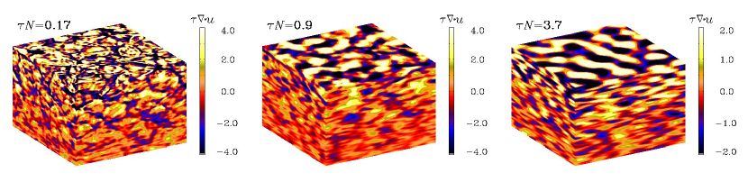
Figure 3: Visualizations of $\tau\bm{\nabla}\cdot\bm{u}$ on the periphery of the computational domain for $\tau N=0.17$, 0.9, and 3.7.

Similar results are obtained numerically for the turbulent diffusivity using the test-scalar method; see Fig. 2, where we plot $\kappa_{xx}$ and $\kappa_{zz}$, both normalized by the reference value $\kappa_{\rm t0}=u_{\rm rms}/3k_{\rm f}$. Note that $\kappa_{xx}/\kappa_{\rm t0}\approx 2.5$, independent of $\tau N$, while $\kappa_{zz}/\kappa_{\rm t0}\approx 0.09\,(\tau N)^{-3/2}$. Visualizations of the scalar quantity $\tau\bm{\nabla}\cdot\bm{u}$ on the periphery of the computational domain (Fig. 3) confirm our expectation that turbulent structures that become flatter as $\tau N$ is increased. These structures become smoother in the $xy$ plane, while their length scale in the $z$ direction decreases.

4 Mixing in rotating and stratified fluids

Similarity of the results for different original turbulence models is even more pronounced when rotation is included. Coriolis force produces radial motion even for original horizontal turbulence. The relative intensity of radial mixing is controlled by the balance between buoyancy and Coriolis forces.

Producing analytical results for arbitrary values of $N^{*}$ and $\Omega^{*}$ is problematic. Derivations were performed for the practically interesting case of strong stratification, $N^{*}\gg 1$, and not too fast rotation, $\Omega^{*}\ll N^{*}$. The period of gravity waves for radiation zones of solar-type stars is of the order of one hour. The characteristic time of turbulence is probably much longer (it is about one month for convection and probably longer for radiation zone motions), so that the condition $N^{*}\gg 1$ is well satisfied. The condition $\Omega^{*}\ll N^{*}$ should be satisfied as well in radiation zones of pressure supported stars (otherwise we are dealing with centrifugally supported disks).

We now use Eq. (8) for the relation tensor that includes the combined effects of rotation and stratification. For the case of the isotropic original turbulence of Eq. (13), the terms of lowest order in ${N^{*}}^{-1}$ in the most significant velocity correlations read

$$\langle u_{\mathrm{h}}^{2}\rangle = \frac{1}{2}\langle u^{2}\rangle^{(0)},$$

$$\langle u^{2}_{r}\rangle = \frac{\langle u^{2}\rangle^{(0)}}{4{N^{*}}^{4}}\left[\mathrm{ln}\left(\frac{4{N^{*}}^{2}}{1+{\Omega^{*}}^{2}\cos^{2}\theta}\right)-1+{\Omega^{*}}^{2}\right.$$

$$+ \left.{\Omega^{*}}^{2}\cos^{2}\theta\left(\mathrm{ln}\left(\frac{4{N^{*}}^{2}}{1+{\Omega^{*}}^{2}\cos^{2}\theta}\right)-4\right)\right],$$

$$\langle u_{r}u_{\theta}\rangle = \langle u^{2}\rangle^{(0)}\frac{{\Omega^{*}}^{2}}{4{N^{*}}^{4}}\left(\mathrm{ln}\left(\frac{4{N^{*}}^{2}}{1+{\Omega^{*}}^{2}\cos^{2}\theta}\right)-3\right)$$

$$\times\sin\theta\cos\theta,$$

$$\langle u_{r}u_{\phi}\rangle = \langle u^{2}\rangle^{(0)}\frac{\Omega^{*}}{4{N^{*}}^{2}}\sin\theta.$$ (29)

The turbulence intensities $\langle u^{2}_{\mathrm{h}}\rangle$ and $\langle u_{r}^{2}\rangle$ control the eddy diffusion in latitude and radius, respectively. The cross-correlation $\langle u_{r}u_{\phi}\rangle$ is important for transport of angular momentum. The correlation $\langle u_{r}u_{\theta}\rangle$ may cause the temperature variation with latitude; positive $\langle u_{r}u_{\theta}\rangle\cos\theta$ implies poleward eddy heat flux. It may be noted that rotation does not produce anisotropy in the horizontal plane in the strong stratification limit, $\langle u_{\theta}^{2}\rangle=\langle u_{\phi}^{2}\rangle=\langle u_{\mathrm{h}}^{2}\rangle/2$ (more precisely, the anisotropy is small: $(\langle u_{\theta}^{2}\rangle-\langle u_{\phi}^{2}\rangle)/\langle u_{\mathrm{h}}^{2}\rangle\sim{\Omega^{*}}^{2}/{N^{*}}^{4}$).

The results for horizontal turbulence of Eq. (15) with an isotropic correlation length of Eq. (16) or a short vertical correlation length of Eq. (17) are the same and read

$$\langle u_{\mathrm{h}}^{2}\rangle = \langle u^{2}\rangle^{(0)},$$

$$\langle u^{2}_{r}\rangle = \langle u^{2}\rangle^{(0)}\frac{{\Omega^{*}}^{2}}{2{N^{*}}^{4}},$$

$$\langle u_{r}u_{\theta}\rangle = \langle u^{2}\rangle^{(0)}\frac{{\Omega^{*}}^{2}}{2{N^{*}}^{4}}\sin\theta\cos\theta,$$

$$\langle u_{r}u_{\phi}\rangle = \langle u^{2}\rangle^{(0)}\frac{\Omega^{*}}{2{N^{*}}^{2}}\sin\theta.$$ (30)

If the Coriolis number (6) is not small ($\Omega^{*}>1$), equations (29) and (30), though different in details, are of the same order of magnitude. As the $\tau$-approximation, which was used to derive these equation, probably has the same accuracy, the results are practically the same. We focus in the following discussion on the results of Eq. (30) because the case of horizontal original turbulence is probably more adequate for stably stratified fluids.

5 Discussion

A remarkable feature of Eq. (30) is the finite cross-correlation $\langle u_{r}u_{\phi}\rangle$. This means that the turbulence transports angular momentum in radius. The cross-correlation is positive so that the angular momentum is transported outward. For the case of differential rotation caused by stellar spin-down, this angular momentum flux acts in same direction as turbulent viscosity, but it is not viscous by nature.

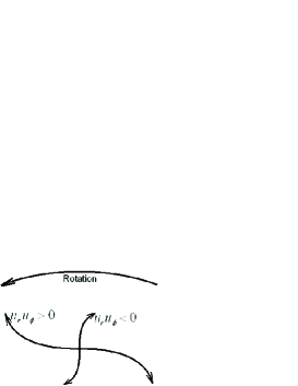
Figure 4: Illustration of the origin of non-viscous angular momentum transport by anisotropic turbulence (see text).

What we find here is the known $\Lambda$-effect of differential rotation theory (Lebedinskii [1941]; Rüdiger [1989]). Figure 4 illustrates its origin. The positive correlation $\langle u_{r}u_{\phi}\rangle$ results from the Coriolis force action on the original horizontal motion. The fluid particles, which move in the direction of global rotation, are deflected outwards in radius by the Coriolis force. Fluid particles moving in the retrograde direction are deflected inwards. The product $u_{r}u_{\phi}$ is positive in both cases. Note that the influence of the Coriolis force on the original radial motion produces a negative correlation $\langle u_{r}u_{\phi}\rangle<0$ (Fig. 4). The sense of radial angular momentum transport is controlled by the turbulence anisotropy. Angular momentum is transported inward if radial mixing prevails and outward for predominantly horizontal mixing (Rüdiger [1989]). In the present case, the anisotropy of horizontal type is produced by the stable stratification. It may be noticed that we do not find a meridional $\Lambda$-effect. The meridional flux of angular momentum is of higher order in ${N^{*}}^{-2}$ compared to the radial flux. This is a consequence of small anisotropy in the horizontal plane. Therefore, mixing in stellar radiation zones does not produce latitudinal differential rotation.

In a star during its spinning-down, turbulent viscosity and $\Lambda$-effect both transport angular momentum outward. If the turbulent viscosity in the radial direction is estimated as $\nu_{{}_{\mathrm{T}}}\approx\tau\langle u_{r}^{2}\rangle$, the ratio of angular momentum fluxes produced by the viscosity and the $\Lambda$-effect can be estimated as

$$\frac{Q^{\nu}_{r\phi}}{Q^{\Lambda}_{r\phi}} = \frac{-\nu_{{}_{\mathrm{T}}}r\frac{\partial\Omega}{\partial r}\sin\theta}{\langle u_{r}u_{\phi}\rangle}=q\left(\frac{\Omega}{N}\right)^{2}\ll 1,$$

$$q = -\frac{r}{\Omega}\frac{\mathrm{d}\Omega}{\mathrm{d}r},$$ (31)

where Eq. (30) was used. For the upper radiation zone of the Sun, $\Omega^{2}/N^{2}\sim 10^{-5}$ (see Fig. 1 in Kitchatinov & Rüdiger [2008]). For faster rotating young stars the ratio is larger, but still well below unity. Therefore, the angular momentum transport by the $\Lambda$-effect is much more efficient compared to the effect of the eddy viscosity.

Radial transport of chemical species is slow because it is only due to weak radial mixing and it is further reduced by relatively intensive horizontal mixing (Vincent, Michaud & Meneguzzi [1996]; Michaud & Zahn [1998]). This may explain why the characteristic times of rotational coupling between the core and the convective envelope ($\;\buildrel<\over{\scriptstyle\sim}\;$100 Myr; Hartmann & Noyes [1987]; Denissenkov et al. [2010]) in solar-type stars is shorter than the characteristic time ($\sim$ 1 Gyr; Skumanich [1972]; Meléndez et al., [2010]; Baumann et al. [2010]) of Lithium depletion.

Papaloizou & Pringle ([1978]) found that differential rotation in radiative cores is unstable to $r$-modes or vortices that are global in latitude but of small scale in radius. For the estimates below we assume that the turbulent motions are global in the horizontal directions and that radial eddy diffusion of chemicals is estimated as

$$\chi_{{}_{\mathrm{T}}}\approx\tau\langle u_{r}^{2}\rangle\approx\tau\langle u^{2}\rangle^{(0)}\frac{{\Omega^{*}}^{2}}{2{N^{*}}^{4}}\approx\frac{2R^{2}\Omega^{2}}{\tau^{3}N^{4}},$$ (32)

where again Eq. (30) was used. Lithium in young solar-type stars is depleted about ten times in the first billion years of their main-sequence life (Meléndez et al. [2010]). Lithium has to be transported over a short distance ($\sim 0.1R$) below the convection zone in order to be destroyed (see Fig. 1 of Rüdiger & Pipin [2001]). This leads to an estimated fractional Lithium abundance (relative to the primordial abundance) at the age of 1 Gyr

$$\mathrm{exp}\left(-\frac{10^{9}\ \mathrm{yr}\times\chi_{{}_{\mathrm{T}}}}{10^{-2}R^{2}}\right)\approx 0.1.$$ (33)

Taking the value of $R\approx 5\times 10^{10}$ cm for the radius of the base of (solar) convection zone, we get from Eq. (33)

$$\chi_{{}_{\mathrm{T}}}\approx 2\times 10^{3}\ \mathrm{cm}^{2}\ \mathrm{s}^{-1}.$$ (34)

Equations (32) and (34) lead to an estimate of the characteristic eddy turnover time of

$$\tau\approx 10^{7}\ \mathrm{s}$$ (35)

for a young star rotating ten times faster than the Sun. With this value of $\tau$, an estimate for the characteristic time of core-envelope rotational coupling due to the $\Lambda$-effect can be obtained,

$$T_{\Omega}\approx\frac{R^{2}\Omega}{Q^{\Lambda}_{r\phi}}\approx\tau^{3}N^{2}\approx 60\ \mathrm{Myr},$$ (36)

where again Eq. (30) for the non-diffusive flux of angular momentum $Q^{\Lambda}_{r\phi}=\langle u_{r}u_{\phi}\rangle$ was used together with the estimate $N\approx 10^{-3}\,\mathrm{s}^{-1}$ for radiation zones.

The estimates suggest the following scenario for angular momentum and chemical species transport in stellar radiation zones. Angular momentum loss by a stellar wind induces differential rotation with an angular velocity decreasing outwards. The differential rotation is hydrodynamically unstable and this instability produces turbulent mixing. The stable stratification makes the turbulence highly anisotropic with very small radial velocities. The eddy diffusion in radius lead to a slow decrease of the Lithium abundance with time. Angular momentum is transported not by the eddy viscosity but by the $\Lambda$-effect due to the correlation of azimuthal and radial turbulent motions induced by the Coriolis force. The non-viscous outward transport provides relatively fast rotational coupling between the radiative core and the convective envelope.

Other possibilities for rotational coupling discussed in the literature include the angular momentum transport by gravity waves (Charbonnel & Talon [2005]) and by magnetic stress (Charbonneau & MacGregor [1993]; Rüdiger & Kitchatinov [1996]; Denissenkov [2010]). Further studies are necessary to decide which of the possibilities are most relevant.