Report No. C-SAFE-CD-IR-04-004
MPM VALIDATION: A MYRIAD OF TAYLOR IMPACT TESTS

Abstract

Taylor impacts tests were originally devised to determine the dynamic yield strength of materials at moderate strain rates. More recently, such tests have been used extensively to validate numerical codes for the simulation of plastic deformation. In this work, we use the material point method to simulate a number of Taylor impact tests to compare different Johnson-Cook, Mechanical Threshold Stress, and Steinberg-Guinan-Cochran plasticity models and the vob Mises and Gurson-Tvergaard-Needleman yield conditions. In addition to room temperature Taylor tests, high temperature tests have been performed and compared with experimental data.

1 INTRODUCTION

The Taylor impact test (Taylor [1]) was originally devised as a means of determining the dynamic yield strength of solids. The test involves the impact of a flat-nosed cylindrical projectile on a hard target at normal incidence. Taylor provided an analytical solutions for the dynamic yield strength of the material of the projectile based on the length of the elastic region and the radius of the region of permanent set. As described by Whiffin [2], that use of the test was limited to relatively small deformations obtained from low velocity impacts. Though the Taylor impact test continues to be used to determine yield strengths of materials at high strain rates, the test is limited to peak strains of around 0.6 at the center of the specimen (Johnson and Holmquist [3]). For higher strains and strain rates, the Taylor test is currently used more as a means of validating plasticity models in numerical codes for the simulation of high rate phenomena such as impact and explosive deformation as suggested by Zerilli and Armstrong [4].

In this paper, we describe our experience in validating the plasticity models in a parallel, multiphysics code that uses the material point method (Sulsky et al. [5, 6]) using Taylor impact tests for various strain rates and temperatures. A number of metrics are used to compare simulations and experiments and suggesstions are made regarding the use of Taylor impacts tests for the validation of the plasticity portion of such codes.

The organization of this paper is as follows. Section 2 provides the background for the current study and describes the mutiphysics code Uintah, the material point method, and the stress update algorithm, and various plasticity models and yield conditions. A few validation metrics are identified and their significance is discussed in Section 3. Comparisons between experimental data and simulations of Taylor impact tests using the validation metrics are described in Section 4. Finally, conclusions and suggestions are presented in Section 5.

2 BACKGROUND

The goal of this work is to present some results and insights we have obatined during the process of validation of plasticity models used in the simulation of the deformation and failure of a steel container that expands under the effect of gases produced by an explosively reacting high energy material (PBX 9501) contained inside. The entire process is simulated using the massively parallel, Common Component Architecture  [7] based, Uintah Computational Framework (UCF) [8].

The high energy material reacts at temperatures of 450 K and above, This elevated temperature is achieved through external heating of the steel container. Experiments conducted at the University of Utah have shown that failure of the container can be due to ductile fracture associated with void coalescence and adiabatic shear bands. If shear bands dominate the steel container fragments, otherwise a few large cracks propagate along the cylinder and pop it open. Figure 1 shows the result of a simulation of a coupled fire-container-explosion using the Uintah.

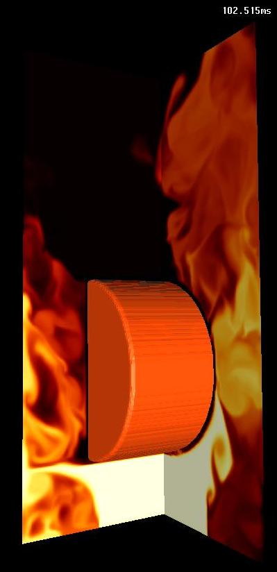
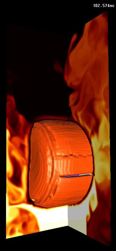
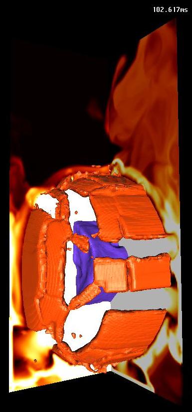
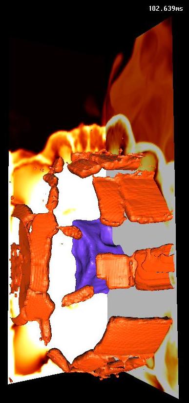
Figure 1: Simulation of exploding cylinder.

The dynamics of the solid materials - steel and PBX 9501 - is modeled using the Lagrangian Material Point Method (MPM) [5]. Gases are generated from solid PBX 9501 using a burn model [9]. Gas-solid interaction is accomplished using an Implicit Continuous Eulerian (ICE) multi-material hydrodynamic code [10]. A single computational grid is used for all the materials.

The constitutive response of PBX 9501 is modeled using ViscoSCRAM [11], which is a five element generalized Maxwell model for the viscoelastic response coupled with statistical crack mechanics. Solid PBX 9501 is progressively converted into a gas with an appropriate equation of state. The temperature and pressure in the gas increase rapidly as the reaction continues. As a result, the steel container is pressurized, undergoes plastic deformation, and finally fragments.

The main issues regarding the constitutive modeling of the steel container are the selection of appropriate models for nonlinear elasticity, plasticity, damage, loss of material stability, and failure. The numerical simulation of the steel container involves the choice of appropriate algorithms for the integration of balance laws and constitutive equations, as well as the methodology for fracture simulation. Models and simulation methods for the steel container are required to be temperature sensitive and valid for large distortions, large rotations, and a range of strain rates (quasistatic at the beginning of the simulation to approximately $10^{6}$ s^-1 at fracture).

The approach chosen for the present work is to use hypoelastic-plastic constitutive models that assume an additive decomposition of the rate of deformation tensor into elastic and plastic parts. Hypoelastic materials are known not to conserve energy in a loading-unloading cycle unless a very small time step is used. However, the choice of this model is justified under the assumption that elastic strains are expected to be small for the problem under consideration and unlikely to affect the computation significantly.

Two plasticity models for flow stress are considered along with a two different yield conditions. Explicit fracture simulation is computationally expensive and prohibitive in the large simulations under consideration. The choice, therefore, has been to use damage models and stability criteria for the prediction of failure (at material points) and particle erosion for the simulation of fracture propagation.

2.1 The Material Point Method

The Material Point Method (MPM)  [5] is a particle method for structural mechanics simulations. In this method, the state variables of the material are described on Lagrangian particles or “material points”. In addition, a regular, structured Eulerian grid is used as a computational scratch pad to compute spatial gradients and to solve the governing conservation equations. An explicit time-stepping version of the Material Point Method has been used in the simulations presented in this paper. The MPM algorithm is summarized below [6].

It is assumed that an particle state at the beginning of a time step is known. The mass ($m$), external force ($\mathbf{f}^{\text{ext}}$), and velocity ($\mathbf{v}$) of the particles are interpolated to the grid using the relations

$$m_{g}=\sum_{p}S_{gp}~{}m_{p}~{},~{}~{}~{}~{}\mathbf{v}_{g}=(1/m_{g})\sum_{p}S_{gp}~{}m_{p}~{}\mathbf{v}_{p}~{},~{}~{}~{}~{}\mathbf{f}^{\text{ext}}_{g}=\sum_{p}S_{gp}~{}\mathbf{f}^{\text{ext}}_{p}$$ (1)

where the subscript ($g$) indicates a quantity at a grid node and a subscript ($p$) indicates a quantity on a particle. The symbol $\sum_{p}$ indicates a summation over all particles. The quantity ($S_{gp}$) is the interpolation function of node ($g$) evaluated at the position of particle ($p$). Details of the interpolants used can be found elsewhere [12].

Next, the velocity gradient at each particle is computed using the grid velocities using the relation

$$\boldsymbol{\nabla}\mathbf{v}_{p}=\sum_{g}\mathbf{G}_{gp}\mathbf{v}_{g}$$ (2)

where $\mathbf{G}_{gp}$ is the gradient of the shape function of node ($g$) evaluated at the position of particle ($p$). The velocity gradient at each particle is used to determine the Cauchy stress ($\boldsymbol{\sigma}_{p}$) at the particle using a stress update algorithm.

The internal force at the grid nodes ($\mathbf{f}^{\text{int}}_{g}$) is calculated from the divergence of the stress using

$$\mathbf{f}^{\text{int}}_{g}=\sum_{p}\mathbf{G}_{gp}~{}\boldsymbol{\sigma}_{p}~{}V_{p}$$ (3)

where $V_{p}$ is the particle volume.

The equation for the conservation of linear momentum is next solved on the grid. This equation can be cast in the form

$$\mathbf{m}_{g}~{}a_{g}=\mathbf{f}^{\text{ext}}_{g}-\mathbf{f}^{\text{int}}_{g}$$ (4)

where $\mathbf{a}_{g}$ is the acceleration vector at grid node ($g$).

The velocity vector at node ($g$) is updated using an explicit (forward Euler) time integration, and the particle velocity and position are then updated using grid quantities. The relevant equations are

$$\mathbf{v}_{g}(t+\Delta t) =\mathbf{v}_{g}(t)+\mathbf{a}_{g}~{}\Delta t$$ (5)

$$\mathbf{v}_{p}(t+\Delta t) =\mathbf{v}_{p}(t)+\sum_{g}S_{gp}~{}\mathbf{a}_{g}~{}\Delta t~{};~{}~{}~{}~{}\mathbf{x}_{p}(t+\Delta t)=\mathbf{x}_{p}(t)+\sum_{g}S_{gp}~{}\mathbf{v}_{g}~{}\Delta t$$ (6)

The above sequence of steps is repeated for each time step. The above algorithm leads to particularly simple mechanisms for handling contact. Details of these contact algorithms can be found elsewhere [13].

2.2 Plasticity and Failure Simulation

A hypoelastic-plastic, semi-implicit approach [14] has been used for the stress update in the simulations presented in this paper. An additive decomposition of the rate of deformation tensor into elastic and plastic parts has been assumed. One advantage of this approach is that it can be used for both low and high strain rates. Another advantage is that many strain-rate and temperature-dependent plasticity and damage models are based on the assumption of additive decomposition of strain rates, making their implementation straightforward.

The stress update is performed in a co-rotational frame which is equivalent to using the Green-Naghdi objective stress rate. An incremental update of the rotation tensor is used instead of a direct polar decomposition of the deformation gradient. The accuracy of model is good if elastic strains are small compared to plastic strains and the material is not unloaded. It is also assumed that the stress tensor can be divided into a volumetric and a deviatoric component. The plasticity model is used to update only the deviatoric component of stress assuming isochoric behavior. The hydrostatic component of stress is updated using a solid equation of state.

Since the material in the container may unload locally after fracture, the hypoelastic-plastic stress update may not work accurately under certain circumstances. An improvement would be to use a hyperelastic-plastic stress update algorithm. Also, the plasticity models are temperature dependent. Hence there is the issue of severe mesh dependence due to change of the governing equations from hyperbolic to elliptic in the softening regime  [15, 16, 17]. Viscoplastic stress update models or nonlocal/gradient plasticity models [18, 19] can be used to eliminate some of these effects and are currently under investigation.

A particle is tagged as “failed” when its temperature is greater than the melting point of the material at the applied pressure. An additional condition for failure is when the porosity of a particle increases beyond a critical limit. A final condition for failure is when a bifurcation condition such as the Drucker stability postulate is satisfied. Upon failure, a particle is either removed from the computation by setting the stress to zero or is converted into a material with a different velocity field which interacts with the remaining particles via contact. Either approach leads to the simulation of a newly created surface.

In the parallel implementation of the stress update algorithm, sockets have been added to allow for the incorporation of a variety of plasticity, damage, yield, and bifurcation models without requiring any change in the stress update code. The algorithm is shown in Algorithm 1. The equation of state, plasticity model, yield condition, damage model, and the stability criterion are all polymorphic objects created using a factory idiom in C++ [20].

Data: Persistent:Initial moduli, temperature, porosity, scalar damage, equation of state, plasticity model, yield condition, stability criterion, damage model

Temporary:Particle state at time $t$

Result: Particle state at time $t+\Delta t$

for all the patches in the domain do

       Read the particle data and initialize updated data storage;

       for all the particles in the patch do

             Compute the velocity gradient, the rate of deformation tensor and the spin tensor;

             Compute the updated left stretch tensor, rotation tensor, and deformation gradient;

             Rotate the input Cauchy stress and the rate of deformation tensor to the material configuration;

             Compute the current shear modulus and melting temperature;

             Compute the pressure using the equation of state, update the hydrostatic stress, and compute the trial deviatoric stress;

             Compute the flow stress using the plasticity model;

             Evaluate the yield function;

             if particle is elastic then

                   Rotate the stress back to laboratory coordinates;

                   Update the particle state;

                  

            else

                   Find derivatives of the yield function;

                   Do radial return adjustment of deviatoric stress;

                   Compute updated porosity, scalar damage, and temperature increase due to plastic work;

                   Compute elastic-plastic tangent modulus and evaluate stability condition;

                   Rotate the stress back to laboratory coordinates;

                   Update the particle state;

                   if Temperature $>$ Melt Temperature or Porosity $>$ Critical Porosity or Unstable then

                         Tag particle as failed;

                        

                   end if

                  

             end if

            

       end for

      

end for

Convert failed particles into a material with a different velocity field;

Algorithm 1 Stress Update Algorithm

2.3 Models

The stress in the solid is partitioned into a volumetric part and a deviatoric part. Only the deviatoric part of stress is used in the plasticity calculations assuming isoschoric plastic behavior.

The hydrostatic pressure ($p$) is calculated either using the bulk modulus ($K$) and shear modulus ($\mu$) or from a temperature-corrected Mie-Gruneisen equation of state of the form [14]

$$p=\frac{\rho_{0}C_{0}^{2}\zeta\left[1+\left(1-\frac{\Gamma_{0}}{2}\right)\zeta\right]}{\left[1-(S_{\alpha}-1)\zeta\right]^{2}+\Gamma_{0}C_{p}T}~{},~{}~{}~{}~{}\zeta=(\rho/\rho_{0}-1)$$ (7)

where $C_{0}$ is the bulk speed of sound, $\rho_{0}$ is the initial density, $\rho$ is the current density, $C_{p}$ is the specific heat at constant volume, $T$ is the temperature, $\Gamma_{0}$ is the Gruneisen’s gamma at reference state, and $S_{\alpha}$ is the linear Hugoniot slope coefficient.

Depending on the plasticity model being used, the pressure and temperature-dependent shear modulus ($\mu$) and the pressure-dependent melt temperature ($T_{m}$) are calculated using the relations [21]

$$\mu =\mu_{0}\left[1+A\frac{p}{\eta^{1/3}}-B(T-300)\right]$$ (8)

$$T_{m} =T_{m0}\exp\left[2a\left(1-\frac{1}{\eta}\right)\right]\eta^{2(\Gamma_{0}-a-1/3)}$$ (9)

where, $\mu_{0}$ is the shear modulus at the reference state($T$ = 300 K, $p$ = 0, $\epsilon_{p}$ = 0), $\epsilon_{p}$ is the plastic strain. $\eta=\rho/\rho_{0}$ is the compression, $A=(1/\mu_{0})(d\mu/dp)$, $B=(1/\mu_{0})(d\mu/dT)$, $T_{m0}$ is the melt temperature at $\rho=\rho_{0}$, and $a$ is the coefficient of the first order volume correction to Gruneisen’s gamma.

We have explored two temperature and strain rate dependent plasticity models - the Johnson-Cook plasticity model [22] and the Mechanical Threshold Stress (MTS) plasticity model [23, 24]. The flow stress ($\sigma_{f}$) from the Johnson-Cook model is given by

$$\sigma_{f}=[A+B(\epsilon_{p})^{n}][1+C\ln(\dot{\epsilon_{p}^{*}})][1-(T^{*})^{m}]~{};~{}~{}\dot{\epsilon_{p}^{*}}=\cfrac{\dot{\epsilon_{p}}}{\dot{\epsilon_{p0}}}~{};~{}~{}T^{*}=\cfrac{(T-T_{r})}{(T_{m}-T_{r})}$$ (10)

where $\dot{\epsilon_{p0}}$ is a user defined plastic strain rate, A, B, C, n, m are material constants, $T_{r}$ is the room temperature, and $T_{m}$ is the melt temperature.

The flow stress for the MTS model is given by

$$\sigma_{f}=\sigma_{a}+\frac{\mu}{\mu_{0}}S_{i}\hat{\sigma}_{i}+\frac{\mu}{\mu_{0}}S_{e}\hat{\sigma}_{e}$$ (11)

where

$$\mu =\mu_{0}-\frac{D}{\exp\left(\frac{T_{0}}{T}\right)-1}$$

$$S_{i} =\left[1-\left(\frac{kT}{g_{0i}\mu b^{3}}\ln\frac{\dot{\epsilon}_{0i}}{\dot{\epsilon}}\right)^{1/qi}\right]^{1/pi}~{};~{}~{}S_{e}=\left[1-\left(\frac{kT}{g_{0e}\mu b^{3}}\ln\frac{\dot{\epsilon}_{0e}}{\dot{\epsilon}}\right)^{1/qe}\right]^{1/pe}$$

$$\theta =\theta_{0}[1-F(X)]+\theta_{IV}F(X)~{};~{}~{}\theta_{0}=a_{0}+a_{1}\ln\dot{\epsilon}+a_{2}\sqrt{\dot{\epsilon}}-a_{3}T$$

$$X =\cfrac{\hat{\sigma}_{e}}{\hat{\sigma}_{es}}~{};~{}~{}F(X)=\tanh(\alpha X)~{};~{}~{}\ln(\hat{\sigma}_{es}/\hat{\sigma}_{es0})=\left(\frac{kT}{\mu b^{3}g_{0es}}\right)\ln\left(\cfrac{\dot{\epsilon}}{\dot{\epsilon}_{es0}}\right)$$

$$\hat{\sigma}_{e}^{(n+1)} =\hat{\sigma}_{e}^{(n)}+\theta\Delta\epsilon$$

and $\sigma_{a}$ is the athermal component of mechanical threshold stress, $\mu_{0}$ is the shear modulus at 0 K, $D,T_{0}$ are empirical constants, $\hat{\sigma}_{i}$ represents the stress due to intrinsic barriers to thermally activated dislocation motion and dislocation-dislocation interactions, $\hat{\sigma}_{e}$ represents the stress due to microstructural evolution with increasing deformation, $k$ is the Boltzmann constant, $b$ is the length of the Burger’s vector, $g_{0[i,e]}$ are the normalized activation energies, $\dot{\epsilon}_{0[i,e]}$ are constant strain rates, $q_{[i,e]},p_{[i,e]}$ are constants, $\theta_{0}$ is the hardening due to dislocation accumulation, $a_{0},a_{1},a_{2},a_{3},\theta_{IV},\alpha$ are constants, $\hat{\sigma}_{es}$ is the stress at zero strain hardening rate, $\hat{\sigma}_{es0}$ is the saturation threshold stress for deformation at 0 K, $g_{0es}$ is a constant, and $\dot{\epsilon}_{es0}$ is the maximum strain rate.

We have decided to focus on ductile failure of the steel container. Accordingly, two yield criteria have been explored - the von Mises condition and the Gurson-Tvergaard-Needleman (GTN) yield condition [25, 26] which depends on porosity. An associated flow rule is used to determine the plastic rate parameter in either case. The von Mises yield condition is given by

$$\Phi=\left(\frac{\sigma_{eq}}{\sigma_{f}}\right)^{2}-1=0~{};~{}~{}~{}\sigma_{eq}=\sqrt{\frac{3}{2}\sigma^{d}:\sigma^{d}}$$ (12)

where $\sigma_{eq}$ is the von Mises equivalent stress, $\sigma^{d}$ is the deviatoric part of the Cauchy stress, and $\sigma^{f}$ is the flow stress. The GTN yield condition can be written as

$$\Phi=\left(\frac{\sigma_{eq}}{\sigma_{f}}\right)^{2}+2q_{1}f_{*}\cosh\left(q_{2}\frac{Tr(\sigma)}{2\sigma_{f}}\right)-(1+q_{3}f_{*}^{2})=0$$ (13)

where $q_{1},q_{2},q_{3}$ are material constants and $f_{*}$ is the porosity (damage) function given by

$$f*=\begin{cases}f&\text{for}~{}~{}f\leq f_{c},\\ f_{c}+k(f-f_{c})&\text{for}~{}~{}f>f_{c}\end{cases}$$ (14)

where $k$ is a constant and $f$ is the porosity (void volume fraction). The flow stress in the matrix material is computed using either of the two plasticity models discussed earlier. Note that the flow stress in the matrix material also remains on the undamaged matrix yield surface and uses an associated flow rule.

The evolution of porosity is calculated as the sum of the rate of growth and the rate of nucleation [27]. The rate of growth of porosity and the void nucleation rate are given by the following equations  [28]

$$\dot{f} =\dot{f}_{\text{nucl}}+\dot{f}_{\text{grow}}$$ (15)

$$\dot{f}_{\text{grow}} =(1-f)\text{Tr}(\mathbf{D}_{p})$$ (16)

$$\dot{f}_{\text{nucl}} =\cfrac{f_{n}}{(s_{n}\sqrt{2\pi})}\exp\left[-\frac{1}{2}\cfrac{(\epsilon_{p}-\epsilon_{n})^{2}}{s_{n}^{2}}\right]\dot{\epsilon}_{p}$$ (17)

where $\mathbf{D}_{p}$ is the rate of plastic deformation tensor, $f_{n}$ is the volume fraction of void nucleating particles , $\epsilon_{n}$ is the mean of the distribution of nucleation strains, and $s_{n}$ is the standard deviation of the distribution.

Part of the plastic work done is converted into heat and used to update the temperature of a particle. The increase in temperature ($\Delta T$) due to an increment in plastic strain ($\Delta\epsilon_{p}$) is given by the equation  [29]

$$\Delta T=\cfrac{\chi\sigma_{f}}{\rho C_{p}}\Delta\epsilon_{p}$$ (18)

where $\chi$ is the Taylor-Quinney coefficient, and $C_{p}$ is the specific heat. A special equation for the dependence of $C_{p}$ upon temperature is also used for steel [30].

$$C_{p}=10^{3}(0.09278+7.454\times 10^{-4}T+12404.0/T^{2})$$ (19)

Under normal conditions, the heat generated at a material point is conducted away at the end of a time step using the heat equation. If special adiabatic conditions apply (such as in impact problems), the heat is accumulated at a material point and is not conducted to the surrounding particles. This localized heating can be used to simulate adiabatic shear band formation.

After the stress state has been determined on the basis of the yield condition and the associated flow rule, a scalar damage state in each material point can be calculated using either of two damage models - the Johnson-Cook model  [31] or the Hancock-MacKenzie model [32]. While the Johnson-Cook model has an explicit dependence on temperature, the Hancock-McKenzie model depends on the temperature implicitly, via the stress state. Both models depend on the strain rate to determine the value of the scalar damage parameter.

The damage evolution rule for the Johnson-Cook damage model can be written as

$$\dot{D}=\cfrac{\dot{\epsilon_{p}}}{\epsilon_{p}^{f}}~{};~{}~{}\epsilon_{p}^{f}=\left[D_{1}+D_{2}\exp\left(\cfrac{D_{3}}{3}\sigma^{*}\right)\right]\left[1+D_{4}\ln(\dot{\epsilon_{p}}^{*})\right]\left[1+D_{5}T^{*}\right]~{};~{}~{}\sigma^{*}=\cfrac{\text{Tr}(\boldsymbol{\sigma})}{\sigma_{eq}}~{};~{}~{}$$ (20)

where $D$ is the damage variable which has a value of 0 for virgin material and a value of 1 at fracture, $\epsilon_{p}^{f}$ is the fracture strain, $D_{1},D_{2},D_{3},D_{4},D_{5}$ are constants, $\boldsymbol{\sigma}$ is the Cauchy stress, and $T^{*}$ is the scaled temperature as in the Johnson-Cook plasticity model.

The Hancock-MacKenzie damage evolution rule can be written as

$$\dot{D}=\cfrac{\dot{\epsilon_{p}}}{\epsilon_{p}^{f}}~{};~{}~{}\epsilon_{p}^{f}=\frac{1.65}{\exp(1.5\sigma^{*})}$$ (21)

The determination of whether a particle has failed can be made on the basis of either or all of the following conditions:

• The particle temperature exceeds the melting temperature.

• The TEPLA-F fracture condition [33] is satisfied. This condition can be written as

  $$(f/f_{c})^{2}+(\epsilon_{p}/\epsilon_{p}^{f})^{2}=1$$ (22)

  where $f$ is the current porosity, $f_{c}$ is the maximum allowable porosity, $\epsilon_{p}$ is the current plastic strain, and $\epsilon_{p}^{f}$ is the plastic strain at fracture.

• An alternative to ad-hoc damage criteria is to use the concept of bifurcation to determine whether a particle has failed or not. Two stability criteria have been explored in this paper - the Drucker stability postulate [34] and the loss of hyperbolicity criterion (using the determinant of the acoustic tensor) [35, 36].

The simplest criterion that can be used is the Drucker stability postulate [34] which states that time rate of change of the rate of work done by a material cannot be negative. Therefore, the material is assumed to become unstable (and a particle fails) when

$$\dot{}\boldsymbol{\sigma}:\mathbf{D}^{p}\leq 0$$ (23)

Another stability criterion that is less restrictive is the acoustic tensor criterion which states that the material loses stability if the determinant of the acoustic tensor changes sign [35, 36]. Determination of the acoustic tensor requires a search for a normal vector around the material point and is therefore computationally expensive. A simplification of this criterion is a check which assumes that the direction of instability lies in the plane of the maximum and minimum principal stress [37]. In this approach, we assume that the strain is localized in a band with normal $\mathbf{n}$, and the magnitude of the velocity difference across the band is $\mathbf{g}$. Then the bifurcation condition leads to the relation

$$R_{ij}g_{j}=0~{};~{}~{}~{}R_{ij}=M_{ikjl}n_{k}n_{l}+M_{ilkj}n_{k}n_{l}-\sigma_{ik}n_{j}n_{k}$$ (24)

where $M_{ijkl}$ are the components of the co-rotational tangent modulus tensor and $\sigma_{ij}$ are the components of the co-rotational stress tensor. If $\det(R_{ij})\leq 0$, then $g_{j}$ can be arbitrary and there is a possibility of strain localization. If this condition for loss of hyperbolicity is met, then a particle deforms in an unstable manner and failure can be assumed to have occurred at that particle.

3 VALIDATION METRICS

The attractiveness of the Taylor impact test arises because of the simplicity and inexpensiveness of the test. A flat-ended cylinder is fired on a target at a large enough velocity and the final deformed shape is measured. The drawback of this test is that intermediate states of the cylinder are difficult to measure and hence are generally not. The validation metrics that we consider in this paper are based on the final shape of the cylinder though other metrics may be considered if measurements of these are made during the course of an impact test. We note that the Taylor test could also be used to validate simulations of dynamic fracture though we do not address that issue in this paper.

There is a large literature on the systematic verification and validation of computational codes (see Oberkampf et al. [38], Babuska and Oden [39] and references therein). It has been suggested that validation metrics be developed that can be used to compare experimental data and simulation results. The metrics discussed in this paper are intended to be a step in that direction but they are not intended to be complete or comprehensive.

The most common metric used in the literature is the “calibrated eyeball” approach or “view-graph norm” (Oberkampf et al. [38]) where a plot of the simulated deformed configuration is superimposed on the experimental data and a subjective judgement of accuracy is made. We believe that there is value to this approach and present all our data in this form. However, we also believe that more quantitative descriptions of the difference between experiment and simulations can be obtained and present comparisons using other metrics.

Metrics, sensitivity studies, and determination of experimental variability are essential. Some quantities of interest are:

1. Metrics

   1. Regression between profiles

   2. Length change

   3. Diameter change

   4. Volume change

   5. Middle bulge difference

   6. Length of elastic zone

   7. plastic strain

   8. temperature

   9. time of impact

   10. energy conversion at impact

2. Sensitivity studies

   1. mesh size (quantify discretization errors)

   2. plasticity model parameters

   3. plasticity model

   4. impact velocity

   5. temperature

   6. length and diameter

3. Variability in experimental data

   1. material

   2. geometry

   3. velocity

   4. temperature

   5. measurement error

4 Taylor impact simulations

In this section, we compare the final deformed shapes from simulations of Taylor impact tests with experimentally obtained data. In cases where images or profiles of the deformed shapes of the cylinders were available, these were digitized using a scanner and then imported into XFig (Sutanthavibul et al. [40]). The scanned images were overlaid with manually digitized lines that were drawn as accurately as possible after expanding the images to a resultion of 1024$\times$1260. The digitized curves were then rotated so that the axes were aligned with the grid. The XFig coordinates were then scaled to length units using cues from the digitized images and their axes (if any were provided). Some small errors (1%-2%) are expected in this procedure. However, the overall profiles of the cylinders are captured accurately in most cases.

The simulations were run for 150 $\mu$s - 200 $\mu$s depending on the problem. The simulation times were chosen such that the cylinders bounced off the anvil and moved away for at least 20 $\mu$s. It was observed at beyond this time, the deformed shape of the cylinder reamined constant and all elastic strains and rotations had been recovered.

In the paper by Carrington and Gayler [41] a highly deformed mild steel specimen has been shown (plate 1, figure 3). To determine if MPM could be used to simulate such large deformations, we ran a Taylor impact test on the problem geometry using the Johnson-Cook plasticity model for 4340 steel. The final deformed shape from Carrington’s paper is compared with our predicted shape in Figure 2. The initial velocity is $V_{0}=2140ft/s=652.3m/s$, the initial diameter of the cylinder is $D_{0}=0.5in=12.7mm$, and the initial length of the cylinder is $L_{0}=0.999in=25.37mm$.

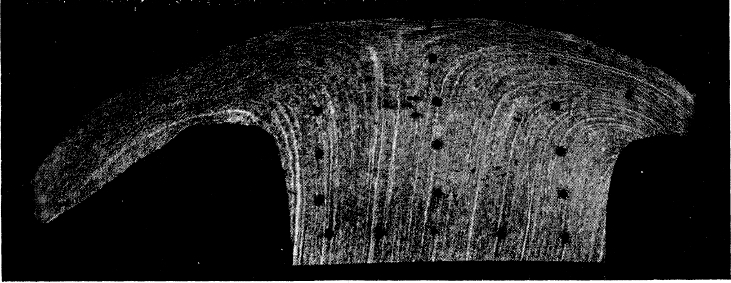
(a) Actual profile (Carrington and Gayler [41]).

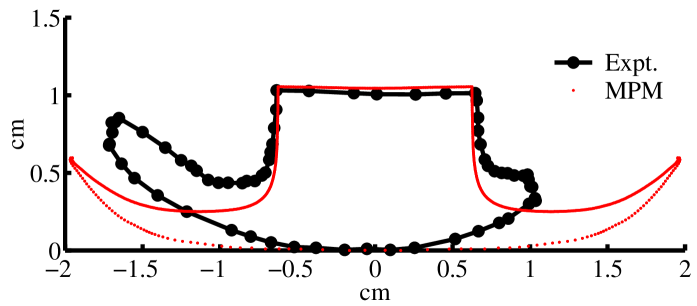
(b) Computed vs. actual profile.

Figure 2: Comparison of experimental vs. computed shapes. $L_{0}$ = 25.37 mm , $D_{0}$ = 12.7 mm, $V_{0}$ = 652.3 m/s.

In our simulation, the 4340 steel cylinder was impacted against a stiff anvil using frictional contact. The 4340 steel flows much more readily than the mild steel used by Carrington and Gayler [41]. The experiment also shows that the tips of the “mushroom” have broken off. We did not simulate any fracture and hence we do not see that effect. However, the overall shape of the deformed specimen suggests that our simulations can provide good qualitative descriptions of large deformations. To quantify how well our simulations fit experimental data, we ran a series of Taylor impact tests on various materials and compared them against experimental data. Some of those results are presented in this report.

4.1 Taylor impact tests on copper

In this section we present the results from Taylor tests on copper specimens for different initial temperatures and impact velocities. Table 1 shows the initial dimensions, velocity, and temperature of the specimens (along with the type of copper used and the source of the data) that we have simulated and compared with experimental data.

Table 1: Initial data for copper simulations. OFHC = oxygen free high conductivity. ETP = electrolytic tough pitch.

Case	Material	Initial	Initial	Initial	Initial	Source
		Length	Diameter	Velocity	Temperature
		($L_{0}$ mm)	($D_{0}$ mm)	($V_{0}$ m/s)	($T_{0}$ K)
Cu-A	OFHC Cu	23.47	7.62	210	298	Wilkins and Guinan [42]
Cu-B	OFHC Cu	25.4	7.62	130	298	Johnson and Cook [22]
Cu-C	OFHC Cu	25.4	7.62	146	298	Johnson and Cook [22]
Cu-D	OFHC Cu	25.4	7.62	190	298	Johnson and Cook [22]
Cu-E	ETP Cu	30	6.00	277	295	Gust [43]
Cu-F	ETP Cu	30	6.00	188	718	Gust [43]
Cu-G	ETP Cu	30	6.00	211	727	Gust [43]
Cu-H	ETP Cu	30	6.00	178	1235	Gust [43]
Cu-I	Annealed Cu.					Zocher et al. [14]
Cu-J	With porosity					Addessio et al. [44]

4.1.1 Room temperature impact of copper

Comparisons between the computed and experimental profiles of annealed copper specimen Cu-I are shown in Figure 3. The MTS model predicts the final length quite accurately (at this is true for other room temperature simulations of copper). The profile shape is also computed accurately. The Johnson-Cook model overestimate the final length. However, the difference is small and may be attributed to material variability.

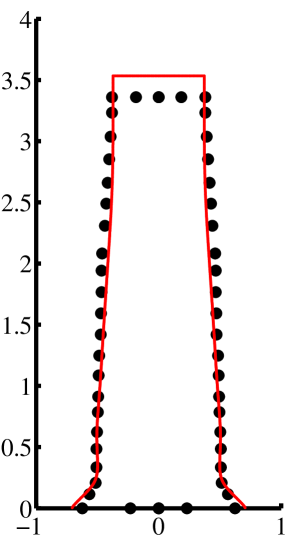
(a) Johnson-Cook.

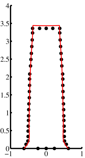
(b) Mechanical Threshold Stress.

Figure 3: Comparison of experimental and computed shapes of annealed copper cylinder Cu-I using the Johnson-Cook and Mechanical Threshold Stress plasticity models. The axes are shown in cm units.

Simulations of impact case Cu-I with increasing mesh refinement are shown in Figure 4. The number of MPM particles is doubled with each refinement. We observe that the solution does not change much as we refine the mesh. However, this is true only at low temperatures and moderate impact velocities. Significant mesh dependence is observed at high temperatures where softening becomes dominant as wee will see in our calculations with 6061-T6 aluminum.

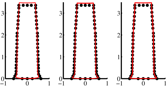
(a) With friction.

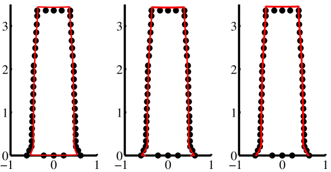
(b) Without friction.

Figure 4: Comparison of experimental and computed shapes of 6061T6 aluminum cylinders using the Johnson-Cook (JC) with increasing mesh refinement. The axes are in cm.

4.1.2 High temperature impact of copper

At higher temperatures, the response of the three plasticity models is quite different. Comparisons between the computed and experimental profiles of ETP copper specimen Cu-F are shown in Figure 5(a), (b), and (c). Those for specimen Cu-G are shown in Figure 5(d), (e), and (f). If frictional contact at the impact surface is simulated, the final shapes of the specimens Cu-F and Cu-G are as shown in Figure 5(g), (h), (i), (j), (k), and (l).

Notice that though both specimens are nominally at the same temperature and has almost identical impact velocities, the final profile is quite different even though the final lengths are nearly identical. It is likely that most of the difference is due the initial conditions with a small contribution from material variability. This conjecture is partially supported by the fact that the profiles predicted by the Johnson-Cook model match the experiments quite well.

We observe that the Johnson-Cook and Steinberg-Guinan models perform well for specimen Cu-F when friction is not included in the calculation. In the presence of frictional contact, the predicted profiles deviate significantly from the experimental profiles in the mushroom region. This indicates that there is a possibility of inaccurate contact force calculation when friction is included.

From specimen Cu-G, the slightly higher impact velocity leads to an underestimation of the final length by the Johnson-Cook model, even though the mushroom region is predicted accurately. The MTS model overestimates the length and underestimates the mushroom diameter while the Steinberg-Guinan model predicts the final length best but fails to predict the mushroom shape. Once again, frictional contact appears to reduce the accuracy of the prediction.

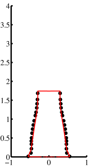
(a) JC (Cu-F).

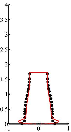
(g) JC (Cu-F) with friction.

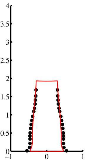
(b) MTS (Cu-F).

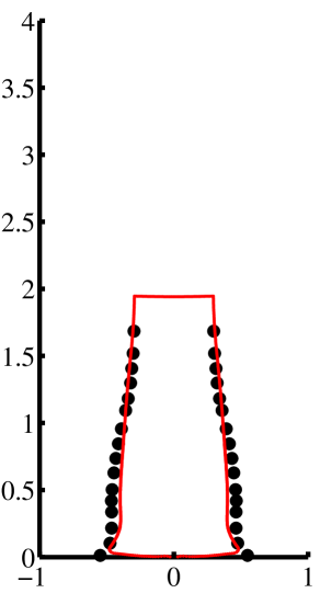
(h) MTS (Cu-F) with friction.

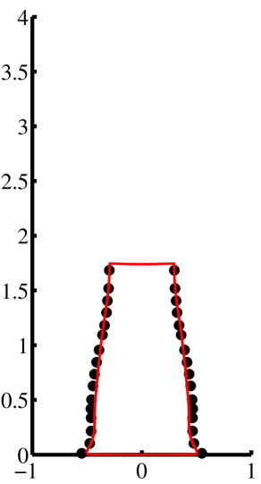
(c) SCG (Cu-F).

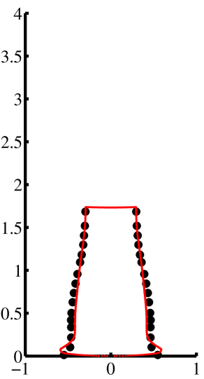
(i) SCG (Cu-F) with friction.

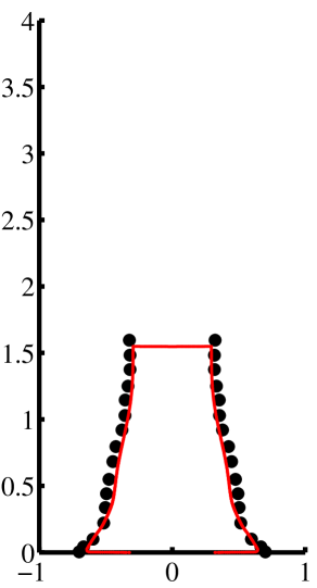
(d) JC (Cu-G).

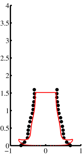
(j) JC (Cu-G) with friction.

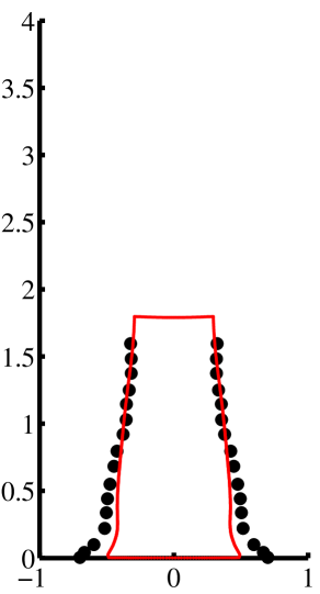
(e) MTS (Cu-G).

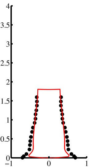
(k) MTS (Cu-G) with friction.

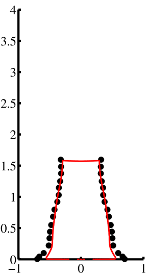
(f) SCG (Cu-G).

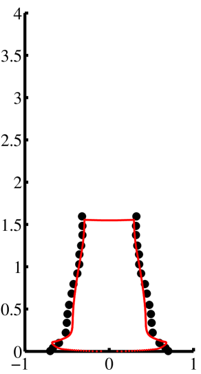
(l) SCG (Cu-G) with friction.

Figure 5: Comparison of experimental and computed shapes of ETP copper cylinders using the Johnson-Cook (JC), Mechanical Threshold Stress (MTS), and Steinberg-Cochran-Guinan (SCG) plasticity models. Specimen C-F has an initial temperature of 718 K and Cu-G is initially at 727 K. The initial velocities are 188 m/s and 211 m/s, respectively. The axes are shown in cm units.

4.1.3 Comparisons with FEM

To determine how our MPM simulations compare with FEM simulations we have run two high temperature ETP copper impact tests using LS-DYNA (with the coupled structural-thermal option). Figure 6 shows the final deformed shapes for the two cases from the MPM and FEM simulations using Johnson-Cook plasticity. In this case frictional contact has been used.

The FEM simulations consistently overestimate the final length of the specimen though the mushroom diameter is more accurately predicted by FEM. For the case where no contact friction is applied, MPM predictions are consistently better than FEM predictions.

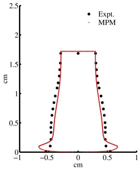
(a) MPM (Cu-F)

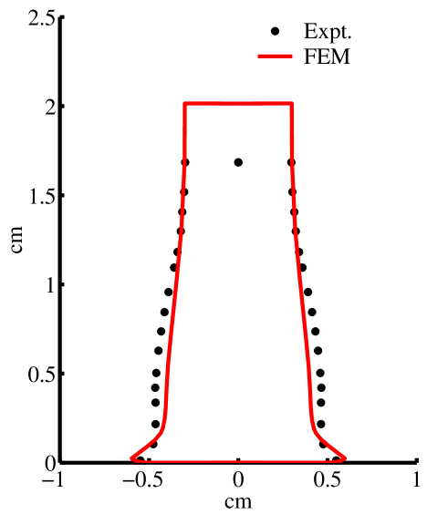
(b) FEM (Cu-F)

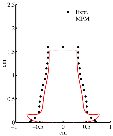
(c) MPM (Cu-G)

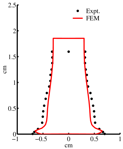
(d) FEM (Cu-G)

Figure 6: Comparison of experimental and computed shapes of ETP copper cylinders using MPM and FEM. The axes are in cm.

4.2 Taylor impact tests on 6061-T6 aluminum alloy

In this section we present the results from Taylor tests on 6061-T6 aluminum specimens for different initial temperatures and impact velocities. We have chosen to study this material as it is a well characterized face centered cubic material that has been utilized by Chhabildas et al. [45] for the validation of high velocity impacts that formed the basis of the second stage of our validation simulations. Table 2 shows the initial dimensions, velocity, and temperature of the specimens (along with the type of copper used and the source of the data) that we have simulated and compared with experimental data.

Table 2: Initial data for 6061-T6 aluminum simulations.

Case	Material	Initial	Initial	Initial	Initial	Source
		Length	Diameter	Velocity	Temperature
		($L_{0}$ mm)	($D_{0}$ mm)	($V_{0}$ m/s)	($T_{0}$ K)
Al-A	6061-T6 Al	23.47	7.62	373	298	Wilkins and Guinan [42]
Al-B	6061-T6 Al	23.47	7.62	603	298	Wilkins and Guinan [42]
Al-C	6061-T6 Al	46.94	7.62	275	298	Wilkins and Guinan [42]
Al-D	6061-T6 Al	46.94	7.62	484	298	Wilkins and Guinan [42]
Al-E	6061-T6 Al	30	6.00	200	295	Gust [43]
Al-F	6061-T6 Al	30	6.00	358	295	Gust [43]
Al-G	6061-T6 Al	30	6.00	194	635	Gust [43]
Al-H	6061-T6 Al	30	6.00	354	655	Gust [43]
Al-I	6061-T6 Al					Addessio et al. [44]

4.2.1 Room temperature impact: 6061-T6 Al

Comparisons between the computed and experimental profiles of 6061T6 aluminum alloy specimen Al-A are shown in Figure 7(a), (b), and (c). Those for specimen Al-C are shown in Figure 7(d), (e), and (f). If frictional contact at the impact surface is simulated, the final shapes of the specimens Al-A and Al-C are as shown in Figure 7 (g), (h), (i), (j), (k), and (l).

We note that all three models predict essentially identical profiles. The higher velocity impact of the shorter specimen Al-A is best predicted by the MTS model as far as final length is concerned. The mushroom width is predicted better when some friction is included at the anvil-specimen interface. There is a noticeable amount of curvature under frictional contact. We believe that this partly due to the contact algorithm that has been used.

The longer specimens have lower impact velocities. However, all three models predict a final length that is shorter than that observed in experiment. We believe that is discrepancy is due to material variability. Note the accuracy with which the profiles are predicted and the noticeably lower curvature of the mushroom under frictional contact compared to specimen Al-A.

(a) JC (Al-A).

(g) JC (Al-A) Friction.

(b) MTS (Al-A).

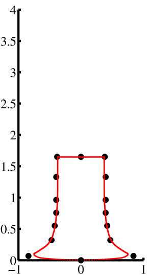
(h) MTS (Al-A) Friction.

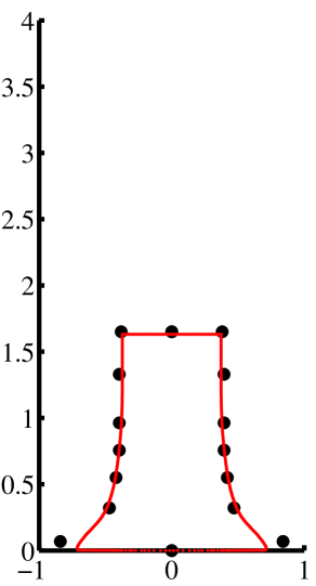
(c) SCG (Al-A).

(i) SCG (Al-A) Friction.

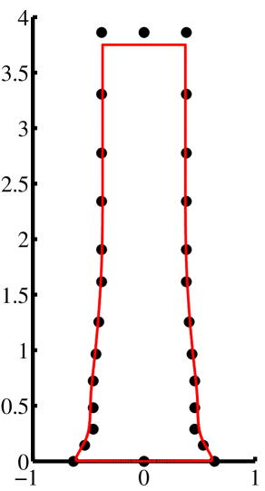
(d) JC (Al-C).

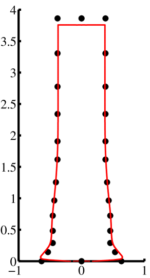
(j) JC (Al-C) Friction.

(e) MTS (Al-C).

(k) MTS (Al-C) Friction.

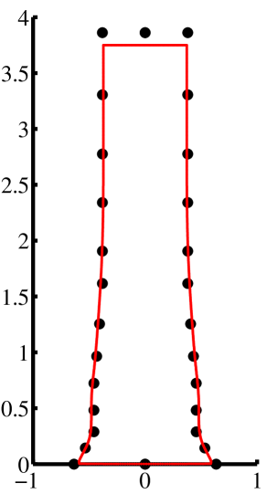
(f) SCG (Al-C).

(l) SCG (Al-C) Friction.

Figure 7: Comparison of experimental and computed shapes of 6061T6 aluminum cylinders using the Johnson-Cook (JC), Mechanical Threshold Stress (MTS), and Steinberg-Cochran-Guinan (SCG) plasticity models. The figure in the top row are from simulations without friction while those in the bottom row are with friction. The axes are shown in cm units.

4.2.2 High temperature impact: 6061-T6 Al

At higher temperatures, the response of the three plasticity models is quite different. Comparisons between the computed and experimental profiles of 6061T6 aluminum alloy specimens have been performed under conditions of frictional contact. The final shapes of the specimens Al-G and Al-H are as shown in Figure 8. If failure simulation is included, the profiles are as shown in Figures 8(g), (h), (i), (j), (k), and (l).

For the lower impact velocity of specimen Al-G, the Johnson-Cook model performs the best at predicting both the final length and the mushroom diameter. Both the MTS and SGC models overestimate the final length and underestimate the mushroom diameter. The MTS model fares slightly worse than the SCG model. However, the differences are small enough that they can be attributed to material variability. Including erosion effects in the simulation does not affect the result significantly.

At the higher impact velocity represented by specimen Al-H, all models fail to predict the final length accurately. The Johnson-Cook model comes closest but overestimates the length and has an excessively deformed mushroom region. The MTS and SCG models have more reasonably shaped mushroom regions but fail to predict the final length by almost 100%. The SCG model is slightly better than the MTS model.

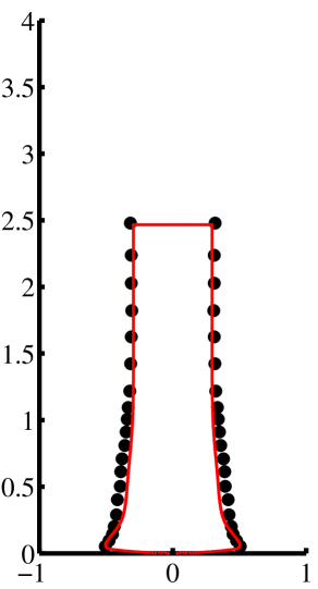
(a) JC (Al-G).

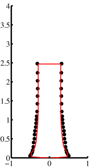
(g) JC (Al-G) with erosion.

(b) MTS (Al-G).

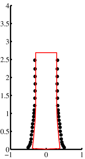
(h) MTS (Al-G) with erosion.

(c) SCG (Al-G).

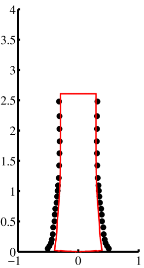
(i) SCG (Al-G) with erosion.

(d) JC (Al-H).

(j) JC (Al-H) with erosion.

(e) MTS (Al-H).

(k) MTS (Al-H) with erosion.

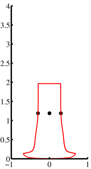
(f) SCG (Al-H).

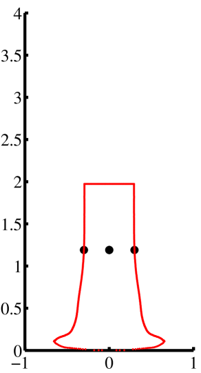
(l) SCG (Al-H) with erosion.

Figure 8: Comparison of experimental and computed shapes of 6061T6 aluminum cylinders using the Johnson-Cook (JC), Mechanical Threshold Stress (MTS), and Steinberg-Cochran-Guinan (SCG) plasticity models. Specimens Al-G and Al-H are both initially at 635 K. Al-G has an impact velocity of 194 m/s while Al-H impacts at 354 m/s. The axes are shown in cm units.

It is possible that the discrepancy that we observe for specimen Al-H is due to inadequate discretization. Simulations of impact specimen Al-H with increasing mesh refinement are shown in Figure 9. The number of grid cells in the plane of the specimen profile has been doubled with each refinement.

If we examine the profiles shown in Figure 9(a), we observe that the cylinder does appear to shorten with increasing refinement. However, there is unphysical curling of the end of the specimen. On the other hand, if we eliminate friction from the calculation, the mushroom appears to increase with increased refinement while the length decreases. This indicates that there is some amount of mesh dependence of the solution that is probably due to the softening behavior of the material.

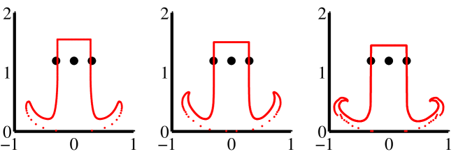
(a) Al-H with friction.

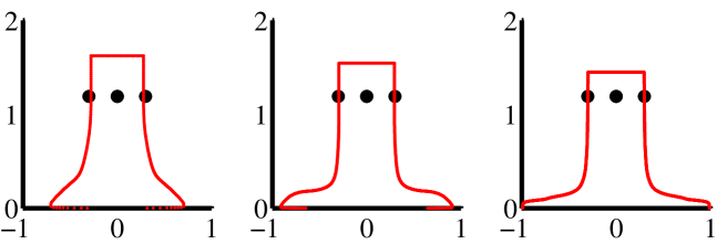
(b) Al-H without friction.

Figure 9: Comparison of experimental and computed shapes of 6061T6 aluminum cylinders (Al-H) using the Johnson-Cook (JC) with increasing mesh refinement. The axes are in cm.

4.2.3 Comparisons with FEM

To determine how our MPM simulations compare with FEM simulations we have run two high temperature aluminum impact tests using LS-DYNA (with the coupled structural-thermal option). Figure 10 shows the final deformed shapes for the two cases from the MPM and FEM simulations using Johnson-Cook plasticity. The FEM simulations consistently overestimate the final length and underestimate the mushroom diameter at high temperatures.

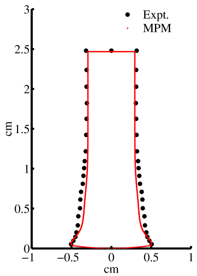
(a) MPM (Al-G)

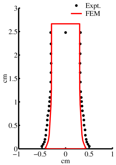
(b) FEM (Al-G)

(c) MPM (Al-H)

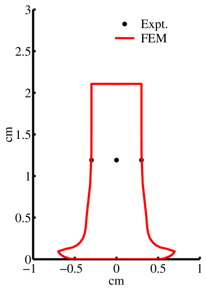
(d) FEM (Al-H)

Figure 10: Comparison of experimental and computed shapes of 6061T6 aluminum cylinders using MPM and FEM. The axes are in cm.

4.3 Taylor impact tests on 4340 steel

In this section we present the results from Taylor tests on 4340 steel specimens for different initial temperatures and impact velocities. Table 3 shows the initial dimensions, velocity, and temperature of the specimens (along with the type of copper used and the source of the data) that we have simulated and compared with experimental data. Note that only a few representative results are shown in this report.

Table 3: Initial data for 4340 steel simulations.

Case	Hardness	Initial	Initial	Initial	Initial	Source
		Length	Diameter	Velocity	Temperature
		($L_{0}$ mm)	($D_{0}$ mm)	($V_{0}$ m/s)	($T_{0}$ K)
St-A	$R_{c}=40$	30	6.00	158	295	Gust [43]
St-B	$R_{c}=40$	30	6.00	232	295	Gust [43]
St-C	$R_{c}=40$	30	6.00	183	715	Gust [43]
St-D	$R_{c}=40$	30	6.00	312	725	Gust [43]
St-E	$R_{c}=40$	30	6.00	136	1285	Gust [43]
St-F	$R_{c}=40$	30	6.00	160	1285	Gust [43]
St-G	$R_{c}=30$	25.4	7.62	208	298	Johnson and Cook [22]
St-H	$R_{c}=30$	12.7	7.62	282	298	Johnson and Cook [22]
St-I	$R_{c}=30$	8.1	7.62	343	298	Johnson and Cook [22]
St-J						Addessio et al. [44]

4.3.1 Room temperature impact: steel

Figure 11 shows the simulated profile of case St-G without friction. The Johnson-Cook model performs quite well in predicting the deformed profile of the specimen. An almost identical profile is obtained if we incorporate friction at the impact surface. Similar results are obtained for the other room temperature specimens.

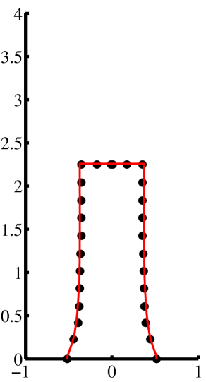
Figure 11: Comparison of experimental and computed shape of 4340 steel cylinder (St-G) without friction. The axes are in cm.

4.3.2 High temperature impact: steel

For high temperature impacts tests, the effect of friction is more obvious in that there is a curling of the edges. Figures 12(a),(b),(c),(d) show the simulated profiles of cases St-D and St-F with friction. Specimen D is at a lower temperature than specimen F but the impact velocity of the form is almost double that of the latter. The Johnson-Cook model predicts the final length of the St-D accurately but underestimates the final length of St-G. This indicates that the high temperature behavior of the model is not quite correct even though the rate dependence is captured well. On the other hand, the Steinberg-Guinan model fails miserably at predicting the high velocity response but does well for the low velocity/high temperature response.

Figures 12(e), (f), (g), and (h) show Taylor impact simulations for cases St-D and St-F with particle erosion. No significant difference can be seen in the computed profiles when we compare these to the plots in Figure 12, except for the SCG model for the St-D sample. Erosion and fracture of the mushroom end does not appear to have a first-order effect on the final length of the impact specimen.

(a) JC (St-D).

(e) JC (St-D) with erosion.

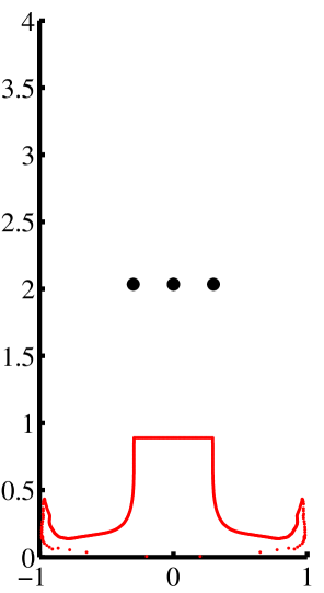
(b) SCG (St-D).

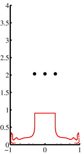
(f) SCG (St-D) with erosion.

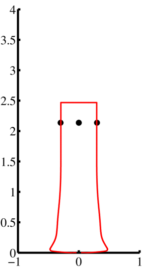
(c) JC (St-F).

(g) JC (St-F) with erosion.

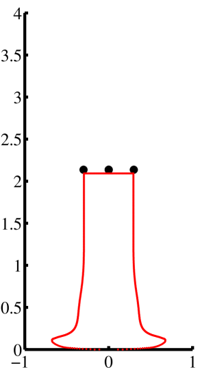
(d) SCG (St-F).

(h) SCG (St-F) with erosion.

Figure 12: Comparison of experimental and computed shapes of 4340 steel cylinder with friction. St-D is at 725 K and 312 m/s. St-F is at 1285 K and 160 m/s. The axes are in cm.

5 CONCLUSION

Lower temperature simulations lead to predicted profiles that are close to those observed in experiment. This is true over a range of impact velocities. However, high temperature impacts do not fare so well.

For the copper specimens, the Johnson-Cook and Steinberg-Guinan models perform better than the MTS model both at low and high temperatures. In future work we show that this is partially due to the stress integration algorithm used in these calculations. Also, FEM simulations consistently overestimate the final length of specimens at high temperatures.

For the aluminum specimens, the three models, Johnson-Cook, MTS and Steinberg-Guinan, predict accurate final lengths and mushroom diameters at room temperature. However, at high temperatures all three models deviate from experiment, especially when the strain rate is increased. This indicates a coupling of strain rate and temperature that is either not captured by these models or requires further calibration. Mesh dependence due to softening appears to be an issue in the MPM simulations. FEM simulations with LS-DYNA predict profiles (at high temperatures) that are less deformed than those predicted by MPM suggesting that the constitutive model evaluation is not as accurate in FEM calculations.

For the steel specimens, both Johnson-Cook and Steinberg-Guinan perform well at room temperature. However, the Steinberg-Guinan model fails under a combination of high impact velocities and high temperatures. The Johnson-Cook model is not very accurate at high temperatures but captures rate-dependent effects quite well. Failure of the material at the mushroom end does not appear to affect the final length of the specimen significantly.

References

- Taylor [1948] G. I. Taylor. The use of flat-ended projectiles for determining dynamic yield stress I. Theoretical considerations. Proc. Royal Soc. London A, 194(1038):289–299, 1948.
- Whiffin [1948] A. C. Whiffin. The use of flat-ended projectiles for determining dynamic yield stress II. Tests on various metallic materials. Proc. Royal Soc. London A, 194(1038):300–322, 1948.
- Johnson and Holmquist [1988] G. R. Johnson and T. J. Holmquist. Evaluation of cylinder-impact test data for constitutive models. J. Appl. Phys., 64(8):3901–3910, 1988.
- Zerilli and Armstrong [1987] F. J. Zerilli and R. W. Armstrong. Dislocation-mechanics-based constitutive relations for material dynamics calculations. J. Appl. Phys., 61(5):1816–1825, 1987.
- Sulsky et al. [1994] D. Sulsky, Z. Chen, and H. L. Schreyer. A particle method for history dependent materials. Comput. Methods Appl. Mech. Engrg., 118:179–196, 1994.
- Sulsky et al. [1995] D. Sulsky, S. Zhou, and H. L. Schreyer. Application of a particle-in-cell method to solid mechanics. Computer Physics Communications, 87:236–252, 1995.
- Armstrong et al. [1999] R. Armstrong, D. Gammon, A. Geist, K. Keahey, S. Kohn, L. McInnes, S. Parker, and B. Smolinski. Toward a Common Component Architecture for high-performance scientific computing. In Proc. 1999 Conference on High Performance Distributed Computing, 1999.
- de St. Germain et al. [2000] J. D. de St. Germain, J. McCorquodale, S. G. Parker, and C. R. Johnson. Uintah: a massively parallel problem solving environment. In Ninth IEEE International Symposium on High Performance and Distributed Computing, pages 33–41. IEEE, Piscataway, NJ, Nov 2000.
- Long and Wight [2002] G. T. Long and C. A. Wight. Thermal decomposition of a melt-castable high explosive: isoconversional analysis of TNAZ. J. Phys. Chem. B, 106:2791–2795, 2002.
- Guilkey et al. [2004] J. E. Guilkey, T. B. Harman, B. A. Kashiwa, and P. A. McMurtry. An Eulerian-Lagrangian approach to large deformation fluid-structure interaction problems. Submitted, 2004.
- Bennett et al. [1998] J. G. Bennett, K. S. Haberman, J. N. Johnson, B. W. Asay, and B. F. Henson. A constitutive model for non-shock ignition and mechanical response of high explosives. J. Mech. Phys. Solids, 46(12):2303–2322, 1998.
- Bardenhagen and Kober [2004] S. G. Bardenhagen and E. M. Kober. The generalized interpolation material point method. Comp. Model. Eng. Sci., 2004. to appear.
- Bardenhagen et al. [2001] S. G. Bardenhagen, J. E. Guilkey, K. M Roessig, J. U. BrackBill, W. M. Witzel, and J. C. Foster. An improved contact algorithm for the material point method and application to stress propagation in granular material. Computer Methods in the Engineering Sciences, 2(4):509–522, 2001.
- Zocher et al. [2000] M. A. Zocher, P. J. Maudlin, S. R. Chen, and E. C. Flower-Maudlin. An evaluation of several hardening models using Taylor cylinder impact data. In Proc. , European Congress on Computational Methods in Applied Sciences and Engineering, Barcelona, Spain, 2000. ECCOMAS.
- Hill and Hutchinson [1975] R. Hill and J. W. Hutchinson. Bifurcation phenomena in the plane tension test. J. Mech. Phys. Solids, 23:239–264, 1975.
- Bazant and Belytschko [1985] Z. P. Bazant and T. Belytschko. Wave propagation in a strain-softening bar: Exact solution. ASCE J. Engg. Mech, 111(3):381–389, 1985.
- Tvergaard and Needleman [1990] V. Tvergaard and A. Needleman. Ductile failure modes in dynamically loaded notched bars. In J. W. Ju, D. Krajcinovic, and H. L. Schreyer, editors, Damage Mechanics in Engineering Materials: AMD 109/MD 24, pages 117–128. American Society of Mechanical Engineers, New York, NY, 1990.
- Ramaswamy and Aravas [1998a] S. Ramaswamy and N. Aravas. Finite element implementation of gradient plasticity models Part I: Gradient-dependent yield functions. Comput. Methods Appl. Mech. Engrg., 163:11–32, 1998a.
- Hao et al. [2000] S. Hao, W. K. Liu, and D. Qian. Localization-induced band and cohesive model. J. Appl. Mech., 67:803–812, 2000.
- Coplien [1992] J. O. Coplien. Advanced C++ Programming Styles and Idioms. Addison-Wesley, Reading, MA, 1992.
- Steinberg et al. [1980] D. J. Steinberg, S. G. Cochran, and M. W. Guinan. A constitutive model for metals applicable at high-strain rate. J. Appl. Phys., 51(3):1498–1504, 1980.
- Johnson and Cook [1983] G. R. Johnson and W. H. Cook. A constitutive model and data for metals subjected to large strains, high strain rates and high temperatures. In Proc. 7th International Symposium on Ballistics, pages 541–547, 1983.
- Follansbee and Kocks [1988] P. S. Follansbee and U. F. Kocks. A constitutive description of the deformation of copper based on the use of the mechanical threshold stress as an internal state variable. Acta Metall., 36:82–93, 1988.
- Goto et al. [2000a] D. M. Goto, J. F. Bingert, W. R. Reed, and R. K. Garrett. Anisotropy-corrected MTS constitutive strength modeling in HY-100 steel. Scripta Mater., 42:1125–1131, 2000a.
- Gurson [1977] A. L. Gurson. Continuum theory of ductile rupture by void nucleation and growth: Part 1. Yield criteria and flow rules for porous ductile media. ASME J. Engg. Mater. Tech., 99:2–15, 1977.
- Tvergaard and Needleman [1984] V. Tvergaard and A. Needleman. Analysis of the cup-cone fracture in a round tensile bar. Acta Metall., 32(1):157–169, 1984.
- Ramaswamy and Aravas [1998b] S. Ramaswamy and N. Aravas. Finite element implementation of gradient plasticity models Part II: Gradient-dependent evolution equations. Comput. Methods Appl. Mech. Engrg., 163:33–53, 1998b.
- Chu and Needleman [1980] C. C. Chu and A. Needleman. Void nucleation effects in biaxially stretched sheets. ASME J. Engg. Mater. Tech., 102:249–256, 1980.
- Borvik et al. [2001] T. Borvik, O. S. Hopperstad, T. Berstad, and M. Langseth. A computational model of viscoplastcity and ductile damage for impact and penetration. Eur. J. Mech. A/Solids, 20:685–712, 2001.
- Goto et al. [2000b] D. M. Goto, J. F. Bingert, S. R. Chen, G. T. Gray, and R. K. Garrett. The mechanical threshold stress constitutive-strength model description of HY-100 steel. Metallurgical and Materials Transactions A, 31A:1985–1996, 2000b.
- Johnson and Cook [1985] G. R. Johnson and W. H. Cook. Fracture characteristics of three metals subjected to various strains, strain rates, temperatures and pressures. Int. J. Eng. Fract. Mech., 21:31–48, 1985.
- Hancock and MacKenzie [1976] J. W. Hancock and A. C. MacKenzie. On the mechanisms of ductile failure in high-strength steels subjected to multi-axial stress-states. J. Mech. Phys. Solids, 24:147–167, 1976.
- Johnson and Addessio [1988] J. N. Johnson and F. L. Addessio. Tensile plasticity and ductile fracture. J. Appl. Phys., 64(12):6699–6712, 1988.
- Drucker [1959] D. C. Drucker. A definition of stable inelastic material. J. Appl. Mech., 26:101–106, 1959.
- Rudnicki and Rice [1975] J. W. Rudnicki and J. R. Rice. Conditions for the localization of deformation in pressure-sensitive dilatant materials. J. Mech. Phys. Solids, 23:371–394, 1975.
- Perzyna [1998] P. Perzyna. Constitutive modelling of dissipative solids for localization and fracture. In Perzyna P., editor, Localization and Fracture Phenomena in Inelastic Solids: CISM Courses and Lectures No. 386, pages 99–241. SpringerWien, New York, 1998.
- Becker [2002] R. Becker. Ring fragmentation predictions using the gurson model with material stability conditions as failure criteria. Int. J. Solids Struct., 39:3555–3580, 2002.
- Oberkampf et al. [2002] W. L. Oberkampf, T. G. Trucano, and C. Hirsch. Verification, validation, and predictive capability in computational engineering and physics. In Verfification and Validation for Modeling and Simulation in Computational Science and Engineering Applications, Johns Hopkins University, Laurel, Maryland, 2002. Foundations for Verfification and Validation in the 21st Century Workshop.
- Babuska and Oden [2004] I. Babuska and J. T. Oden. Verification and validation in computational engineering and science: basic concepts. Comput. Methods Appl. Mech. Engrg., 193:4057–4066, 2004.
- Sutanthavibul et al. [2002] S. Sutanthavibul et al. Xfig User Manual Version 3.2.4. http://www.xfig.org, 2002.
- Carrington and Gayler [1948] W. E. Carrington and M. L. V Gayler. The use of flat-ended projectiles for determining dynamic yield stress III. Changes in microstructure caused by deformation under impact at high-striking velocities. Proc. Royal Soc. London A, 194(1038):323–331, 1948.
- Wilkins and Guinan [1973] M. L. Wilkins and M. W. Guinan. Impact of cylinders on a rigid boundary. J. Appl. Phys., 44(3):1200–1206, 1973.
- Gust [1982] W. H. Gust. High impact deformation of metal cylinders at elevated temperatures. J. Appl. Phys., 53(5):3566–3575, 1982.
- Addessio et al. [1993] F. L. Addessio, J. N. Johnson, and P. J. Maudlin. The effect of void growth on Taylor cylinder impact experiments. J. Appl. Phys., 73(11):7288–7297, 1993.
- Chhabildas et al. [1998] L. C. Chhabildas, C. H. Konrad, D. A. Mosher, W. D. Reinhart, B. D. Duggins, T. G. Trucano, R. M. Summers, and J. S. Peery. A methodology to validated 3D arbitrary Lagrangian Eulerian codes with applications to ALEGRA. Int. J. Impact Engrg., 23:101–112, 1998.