On an exotic Lagrangian torus in $\mathbb{C}P^{2}$

Abstract: We find a non-displaceable Lagrangian torus fiber in a semi-toric system which is superheavy with respect to certain symplectic quasi-state. In particular, this proves Lagrangian $\mathbb{R}P^{2}$ is not a stem in $\mathbb{C}P^{2}$, answering a question of Entov and Polterovich. The main technique we apply is the relation between Lagrangian Floer cohomology and symplectic quasi-morphisms/states due to Fukaya, Oh, Ohta and Ono.

MR(2000) Subject Classification: 53D12; 53D05

1. Introduction

The primary goal of this paper is to understand a toric degeneration model of $\mathbb{C}P^{2}$. Our $\mathbb{CP}^{2}$ model should be considered as a $\mathbb{Z}_{2}$-equivariant version of the one used in [22] for $S^{2}\times S^{2}$. However, we take a slightly different point of view, based on symplectic cuts on cotangent bundles of manifolds with periodic geodesics. This degeneration gives a genuine torus action on an open part of $\mathbb{CP}^{2}$, which results in an interesting family of Lagrangian torus. In particular, such degenerated torus action still gives a moment polytope. For $S^{2}\times S^{2}$, the polytope reads $P_{S^{2}\times S^{2}}=\{(x_{1},x_{2})\in\mathbb{R}^{2}:x_{1},x_{2}\geq 0,x_{1}+2x_{2}\leq 2\}\subset\mathbb{R}^{2}$ (Figure $1$, see [22]). In the case of $\mathbb{CP}^{2}$, one similarly have a toric action on an open set, which gives a moment polytope as in Figure $2$, and can be described as $P_{\mathbb{C}P^{2}}=\{(x_{1},x_{2})\in\mathbb{R}^{2}:x_{1},x_{2}\geq 0,x_{1}+4x_{2}\leq 4\}$.

Figure 1. $S^{2}\times S^{2}$

Figure 2. $\mathbb{C}P^{2}$

In [22], Fukaya-Oh-Ohta-Ono considered the Floer theory of smooth fibers in the toric degeneration model of $S^{2}\times S^{2}$, proving by bulk deformation that there are uncountably many non-displaceable fibers in Figure $1$. In view of Albers-Frauenfelder’s result [2], we may interpret this result as that, only non-displaceable torus fibers below the “monotone level” in the semi-toric system survives the symplectic cut along a level set of $T^{*}S^{2}$. This implies that the anti-diagonal of $S^{2}\times S^{2}$ is not a stem (see 2 for the definition of a stem), answering a question raised by Entov and Polterovich in [14]. This was also proved independently by several other authors [13, 8]. In [13] it was mentioned that Wehrheim also has an unpublished note on this problem.

From Fukaya-Oh-Ohta-Ono’s calculation on $S^{2}\times S^{2}$, we expect the above similar picture of $\mathbb{C}P^{2}$ also contains uncountably many non-displaceable fibers. This would correspond to an easy adaption of Albers-Frauenfelder’s result to $T^{*}\mathbb{R}P^{2}$, by considering the $\mathbb{Z}_{2}$-involution induced by antipodal map on $S^{2}$.

In this paper we find one smooth non-displaceable monotone torus fiber in the moment polytope described above, and prove that it is superheavy with respect to some symplectic quasi-state. In particular, we proved:

Theorem 1.1.

There is a smooth monotone Lagrangian torus fiber in Figure $2$, which is superheavy with respect to certain symplectic quasi-state. In particular, it is stably non-displaceable.

The limitation to such a monotone fiber is due to the difficulty of using $\mathbb{R}P^{2}$ as a bulk to deform our Floer cohomology as in [22], where the bulk is chosen to be an embedded $S^{2}$. Since $\mathbb{RP}^{2}$ only obtains a non-trivial $\mathbb{Z}_{2}$-class, but our calculation shows it is essential that we do not use coefficient ring of characteristic $2$ (see Section 5), the bulk of $\mathbb{RP}^{2}$ does not improve our situation in a straightforward way. The author does not know whether this is only technical. Nonetheless, our computation suffices to show the following:

Corollary 1.2.

$\mathbb{R}P^{2}\subset\mathbb{C}P^{2}$ is not a stem.

This answers the question of Entov-Polterovich ([15], Question 9.2) regarding the case of $\mathbb{C}P^{2}$.

Remark 1.3.

It seems possible that our exotic monotone Lagrangian is in fact the Chekanov torus in $\mathbb{C}P^{2}$. In particular, they both bound $4$ families of disks of Maslov index $2$. It would be nice if one could identify the two geometrically, provided the guess is true. Nonetheless, even if such an identification holds, our calculation still gives new information: we would have an identification of Chekanov torus with a semi-toric fiber and showed the superheaviness of it.

After this work was accomplished, Renato Vianna also detected certain exotic Lagrangian tori in $\mathbb{CP}^{2}$ [35]. His tori can be discerned from the one presented here by the families of holomorphic disks with Maslov number $2$ they bound. It would be interesting to compare the two different objects.

Acknowledgement: The author would like to thank Yong-Geun Oh and Leonid Polterovich for their interests in this work, and many inspiring discussions, which deepens the author’s understandings to this question. The author is indebted to Kenji Fukaya for many interesting comments, as well as pointing out an error in an early draft. The author is also grateful to Chris Wendl for patiently explaining many details of the automatic transversality, to Garrett Alston for drawing the author’s attention to [22], to Matthew Strom Borman for explaining details of symplectic quasi-states, and to Jie Zhao, Ke Zhu for many useful discussions. Part of this work was completed when the author was a graduate student in University of Minnesota under the supervision of Tian-Jun Li. The author is supported by FRG 0244663.

2. Preliminaries

The current section summarizes part of the Lagrangian Floer theory developed by Fukaya-Oh-Ohta-Ono [19, 20, 21] etc, as well as the theory of symplectic quasi-states developed by Entov and Polterovich in a series of their works [17, 14, 15] etc. The aim of this section is to recall basic notions and main framework results in these theories for our applications, as well as for the convenience of readers. Therefore, our scope is rather restricted and will not provide a thorough account to the whole theory. For details and proofs one is refered to the above-mentioned works. Much of our discussions on Lagrangian Floer theory follow the lines of [22].

2.1. Lagrangian Floer theory via potential function

Let $(M,\omega)$ be a smooth symplectic manifold and $L\subset M$ a relatively spin Lagrangian. This means the second Stiefel-Whitney class $w_{2}(L)$ is in the image of the restriction map $H^{2}(M,\mathbb{Z}_{2})\rightarrow H^{2}(L,\mathbb{Z}_{2})$. We first describe the moduli spaces under consideration. Let $J\in\mathcal{J}_{\omega}$, the space of compatible almost complex structures, and $\beta\in H_{2}(M,L;\mathbb{Z})$. We denote by $\mathcal{M}^{\text{main}}_{k+1,l}(\beta;M,L;J)$ as the space of $J$-holomorphic bordered stable maps in class $\beta$ with $k+1$ boundary marked points and $l$ interior marked points. Here, we require the boundary marked points to be ordered counter-clockwisely. When no confusions is likely to occur, we will suppress $M$, $L$ or $J$.

One of the fundamental results in [19] shows that, one has a Kuranishi structure on $\mathcal{M}_{k+1,l}^{\text{main}}(\beta,L)$, so that the evaluation maps at the $i^{\text{th}}$ boundary marked point ($j^{\text{th}}$ interior marked point, respectively)

$$ev_{i}:\mathcal{M}_{k+1,l}^{\text{main}}(\beta,L)\rightarrow L,$$

and

$$ev_{j}^{+}:\mathcal{M}_{k+1,l}^{\text{main}}(\beta,L)\rightarrow M$$

are weakly submersive (see [19] for the definition of weakly submersive Kuranishi maps). For given smooth singular simplices $(f_{i}:P_{i}\rightarrow L)$ of $L$ and $(g_{j}:Q_{j}\rightarrow M)$ of $M$, one can also define the fiber product in the sense of Kuranishi structure:

$$\mathcal{M}_{k+1,l}^{\text{main}}(\beta;L;\overrightarrow{Q},\overrightarrow{P}):=\mathcal{M}_{k+1,l}^{\text{main}}(\beta;L)_{(ev_{1}^{+},\dots,ev_{l}^{+},ev_{1},\dots,ev_{k})\times(g_{1},\dots,g_{l},f_{1},\dots,f_{k})}(\Pi_{j=1}^{l}Q_{j}\times\Pi_{i=1}^{k}P_{i}).$$

The virtual fundamental chain associated to this moduli space,

$$ev_{0}:\mathcal{M}_{k+1,l}^{\text{main}}(\beta;L;\overrightarrow{Q},\overrightarrow{P})\rightarrow L$$

as a singular chain, is defined in [19] via techniques of virtual perturbations.

We consider the universal Novikov rings:

$$\Lambda=\{\sum a_{i}T^{\lambda_{i}}|a_{i}\in\mathbb{C},\lambda_{i}\in\mathbb{R},\lambda_{i}\leq\lambda_{i+1},\lim_{i\rightarrow\infty}\lambda_{i}=\infty\},$$

$$\Lambda_{0}=\{\sum a_{i}T^{\lambda_{i}}|a_{i}\in\mathbb{C},\lambda_{i}\in\mathbb{R}_{\geq 0},\lambda_{i}\leq\lambda_{i+1},\lim_{i\rightarrow\infty}\lambda_{i}=\infty\}.$$

Here $T$ is a formal variable. Consider a valuation which assigns $\sigma_{T}(\sum a_{i}T^{\lambda_{i}})=\lambda_{1}$ if not all $a_{i}=0$, and let $\sigma_{T}(0)=+\infty$. This induces a $\mathbb{R}$-filtration on $\Lambda$ and $\Lambda_{0}$ thus a non-Archimedian topology. Note that $\Lambda_{0}\subset\Lambda$, and $\Lambda_{0}$ has a maximal ideal $\Lambda_{+}$ consisting of elements with $\lambda_{i}>0$ for all $i$. The absence of $e$-variable will reduce the grading of Floer cohomology groups to $\mathbb{Z}_{2}$, but this is irrelevant to our applications.

The heart of Fukaya-Oh-Ohta-Ono’s work is to define a filtered $A_{\infty}$-structure on $C^{*}(L;\Lambda_{0})$ for a Lagrangian $L\subset M$ and define Floer cohomology by deformations of (weak) bounding cochains. However, we will not mention the explicit constructions here, both because they are far beyond our scope, and that there are plenty of comprehensive reference and surveys available in the literature. Just for an incomplete list: [19, 20, 21, 24], etc. Instead we will adopt a most economic approach towards the applications in mind, by recalling a package made available by the deep theory, namely, the computations on Lagrangian Floer cohomology via potential functions.

A potential function $\mathfrak{PO}^{L}$ is a $\Lambda_{+}$-valued function defined on the set of weak bounding cochain of $L$, denoted as $\widehat{\mathcal{M}}_{\text{weak}}(L)$. For any $b\in\widehat{\mathcal{M}}_{\text{weak}}(L)$, one may associate a Floer cohomology group $HF^{*}(L,b)$ for the pair $(L,b)$. We do not define the weak bounding cochains in general, however, according to [22, Remark A.2], $\widehat{\mathcal{M}}_{\text{weak}}(L)$ can be identified with $H^{1}(L;\Lambda_{0})/H^{1}(L;2\pi\sqrt{-1}\mathbb{Z})$ for any monotone Lagrangian submanifolds with minimal Maslov number equal $2$. Hence in the rest of this paper, $\widehat{\mathcal{M}}_{\text{weak}}(L)$ will refer to this particular set, and the potential function can be written as:

(2.1) $$\mathfrak{PO}^{L}:H^{1}(L;\Lambda_{0})/H^{1}(L;2\pi\sqrt{-1}\mathbb{Z})\rightarrow\Lambda_{+}.$$

With the monotonicity assumption above, one may compute $\mathfrak{PO}$ explicitly as in [22, Theorem A.1, A.2]. Choose a basis $\{e_{i}\}_{i=1}^{n}$ for $H^{1}(L;\mathbb{Z})$ and represent $b=\sum_{i=1}^{n}x_{i}e_{i}$ for $b\in H^{1}(L;\Lambda_{0})$ and $x_{i}\in\Lambda_{0}$. Then the potential function is written as:

(2.2) $$\mathfrak{PO}^{L}(b)=\sum_{\mu{\beta}=2}ev_{0}^{*}([\mathcal{M}_{1}(L;J,\beta)])T^{\omega(\beta)/2\pi}exp(b(\partial\beta)).$$

Here $[\partial\beta]\in H_{1}(L;\mathbb{Z})$, hence $b(\partial\beta)\in\Lambda_{0}$. Writing in coordinates, the potential function can be regarded as a function from $(\Lambda_{0}/2\pi\sqrt{-1}\mathbb{Z})^{n}$ to $\Lambda_{+}$. A change of coordinate $y_{i}=e^{x_{i}}$ transforms the function in (2.2) into the form commonly used in the literature:

(2.3) $$\mathfrak{PO}^{L}: \hskip 5.69054pt(\Lambda_{0}\backslash\Lambda_{+})^{n} \rightarrow \hskip 8.53581pt\Lambda_{+}$$

$$(y_{1},\dots,y_{n}) \mapsto \sum_{\mu(\beta)=2}ev_{0}^{*}([\mathcal{M}_{1}(L;J,\beta)])T^{\omega(\beta)/2\pi}y_{i}^{l_{i}},$$

where $\partial\beta=\sum_{i=1}^{n}l_{i}e_{i}^{*}$, for $\{e_{i}^{*}\}_{i=1}^{n}$ a dual basis in $H_{1}(L;\mathbb{Z})$. The following result manifests the importance of potential functions:

Theorem 2.1 ([22], Theorem 2.3).

Let $L$ be a Lagrangian torus in $(M,\omega)$. Suppose that $H^{1}(L;\Lambda_{0})/H^{1}(L;2\pi\sqrt{-1}\mathbb{Z})\subset\widehat{\mathcal{M}}_{\text{weak}}(L)$ and $b\in H^{1}(L;\Lambda_{0})$ is a critical point of the potential function $\mathfrak{PO}^{L}$ of $L$. Then we have:

$$HF^{*}(L,b)\cong H^{*}(L;\Lambda_{0}).$$

In particular, $L$ is non-displaceable.

Remark 2.2.

Results state in this section holds valid for Lagrangians satisfying Condition 6.1 in [22], that is, if any non-empty moduli space of holomorphic disks with Maslov index $\geq 2$. For monotone Lagrangians, there is also an alternative approach developed by Biran and Cornea [7] via pearl complexes, which was used in Vianna’s work [35] and many others.

2.2. Symplectic quasi-states and Lagrangian Floer theory

In this section we briefly review the theory of symplectic quasi-states developed by Entov and Polterovich. A symplectic quasi-state is a functional $\zeta:C^{\infty}(M)\rightarrow\mathbb{R}$ satisfying the following axioms for $H,K\in C^{\infty}(M)$ and $\lambda\in\mathbb{R}$:

1. (Normalization) $\zeta(1)=1$;

2. (Monotonicity) If $H\leq K$, then $\zeta(H)\leq\zeta(K)$;

3. (Quasi-linearity) If $\{H,K\}=0$, then $\zeta(H+\lambda K)=\zeta(H)+\lambda\zeta(K)$;

4. (Vanishing) If supp$(H)$ is displaceable, then $\zeta(H)=0$;

5. (Symplectic invariance) $\zeta(H)=\zeta(H\circ f)$ for $f\in Symp_{0}(M)$

Given a symplectic quasi-state $\zeta$ and a subset $S\subset M$, $S$ is called $\zeta$-heavy if:

$$\zeta(F)\geq\inf_{x\in S}F(x),\hskip 5.69054pt\forall F\in C^{\infty}(M);$$

and $\zeta$-superheavy if

$$\zeta(F)\leq\sup_{x\in S}F(x),\hskip 5.69054pt\forall F\in C^{\infty}(M).$$

One of the basic properties of these subsets proved in [14] is that, a $\zeta$-superheavy subset is always $\zeta$-heavy, and a $\zeta$-heavy set is stably non-displaceable (this is a notion strictly stronger than non-displaceability). Let $V\subset C^{\infty}(M)$ be a finite dimensional linear subspace spanned by pairwisely Poisson-commuting functions. Let $\Psi:M\rightarrow V^{*}$ be the moment map defined by $\langle\Psi(x),F\rangle=F(x)$ for $F\in V$. A non-empty fiber of this moment map is called a stem, if the rest of the fibers are all displaceable. It was essentially proved in Theorem 1.6 of [14] the following:

Theorem 2.3 ([14]).

A stem is a superheavy subset with respect to arbitrary symplectic quasi-states.

In general, the existence of symplectic quasi-states is already an intriguing question. [16] showed that, given a direct sum decomposition of $QH^{*}_{2n}(M)=\mathbb{F}\oplus QH^{\prime}$, where $\mathbb{F}$ is a field, then one may associate a symplectic quasi-state $\zeta_{e}$ to the unit element $e\in\mathbb{F}$.

The relations between symplectic quasi-states and Lagrangian Floer theory are established by the $i$-operator (sometimes also referred to as the open-closed string maps or the Albers map in the literature). The version of $i$-operator we need involves a deformation by the weak bounding cochains, thus denoted as:

$$i^{*}_{b}:QH^{*}(M)\rightarrow HF(L,b).$$

The concrete definition of $i^{*}_{b}$ was given in [19], and we refer interested readers there for details (see also [7] for a similar operator in the context of pearl complexes). The key property of $i^{*}_{b}$ we need is that it sends the unit of $QH^{*}(M)$ to that of $HF(L,b)$. This fact was shown in 7.4.2-7.4.6 in [19], which passes to the so-called canonical model of $C^{*}(L;\Lambda_{0})$ and involved deep algebraic techniques in filtered $A_{\infty}$ algebras, therefore is beyond the scope of the present paper.

With this understood, the key results our proof will rely on reads as follows:

Theorem 2.4 (Theorem 18.8, [25]).

Let $L$ be a relatively spin Lagrangian submanifold of $M$, $b\in\widehat{\mathcal{M}}_{\text{weak}}(L)$ be a weak bounding cochain. $e\in QH^{*}(M;\Lambda)$.

1. If $e\cup e=e$ and $i_{b}^{*}(e)\neq 0$, then $L$ is $\zeta_{e}$-heavy.

2. If $QH^{*}(M;\Lambda)=\Lambda\oplus Q$ is a direct factor decomposition as a ring, and $e$ comes from a unit of the factor $\Lambda$ which satisfies $i^{*}_{b}(e)\neq 0$, then $L$ is $\zeta_{e}$-superheavy.

Corollary 2.5.

Suppose $QH^{*}(M;\Lambda)=\bigoplus_{i=1}^{n}\Lambda e_{i}$ as a ring, for $e_{i}\in QH^{*}(M;\Lambda)$ being a series of idempotents (in particular $QH^{*}$ is semi-simple). If $HF^{*}((L,b);\Lambda)\neq 0$, then $L$ is superheavy for certain symplectic quasi-state $\zeta_{e_{k}}$, $1\leq k\leq n$.

Proof.

This is implicit from the proof of Theorem 23.4, [25]. Since $i^{*}_{qm,b}$ sends the unit to the unit, at least one of the idempotents $e_{k}$ has non-vanishing image. From Theorem 2.4, $L$ is superheavy. ∎

Combining Corollary 2.5, Theorem 2.1 and (2.3), provided we have a semi-simple quantum cohomology ring for the ambient manifold $M$, to show a monotone Lagrangian torus is superheavy with respect to certain symplectic quasi-state, it suffices to compute the contribution of each moduli space of holomorphic disks of Maslov index $2$, and find the critical points for the potential function, which will be the topic of subsequent sections.

3. A semi-toric system of $\mathbb{C}P^{2}$

3.1. Description of the system

We recall the semi-toric system of $\mathbb{C}P^{2}$ particularly suitable for our problem. We first briefly recall the semi-toric model for $S^{2}\times S^{2}$ following the idea of [17] and [34]. Write $S^{2}\times S^{2}$ as

$$\{x_{1}^{2}+y_{1}^{2}+z_{1}^{2}=1\}\times\{x_{2}^{2}+y_{2}^{2}+z_{2}^{2}=1\}\subset\mathbb{R}^{3}\times\mathbb{R}^{3}.$$

Let

$$\widetilde{F}(x_{1},y_{1},z_{1};x_{2},y_{2},z_{2})=z_{1}+z_{2},$$

$$\widetilde{G}(x_{1},y_{1},z_{1};x_{2},y_{2},z_{2})=\sqrt{(x_{1}+x_{2})^{2}+(y_{1}+y_{2})^{2}+(z_{1}+z_{2})^{2}},$$

then

$$\Phi_{S^{2}\times S^{2}}=(F,G):=(\widetilde{F}+\widetilde{G},2-\widetilde{G}):S^{2}\times S^{2}\rightarrow\mathbb{R}^{2}$$

defines a Hamiltonian system. $\widetilde{G}$ is not integrable when it equals $0$, that is, at the anti-diagonal $\bar{\Delta}$. This Hamiltonian system gives a moment polytope as in Figure $1$ up to a rescale of the symplectic form, with a singularity at $(0,1)$ representing a Lagrangian sphere. In classical terms, this is in fact a moment polytope for $S^{2}\times S^{2}\backslash\bar{\Delta}$, where any tubular neighborhood $N(\bar{\Delta})$ of $\bar{\Delta}$ will be mapped into to a neighborhood of $(1,0)$.

Another useful point of view is to consider $S^{2}$ equipped with the standard round metric, which induces a metric on its cotangent bundle. $S^{2}\times S^{2}$ is obtained from $T^{*}S^{2}$ by a symplectic cut at the hypersurface

$$M_{1}=\{p\in T^{*}S^{2}:|p|=1\}.$$

The circle action on this hypersurface is exactly the unit-speed geodesic flow we use for cutting. See [29] for details of the construction of symplectic cuts. In this perspective, we may describe the $\mathbb{T}^{2}$-action induced by $\Phi$ in a geometric way. Consider the rotation of $S^{2}$ along an axis. The cotagent map of this rotation generates the circle action $\tau_{\widetilde{F}}$ on the whole $T^{*}S^{2}$. Another circle action $\tau_{\widetilde{G}}$ is generated by the unit geodesic flow on the complement of the zero section (we already used it for symplectic cut above). Both $\tau_{\widetilde{F}}$ and $\tau_{\widetilde{G}}$ descend under the symplectic cut and commute, thus induces a genuine $\mathbb{T}^{2}$-action on $S^{2}\times S^{2}\backslash\bar{\Delta}$.

We proceed to the case for $\mathbb{C}P^{2}$. Consider the $\mathbb{Z}_{2}$-action on $T^{*}S^{2}$ induced by the antipodal map on the zero section. It is readily seen that, the symplectic cut at the level set $M_{1}$ is also $\mathbb{Z}_{2}$-equivariant, so we may well quotient out this $\mathbb{Z}_{2}$ action first and then perform the symplectic cut. This is equivalent to performing symplectic cut on $T^{*}\mathbb{RP}^{2}$, which results in a symplectic $\mathbb{CP}^{2}$. In summary we have the following commutative diagram, which is equivariant with respect to the action of $\tau_{\tilde{F}}$ and $\tau_{\tilde{G}}$:

Here $\pi$ is the $2$-to-$1$ cover over $T^{*}\mathbb{R}P^{2}$ and $\iota$ is the standard two-fold branched cover from $S^{2}\times S^{2}$ to $\mathbb{C}P^{2}$, branching along the diagonal. Notice now both $\tau_{\tilde{F}}$ and $\tau_{\tilde{G}}$ are $\mathbb{Z}_{2}$-equivariant under the deck transformation, therefore, the above $2$-fold cover induces two commuting circle action on $\mathbb{CP}^{2}\backslash\mathbb{RP}^{2}$. However, since the $\mathbb{Z}_{2}$-action halves the length of each geodesic, to get a time-1 periodic flow, the Hamiltonian function generating the circle action descended from $\tau_{\tilde{G}}$ should be the descendant of $\frac{1}{2}\tilde{G}$ on $S^{2}\times S^{2}$. The end result after approapriate reparametrizations is a toric model for $\mathbb{CP}^{2}\backslash Q$ with moment polytope as in Figure $2$. Note from the reasoning regarding $\tilde{G}$, after the reparametrization the line area of $\mathbb{C}P^{2}$ is $2$ (if the line class area had been $1$, the sizes in Figure $2$ would have been $\frac{1}{2}$ by $2$). Similar to the case of $S^{2}\times S^{2}$, $(1,0)$ indeed represents the standard Lagrangian $\mathbb{RP}^{2}\subset\mathbb{CP}^{2}$. We will denote this semi-toric moment map as $\Phi_{\mathbb{C}P^{2}}$.

3.2. Symplectic cutting $\mathbb{C}P^{2}$

The main ingredient of our proof, following an idea of the arxiv version of [22], is to split $\mathbb{C}P^{2}$ into two pieces and glue the holomorphic curves. The splitting we use is described as follows. We continue to regard $\mathbb{C}P^{2}$ as a result of cutting along $M_{1}$ in $T^{*}\mathbb{R}P^{2}$. Consider $M_{\epsilon}=\{|p|=\epsilon\}\subset T^{*}\mathbb{R}P^{2}\hookrightarrow\mathbb{C}P^{2}$. A further symplectic cut along $M_{\epsilon}$ results in two pieces, and we examine this cutting in slightly more detailed.

Let $X_{0}$, $X_{1}$ be the two components of $\mathbb{C}P^{2}\backslash M_{\epsilon}$, where $X_{1}$ contains the original $\mathbb{R}P^{2}$. Their closure, denoted $X^{\prime}_{0}$ and $X^{\prime}_{1}$, respectively, has a boundary being the lens space $L(4,1)$ equipped with the standard contact form (the one coming from $S^{3}$ quotiented by a $\mathbb{Z}_{4}$-action), and therefore a local $S^{1}$-action of the neighborhood.

As is constructed in [29], by quotienting such an action on $\partial X_{1}$ and gluing back to $X^{\prime}_{1}$, one completes the symplectic cutting and this operation results in $X^{\prime\prime}_{1}:=(\mathbb{C}P^{2},2\epsilon\omega_{0})$. Denote $H\in H_{2}(\mathbb{CP}^{2},\mathbb{Z})$ as the homology class of a line, then $X^{\prime\prime}_{1}\backslash X_{1}$ is an embedded symplectic divisor in $X^{\prime\prime}_{1}$ of class $2H$, which we called the cut locus or cut divisor. The same procedure on the other piece $X_{0}$ leads to a minimal symplectic $4$-manifold (see for example Lemma $1.1$ in [11]), along with a symplectic sphere of self-intersection $(+4)$ inherited from the quadric $Q:=\{x^{2}+y^{2}+z^{2}=0\}$ in the original $\mathbb{C}P^{2}$. Moreover, it contains a symplectic sphere of self-intersection $(-4)$ as cut locus, from which we see $X^{\prime\prime}_{0}$ is indeed the symplectic fourth Hirzebruch surface $F_{4}$ by McDuff’s famous classification of rational and ruled manifolds [32].

We also want to examine such a cut process from the other side of $M_{1}$. Biran’s decomposition theorem for $\mathbb{C}P^{2}$ ([3]) implies that $\mathbb{C}P^{2}\backslash\mathbb{R}P^{2}$ is indeed a symplectic disk bundle $\mathcal{O}(4)$ over a sphere, where the zero section has symplectic area $4$, and the symplectic form is given by $\pi^{*}\omega_{\Sigma}+d(\bar{r}^{2}\alpha)$. Here $\pi$ is the projection to the zero section, $\omega_{\Sigma}$ a standard symplectic form on the sphere up to a rescale, $\bar{r}$ the radial coordinate of the fiber and $\alpha$ a connection form of the circle bundle associated to $\mathcal{O}(4)$. Then the fiber class has at most symplectic area $1$, and the total space can be identified symplectically with $\mathbb{C}P^{2}\backslash\mathbb{R}P^{2}$ with the standard sympletic form.

In this case $X^{\prime}_{0}$ is identified with $\{|\bar{r}|\leq 1-\epsilon\}\subset\mathcal{O}(4)$ and the geodesic flow in $T^{*}\mathbb{R}P^{2}$ is identified with the action of the one obtained by multiplying $e^{i\theta}$ in each fiber. Therefore, one may perform a symplectic cut along $|\bar{r}|=1-\epsilon$ for $1\gg\epsilon>0$, the resulting manifold is again the symplectic $F_{4}$ as above, where the form is compatible with the standard (integrable) complex structure obtained as $P(\mathcal{O}\oplus\mathcal{O}(4))$. To summarize, we have the following (see also Figure $3$):

Lemma 3.1.

Consider $\mathbb{C}P^{2}$ as a consequence of symplectic cut along the contact type hypersurface $\{|p|=1\}\subset T^{*}\mathbb{R}P^{2}$. Then a further symplectic cut along $\{|p|=\epsilon\}$ results in a $\mathbb{C}P^{2}$ with rescaled symplectic form, as well as a symplectic fourth Hirzebruch surface whose zero section has symplectic area equal $2$. Moreover, the symplectic $\mathbb{C}P^{2}$ comes naturally with a symplectic quadric as the cut locus, and $F_{4}$ with a $(-4)$-sphere as cut locus.

Remark 3.2.

Discussions above seem to be well-known. For a dual perspective via symplectic fiber sum, one is referred to for example [11]. In particular, the above cutting can be seen as a reverse procedure of symplectic rational blow-down of the $(-4)$-sphere in the symplectic $F_{4}$.

Figure 3. Cutting along $M_{\epsilon}$

3.3. Second homology classes of $\mathbb{C}P^{2}$ with boundary on a semi-toric fiber

From Section 3.1, we have obtained a desired family of Lagrangian torus as semi-toric fibers in $\mathbb{CP}^{2}$. From now on $L$ will denote one of the semi-toric fibers parametrized by $\mathbb{R}^{2}$-coordinates in Figure 2. Our next task is to understand $H_{2}(\mathbb{CP}^{2},L)$.

From the usual long exact sequence for relative homology, one easily sees that $H_{2}(\mathbb{C}P^{2},L;\mathbb{Z})$ has rank $3$. Again split $\mathbb{CP}^{2}$ along $M_{\epsilon}$ into a copy of $F_{4}$ and $(\mathbb{CP}^{2},\epsilon\omega_{std})$ as in Section 3.2, while keeping $L\subset F_{4}$ by choosing $\epsilon$ small enough.

From the classification theorem of homology classes in [10], one obtains eight homology classes of interests, marked as $[D_{i}]$ and $[e_{i}]$, $i=1,2,3,4$ as Figure $4$ below. In the figure, $e_{i}$ are the $\mathbb{T}^{2}$-equivariant divisors and, as relative cycles, $D_{i}$ denote the image of $J_{0}$-holomorphic disks which intersects $e_{j}$ exactly $\delta_{ij}$ times counting multiplicity. For ease of drawing we did not draw $D_{3}$ perpendicular to $e_{3}$, but it is understood in the way of how Cho and Oh described in [10].

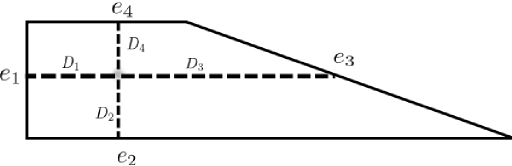
Figure 4. $H_{2}(F_{4},L;\mathbb{Z})$

Out of these eight classes, one has a basis of $H_{2}(F_{4},L;\mathbb{Z})$ consisting of $[e_{1}]$, $[e_{2}]$, $[D_{1}]$ and $[D_{2}]$. Other classes have relations

(3.1) $$[e_{3}]=[e_{1}],\hskip 5.69054pt[e_{4}]=[e_{2}]-4[e_{1}],$$

(3.2) $$[D_{1}]+[D_{3}]+4[D_{2}]=[e_{2}],\hskip 5.69054pt[D_{2}]+[D_{4}]=[e_{1}].$$

On way of checking these relations is to use Poincare pairings and gluing chains with opposite boundaries on $L$. Notice that there is a natural homomorphism by restriction to the Borel-Moore homology of $F_{4}\backslash e_{4}$:

$$\iota:H_{2}(F_{4},L;\mathbb{Z})\rightarrow H_{2}^{BM}(F_{4}\backslash e_{4},L;\mathbb{Z}).$$

$\iota$ is surjective with kernel $[e_{4}]$, so the classes in $H_{2}^{BM}(F_{4}\backslash e_{4},L;\mathbb{Z})$ can still be represented by $e_{i}$, $i=1,2,3$ and $D_{j}$, $j=1,2,3,4$ appropriately punctured with the same relations as in (3.1), (3.2). These facts can be easily seen from the duality between the Borel-Moore homology and the usual cohomology.

On the other side of the cutting, which is $\mathbb{C}P^{2}\backslash Q$, where $Q=\{x^{2}+y^{2}+z^{2}=0\}$ being the standard quadric, the second Borel-Moore homology contains only a $2$-torsion. We will only consider Borel-Moore cycles with asymptotics equal a union of certain Reeb orbits of $\partial^{\infty}(\mathbb{C}P^{2}\backslash Q)=L(4,1)$. Regard Borel-Moore cycles with $2k$ punctures (number of Reeb orbits) at infinity as equivalent, and denote such equivalence classes by $kH^{\prime}$. Note that $k$ already contains information of the homology classes: cycles in $k_{1}H^{\prime}$ and $k_{2}H^{\prime}$ represent the same Borel-Moore classes in $H_{2}(\mathbb{CP}^{2}\backslash Q,\partial^{\infty}(\mathbb{CP}^{2}\backslash Q))$ if and only if $k_{1}-k_{2}\equiv 0$ mod$2$, but the relative chern number will depend on the actual equivalence classes instead of solely the Borel-Moore classes. See Section 3.4.

Relations between classes in $X_{0}=F_{4}\backslash e_{4}$ and $X_{1}=\mathbb{C}P^{2}\backslash Q$: To describe the relations between classes in the two pieces, we first fix a basis of $H_{2}^{BM}(F_{4}\backslash e_{4},L;\mathbb{Z})$ consisting of $\{\iota[e_{2}],\iota[D_{1}],\iota[D_{2}],\iota[D_{4}]\}$. When no possible confusion occurs, we will simply suppress $\iota$ by abuse of notation. Notice that cycles in $kH^{\prime}$ in $X_{1}$ has $2k$ punctures counting multiplicity, which matches with cycles with coefficient $2k$ in the $D_{4}$-component in $X_{0}$. Of particular interests, by matching a cycle $C_{H^{\prime}}\subset X_{1}$ in class $H^{\prime}$ with a $2$-cycle of class $2[D_{4}]$ with correct asymptotics, one obtains a relative cycle in $\mathbb{C}P^{2}$ with boundary on $L$. The class in $H_{2}(\mathbb{C}P^{2},L;\mathbb{Z})$ represented by such a cycle is denoted as $[D^{\prime}_{4}]=2[D_{4}]\#[H^{\prime}]$.

To understand $[D_{4}^{\prime}]$ more explicitly, notice that $\partial[D^{\prime}_{4}]=2\partial[D_{4}]=-2\partial[D_{2}]\in H_{1}(L;\mathbb{Z})$. Therefore, one may match a cycle in class $[D^{\prime}_{4}]$ with one in $2[D_{2}]$ to obtain a closed cycle in $\mathbb{C}P^{2}$. Such a cycle intersects $e_{2}$ positively twice counting multiplicities, and therefore represents nothing but class $H\in H_{2}(\mathbb{C}P^{2};\mathbb{Z})$. In summary, we deduced that:

(3.3) $$[H^{\prime}]\#2[D_{4}]\#2[D_{2}]=[D_{4}^{\prime}]\#2[D_{2}]=H\in H_{2}(\mathbb{C}P^{2};\mathbb{Z})$$

Classes $[e_{1}]$ and $[e_{3}]$ does not extend naturally to closed classes as in $H_{2}(\mathbb{C}P^{2})$. However, as what we did to $[D_{4}]$, twice of them caps cycles in $H^{\prime}$ of $X_{1}$. Therefore we also have:

(3.4) $$[H^{\prime}]\#2[e_{1}]=[H^{\prime}]\#2[e_{3}]=H\in H_{2}(\mathbb{C}P^{2};\mathbb{Z})$$

These gluing relations will play an important role later. It is also readily seen that $\{H,[D_{1}],[D_{2}]\}$ forms a basis of $H_{2}(\mathbb{C}P^{2},L;\mathbb{Z})$, where $F_{4}\backslash e_{4}$ is (symplectically) embedded to $\mathbb{C}P^{2}$ in a canonical way, thus induces a natural inclusion of Borel-Moore two cycles.

3.4. Computation of the relative Chern numbers and Conley-Zehnder indices

We now compute the Maslov indices for $H_{2}(\mathbb{CP}^{2},L)$ by understanding the relative Chern classes and Conley-Zehnder indices involved. A technical reason which makes our case slightly more complicated than the case of a Lagrangian $S^{2}$ is that there is no natural splitting of $T(T^{*}\mathbb{R}P^{2})$. This is caused by the non-orientability of $\mathbb{R}P^{2}$ (to compare the case of Lagrangian $S^{2}$, see for example [26, 18, 31]). However, we will use a trivialization of the splitting surface $M_{\epsilon}$ which seems even more natural and convenient in the (semi-)toric context.

As we already saw, there is an $S^{1}$-action on $\partial X^{\prime}_{i}=M_{\epsilon}$ for both $i=0,1$. In the toric picture of $\mathbb{C}P^{2}\backslash\mathbb{R}P^{2}$, such an $S^{1}$-action induces a vector field on $M_{\epsilon}$ which is dual to $\frac{\partial}{\partial x_{2}}$ in the moment polytope. This action induces a natural trivialization of the contact distribution over its own orbits. We will call such a trivialization $\Phi$ and use it to compute the Conley-Zehnder indices and first Chern numbers. For the definitions of these two invariants one is referred to [12], or [18, 26]

By definition, the Poincare return map with respect to such a trivialization is always identity, therefore,

(3.5) $$\mu^{\Phi}_{CZ}\equiv 0.$$

We will pursue the first Chern number for (Borel-Moore) classes described in Section 3.3 in the rest of the section.

We start with $X_{0}$. As always we assume the Lagrangian torus fiber is contained in this side. Consider again the $\mathcal{O}(4)$ disk bundle as in Section 3.2, from which we cut along another hypersurface $M_{\epsilon/2}=\{r=1-\frac{\epsilon}{2}\}$ to obtain a symplectic fourth Hirzebruch surface $\overline{X}_{0}$. One may also equip it a compatible toric complex structure. The anti-canonical divisor is defined by the equivariant divisors on the boundary of the moment polytope, therefore, the anti-canonical line bundle $\bigwedge^{2}T\overline{X}_{0}$ admits an equivariant section $\xi$ vanishing exactly on the boundary equivariant divisors with order $1$.

Embed $X_{0}$ equivariantly into $\overline{X}_{0}$. Take any cycle $u:\Sigma\rightarrow X_{0}$ with boundary on a torus fiber $L$ and asymptotics being Reeb orbits of $\partial X_{0}$. It has boundary Maslov index zero if we take the trivialization induced by the torus action near $L$. Assume that $u$ intersects transversally with the equivariant divisors. The pull-back $u^{*}\bigwedge^{2}(TX_{0},J)$ thus comes naturally with a section $u^{*}\xi$ which vanishes at $u(\Sigma)\cap\bigcup_{i=1}^{4}e_{i}$ with order $\pm 1$ depending on the intersection form. $u^{*}\xi$ is clearly equivariant with the $S^{1}$-action on $\partial X_{0}$ and the torus boundary thus agreeing with the trivialization there. This observation computes immediately the following:

(3.6) $$c_{1}^{\Phi}(D_{1})=c_{1}^{\Phi}(D_{2})=c_{1}^{\Phi}(D_{3})=1,\hskip 5.69054ptc_{1}^{\Phi}(D_{4})=0.$$

Notice also that the first chern number of $e_{2}$ is independent of the choice of trivializations. From (3.1) and (3.2) we may compute the rest of the chern numbers summarized as follows:

(3.7) $$c_{1}^{\Phi}(e_{1})=c_{1}^{\Phi}(e_{3})=1,\hskip 5.69054ptc_{1}^{\Phi}(e_{2})=6.$$

For the relative Chern classes in $X_{1}$, we again focus on cycles with asymptotics equal copies of $S^{1}$-orbits on $M_{\epsilon}$. Note that, when counting multiplicity, there are always even number of $S^{1}$-orbits since simple orbits represents a non-trivial element in $\pi_{1}(T^{*}\mathbb{R}P^{2})$. The class $kH^{\prime}$ has $2k$ asymptotics, which can be capped by $2k[D_{4}]\#2k[D_{2}]$ to form a closed cycle in $\mathbb{C}P^{2}$ from 3.2. Such a class intersects positively with $e_{2}$ at $2k$ points, thus itself being the class $kH$ in $\mathbb{C}P^{2}$. From our computation in $X_{0}$, we see that

(3.8) $$c_{1}^{\Phi}(kH^{\prime})=3k-2k=k>0.$$

4. Classification of Maslov $2$ disks

4.1. A quick review on SFT and neck-stretching

In this section we collect basic definitions and facts from symplectic field theory, especially the part of neck-stretching, mostly for readers’ convenience and to fix notations. For more details, we refer interested readers to [12], [5], and other expositions such as [18, 26, 31].

Given a closed symplectic manifold $(M,\omega)$, we call $(N,\alpha)$ a contact type hypersurface if there is a neighborhood $V$ of $N$, such that $V$ is diffeomorphic to $(-\epsilon,\epsilon)\times N$, and $\partial_{s}$ is a Liouville vector field in $V$, that is, $\mathcal{L}_{\partial_{s}}\omega=\omega$. Here $s$ is the coordinate of the first component of $U$. In this case, $\alpha=i_{\partial_{s}}\omega$ is a contact form, of which the contact distribution is denoted $\xi$, and the Reeb flow denoted by $R$.

An almost complex structure $J\in\mathcal{J}_{\omega}$ is called adjusted if the following conditions hold in $U$:

1. $J|_{\xi}=\widetilde{J}$ is independent of $s$;

2. $J(\partial_{s})=R$.

We now consider a deformation of a given adjusted almost complex structure $J$. Let $V_{t}=[-t-\epsilon,t+\epsilon]$ and $\beta_{t}:V_{t}\rightarrow[-\epsilon,\epsilon]$ be a strictly increasing function with $\beta_{t}(s)=s+t$ on $[-t-\epsilon,-t-\epsilon/2]$ and $\beta_{t}(s)=s-t$ on $[t+\epsilon/2,t+\epsilon]$. Define a smooth embedding $f_{t}:V_{t}\times N\hookrightarrow M$ by:

$$f_{t}(s,m)=(\beta_{t}(s),m).$$

Let $\bar{J}_{t}$ be the ${\partial\over\partial s}-$invariant almost complex structure on $V_{t}\times N$ such that $\bar{J}_{t}({\partial\over\partial s})=R$ and $\bar{J}_{t}|_{\xi}=J|_{\xi}$. Glue the almost complex manifold $(M\backslash f_{t}(V_{t}\times N),J)$ to $(V_{t}\times N,\bar{J}_{t})$ via $f_{t}$ to obtain the family of almost complex structures $J_{t}$ on $M$.

Notice that each $J_{t}$ agrees with $J$ away from the collar $(-\epsilon,\epsilon)\times H$. And on this collar, it agrees with $J$ on $\xi$. Suppose $N$ is separating, denote $M\backslash N=W\cup U$, where $W$ has a concave boundary and $U$ a convex boundary. When $i\to\infty$ the neck-stretching process results in an almost complex structure $J_{\infty}$ on the union of symplectic completions $\overline{W}=(-\infty,0]\times N\cup W$ of $W$ and $\overline{U}=U\cup[0,+\infty)$ of $U$. On the cylindrical ends, we require $J|_{\infty}(\partial_{s})=R$ and $J|_{\infty}=J|_{\xi}$ similar to the definition of $\overline{J}_{t}$. In an exact same way, we define $J_{\infty}$ on $SN=((-\infty,+\infty)\times N,d(e^{t}\alpha))$, the symplectization of $N$.

Let $M_{\infty}=\overline{W}\cup SN\cup\overline{U}$, and $J_{\infty}$ be the almost complex structure defined above. Let $\Sigma$ be a Riemann surface with nodes. A level-$k$ holomorphic building consists of the following data:

1. (level) A labelling of the components of $\Sigma\backslash\{\text{nodes}\}$ by integers $\{1,\cdots,k\}$ which are the levels. Two components sharing a node differ at most by $1$ in levels. Let $\Sigma_{r}$ be the union of the components of $\Sigma\backslash\{\text{nodes}\}$ with label $r$.

2. (asymptotic matching) Finite energy holomorphic curves $v_{1}:\Sigma_{1}\rightarrow U$, $v_{r}:\Sigma_{r}\rightarrow SN$, $2\leq r\leq k-1$, $v_{k}:\Sigma_{k}\rightarrow W$. Any node shared by $\Sigma_{l}$ and $\Sigma_{l+1}$ for $1\leq l\leq k-1$ is a positive puncture for $v_{l}$ and a negative puncture for $v_{l+1}$ asymptotic to the same Reeb orbit $\gamma$. $v_{l}$ should also extend continuously across each node within $\Sigma_{l}$.

Now for a given stretching family $\{J_{t_{i}}\}$ as previously described, as well as $J_{t_{i}}$-curves $u_{i}:S\rightarrow(M,J_{t_{i}})$, we define the Gromov-Hofer convergence as follows:

A sequence of $J_{t_{i}}$-curves $u_{i}:S\rightarrow(M,J_{t_{i}})$ is said to be convergent to a level-$k$ holomorphic building $v$ in Gromov-Hofer’s sense, using the above notations, if there is a sequence of maps $\phi_{i}:S\rightarrow\Sigma$, and for each $i$, there is a sequence of $k-2$ real numbers $t_{i}^{r}$, $r=2,\cdots,k-1$, such that:

1. (domain) $\phi_{i}$ are locally biholomorphic except that they may collapse circles in $S$ to nodes of $\Sigma$,

2. (map) the sequences $u_{i}\circ\phi_{i}^{-1}:\Sigma_{1}\rightarrow U$, $u_{i}\circ\phi_{i}^{-1}+t_{i}^{r}:\Sigma_{r}\rightarrow SH$, $2\leq r\leq k-1$, and $u_{i}\circ\phi_{i}^{-1}:\Sigma_{k}\rightarrow W$ converge in $C^{\infty}$-topology to corresponding maps $v_{r}$ on compact sets of $\Sigma_{r}$.

Now the celebrated compactness result in SFT reads:

Theorem 4.1 ([5]).

If $u_{i}$ has a fixed homology class, there is a subsequence $t_{i_{m}}$ of $t_{i}$ such that $u_{t_{i_{m}}}$ converges to a level-$k$ holomorphic building in the Gromov-Hofer’s sense.

Definitions and statements above holds true for bordered stable maps with no extra complications, as long as the Lagrangian boundary does not intersect the contact type boundary $N$. Since the choice of almost complex structure will play an important role in subsequent sections, we would like to specify a special class of adjusted almost complex structures for later applications.

Denote $e_{1}^{\prime}$, $e_{2}^{\prime}$ and $e_{3}^{\prime}$ as the pre-images of the three edges of $\Phi_{\mathbb{C}P^{2}}$, numbering in a coherent way as in $F_{4}$ in Section 3.3.

Definition 4.2.

We say $J\in\mathcal{J}^{\epsilon}_{tadj}$, the space of compatible toric adjusted almost complex structures, if $J$ is compactible with $\omega_{std}|_{X_{0}}$, and adjusted to the hypersurface $M_{\epsilon}=\Phi_{\mathbb{C}P^{2}}^{-1}(\{x_{2}=1-\epsilon\})$, while $e^{\prime}_{1}$, $e_{2}^{\prime}$ and $e^{\prime}_{3}$ are $J$-holomorphic in $X_{0}=\Phi_{\mathbb{C}P^{2}}^{-1}(\{x_{2}<1-\epsilon\})$. Moreover, $J$ is invariant under the circle action generated by Reeb flow in a neighborhood of $M_{\epsilon}$.

It is not hard to see that $\mathcal{J}^{\epsilon}_{tadj}$ is non-empty. Notice $e_{1}^{\prime}$, $e_{3}^{\prime}$ intersects $M_{\epsilon}$ transversely, and are foliated by simple orbits of the circle action. Moreover, the Liourville vector field near $M_{\epsilon}$ is invariant under the circle action, and is tangent to $e_{1}^{\prime}$ and $e_{3}^{\prime}$ in a neighborhood of $M_{\epsilon}$. Therefore, one only needs to define the almost complex structure to be adjusted, whose restriction to the contact distribution is invariant under the circle action, then extend to the rest of $X_{0}$ in an $\omega_{std}|_{X_{0}}$-compatible way so that $e_{i}^{\prime}\cap X_{0}$ are holomorphic for $i=1,2,3$.

We would like to point out that, one can still achieve transversality within $\mathcal{J}^{\epsilon}_{tadj}$ because no (punctured) holomorphic curves lies entirely in the region we fixed the almost complex structure, with the exceptions of $e_{i}^{\prime}$, which are clearly regular on their own right (see Wendl’s automatic transversality in Section 4.2.3). Moreover, the space of such almost complex structures is contractible, because it is just the space of sections of a bundle with contractible fibers with prescribed values on a closed set.

4.2. Contributions of holomorphic disks of Maslov index $2$

In this section we will compute terms involved in (2.3) by studying evaluation of several moduli spaces. We first study the configurations of limits under neck-stretching of holomorphic disks of Maslov index $2$, then study all possible cases of resulting holomorphic buildings.

Here we fix some more notation convenient for our exposition. For a Borel-Moore class $B$, we consider the moduli space of holomorphic disks punctured at an interior point, and with one marked point on the boundary, which we denote as $\mathcal{M}^{k}_{1}(B;M,J)$ if the interior puncture is asymptotic to $k$ times of a simple Reeb orbit. We also consider the evaluation maps:

$$ev^{i}:\mathcal{M}_{1}^{k}(B;M,J)\rightarrow\mathcal{N}$$

where $\mathcal{N}$ is the Morse-Bott manifold where the interior puncture lies in. When no confusion is likely to occur, we sometimes suppress $M$ and $J$.

4.2.1. Neck-stretching of holomorphic disks

Given $J\in\mathcal{J}^{\epsilon}_{tadj}$, we may perform neck-stretching described in 4.1, and denote $J^{+}:=J_{\infty}|_{X_{0}}$, $J^{-}:=J_{\infty}|_{X_{1}}$. Recall that $X_{0}$ can be compactified to $F_{4}$ by collapsing the circle action on the boundary. Under this operation, the asymptotic boundary of $X_{0}$ collapses to the edge $e_{4}$, and (part of) $e_{i}^{\prime}$ gives rise to $e_{i}$ in $F_{4}$ for $i=1,2,3$. Given a $J^{+}$-holomorphic punctured curve $C$ of finite energy with boundary on $L$ (possibly empty), from the asymptotic analysis in [4], $C$ can also be compactified to a well-defined $2$-cycle $\overline{C}\in C_{2}(F_{4},L;\mathbb{Z})$ with $\overline{C}\cap e_{4}\geq 0$. Also $\overline{C}\cap e_{i}\geq 0$, $i=1,2,3$, following the positivity of intersection and the definition of $\mathcal{J}^{\epsilon}_{tadj}$. Notice that $[D_{i}]$, $i=1,2,3,4$ also forms a basis of $H_{2}(F_{4},L;\mathbb{Z})$ from (3.1)(3.2), and by Poincare duality, elements in $H_{2}(F_{4},L;\mathbb{Z})$ can be identified by their pairings with divisors $e_{i}$ for $i=1,2,3,4$. We therefore proved:

Lemma 4.3.

For $J\in\mathcal{J}^{\epsilon}_{tadj}$, an irreducible $J^{+}$-holomorphic curve $C$ with finite energy, possibly with boundary on $L$ and punctures on $\partial^{\infty}(X_{0})$, has its class in the positive span of $\{[D_{i}]\}_{i=1}^{4}$. In particular, the Maslov index $\mu^{\Phi}(C)\geq 0$, and equality holds if and only if $[C]=k[D_{4}]$ for some $k\in\mathbb{Z}^{\geq 0}$.

We are now ready to prove:

Lemma 4.4.

For $J\in\mathcal{J}^{\epsilon}_{tadj}$, the equation (2.3) has at most four terms of contributions coming from $[D_{1}]$, $[D_{2}]$, $[D_{3}]$ and $[D_{4}^{\prime}]$.

Proof.

Given $J\in\mathcal{J}^{\epsilon}_{tadj}$, by neck-stretching we obtain a family of almost complex structure $J_{t}$. Given a homology class $A$ which admits $J_{t_{i}}$-holomorphic disks with Maslov index $2$ for a sequence $t_{i}\nearrow\infty$, $i\in\mathbb{Z}^{+}$. By the compactness theorem 4.1, it converges to a holomorphic building. We then have one of the following cases:

Case $1$: the $X_{1}$-part of the holomorphic building is empty.

Since $X_{0}$ is symplectomorphic to $F_{4}\backslash e_{4}$, (3.6) and Lemma 4.3 implies $D_{1}$, $D_{2}$, $D_{3}$ are the only possibilities, otherwise the Maslov index must exceed $2$.

Case $2$: the $X_{1}$-part of the holomorphic building is non-empty.

Consider the $X_{1}$-part of the holomorphic building $S_{1}$. Since it must have periodic orbits as asymptotes, it is a Borel-Moore cycle of class $kH^{\prime}$ for some $k\in\mathbb{Z}^{+}$. Therefore, $c_{1}^{\Phi}(S_{1})\geq 1$ by (3.8), and the equality holds only when $k=1$. To close up this cycle in $\mathbb{C}P^{2}$, one must cap $S_{1}$ by some cycle in $X_{0}$. However, from our computations in Section 3.4 and Lemma 4.3 we saw that all classes but multiples of $[D_{4}]$ have positive first Chern number. Therefore, the only $J_{\infty}$-holomorphic building with Maslov index $2$ consists of a cycle in class $H^{\prime}$ in $X_{1}$ and a holomorphic disk in the class $2[D_{4}]$ in $X_{0}$. The class they form in $H_{2}(\mathbb{C}P^{2},L;\mathbb{Z})$ is $[D^{\prime}_{4}]$.

∎

Lemma 4.4 narrows our study down to four classes. Notice the above two lemmata assumes no genericity of $J$. Moreover, from the proof we see that to understand the contributions of $[D_{i}]$, $i=1,2,3$, it suffices to study the stretching limit. To understand holomorphic disks in $[D_{4}^{\prime}]$, we need a slightly more detailed description of the limit holomorphic building:

Lemma 4.5.

When $t\rightarrow\infty$, $J_{t}$-holomorphic disks in class $D_{4}^{\prime}$ converge to a holomorphic building consisting of the following levels, if existed:

1. the $X_{1}$-part is a holomorphic plane in class $H^{\prime}$ with one asymptotic puncture of multiplicity $2$;

2. the symplectization part is a trivial cylinder with one asymptotic puncture of multiplicity $2$ on both positive and negative sides;

3. the $X_{0}$-part is a holomorphic disk in class $2[D_{4}]$ with a single puncture of multiplicity $2$.

Proof.

In the proof of Lemma 4.4 we already saw that $X_{1}$-part can only be of class $H^{\prime}$ and $X_{0}$-part is a cycle in class $2[D_{4}]$ by counting Maslov indices and numbers of punctures. To see that $X_{0}$-part is a holomorphic disk with a single puncture of multiplicity $2$ instead of two simple punctures, notice otherwise the holomorphic building will be forced to have at least genus $1$, since simple orbits cannot be capped by disks on $X_{1}$ side. This verifies $(3)$.

In the symplectization part, since all orbits have the same period, and the positive end has exactly one orbit of multiplicity $2$, the negative end also has at most $2$ orbits counting multiplicities. Again since simple orbits do not close up in $X_{1}$, there must be two negative ends counting multiplicity. Since the $\lambda$-energy is now zero for the symplectization part, the image of the symplectization part is a trivial cylinder. Since branched covers over the trivial cylinder always create genus in this holomorphic building, we conclude that the symplectization part is indeed an unbranched double cover of the trivial cylinder. This verifies (2), as well as that $X_{1}$-part has exactly one puncture of multiplicity $2$. The rest of assertions in $(1)$ is easy.

∎

4.2.2. Contribution of $[D_{i}]$

In this section, we prove that:

Proposition 4.6.

For generic $J\in\mathcal{J}^{\epsilon}_{tadj}$, $deg(ev_{0*}[\mathcal{M}_{1}([D_{i}];J)])=1$ for $i=1,2,3$.

Proof.

Let us perform a neck-stretch on $J$, so that all disks of $\mathcal{M}_{1}([D_{i}];J_{t})$ lie entirely in $X_{0}$. Since $J$ is cylindrical near $M_{\epsilon}$, we have the following claim:

Lemma 4.7.

$(X_{0},J^{+}=J_{\infty}|_{X_{0}})$ is biholomorphic to an open set $U$ of a closed symplectic manifold with a compatible almost complex structure $(\widetilde{X}_{0},\widetilde{\omega},\widetilde{J})$, so that the following holds:

1. $(\widetilde{X}_{0},\widetilde{\omega})$ is in fact the result of the symplectic cut constructed in Section 3.1, i.e. $\widetilde{X}_{0}=X_{0}^{\prime\prime}=F_{4}$;

2. $\Sigma=\widetilde{X}_{0}\backslash U$ is a $\widetilde{J}$-divisor.

This is simply a translation between the set-up of relative invariants of [30] and the one of symplectic field theory in the case when Reeb orbits foliates the contact type hypersurface. $\widetilde{X}_{0}$ as a symplectic manifold comes from collapsing the circle action on $\partial X_{0}$, which forms a symplectic divisor $\Sigma$. For some small $\delta>0$, near $\Sigma$ the symplectic form of $\widetilde{X}_{0}$ can be written as:

(4.1) $$\omega=\pi^{*}\tau_{0}+d(r^{\prime}\lambda^{\prime}),$$

for $\delta>r^{\prime}>0$. Here $\tau_{0}$ is a symplectic form on $\Sigma$, $r^{\prime}$ a radial coordinate; $\pi$ is the radial projection to $\Sigma$, and $\lambda^{\prime}$ a connection $1$-form (in our case it is also a contact form) on level sets of $r^{\prime}$, satisfying $d\lambda^{\prime}=\pi^{*}\tau_{0}$. Given any complex structure $J$ on $\Sigma$, $J$ can be lifted to the horizontal distributions $\xi$ (i.e. the contact distributions), while the almost complex structure on the whole neighborhood can be defined by further requiring $J(r^{\prime}\partial_{r^{\prime}})=R^{\prime}$. Here $R^{\prime}$ is the Hamiltonian flow generated by the local (in our case also global) $S^{1}$-action. Conversely, given an almost complex structure satisfying $J(r^{\prime}\partial_{r^{\prime}})=R^{\prime}$ and invariant under the circle action on $\widetilde{U}\backslash\Sigma$ where $\widetilde{U}$ is a neigbhorhood of $\Sigma$, it has a natural extension to $\Sigma$.

On the SFT side, endow a symplectic form written as $d(r\lambda)$ to the collar of $N=\partial X_{0}$, $1+\delta\geq r>1$, where $\lambda$ is the contact form on $N$. This coordinate can be transformed back to the one in Section 4.1 by taking a $log$-function on the cylindrical coordinate. The zero level-set there becomes the level set $r=1$ in the current coordinate. In the current coordinate, the toric adjustedness of $J^{+}$ is equivalent to the invariance under both flows of $r\partial_{r}$ and $R$, and that $J^{+}(\partial_{r}^{\prime})=R$, where $R$ are the contact distribution and the Reeb flow, respectively.

Notice the fact that $(N\times(1,1+\delta),d(r\lambda))$ is symplectomorphic to $(N\times(0,\delta),d\lambda+d(r\lambda))$ just by shifting the $r$-coordinate. By choosing $\tau_{0}$ so that $\pi^{*}\tau_{0}=d\lambda$, the symplectic cut, in perspective of this coordinate change, is simply to glue a divisor $\Sigma$ to $(N\times(0,\delta),d\lambda+d(r\lambda))$, then the symplectic form extends natually. In particular, the shift above provides a symplectic identification of a collar neighborhood of $\partial X_{0}\subset X_{0}$ and $\Sigma$ of $\widetilde{U}\backslash\Sigma$. Under such an identification, $J^{+}$ induces an almost complex structure $\widetilde{J}$ on $\widetilde{U}\backslash\Sigma$, which is invariant under $r^{\prime}\partial_{r^{\prime}}$ and the Hamiltonian flow $R^{\prime}$ by the assumption of toric adjustedness. It is then straightforward to see that $\widetilde{J}$ extends to the cut divisor $\Sigma$ in the new coordinate. Extend further the identification on $\widetilde{U}$ to a diffeomorphism between $U=\widetilde{X}_{0}\backslash\Sigma$ and $X_{0}$, we induce $\widetilde{J}$ by $J^{+}$ on the whole $\widetilde{X}_{0}$.

Given Lemma 4.7 and the removable singularity theorem, we may identify $\mathcal{M}_{1}([D_{i}],J_{t})$ with the moduli space of holomorphic disks without punctures in $F_{4}$ endowed with an toric adjusted almost complex structure $\widetilde{J}$ so that equivariant divisors as $e_{i}$ are $\widetilde{J}$-holomorphic. A problem arises after the compactification: $\widetilde{J}$ is never generic, in the sense that $e_{4}$ has negative chern number, yet always $\widetilde{J}$-holomorphic. We cannot use Cho-Oh’s classifications either, because $\widetilde{J}$ is not toric. However, we can still prove:

Lemma 4.8.

$\mathcal{M}_{1}([D_{i}];\widetilde{X}_{0},\widetilde{J})$ is compact for $i=1,2,3$. Hence when $t$ is large enough,

$$ev_{0*}([\mathcal{M}_{1}([D_{i}];\mathbb{C}P^{2},J_{t})])=ev_{0*}([\mathcal{M}_{1}([D_{i}];\widetilde{X}_{0},\widetilde{J})]),i=1,2,3.$$

Proof.

To understand the left hand side, we may consider the problem in the limit and replace the left hand side by $X_{0}$ and $J^{+}$. By the same analysis as in Lemma 4.4, case 2, any leveled curves coming as a limit for $t\rightarrow+\infty$ must have empty $X_{1}$-part. Further Lemma 4.7 identifies such a curve as one on the right hand side which has no $e_{4}$-component. Hence the conclusion follows provided one can prove $[D_{i}]$ are indecomposable on the right hand side. Corresponding classes are also indecomposable on the left hand side by a similar reasoning. But in our application we will assume $L$ is monotone so all classes on the left hand side are clearly indecomposable for $\omega$-area reason, so we will omit the actual proof.

Take $[D_{1}]$ as an example, and the rest of the cases are similar. Assume $u:\Sigma\rightarrow(\widetilde{X}_{0},\widetilde{J})$ is a stable curve in the moduli space of right hand side with irreducible components $\Sigma_{1},\dots,\Sigma_{k}$, and the homology classes of all of these components are written in terms of basis $\{[D_{i}]\}^{4}_{i=1}$. Let $\Sigma_{1}\dots,\Sigma_{l}$ be components of $e_{4}$, while $[e_{4}]=[D_{1}]+[D_{3}]-4[D_{4}]$. Now Lemma 4.3 implies that $[\Sigma_{j}]$, $j>l$ all lie in the positive cone of spanned by $[D_{i}]$ for $i=1,2,3,4$. By comparing coefficients of $[D_{3}]$, we conclude that $l=0$. It then follows easily that $k=1$ and $[\Sigma_{1}]=[D_{1}]$. Since $[D_{1}]$ pairs trivially with $[e_{4}]$, our claim is proved by positivity of intersections.

∎

Lemma 4.8 implies that $\mathcal{M}_{1}([D_{i}];\widetilde{X}_{0},\widetilde{J})$ is in fact compact even with no genericity assumption since the class itself is indecomposable. Therefore, the standard cobordism arguments apply. In particular, one may choose a generic path $\{J_{t}\}_{t\in[0,1]}$ connecting $J_{0}$ and $J_{1}=\widetilde{J}$ for $J_{0}$ also satisfying that $e_{i}$, $i=1,2,3,4$ are $J_{0}$-holomorphic. Recall from [10] that there is an integrable complex structure $J_{0}$ where $ev_{0*}([\mathcal{M}_{1}([D_{i}];\widetilde{X}_{0},J_{0})])$ is known to be $[L]$, hence concluding our proof of Proposition 4.6.

∎

4.2.3. The contribution of $[D^{\prime}_{4}]$

Our goal of this section is to prove:

Proposition 4.9.

For generic choice of $J\in\mathcal{J}^{\epsilon}_{tadj}$,

$$deg(ev_{0*}[\overline{\mathcal{M}}_{1}(D_{4}^{\prime};\mathbb{C}P^{2},J)])=2.$$

As already explained in previous sections, we only need to consider $J\in\mathcal{J}^{\epsilon}_{tadj}$ and its neck stretched sufficiently long. We first briefly review Wendl’s automatic transversality theorem.

One of the new ingredients of Wendl’s theorem is the introduction of the invariant parity, defined in [28], to the formula. Let $Y$ be a symplectic cobordism, where $Y^{\pm}$ are the positive (resp. negative) boundaries. Given a $T$-periodic orbit $\gamma$ of $Y^{\pm}$, one has an associated asymptotic operator, which takes the form of $\mathbb{A}=-I_{0}\partial_{t}-S(t)$ on $L^{2}(S^{1},\mathbb{R}^{2})$ by taking a trivialization of the normal bundle. Here $I_{0}$ is the standard complex structure on $\mathbb{R}^{2}$, while $S(t)$ is a continuous family of symmetric matrices. For $\lambda\in\sigma(\mathbb{A})$, one may define a winding number $w(\lambda)$ to be the winding number of nontrivial $\lambda$-eigenfunction of $\mathbb{A}$. It is proved in [28] that $w(\lambda)$ is an increasing function of $\lambda$ which takes every integer value exactly twice. For non-degenerate operators $\mathbb{A}$ (i.e. $0\notin\sigma(\mathbb{A})$), we define

$$\alpha_{+}(\mathbb{A})=max\{w(\lambda)|\lambda\in\sigma(\mathbb{A}),\lambda<0\},$$

$$\alpha_{-}(\mathbb{A})=min\{w(\lambda)|\lambda\in\sigma(\mathbb{A}),\lambda>0\}.$$

and the parity $p(\mathbb{A})=\alpha_{+}(\mathbb{A})-\alpha_{-}(\mathbb{A})(\text{mod }2)$. If $\mathbb{A}$ is degenerate, we define $\alpha_{\pm}(\mathbb{A}\pm\delta)$ and $p(\mathbb{A}\pm\delta)$ for small $\delta>0$. For a given puncture, the actual perturbation depends on which of $Y^{\pm}$ it lies on, as well as whether the moduli space we consider constrains the puncture inside a Morse-Bott family. Chris Wendl pointed out to the author that, in our case when the contact type boundary is foliated by a $2$ dimensional family of Reeb orbits, since the eigenvalue $0$ has multiplicity $2$, either way of perturbation incurs odd parity.

Now given a non-constant punctured holomorphic curve $u:\Sigma_{g}\rightarrow Y$, the virtual index is computed as:

$$ind(u)=(n-3)\chi(\Sigma)+2c_{1}(u)+\sum_{\gamma^{+}}(\mu_{CZ}(\gamma^{+})+\frac{1}{2}dim(\mathcal{N}))-\sum_{\gamma^{-}}(\mu_{CZ}(\gamma^{-})-\frac{1}{2}dim(\mathcal{N})),$$

Here $\gamma^{\pm}$ runs over all positive (resp. negative) punctures, and $\mathcal{N}$ is the Morse-Bott manifold formed by the Reeb orbits. We now define the normal chern number as:

$$2c_{N}(u)=ind(u)-2+2g+\#\Gamma_{0}+\#\pi_{0}(\partial\Sigma_{g}).$$

Here, $\Gamma_{0}$ denotes the number of punctures of even parities, hence in our applications when the contact type boundary is foliated by $2$ dimensional family of Reeb orbits, this term always vanishes. Having understood these, Wendl’s automatic transversality theorem reads:

Theorem 4.10 ([36]).

Suppose dim$Y$ = 4 and $u:(\Sigma,j)\rightarrow(Y,J)$ is a non-constant curve with only Morse-Bott asymptotic orbits. If

$$ind(u)>c_{N}(u)+Z(du),$$

then u is regular.

For the contribution to (2.3) of holomorphic disks in class $D^{\prime}_{4}$, we consider the gluing problem of $\mathcal{M}^{2}(H^{\prime};X_{1},J^{-})$ and $\mathcal{M}^{2}_{1}(2[D_{4}];X_{0},J^{+})$. Note that this is sufficient by the configuration analysis of the limit holomorphic building in Lemma 4.5. The standard gluing argument requires the following conditions:

1. Curves in both $\mathcal{M}^{2}(H^{\prime};X_{1},J^{-})$ and $\mathcal{M}^{2}_{1}(2[D_{4}];X_{0},J^{+})$ are regular;

2. $ev^{1}\times ev^{1}:\mathcal{M}^{2}(H^{\prime};X_{1},J^{-})\times\mathcal{M}^{2}_{1}(2[D_{4}];X_{0},J^{+})\rightarrow S^{2}\times S^{2}$ is transversal to the diagonal $\Delta\subset S^{2}\times S^{2}$. Here $S^{2}=\mathcal{N}$ is exactly the Morse-Bott family parametrizing Reeb orbits on $M_{\epsilon}$.

One sees that item $(2)$ is automatic since the first component of the evaluation map is surjective onto $S^{2}$. This corresponds to the standard fact in Gromov-Witten theory that, given any compatible almost complex structure $J$ in $\mathbb{CP}^{2}$, an embedded $J$-conic $\Sigma$ and a point $p\in\Sigma$, there is a unique $J$-complex line tangent to $\Sigma$ at $p$. For $(1)$ we apply Wendl’s automatic transversality in dimension $4$.

The virtual index of an irreducible curve $C\in\mathcal{M}^{2}(2[D_{4}];X_{0},J^{+})$ reads:

$$ind(u)=(2-3)(2-1-1)+0+0-(0-1)=1.$$

The computation also shows that, for generic $J$, the compactification of this moduli space does not contain irreducible curves with critical points or sphere bubbles since these are codimension $2$ phenomena. On the other hand, we can compute $c_{N}(u)=0$. Therefore, automatic transversality holds for all $C\in\mathcal{M}^{2}_{1}(2[D_{4}];X_{0},J^{+})$.

To show that disk bubbles do not appear, we again use Lemma 4.7 to identify the moduli space $\mathcal{M}^{2}_{1}(2[D_{4}];X_{0},J^{+})$ to one on $F_{4}$, denoted $\mathcal{M}_{1}^{crit}(2[D_{4}];e_{4},\widetilde{X}_{0},L;\widetilde{J})$, where $\widetilde{J}$ is the extended almost complex structure.

Definition 4.11.

$\mathcal{M}_{1}^{crit}(2[D_{4}];e_{4},\widetilde{X}_{0},L;\widetilde{J})$ is the moduli space of $\widetilde{J}$-holomorphic disks $u:(D^{2},j)\rightarrow(\widetilde{X}_{0},\widetilde{J})$ which satisfies the following:

• $u$ has an interior marked point $x$ and a boundary marked point $y$,

• $u(\partial D)\subset L$, $u(x)\in e_{4}$, $du(x)=0$ with order $1$.

Now by collapsing the Reeb orbits on $\partial X_{0}$, a stable punctured disk in $\mathcal{M}^{2}_{1}(2[D_{4}];X_{0},J^{+})$ descends to a stable disk in $\mathcal{M}_{1}^{crit}(2[D_{4}];e_{4},\widetilde{X}_{0},L;\widetilde{J})$. The order of vanishing of $du$ exactly corresponds to the multiplicity of the asymptotic Reeb orbit.

Lemma 4.12.

Holomorphic disks $u\in\mathcal{M}_{1}^{\text{crit}}(2[D_{4}];e_{4},\widetilde{X}_{0},L;\widetilde{J})$ are regular for generic $\widetilde{J}$. Moreover, the moduli space is compact.

Proof.

The argument is almost word-by-word taken from the case of open manifolds. Since $u$ cannot develop more critical points other than $x$ for generic choice of $\widetilde{J}$, we may apply Wendl’s automatic transversality, Theorem 4.10. We have the Fredholm index:

$$\text{ind}(u)=-1+2\cdot 2=3,$$

$$c_{N}(u)=\frac{1}{2}(3-2+1)=1.$$

Since we have a unique critical point of order $2$,

$$3=\text{ind}(u)>c_{N}(u)+Z(du)=1+1=2,$$

verifying the transversality of $u\in\mathcal{M}_{1}^{crit}(2[D_{4}];e_{4},\widetilde{X}_{0},L;\widetilde{J})$. We now only need to show that $\partial\mathcal{M}_{1}^{\text{crit}}(2[D_{4}];e_{4},\widetilde{X}_{0},L;\widetilde{J})=\emptyset$. The argument of Lemma 4.8 shows that the only possible type of reducible stable curve $u\in\partial\mathcal{M}_{1}^{\text{crit}}(2[D_{4}];e_{4},\widetilde{X}_{0},L;\widetilde{J})$ consists of a union of $2$ disks in class $[D_{4}]$ (by comparing coefficients of either $[D_{1}]$ or $[D_{3}]$ for possible irreducible decompositions). However, given a sequence $u_{k}\in\mathcal{M}_{1}^{\text{crit}}(2[D_{4}];e_{4},\widetilde{X}_{0},L;\widetilde{J})$ converging to $u$, $u_{k}(x)\in e_{4}$ are always critical values which cannot approach the boundary. If a disk bubble occurs, one of the components inherits such a critical point, thus has intersection index with $e_{4}$ at least $2$. But this contradicts the fact that each component is in class $[D_{4}]$.

∎

To compute the evaluation map, we now may choose a generic path connecting $\{J^{s}\}_{s\in[0,1]}$ connecting $J^{1}=\widetilde{J}$ and the standard toric complex structure $J^{0}$ of $F_{4}$ as in [10], while requiring $e_{i}$, $i=1,2,3,4$ are $J^{s}$-holomorphic. In view of the arguments in Lemma 4.12, the moduli space $\mathcal{M}_{1}^{crit}(2[D_{4}];F_{4},L;J^{s})$ does not develop disk or sphere bubbles. Moreover, $2[D_{4}]$ does not admit a multiple cover more than $2$-fold, whereas these $2$-fold covers are in fact curves in $\mathcal{M}_{1}^{crit}(2[D_{4}];e_{4},\widetilde{X}_{0},L;\widetilde{J})$ instead of the boundary of the moduli space $\partial\mathcal{M}_{1}^{\text{crit}}(2[D_{4}];e_{4},\widetilde{X}_{0},L;J^{s})$. Therefore, the standard cobordism argument in [33] applies. In particular, $ev_{0*}[\mathcal{M}_{1}^{crit}(2[D_{4}];e_{4},\widetilde{X}_{0},L;\widetilde{J})]=ev_{0*}[\mathcal{M}_{1}^{crit}(2[D_{4}];F_{4},L;J^{0})]$. By Cho-Oh’s classification, $\mathcal{M}_{1}^{crit}(2[D_{4}];F_{4},L;J^{0})$ consists only of double covers of embedded disks in $\mathcal{M}_{1}([D_{4}];F_{4},L;J^{0})$ with critical points on intersections with $e_{4}$. Therefore, from the identification of $\mathcal{M}^{2}_{1}(2[D_{4}];X_{0},J^{+})$ and $\mathcal{M}_{1}^{crit}(2[D_{4}];e_{4},\widetilde{X}_{0},L;\widetilde{J})$,

$$ev_{0*}[\mathcal{M}^{2}_{1}(2[D_{4}];X_{0},J^{+})] =ev_{0*}[\mathcal{M}_{1}^{crit}(2[D_{4}];e_{4},\widetilde{X}_{0},L;\widetilde{J})]$$

$$=ev_{0*}[\mathcal{M}_{1}^{crit}(2[D_{4}];F_{4},L;J^{0})]=2[L].$$

On the $X_{1}$ side, what concerns us is $\mathcal{M}^{2}(H^{\prime};X_{1},J^{-})$. We already saw from the argument of item $(2)$ that these curves one-one correspond to closed curves in $\mathbb{C}P^{2}$ of line class which are tangent to the given embedded conic. In particular no bubbling or critical points occurs for these curves. The virtual index of such a curve $C_{1}$ is:

$$ind(C_{1})=(2-3)(2-1)+2+1-0=2,$$

and $c_{N}(C_{1})=0$. This verifies item $(1)$. Moreover, $ev^{1}:\mathcal{M}^{2}(H;X_{1},J^{-})\rightarrow S^{2}$ is surjective and of degree $1$ from considering the Gromov-Witten invariants of tangent lines on the conic after closing up the orbits on the boundary. Therefore, the standard gluing arguments apply and leads to the following commutative diagram:

Here $\widetilde{ev}_{0}$ is the evaluation of $\mathcal{M}^{2}_{1}(2[D_{4}];X_{0},J^{+})$ to the boundary marked points. It then follows that, for $t$ sufficiently large,

(4.2) $$deg[ev_{0}:\mathcal{M}_{1}(D^{\prime}_{4};\mathbb{C}P^{2},L;J_{t})\rightarrow L]=2.$$

5. Completion of the proof

To summarize, we have computed evaluation maps of all holomorphic disks of Maslov index $2$ of $(\mathbb{C}P^{2},J_{t})$ when $t$ is sufficiently large. Plugging these inputs into(2.3) we deduce that the potential function of $\mathbb{C}P^{2}$ in the toric degeneration picture is written as:

$$\mathfrak{PO}^{u}(y)=T^{u_{1}}y_{1}+T^{u_{2}}y_{2}+T^{4-u_{1}-4u_{2}}y_{1}^{-1}y_{2}^{-4}+2T^{2-2u_{2}}y_{2}^{-2}.$$

By requiring $u_{1}=u_{2}=\frac{2}{3}$, the equation of critical points are written as:

(5.1) $$\left\{\begin{aligned} &y_{1}^{2}y_{2}^{4}=1\\ &1-4y_{2}^{-5}y_{1}^{-1}-4y_{2}^{-3}=0\end{aligned}\right.$$

We therefore deduce that $y_{1}y_{2}^{2}=\pm 1$. When we take it to be $1$, we have $y_{2}^{3}=8$ thus clearly has three solutions. This verifies that $\mathbf{u}=(\frac{2}{3},\frac{2}{3})$ is indeed a critical point for some values of $y_{1}$ and $y_{2}$. Moreover, $QH_{*}(\mathbb{C}P^{2},\Lambda)$ is semi-simple and decomposes into $3$ direct factors of $\Lambda$. Writing $QH^{*}(\mathbb{C}P^{2};\Lambda)=\Lambda[z]/(z^{3}-T)$, the idempotents are simply ${\displaystyle\frac{1}{3}\epsilon_{i}^{-2}(z^{2}+\epsilon_{i}z+\epsilon_{i}^{2})}$ for $i=1,2,3$. Here $\epsilon_{i}$ are the roots of $x^{3}-T=0$ in $\Lambda$. Now Corollary 2.5 implies $L(\mathbf{u})$ is indeed superheavy with respect to some symplectic quasi-state. This concludes our proof to Theorem 1.1.

Remark 5.1.

Our example manifests two interesting aspects of the effect of the choice of Novikov rings. Namely, we found $3$ local systems on the exotic monotone fiber, which is different from the case of the calculation of [22], where the monotone exotic fiber in $S^{2}\times S^{2}$ only has half number of local systems of the standard monotone fiber, i. e. the product of equators.

According to comments due to Kenji Fukaya, combining results from [1], our computation implies that this single exotic fiber is sufficient to generate certain Fukaya category with characteristic zero coefficients. However, this fiber is disjoint from $\mathbb{R}P^{2}$, thus cannot generate any version of Fukaya category with characteristic $2$ coefficients (in fact our torus is always a zero object for characteristic $2$ Fukaya categories of $\mathbb{C}P^{2}$). This shows that the choice of the characteristic of coefficient rings could be more than technical.

Remark 5.2.

Leonid Polterovich brought up another very interesting question: is it possible to distinguish the symplectic quasi-states/morphisms for the three idempotents of $QH^{*}(\mathbb{CP}^{2};\Lambda)$? These three quasi-states/morphisms are intuitively very closely related as is pointed out also by Polterovich. Given the Novikov field $\Lambda_{nov}=\{a_{i}T^{\lambda_{i}}:\lambda_{i}\in\mathbb{Z},\lim\lambda_{i}=+\infty\}$, then $\Lambda_{nov}[z]/(z^{3}-T)$ is already a field. However, when we tensor this ring by $\Lambda$, the algebraic closure of $\Lambda_{nov}$, the ring is only semi-simple, as indicated in our computation. Therefore, the identity in the field $\Lambda_{nov}[z]/(z^{3}-T)$ splits into $3$ idempotents after a purely algebraic procedure, thus intuitively, the three symplectic quasi-states/morphisms are “algebraically splitted” from the original quasi-state/morphism as well.

It was known to Entov and Polterovich [17] that for $S^{2}$ symplectic quasi-states are unique up to certain normalization. However, the corresponding statement for quasi-morphism is not know even for the spectral quasi-morphisms in this case. For $\mathbb{CP}^{n}$, $n\geq 2$, there is no results available. It would be very interesting to understand how essential are these algebraic extensions of symplectic quasi-states/morphisms.

Department of Mathematics, Michigan State University
East Lansing, MI48824, USA

wwwu@math.msu.edu

References

- [1] Abouzaid, M., Fukaya, K.; Oh, Y.-G.; Ohta, H;Ono, K. Quantum cohomology and split generation in Lagrangian Floer theory, in preparation.
- [2] Albers, P.; Frauenfelder, U. A nondisplaceable Lagrangian torus in . Comm. Pure Appl. Math. 61 (2008), no. 8, 1046-1051.
- [3] Biran, P. Lagrangian barriers and symplectic embeddings. Geom. Funct. Anal. 11 (2001), no. 3, 407–464.
- [4] Bourgeois, F., A Morse-Bott approach to contact homology, Ph.D. thesis, NYU
- [5] Bourgeois, F.; Eliashberg, Y.; Hofer, H.; Wysocki, K.; Zehnder, E. Compactness results in symplectic field theory. Geom. Topol. 7 (2003), 799–888.
- [6] Borman, M.S. Quasi-states, quasi-morphisms, and the moment map, International Mathematics Research Notices, 2013(11):2497-2533, 2013.
- [7] Biran, P.; Cornea, O., Rigidity and uniruling for Lagrangian submanifolds. Geom. Topol. 13 (2009), no. 5, 2881-2989.
- [8] Chekanov, Y., Schlenk, F., Notes on monotone Lagrangian twist tori, preprint arXiv:1003.5960, 2010.
- [9] Cho, C.-H. Non-displaceable Lagrangian submanifolds and Floer cohomology with non-unitary line bundle. Journal of Geometry and Physics 58, no.11 (2008):1465-76.
- [10] Cho, C.-H.; Oh, Y.-G. Floer cohomology and disc instantons of Lagrangian torus fibers in Fano toric manifolds. Asian J. Math. 10 (2006), no. 4, 773-814.
- [11] Dorfmeister, J., Minimality of Fiber Sums along Spheres, to appear in Asian J. of Math..
- [12] Eliashberg, Y.; Givental, A.; Hofer, H., Introduction to symplectic field theory GAFA 2000 (Tel Aviv, 1999). Geom. Funct. Anal. 2000, Special Volume, Part II, 560–673,
- [13] Eliashberg, Y., Polterovich, L. Symplectic quasi-states on the quadric surface and Lagrangian submanifolds, arXiv:1006.2501
- [14] Entov, M.; Polterovich, L. Calabi quasimorphism and quantum homology. Int. Math. Res. Not. 2003, no. 30, 1635-1676
- [15] Entov, M.; Polterovich, L. Quasi-states and symplectic intersections. Comment. Math. Helv. 81 (2006), no. 1, 75-99.
- [16] Entov, M.; Polterovich, L. Symplectic quasi-states and semi-simplicity of quantum homology. (English summary) Toric topology, 47-70, Contemp. Math., 460, Amer. Math. Soc., Providence, RI, 2008.
- [17] Entov, M.; Polterovich, L. Rigid subsets of symplectic manifolds. Compos. Math. 145 (2009), no. 3, 773-826.
- [18] Evans, J. D., Symplectic topology of some Stein and rational surfaces, Ph. D. thesis, University of Cambridge.
- [19] Fukaya, K.; Oh, Y.-G.; Ohta, H; Ono, K. Lagrangian intersection Floer theory: anomaly and obstruction. Part I, II AMS/IP Studies in Advanced Mathematics, 46.1,2 American Mathematical Society, Providence, RI;International Press, Somerville, MA, 2009.
- [20] Fukaya, K.; Oh, Y.-G.; Ohta, H; Ono, K. Lagrangian Floer theory on compact toric manifolds. I Duke Math. J. 151 (2010), no. 1, 23-74.
- [21] Fukaya, K.; Oh, Y.-G.; Ohta, H; Ono, K. Lagrangian Floer theory on compact toric manifolds II : Bulk deformations, Selecta Math. (N.S.) 17 (2011), no. 3, 609-711.
- [22] Fukaya, K.; Oh, Y.-G.; Ohta, H; Ono, K. Toric degeneration and non-displaceable Lagrangian tori in . Int. Math. Res. Not. IMRN 2012, no. 13, 2942-2993.
- [23] Fukaya, K.; Oh, Y.-G.; Ohta, H.; Ono, K., Floer theory and mirror symmetry on toric manifolds, preprint, arXiv:1009.1648
- [24] Fukaya, K.; Oh, Y.-G.; Ohta, H.; Ono, K., Lagrangian Floer theory on compact toric manifolds: survey, preprint, arXiv:1011.4044
- [25] Fukaya, K.; Oh, Y.-G.; Ohta, H; Ono, K. Spectral invariants with bulk, quasimorphisms and Lagrangian Floer theory, arXiv:1105.5123.
- [26] Hind, R. Lagrangian spheres in . Geom. Funct. Anal. 14 (2004), no. 2, 303–318.
- [27] Hofer, H.; Lizan, V.; Sikorav, J.-C., On genericity for holomorphic curves in four-dimensional almost-complex manifolds. J. Geom. Anal. 7 (1997), no. 1, 149-159
- [28] Hofer, H.; Wysocki, K.; Zehnder, E. Properties of pseudo-holomorphic curves in symplectisations. II. Embedding controls and algebraic invariants. Geom. Funct. Anal. 5 (1995), no. 2, 270-328
- [29] Lerman, E. Symplectic cuts. Math. Res. Lett. 2 (1995), no. 3, 247–258.
- [30] Li, A.-M.; Ruan, Y., Symplectic surgery and Gromov-Witten invariants of Calabi-Yau 3-folds. Invent. Math. 145 (2001), no. 1, 151-218.
- [31] Li, T.-J. and Wu, W. em Lagrangian spheres, symplectic surfaces and the symplectic mapping class group. Geom. Topol., 16(2):1121–1169, 2012.
- [32] McDuff, D. The structure of rational and ruled symplectic -manifolds. J. Amer. Math. Soc. 3 (1990), no. 3, 679–712.
- [33] McDuff, Dusa; Salamon, Dietmar, -holomorphic curves and symplectic topology, American Mathematical Society Colloquium Publications, 52. American Mathematical Society, Providence, RI, 2004.
- [34] Seidel, P. Symplectic automorphisms of , http://arxiv.org/abs/math/9803084
- [35] Vianna, R. On Exotic Lagrangian Tori in , preprint, arXiv:1305.7512
- [36] Wendl, C. Automatic transversality and orbifolds of punctured holomorphic curves in dimension four. Comment. Math. Helv. 85 (2010), no. 2, 347-407.