On exact relations for the calculation of effective properties of composites

Abstract

Numerous exact relations exist that relate the effective elastic properties of composites to the elastic properties of their components. These relations can not only be used to determine the properties of certain composites, but also provide checks on the accuracy on numerical techniques for the calculation of effective properties. In this work, some exact relations are discussed and estimates from finite element calculations, the generalized method of cells and the recursive cell method are compared with estimates from the exact relations. Comparisons with effective properties predicted using exact relations show that the best estimates are obtained from the finite element calculations while the moduli are overestimated by the recursive cell method and underestimated by the generalized method of cells. However, not all exact relations can be used to make such a distinction.

1 Introduction

Exact relations for the effective elastic properties of two-component composites can be classified into three types. The first type consists of relations that have been determined from the similarity of the two-dimensional stress and strain fields for certain types of materials. These exact relations are called duality relations [1]. The second type of exact relations, called translation-based relations, state that if a constant quantity is added to the elastic moduli of the component materials then the effective elastic moduli are also “translated” by the same amount. Microstructure independent exact relations, valid for special combinations of the elastic properties of the components, form the third category [2]. The known exact relations are directly applicable only to a limited range of properties of the components. Therefore the utility of these relations lies not only in determining the effective elastic properties of a small range of composites but also in evaluating the accuracy of numerical and analytical methods of computing effective properties. In this work, predictions from exact relations are compared with estimates from finite element calculations, the generalized method of cells (GMC) [3], and the recursive cell method (RCM) [4]. The goal is to assess the effectiveness of these relations in evaluating the accuracy of the three numerical methods, especially with regard to high modulus contrast materials such as polymer bonded explosives.

Five exact relations are explored in this work. The first is a duality-based identity for the effective shear modulus that is valid for phase-interchangeable materials [5]. The second is a set of duality relations that are valid for materials that are rigid with respect to shear [1]. Two translation-based relations are explored next - the CLM theorem [6] and a relation for symmetric composites with equal bulk modulus [5]. The microstructure independent Hill’s relation [7] is explored last.

2 Phase interchange identity

A symmetric composite is one that is invariant with respect to interchange of the components. A checkerboard, as shown in Figure 1, is an example of a symmetric composite.

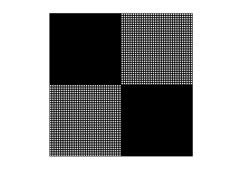
Figure 1: Representative volume element for a checkerboard composite.

The phase interchange identity [5] for the effective shear modulus of a symmetric two-dimensional two-component isotropic composite is a duality-based exact relation that states that

$$G_{\text{eff}}=\sqrt{G_{1}G_{2}}$$ (1)

where $G_{1}$, $G_{2}$ are the shear moduli of the two components and $G_{\text{eff}}$ is the effective shear modulus.

The phase interchange identity is valid only for isotropic composites. In a finite-sized representative volume element (RVE) for a checkerboard composite the shear modulus is not the same all directions and hence isotropy is not achieved. The two-dimensional stress-strain relation for such a RVE with “square symmetry” can be written as

$$\left[\begin{array}[]{c}\sigma_{11}\\ \sigma_{22}\\ \sigma_{12}\end{array}\right]=\left[\begin{array}[]{lll}K+\mu^{1}&K-\mu^{1}&0\\ K-\mu^{1}&K+\mu^{1}&0\\ 0&0&\mu^{2}\end{array}\right]\left[\begin{array}[]{c}\epsilon_{11}\\ \epsilon_{22}\\ 2\left<\epsilon_{12}\right>_{\text{V}}\end{array}\right]$$ (2)

where $\sigma_{11}$, $\sigma_{22}$, $\sigma_{12}$ are the stresses; $\epsilon_{11}$, $\epsilon_{22}$, $\epsilon_{12}$ are the strains; $K$ is the two-dimensional bulk modulus, $\mu^{1}$ is the shear modulus when shear is applied along the diagonals of the RVE, and $\mu^{2}$ is the shear modulus for shear along the edges of the RVE.

The numerical verification of the phase interchange identity, therefore, requires that the components of the composite be chosen so that the difference between $\mu^{1}$ and $\mu^{2}$ for the composite is minimal. This implies that the components should have a weak modulus contrast.

Numerical estimates of the effective elastic properties of the checkerboard composite shown in Figure 1 were obtained using finite elements (FEM), the recursive cell method (RCM) and the generalized method of cells (GMC). Following the requirement of low modulus contrast, both components were assigned a Young’s modulus of 15,300 MPa. The Poisson’s ratio of the first component was fixed at 0.32 while that of the second component was varied from 0.1 to 0.49. The FEM calculations were performed using a mesh of 256$\times$256 four-noded square elements. The RCM calculations used a grid of 64$\times$64 subcells with blocks of 2$\times$2 subcells and each subcell was modeled using one nine-noded element. The GMC calculations used 64$\times$64 square subcells to discretize the RVE.

Figure 2 shows a comparison of the exact effective shear modulus for the checkerboard composite with estimates of $\mu^{1}$ and $\mu^{2}$ from the three numerical approaches.

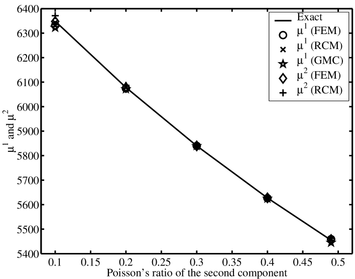
Figure 2: Validation of FEM, RCM and GMC using the phase interchange identity for a checkerboard composite.

The results show that all the three methods perform well (the maximum error is 0.1%) in predicting the effective shear modulus when the modulus contrast is small, i.e., when the composite is nearly isotropic. It can also be observed that the values of $\mu^{1}$ and $\mu^{2}$ are within 1% of each other for the chosen component moduli.

2.1 Range of applicability

The question that arises at this point is whether the three numerical approaches can predict the phase interchange identity for larger modulus contrasts. Numerical calculations have been performed on the checkerboard microstructure to explore this issue. The first component of the checkerboard was assigned a Young’s modulus of 15,300 MPa and a Poisson’s ratio of 0.32. For the second component, the Poisson’s ratio was fixed at 0.49 and the Young’s modulus was varied from 0.7 MPa to 7000 MPa.

Figure 3 shows plots of the effective $\mu^{1}$ and $\mu^{2}$ versus shear modulus contrast for a checkerboard RVE.

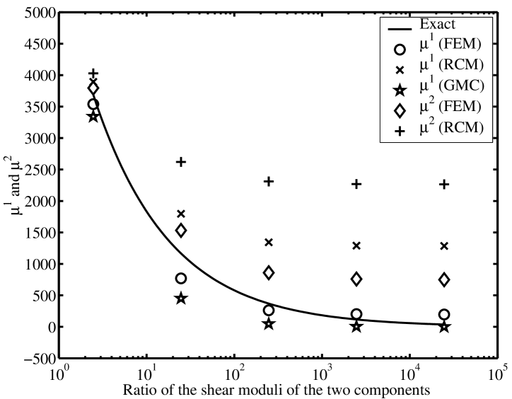
Figure 3: Variation of effective shear moduli with modulus contrast for a checkerboard composite.

The plots confirm that when the modulus contrast between the components of the checkerboard exceeds 2, the material can no longer be considered isotropic since the values of $\mu^{1}$ and $\mu^{2}$ are considerably different from each other. However, the values of $\mu^{1}$ predicted by FEM are quite close to the effective shear modulus $G_{\text{eff}}$ predicted by the phase interchange identity. This result suggests that the simulation of a diagonal shear may not be necessary to predict the effective shear modulus of an isotropic composite when the finite element approach is used. It also implies that the phase interchange identity can be used for a much larger range of modulus contrasts. The effective shear moduli predicted by GMC are considerably lower than that from the exact relation while the values from RCM are consistently higher. The RCM estimates worsen with increasing modulus contrast. If only the value of $\mu^{1}$ is examined, the phase interchange identity indicates that the FEM approach is much more accurate than the GMC and RCM approaches. However, it is difficult to choose between GMC and RCM for high modulus contrasts composites. While the exact value of $\mu^{1}$ is 10 times the value predicted by GMC, the corresponding RCM estimate is 10 times the exact value. These results confirm the findings of detailed numerical studies on high modulus contrast, high volume fraction polymer bonded explosives [8, 9, 4].

2.2 Convergence of FEM calculations

The checkerboard material provides an extreme case to test the convergence of the FEM solution because the corner singularities lead to high stresses that can only be resolved with refined meshes. Figure 4 shows the convergence of the effective $\mu^{1}$ and $\mu^{2}$ with increasing mesh refinement for a checkerboard with a shear modulus contrast of about 25,000.

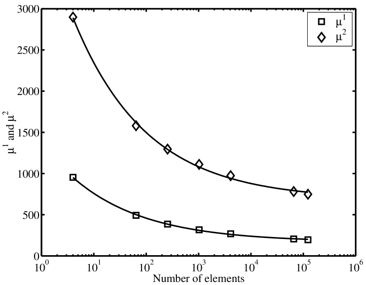
Figure 4: Convergence of effective moduli predicted by FEM with increase in mesh refinement for a checkerboard composite with a shear modulus contrast of 25,000.

The effective $\mu^{1}$ converges to a steady value when 128$\times$128 elements are used to discretize the RVE. The shear modulus $\mu^{2}$ reaches a steady value when 256$\times$256 elements are used. This is why the finite element calculations in this work were performed using 256$\times$256 elements or more.

RCM uses a finite element approach to homogenize blocks of subcells. When blocks of 2$\times$2 subcells are used, some of these blocks can resemble checkerboards - especially at the first level of recursion for a two-component composite. The finite element convergence result suggests that RCM may overestimate the effective shear moduli by a factor of two if a block of four subcells is simulated using only four finite elements.

3 Materials rigid in shear

The stress-strain response of two-dimensional materials that are rigid with respect to shear can be represented by

$$\left[\begin{array}[]{c}\epsilon_{11}\\ \epsilon_{22}\\ \epsilon_{12}\end{array}\right]=\left[\begin{array}[]{ccc}S_{11}&S_{12}&0\\ S_{12}&S_{22}&0\\ 0&0&0\end{array}\right]\left[\begin{array}[]{c}\sigma_{11}\\ \sigma_{22}\\ \sigma_{12}\end{array}\right]$$ (3)

where $\sigma_{11}$, $\sigma_{22}$, $\sigma_{12}$ are the stresses; $\epsilon_{11}$, $\epsilon_{22}$ and $\epsilon_{12}$ are the strains, and $S_{ij}$ are the components of the compliance matrix.

Two duality-based exact relations that are valid for two-component composites composed of such materials are [1]:

Relation RS1

If $S_{11}S_{22}-(S_{12})^{2}=\Delta$ for each phase (where $\Delta$ is a constant), then the effective compliance tensor also satisfies the same relationship, i.e., $S^{\text{eff}}_{11}S^{\text{eff}}_{22}-(S^{\text{eff}}_{12})^{2}=\Delta_{\text{eff}}$. This relation is true for all microstructures.

Relation RS2

If the compliance tensors of the two phases are of the form $\mathbf{S}_{1}=\alpha_{1}\mathbf{A}$ and $\mathbf{S}_{2}=\alpha_{2}\mathbf{A}$ where $\mathbf{A}$ is a constant matrix, then the effective compliance tensor of a checkerboard of the two phases satisfies the relation $\det{\mathbf{S}_{\text{eff}}}=S^{\text{eff}}_{11}S^{\text{eff}}_{22}-(S^{\text{eff}}_{12})^{2}=\alpha_{1}\alpha_{2}(A_{11}A_{22}-(A_{12})^{2})$.

3.1 Relation RS1

Figure 5 shows a square array of disks occupying an area fraction of 0.7.

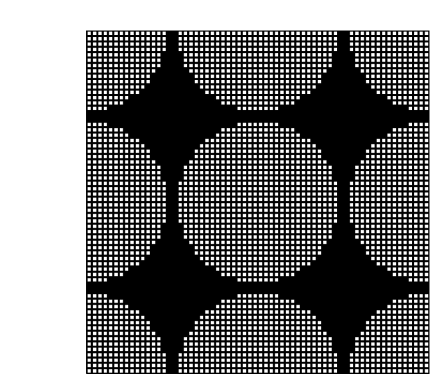
Figure 5: RVE for a square array of disks.

Numerical experiments have been performed on this array of disks to check if Relation RS1 can be reproduced by finite element analyses, GMC and RCM. The $\mathbf{S}$ matrices that have been used for the disks (superscript $1$) and the matrix (superscript $2$), and the corresponding values of $\Delta$ are shown below. These matrices have been chosen so that the value of $\Delta$ is constant.

$$\mathbf{S}_{1}=\left[\begin{array}[]{ccc}1000&-300&0\\ -300&1000&0\\ 0&0&0.001\end{array}\right],~{}\Delta=9.1\times 10^{5},$$

and

$$\mathbf{S}_{2}=\left[\begin{array}[]{ccc}1094.3&-536.21&0\\ -536.21&1094.3&0\\ 0&0&0.001\end{array}\right],~{}\Delta=9.1\times 10^{5}.$$

The shear modulus for both materials is $1000$ (arbitrary units) - around $10^{6}$ times the Young’s modulus. Higher values of shear modulus have been tested and found not to affect the effective stiffness matrix significantly.

Table 1 shows the values of $S^{\text{eff}}_{11}$, $S^{\text{eff}}_{12}$ and $\Delta_{\text{eff}}$ calculated using finite elements (350$\times$350 elements), GMC (64$\times$64 subcells) and RCM (256$\times$256 subcells).

Table 1: Two-dimensional effective compliance matrix for a square array of disks.

	$S^{\text{eff}}_{11}$	$S^{\text{eff}}_{12}$	$\Delta_{\text{eff}}$ $(\times 10^{5})$	$\Delta_{\text{eff}}$/$\Delta$
FEM	850.35	-536.32	4.35	0.48
RCM	847.25	-538.17	4.28	0.47
GMC	871.75	-517.14	4.93	0.54

The ratio of the calculated $\Delta_{\text{eff}}$ to the original $\Delta$ are also shown in the table. The modulus contrast between the two components of the composite is small, so the calculated effective properties are expected to be accurate (based on the results on the phase interchange identity for shear moduli). However, the results in Table 1 show that all the three numerical methods predict values of $\Delta_{\text{eff}}$ that are around half the original $\Delta$. These results imply that all three methods (FEM, GMC and RCM) overestimate the effective normal stiffness of the array of disks. Relation RS1 for materials rigid in shear may therefore be a very sensitive test of the accuracy of numerical methods even though the modulus contrast that can be used is small.

3.2 Relation RS2

The second duality relation for materials that are rigid in shear requires (Relation RS2) is valid for the checkerboard geometry shown in Figure 1. The following values of the elastic properties have been used to test the accuracy of FEM, RCM and GMC in predicting this relation.

$$\mathbf{S}_{1} =100\left[\begin{array}[]{cc}10&-3\\ -3&10\end{array}\right]~{};~{}\mathbf{S}_{2}=1000\left[\begin{array}[]{cc}10&-3\\ -3&10\end{array}\right]$$

$$\alpha_{1} =100~{};~{}\alpha_{2}=1000$$

$$\mathbf{A} =\left[\begin{array}[]{cc}10&-3\\ -3&10\end{array}\right]$$

The duality relation requires that the effective compliance matrix of the checkerboard composite should be such that

$$\det(\mathbf{S}_{\text{eff}})=S^{\text{eff}}_{11}S^{\text{eff}}_{22}-(S^{\text{eff}}_{12})^{2}=9.10\times 10^{6}~{}.$$

The FEM calculations were performed using 350$\times$350 four-noded elements, the RCM calculations used 64$\times$64 subcells (blocks of 2$\times$2 subcells) and the GMC calculations used 64$\times$64 subcells too. The results from these three methods are tabulated in Table 2.

Table 2: Effective compliance matrix for a checkerboard composite with components rigid in shear.

	$S^{\text{eff}}_{11}$	$S^{\text{eff}}_{12}$	$\det(\mathbf{S}_{\text{eff}})(\times 10^{6})$	$\det(\mathbf{S}^{\text{eff}})/\alpha_{1}\alpha_{2}\det{\mathbf{A}}$
FEM	3282	-2004	6.75	0.74
RCM	1655	-7090	2.23	0.24
GMC	5007	-2146	2.05	2.25

The finite element calculations lead to quite an accurate effective compliance matrix and the deviation from the exact result is only around 25%. The GMC calculations overestimate the compliance matrix and the determinant of the compliance matrix is around 2.3 times higher than the exact result. On the other hand, the RCM calculations predict a compliance matrix that has a determinant that is only around 20

4 The CLM theorem

The Cherkaev, Lurie and Milton (CLM) theorem is a well known “translation” based exact relation for two-component planar composites [6]. For a two-dimensional two-component isotropic composite, this theorem can be stated as follows.

Let the isotropic bulk moduli of the components be $K_{1}$ and $K_{2}$. Let the shear moduli of the two components be $G_{1}$ and $G_{2}$. The effective bulk and shear modulus of a two-dimensional composite made of these two components are $K_{\text{eff}}$ and $G_{\text{eff}}$ respectively. Let us now create two new materials that are “translated” from the original component materials by a constant amount $\lambda$. That is, let the bulk and shear moduli of the translated component materials be given by

$$1/K^{T}_{1}=1/K_{1}-\lambda~{};~{}1/K^{T}_{2}=1/K_{2}-\lambda~{};$$

$$1/G^{T}_{1}=1/G_{1}+\lambda~{};~{}1/G^{T}_{2}=1/G_{2}+\lambda~{}.$$

The CLM theorem states that the effective bulk and shear moduli of a two-dimensional composite of the two translated materials, having the same microstructure as the original composite, are given by

$$1/K^{T}_{\text{eff}}=1/K_{\text{eff}}-\lambda~{};~{}1/G^{T}_{\text{eff}}=1/G_{\text{eff}}+\lambda.$$ (6)

The requirement of isotropy can be satisfied approximately by choosing component material properties that are close to each other. Since our goal is to determine how well GMC and RCM perform for high modulus contrast, choosing materials with small modulus contrast is not adequate. Another alternative is to choose a RVE that represents a hexagonal packing of disks. However, such an RVE is necessarily rectangular and cannot be modeled using RCM in its current form. It should be noted that RCM can easily be modified to deal with elements that are not square and hence to model rectangular regions.

Another problem in the application of the CLM theorem is that the value of $\lambda$ has to be small if the difference between the original and the translated moduli is large and vice versa. If the value of $\lambda$ is small, floating point errors can accumulate and exceed the value of $\lambda$. On the other hand, if $\lambda$ is large, the original and the translated moduli are very close to each other and the difference between the two can be lost because of errors in precision. Hence, the numbers have to be chosen carefully keeping in mind the limits on the value of the Poisson’s ratio.

The translation relation has been tested on the square array of disks occupying a volume fraction of 0.70 from Figure 5. This RVE exhibits square symmetry, i.e., the shear moduli $\mu^{1}$ and $\mu^{2}$ shown in equation (2) are not equal. A unique value of the effective shear modulus cannot be calculated for this RVE. Instead, he value of the effective translated shear modulus is calculated from equation (6) by first setting $G_{\text{eff}}$ equal to $\mu^{1}$ and then to $\mu^{2}$. These “exact” values are compared with the $\mu^{1}$ and $\mu^{2}$ values predicted using finite element analyses, GMC and RCM.

The original set of elastic moduli for the RVE is chosen to reflect the elastic moduli of the constituents of polymer bonded explosives. These moduli are then translated by a constant $\lambda=0.001$. The original and the translated constituent two-dimensional moduli are shown in Table 3 (phase ’p’ represents the particles and phase ’b’ represents the binder). It can be observed that the translation process creates quite a large change in the bulk modulus of the particles.

Table 3: Original and translated two-dimensional constituent moduli for checking the CLM condition.

	$K_{p}$	$G_{p}$	$K_{b}$	$G_{b}$	$K_{p}/K_{b}$	$G_{p}/G_{b}$
	$(\times 10^{2})$	$(\times 10^{2})$			$(\times 10^{2})$	$(\times 10^{2})$
Original	9.60	4.80	10.07	0.20	0.95	23.8
Translated	240.0	3.24	10.17	0.20	23.5	16.1

Table 4 shows the effective bulk and shear moduli of the original and the translated material calculated using finite elements (350$\times$350 elements), GMC (64$\times$64 subcells) and RCM (256$\times$256 subcells). The values of $\lambda_{\text{err}}$ shown in the table have been calculated using the equation

$$\lambda_{\text{err}} =(\lambda/0.001-1)\times 100,$$

$$\lambda=1/K_{\text{eff}}-1/K^{T}_{\text{eff}}=1/\mu^{i(T)}_{\text{eff}}-1/\mu^{i}_{\text{eff}}.$$

Table 4: Comparison of effective moduli for the original and the translated composites.

	$K_{\text{eff}}$			$\mu^{1}_{\text{eff}}$			$\mu^{2}_{\text{eff}}$
	Orig.	Trans.	$\lambda_{\text{err}}$(%)	Orig.	Trans.	$\lambda_{\text{err}}$(%)	Orig.	Trans.	$\lambda_{\text{err}}$(%)
FEM	36.4	37.8	-0.8	10.1	10	-3.1	0.9	0.9	22
RCM	42.5	44.5	6.1	29.8	29	-6.9	1.3	1.3	-292
GMC	34.0	35.1	-1.3	3.8	3.8	5.3	0.7	0.7	30

Even though the modulus contrast between the two components of the composite is high, the effective properties predicted by FEM, GMC and RCM are close to each other in magnitude. The effective moduli of the translated composite are also quite close to that of the original composite as predicted by the CLM condition. The interesting fact is that all the three methods satisfy the CLM condition and the error is small (as seen by the values of $\lambda_{\text{err}}$. Of the three methods, FEM and GMC produce the least error while RCM produces the most error.

5 Composites with equal bulk modulus

The translation procedure can also be used to generate an exact solution for the effective shear modulus of two-dimensional symmetric two-component composites with both components having the same bulk modulus [5]. This relation is

$$K_{\text{eff}} =~{}K~{}=~{}K_{1}~{}=~{}K_{2}$$

$$G_{\text{eff}} =\frac{K}{-1+\sqrt{\left(1+\frac{K}{G_{1}}\right).\left(1+\frac{K}{G_{2}}\right)}}$$ (7)

This relation has been tested on the checkerboard model shown in Figure 1 using the component material properties given in Table 5. The exact effective properties for the composite, calculated using equation (7), are also given in the table. The values of the effective moduli calculated using finite elements (FEM), GMC and RCM are also shown in Table 5.

Table 5: Component properties, exact effective properties and numerically computed effective properties for two-component symmetric composite with equal component bulk moduli.

	$E$	$\nu$	$K$	$G$
	$(\times 10^{2})$		$(\times 10^{3})$	$(\times 10^{2})$
Component 1	25.00	0.25	2.0	10.0
Component 2	1.19	0.49	2.0	0.4
Composite	5.12	0.46	2.0	1.76

	$K_{\text{eff}}$	$\mu^{1}_{\text{eff}}$	Diff.	$\mu^{2}_{\text{eff}}$	Diff.
	$(\times 10^{2})$	$(\times 10^{2})$	%	$(\times 10^{2})$	%
FEM	20	1.29	-26.8	2.54	44.4
GMC	20	0.77	-56.3	0.77	-56.3
RCM	20	2.96	68.0	4.41	150.9

These results show that the effective two-dimensional bulk modulus is calculated correctly by all the three methods. However, the shear moduli calculated for the checkerboard microstructure are quite different from the exact result. This exact result also shows that the FEM calculations are the most accurate, followed by GMC and then RCM. The values of $\mu^{1}_{\text{eff}}$ are also found to most closely approximate the value of $G_{\text{eff}}$.

6 Hill’s equation

Hill’s equation [7] is an exact relation that is independent of microstructure. This equation is valid for composites composed of isotropic components that have the same shear modulus. For a two-dimensional two-component composite, this equation can be written as

$$\frac{1}{K_{\text{eff}}+G}=\frac{f_{p}}{K_{p}+G}+\frac{f_{b}}{K_{b}+G}$$ (8)

where $f$ represents a volume fraction, $K$ represents a bulk modulus, and $G$ represents a shear modulus. The subscript ’$p$’ represents a particle property, ’$b$’ represents a binder property, and ’eff’ represents the effective property of the composite.

This relationship is verified using the RVE containing an array of disks occupying 70% of the volume that is shown in Figure 5. Table 6 shows the properties of the two components used to compare the predictions of finite elements, GMC and RCM with the exact value of bulk modulus predicted by Hill’s equation. It should be noted that the materials chosen are not quite representative of polymer bonded explosive materials.

Table 6: Phase properties used for testing Hill’s equation and the exact effective moduli of the composite.

	Vol.	$E$	$\nu$	$G$	$K$
	Frac.	$(\times 10^{3})$		$(\times 10^{3})$	$(\times 10^{3})$
Disks	0.7	3.00	0.25	1.20	2.40
Binder	0.3	3.58	0.49	1.20	60.00
Composite	1.0	3.22	0.34	1.20	3.82

Since the modulus contrast is small, the square array of disks is expected to exhibit nearly isotropic behavior. Therefore, the predictions of finite elements, GMC and RCM are expected to be close to the exact values of the effective properties of the composite. The numerically calculated values of the effective two-dimensional bulk and shear moduli of the composite are shown in Table 7. The percentage difference of the effective bulk modulus from the exact value is also shown in the table.

Table 7: Numerically computed effective properties for a square array of disks with equal component shear moduli.

	$K_{\text{eff}}$	% Diff.	$\mu^{1}_{\text{eff}}$	$\mu^{2}_{\text{eff}}$
	($\times 10^{3}$)		($\times 10^{3}$)	($\times 10^{3}$)
FEM	3.98	4.4	1.20	1.20
RCM	3.92	2.7	1.20	1.20
GMC	3.66	-4.2	1.20	1.20

The effective shear moduli predicted by all the three methods are exact. In case of the effective bulk moduli, the RCM predictions are the most accurate followed by GMC and the finite element based calculations. The finite element based calculations overestimate the effective two-dimensional bulk modulus by around 4.4% while GMC underestimates the bulk modulus by around 4.2%. Since the error of estimation of all the three methods is small, it is suggested that all three methods are accurate for low contrasts in the shear modulus. However, Hill’s equation does not appear to be suitable for determining the best numerical method of the three.

7 Summary and conclusions

Predictions from the phase interchange identity for the shear modulus are closely approximated by the finite element approach (FEM), the recursive cell method (RCM) and the generalized method of cells (GMC) for checkerboard composites with low modulus contrast. However, for higher modulus contrasts the FEM approximations of shear moduli are the most accurate. The RCM predictions overestimate the shear modulus while GMC underestimates the shear modulus. The exact relations for materials that are rigid in shear show that all three numerical techniques are inaccurate. The exact relation for this class of materials that is applicable to checkerboard materials shows that the FEM calculations are the most accurate while both RCM and GMC perform poorly in comparison. Though the predictions of the CLM theorem are quite accurately predicted by all three numerical methods for high modulus contrast composites, the FEM results show the least error between the original and the translated effective properties while the RCM results show the largest error. The exact relation for isotropic composites with components that have the same bulk moduli also shows that the FEM predictions are the most accurate though they are somewhat higher than the exact values. However, no such distinction between the three methods can be made using Hill’s equation. These results reflect previous studies for high modulus contrast, high volume fraction polymer bonded explosives using FEM, RCM and RCM and show that exact relations can be used to determine the accuracy of numerical methods without performing detailed numerical studies.

Appendix

The components of the two-dimensional stiffness matrix can be computed from two-dimensional plane strain finite element analyses. However, the components of the two-dimensional compliance matrix cannot be directly determined from two-dimensional plane strain finite element analyses. The reasons for these are discussed in this appendix. The approach taken to approximate the two-dimensional compliance matrix is also discussed.

A.1 Two-Dimensional Stiffness Matrix

The stress-strain relation for an anisotropic linear elastic material is given by

$$\left[\begin{array}[]{c}\sigma_{11}\\ \sigma_{22}\\ \sigma_{33}\\ \sigma_{23}\\ \sigma_{31}\\ \sigma_{12}\end{array}\right]=\left[\begin{array}[]{cccccc}C_{11}&C_{12}&C_{13}&C_{14}&C_{15}&C_{16}\\ C_{12}&C_{22}&C_{23}&C_{24}&C_{25}&C_{26}\\ C_{13}&C_{23}&C_{33}&C_{34}&C_{35}&C_{36}\\ C_{14}&C_{24}&C_{34}&C_{44}&C_{45}&C_{46}\\ C_{15}&C_{25}&C_{35}&C_{45}&C_{55}&C_{56}\\ C_{16}&C_{26}&C_{36}&C_{46}&C_{56}&C_{66}\end{array}\right]\left[\begin{array}[]{c}\epsilon_{11}\\ \epsilon_{22}\\ \epsilon_{33}\\ \epsilon_{23}\\ \epsilon_{31}\\ \epsilon_{12}\end{array}\right].$$ (9)

For the plane strain assumption, we have,

$$\epsilon_{33}~{}=~{}\epsilon_{23}~{}=~{}\epsilon_{31}~{}=~{}0.$$ (10)

Therefore, the stress-strain relation can be reduced to

$$\left[\begin{array}[]{c}\sigma_{11}\\ \sigma_{22}\\ \sigma_{12}\end{array}\right]=\left[\begin{array}[]{ccc}C_{11}&C_{12}&C_{16}\\ C_{12}&C_{22}&C_{26}\\ C_{16}&C_{26}&C_{66}\end{array}\right]\left[\begin{array}[]{c}\epsilon_{11}\\ \epsilon_{22}\\ \epsilon_{12}\end{array}\right].$$ (11)

The six terms in the apparent two-dimensional stiffness matrix reduce to four is the material is orthotropic, i.e.,

$$\left[\begin{array}[]{c}\sigma_{11}\\ \sigma_{22}\\ \sigma_{12}\end{array}\right]=\left[\begin{array}[]{ccc}C_{11}&C_{12}&0\\ C_{12}&C_{22}&0\\ 0&0&C_{66}\end{array}\right]\left[\begin{array}[]{c}\epsilon_{11}\\ \epsilon_{22}\\ \epsilon_{12}\end{array}\right].$$ (12)

The three constants $C_{11}$, $C_{12}$ and $C_{22}$ can be determined by the application of normal displacements in the ’1’ and ’2’ directions respectively. The constant $C_{66}$ can be determined using shear displacement boundary conditions in a finite element analysis. Hence, it can be seen that the stiffness matrix can be calculated directly from two-dimensional plane strain based finite element analyses. This is not true for the compliance matrix.

A.2 Two-Dimensional Compliance Matrix

The strain-stress relation for an anisotropic linear elastic material can be written as

$$\left[\begin{array}[]{c}\epsilon_{11}\\ \epsilon_{22}\\ \epsilon_{33}\\ \epsilon_{23}\\ \epsilon_{31}\\ \epsilon_{12}\end{array}\right]=\left[\begin{array}[]{cccccc}S_{11}&S_{12}&S_{13}&S_{14}&S_{15}&S_{16}\\ S_{12}&S_{22}&S_{23}&S_{24}&S_{25}&S_{26}\\ S_{13}&S_{23}&S_{33}&S_{34}&S_{35}&S_{36}\\ S_{14}&S_{24}&S_{34}&S_{44}&S_{45}&S_{46}\\ S_{15}&S_{25}&S_{35}&S_{45}&S_{55}&S_{56}\\ S_{16}&S_{26}&S_{36}&S_{46}&S_{56}&S_{66}\end{array}\right]\left[\begin{array}[]{c}\sigma_{11}\\ \sigma_{22}\\ \sigma_{33}\\ \sigma_{23}\\ \sigma_{31}\\ \sigma_{12}\end{array}\right].$$ (13)

The relationship between the stiffness matrix and the compliance matrix is

$$\left[\begin{array}[]{cccccc}S_{11}&S_{12}&S_{13}&S_{14}&S_{15}&S_{16}\\ S_{12}&S_{22}&S_{23}&S_{24}&S_{25}&S_{26}\\ S_{13}&S_{23}&S_{33}&S_{34}&S_{35}&S_{36}\\ S_{14}&S_{24}&S_{34}&S_{44}&S_{45}&S_{46}\\ S_{15}&S_{25}&S_{35}&S_{45}&S_{55}&S_{56}\\ S_{16}&S_{26}&S_{36}&S_{46}&S_{56}&S_{66}\end{array}\right]=\left[\begin{array}[]{cccccc}C_{11}&C_{12}&C_{13}&C_{14}&C_{15}&C_{16}\\ C_{12}&C_{22}&C_{23}&C_{24}&C_{25}&C_{26}\\ C_{13}&C_{23}&C_{33}&C_{34}&C_{35}&C_{36}\\ C_{14}&C_{24}&C_{34}&C_{44}&C_{45}&C_{46}\\ C_{15}&C_{25}&C_{35}&C_{45}&C_{55}&C_{56}\\ C_{16}&C_{26}&C_{36}&C_{46}&C_{56}&C_{66}\end{array}\right]^{-1}$$ (14)

or,

$$\mathbf{S}=\mathbf{C}^{-1}.$$ (15)

It is obvious from the above equation that the apparent two-dimensional compliance matrix is not equal to the inverse of the apparent two-dimensional stiffness matrix, i.e.,

$$\left[\begin{array}[]{ccc}S_{11}&S_{12}&S_{16}\\ S_{12}&S_{22}&S_{26}\\ S_{16}&S_{26}&S_{66}\end{array}\right]\neq\left[\begin{array}[]{ccc}C_{11}&C_{12}&C_{16}\\ C_{12}&C_{22}&C_{26}\\ C_{16}&C_{16}&C_{66}\end{array}\right]^{-1}.$$ (16)

Hence, we cannot determine the two-dimensional compliance matrix if we only know the two-dimensional stiffness matrix.

Let us again examine the effect of the plane-strain assumption on the stress-strain relation. We then have

$$\left[\begin{array}[]{c}\epsilon_{11}\\ \epsilon_{22}\\ 0\\ \epsilon_{12}\end{array}\right]=\left[\begin{array}[]{cccc}S_{11}&S_{12}&S_{13}&S_{16}\\ S_{12}&S_{22}&S_{23}&S_{26}\\ S_{13}&S_{23}&S_{33}&S_{36}\\ S_{16}&S_{26}&S_{36}&S_{66}\end{array}\right]\left[\begin{array}[]{c}\sigma_{11}\\ \sigma_{22}\\ \sigma_{33}\\ \sigma_{12}\end{array}\right].$$ (17)

For orthotropic materials, this relation simplifies to

$$\left[\begin{array}[]{c}\epsilon_{11}\\ \epsilon_{22}\\ 0\\ \epsilon_{12}\end{array}\right]=\left[\begin{array}[]{cccc}S_{11}&S_{12}&S_{13}&0\\ S_{12}&S_{22}&S_{23}&0\\ S_{13}&S_{23}&S_{33}&0\\ 0&0&0&S_{66}\end{array}\right]\left[\begin{array}[]{c}\sigma_{11}\\ \sigma_{22}\\ \sigma_{33}\\ \sigma_{12}\end{array}\right].$$ (18)

This equation shows that we need to know the stress $\sigma_{33}$ to determine the terms of the compliance matrix and hence three-dimensional analyses are necessary. If we assume plane stress, we can determine the terms of the matrix $\mathbf{S}$ directly. However, the apparent two-dimensional compliance matrix for plane stress is not equal to that for plane strain and hence we cannot apply this method for our purposes. This is why the plane strain compliance matrix cannot be determined using two-dimensional finite element analyses only.

A.3 Approximation of Compliance Matrix

The two-dimensional compliance matrix can be determined approximately for materials with square symmetry by assuming that $S_{13}$, $S_{23}$ and $S_{33}$ are known. Let,

$$S_{13}=S_{23}=-\frac{\nu_{3}}{E_{3}}\\ S_{33}=\frac{1}{E_{3}}$$ (19)

where, $\nu_{3}$ is the Poisson’s ratio in the out-of-plane direction and $E_{3}$ is the Young’s ratio in that direction. Then, for a material with square symmetry,

$$\left[\begin{array}[]{c}\epsilon_{11}\\ \epsilon_{22}\\ 0\\ \epsilon_{12}\end{array}\right]=\left[\begin{array}[]{cccc}S_{11}&S_{12}&-\frac{\nu_{3}}{E_{3}}&0\\ S_{12}&S_{11}&-\frac{\nu_{3}}{E_{3}}&0\\ -\frac{\nu_{3}}{E_{3}}&-\frac{\nu_{3}}{E_{3}}&\frac{1}{E_{3}}&0\\ 0&0&0&S_{66}\end{array}\right]\left[\begin{array}[]{c}\sigma_{11}\\ \sigma_{22}\\ \sigma_{33}\\ \sigma_{12}\end{array}\right].$$ (20)

Inverting the relation, we have,

$$\left[\begin{array}[]{c}\sigma_{11}\\ \sigma_{22}\\ \sigma_{33}\\ \sigma_{12}\end{array}\right]=\left[\begin{array}[]{cccc}C_{11}&C_{12}&C_{13}&0\\ C_{12}&C_{11}&C_{23}&0\\ C_{13}&C_{23}&C_{33}&0\\ 0&0&0&C_{66}\end{array}\right]\left[\begin{array}[]{c}\epsilon_{11}\\ \epsilon_{22}\\ 0\\ \epsilon_{12}\end{array}\right].$$ (21)

where, $$C_{11}=\frac{E_{3}S_{11}-\nu_{3}^{2}}{E_{3}S_{11}^{2}-2\nu_{3}^{2}S_{11}-E_{3}S_{12}^{2}+2\nu^{2}S_{12}}~{},$$

$$C_{12}=\frac{-E_{3}S_{12}+\nu_{3}^{2}}{E_{3}S_{11}^{2}-2\nu_{3}^{2}S_{11}-E_{3}S_{12}^{2}+2\nu^{2}S_{12}}.$$

Note that it is not necessary to know $C_{13}$, $C_{23}$ and $C_{33}$ to determine $S_{11}$ and $S_{12}$.

We can write the above relations between $C_{11},C_{12}$ and $S_{11},S_{12}$ in the form

$$E_{3}S_{11}^{2}-\left(\frac{E_{3}}{C_{11}}+2\nu_{3}^{2}\right)S_{11}-\left(E_{3}S_{12}^{2}-2\nu_{3}^{2}S_{12}-\frac{\nu_{3}^{2}}{C_{11}}\right) =0,$$ (22)

$$E_{3}S_{12}^{2}-\left(\frac{E_{3}}{C_{12}}+2\nu_{3}^{2}\right)S_{12}-\left(E_{3}S_{11}^{2}-2\nu_{3}^{2}S_{11}+\frac{\nu_{3}^{2}}{C_{12}}\right) =0.$$ (23)

In simplified form,

$$A_{1}S_{11}^{2}+B_{1}S_{11}+C_{1} =0,$$ (24)

$$A_{2}S_{12}^{2}+B_{2}S_{12}+C_{2} =0.$$ (25)

We can solve these quadratic equations to get expressions for $S_{11}$ and $S_{12}$ as

$$S_{11} =\frac{-B+\sqrt{B^{2}-4AC}}{2A},$$ (26)

$$S_{12} =\frac{-B-\sqrt{B^{2}-4AC}}{2A}.$$ (27)

Knowing $C_{11}$, $C_{12}$, $E_{3}$ and $\nu_{3}$ these two equations can be solved iteratively to determine $S_{11}$ and $S_{12}$. The values of $C_{11}$ and $C_{12}$ can be determined using the procedure outlined at the beginning of this section. It remains to be discussed how $E_{3}$ and $\nu_{3}$ are to be determined.

A.4 Determination of $E_{3}$ and $\nu_{3}$

Two methods can be used to determine the values of $E_{3}$ and $\nu_{3}$ for our calculations. The first method is to assume that the rule of mixtures is accurate enough to determine the effective properties in the ’3’ direction. Thus, if the volume fraction of the first component is $f_{1}$ and that of the second component is $f_{2}$, we have,

$$E_{3} =f_{1}E_{1}+f_{2}E_{2},$$ (28)

$$\nu_{3} =f_{1}\nu_{1}+f_{2}\nu_{2}.$$ (29)

where $E_{i}$ and $\nu_{i}$ are the Young’s modulus and the Poisson’s ratio of the $i$th component.

The other option is to use the values of $S_{13}$, $S_{23}$ and $S_{33}$ obtained from GMC since these are also quite accurate for the out of plane direction. Thus, we have,

$$E_{3} =\frac{1}{S_{33}^{\text{GMC}}},$$ (30)

$$\nu_{3} =-S_{13}^{\text{GMC}}E_{3}.$$ (31)

This is the procedure we have use to determine the effective compliance matrices discussed in this paper.

References

- [1] J. Helsing, G. W. Milton, and A. B. Movchan. Duality relations, correspondences, and numerical results for planar elastic composites. J. Mech. Phys. Solids, 45(4):565–590, 1997.
- [2] G. W. Milton. Composites : a myriad of microstructure independent relations. In T. Tatsumi, E. Watanabe, and T. Kambe, editors, Theoretical and Applied Mechanics (Proc. XIX International Congress of Theoretical and Applied Mechanics, Kyoto, 1996), pages 443–459. Elsevier, Amsterdam, 1997.
- [3] J. Aboudi. Micromechanical analysis of composites by the method of cells - update. Appl. Mech. Rev, 49(10):S83–S91, 1996.
- [4] B. Banerjee and D. O. Adams. On predicting the effective elastic properties of polymer bonded explosives using the recursive cell method. 2002.
- [5] G. W. Milton. Theory of Composites. Cambridge University Press, New York, 2002.
- [6] A. V. Cherkaev, K. A. Lurie, and G. W. Milton. Invariant properties of the stress in plane elasticity and equivalence classes of composites. Proc. R. Soc. Lond. A, 438(1904):519–529, 1992.
- [7] R. Hill. Theory of mechanical properties of fibre-strengthened materials: I. elastic behaviour. J. Mech. Phys. Solids, 12:199–212, 1964.
- [8] B. Banerjee and D. O. Adams. Effective elastic moduli of polymer bonded explosives from finite element simulations. 2002.
- [9] B. Banerjee and D. O. Adams. Application of the generalized method of cells to polymer bonded explosives. 2002.