MATERIAL POINT METHOD SIMULATIONS OF FRAGMENTING CYLINDERS

Abstract

Most research on the simulation of deformation and failure of metals has been and continues to be performed using the finite element method. However, the issues of mesh entanglement under large deformation, considerable complexity in handling contact, and difficulties encountered while solving large deformation fluid-structure interaction problems have led to the exploration of alternative approaches. The material point method uses Lagrangian solid particles embedded in an Eulerian grid. Particles interact via the grid with other particles in the same body, with other solid bodies, and with fluids. Thus, the three issues mentioned in the context of finite element analysis are circumvented.

In this paper, we present simulations of cylinders which fragment due to explosively expanding gases generated by reactions in a high energy material contained inside. The material point method is the numerical method chosen for these simulations discussed in this paper. The plastic deformation of metals is simulated using a hypoelastic-plastic stress update with radial return that assumes an additive decomposition of the rate of deformation tensor. Various plastic strain, plastic strain rate, and temperature dependent flow rules and yield conditions are investigated. Failure at individual material points is determined using porosity, damage and bifurcation conditions. Our models are validated using data from high strain rate impact experiments. It is concluded that the material point method possesses great potential for simulating high strain-rate, large deformation fluid-structure interaction problems.

Material Point Method, Fragmentation.

1 Introduction

The goal of this work is to present results from the simulation of the deformation and failure of a steel container that expands under the effect of gases produced by an explosively reacting high energy material (PBX 9501) contained inside.

The high energy material reacts at temperatures of 450 K and above, This elevated temperature is achieved through external heating of the steel container. Experiments conducted at the University of Utah have shown that failure of the container can be due to ductile fracture associated with void coalescence and adiabatic shear bands. If shear bands dominate the steel container fragments, otherwise a few large cracks propagate along the cylinder and pop it open.

Figure 1 shows the recovered parts of AISI 1026 steel containers after two different tests. The containers were initially 10 cm. in diameter and 0.6 cm thick. In the first test, shown in Figure 1(a), the container was heated over an open pool fire and shows ductile failure. In the second test, shown in Figure 1(b), the container was heated by means of electrical tape and fragmented after the explosion.

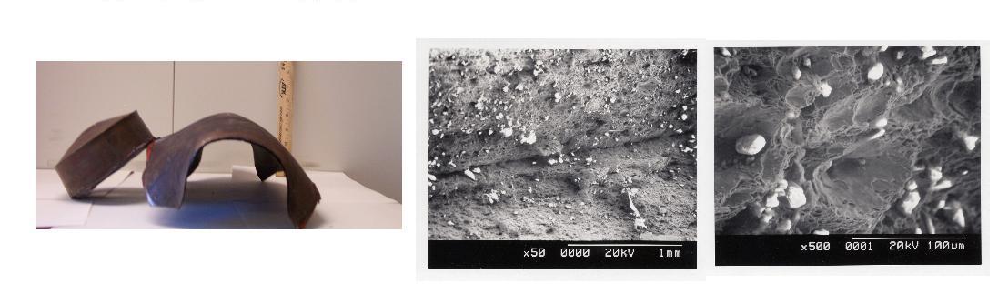
(a) Ductile fracture/Void Growth and Coalescence

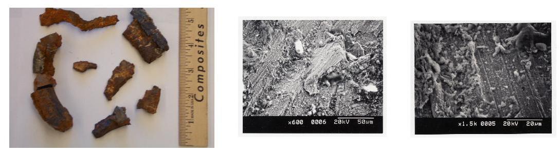
(b) Fragmentation/Adiabatic Shear Bands

Figure 1: Experimental tests of exploding cylinders.

The dynamics of the solid materials - steel and PBX 9501 - is modeled using the Lagrangian Material Point Method (MPM) [Sulsky et al. (1994)]. Gases are generated from solid PBX 9501 using a burn model [Long and Wight (2002)]. Gas-solid interaction is accomplished using an Implicit Continuous Eulerian (ICE) multi-material hydrodynamic code [Guilkey et al. (2004)]. A single computational grid is used for all the materials.

The constitutive response of PBX 9501 is modeled using ViscoSCRAM [Bennett et al. (1998)], which is a five element generalized Maxwell model for the viscoelastic response coupled with statistical crack mechanics. Solid PBX 9501 is progressively converted into a gas with an appropriate equation of state. The temperature and pressure in the gas increase rapidly as the reaction continues. As a result, the steel container is pressurized, undergoes plastic deformation, and finally fragments. The entire process was simulated using the massively parallel, Common Component Architecture  [Armstrong et al. (1999)] based, Uintah Computational Framework (UCF) [de St. Germain et al. (2000)].

The main issues regarding the constitutive modeling of the steel container are the selection of appropriate models for nonlinear elasticity, plasticity, damage, loss of material stability, and failure. The numerical simulation of the steel container involves the choice of appropriate algorithms for the integration of balance laws and constitutive equations, as well as the methodology for fracture simulation. Models and simulation methods for the steel container are required to be temperature sensitive and valid for large distortions, large rotations, and a range of strain rates (quasistatic at the beginning of the simulation to approximately $10^{6}$ s^-1 at fracture).

The approach chosen for the present work is to use hypoelastic-plastic constitutive models that assume an additive decomposition of the rate of deformation tensor into elastic and plastic parts. Hypoelastic materials are known not to conserve energy in a loading-unloading cycle unless a very small time step is used. However, the choice of this model is justified under the assumption that elastic strains are expected to be small for the problem under consideration and unlikely to affect the computation significantly.

Two plasticity models for flow stress are considered along with a two different yield conditions. Explicit fracture simulation is computationally expensive and prohibitive in the large simulations under consideration. The choice, therefore, has been to use damage models and stability criteria for the prediction of failure (at material points) and particle erosion for the simulation of fracture propagation.

The outline of the paper is as follows. A brief description of the Material Point Method is given in Section 2. The stress update algorithm and the how various plasticity models, yield conditions, equations of state etc. are used during the stress update are discussed in Section 3. The models used for the simulations are discussed in Section 4. The results of some simulations are presented in Section 5 and conclusions are presented in Section 6.

2 The Material Point Method

The Material Point Method (MPM)  [Sulsky et al. (1994)] is a particle method for structural mechanics simulations. In this method, the state variables of the material are described on Lagrangian particles or ”material points”. In addition, a regular, structured Eulerian grid is used as a computational scratch pad to compute spatial gradients and to solve the governing conservation equations. An explicit time-stepping version of the Material Point Method has been used in the simulations presented in this paper. The MPM algorithm is summarized below [Sulsky et al. (1995)].

It is assumed that an particle state at the beginning of a time step is known. The mass ($m$), external force ($\mathbf{f}^{\text{ext}}$), and velocity ($\mathbf{v}$) of the particles are interpolated to the grid using the relations

$$m_{g}=\sum_{p}S_{gp}~{}m_{p}~{},~{}~{}~{}~{}\mathbf{v}_{g}=(1/m_{g})\sum_{p}S_{gp}~{}m_{p}~{}\mathbf{v}_{p}~{},~{}~{}~{}~{}\mathbf{f}^{\text{ext}}_{g}=\sum_{p}S_{gp}~{}\mathbf{f}^{\text{ext}}_{p}$$ (1)

where the subscript ($g$) indicates a quantity at a grid node and a subscript ($p$) indicates a quantity on a particle. The symbol $\sum_{p}$ indicates a summation over all particles. The quantity ($S_{gp}$) is the interpolation function of node ($g$) evaluated at the position of particle ($p$). Details of the interpolants used can be found elsewhere [Bardenhagen and Kober (2004)].

Next, the velocity gradient at each particle is computed using the grid velocities using the relation

$$\boldsymbol{\nabla}\mathbf{v}_{p}=\sum_{g}\mathbf{G}_{gp}\mathbf{v}_{g}$$ (2)

where $\mathbf{G}_{gp}$ is the gradient of the shape function of node ($g$) evaluated at the position of particle ($p$). The velocity gradient at each particle is used to determine the Cauchy stress ($\boldsymbol{\sigma}_{p}$) at the particle using a stress update algorithm.

The internal force at the grid nodes ($\mathbf{f}^{\text{int}}_{g}$) is calculated from the divergence of the stress using

$$\mathbf{f}^{\text{int}}_{g}=\sum_{p}\mathbf{G}_{gp}~{}\boldsymbol{\sigma}_{p}~{}V_{p}$$ (3)

where $V_{p}$ is the particle volume.

The equation for the conservation of linear momentum is next solved on the grid. This equation can be cast in the form

$$\mathbf{m}_{g}~{}a_{g}=\mathbf{f}^{\text{ext}}_{g}-\mathbf{f}^{\text{int}}_{g}$$ (4)

where $\mathbf{a}_{g}$ is the acceleration vector at grid node ($g$).

The velocity vector at node ($g$) is updated using an explicit (forward Euler) time integration, and the particle velocity and position are then updated using grid quantities. The relevant equations are

$$\mathbf{v}_{g}(t+\Delta t) =\mathbf{v}_{g}(t)+\mathbf{a}_{g}~{}\Delta t$$ (5)

$$\mathbf{v}_{p}(t+\Delta t) =\mathbf{v}_{p}(t)+\sum_{g}S_{gp}~{}\mathbf{a}_{g}~{}\Delta t~{};~{}~{}~{}~{}\mathbf{x}_{p}(t+\Delta t)=\mathbf{x}_{p}(t)+\sum_{g}S_{gp}~{}\mathbf{v}_{g}~{}\Delta t$$ (6)

The above sequence of steps is repeated for each time step. The above algorithm leads to particularly simple mechanisms for handling contact. Details of these contact algorithms can be found elsewhere [Bardenhagen et al. (2001)].

3 Plasticity and Failure Simulation

A hypoelastic-plastic, semi-implicit approach [Zocher et al. (2000)] has been used for the stress update in the simulations presented in this paper. An additive decomposition of the rate of deformation tensor into elastic and plastic parts has been assumed. One advantage of this approach is that it can be used for both low and high strain rates. Another advantage is that many strain-rate and temperature-dependent plasticity and damage models are based on the assumption of additive decomposition of strain rates, making their implementation straightforward.

The stress update is performed in a co-rotational frame which is equivalent to using the Green-Naghdi objective stress rate. An incremental update of the rotation tensor is used instead of a direct polar decomposition of the deformation gradient. The accuracy of model is good if elastic strains are small compared to plastic strains and the material is not unloaded. It is also assumed that the stress tensor can be divided into a volumetric and a deviatoric component. The plasticity model is used to update only the deviatoric component of stress assuming isochoric behavior. The hydrostatic component of stress is updated using a solid equation of state.

Since the material in the container may unload locally after fracture, the hypoelastic-plastic stress update may not work accurately under certain circumstances. An improvement would be to use a hyperelastic-plastic stress update algorithm. Also, the plasticity models are temperature dependent. Hence there is the issue of severe mesh dependence due to change of the governing equations from hyperbolic to elliptic in the softening regime  [Hill and Hutchinson (1975), Bazant and Belytschko (1985), Tvergaard and Needleman (1990)]. Viscoplastic stress update models or nonlocal/gradient plasticity models [Ramaswamy and Aravas (1998a), Hao et al. (2000)] can be used to eliminate some of these effects and are currently under investigation.

A particle is tagged as ”failed” when its temperature is greater than the melting point of the material at the applied pressure. An additional condition for failure is when the porosity of a particle increases beyond a critical limit. A final condition for failure is when a bifurcation condition such as the Drucker stability postulate is satisfied. Upon failure, a particle is either removed from the computation by setting the stress to zero or is converted into a material with a different velocity field which interacts with the remaining particles via contact. Either approach leads to the simulation of a newly created surface.

In the parallel implementation of the stress update algorithm, sockets have been added to allow for the incorporation of a variety of plasticity, damage, yield, and bifurcation models without requiring any change in the stress update code. The algorithm is shown in Algorithm 1. The equation of state, plasticity model, yield condition, damage model, and the stability criterion are all polymorphic objects created using a factory idiom in C++ [Coplien (1992)].

Data: Persistent:Initial moduli, temperature, porosity, scalar damage, equation of state, plasticity model, yield condition, stability criterion, damage model

Temporary:Particle state at time $t$

Result: Particle state at time $t+\Delta t$

for all the patches in the domain do

       Read the particle data and initialize updated data storage;

       for all the particles in the patch do

             Compute the velocity gradient, the rate of deformation tensor and the spin tensor;

             Compute the updated left stretch tensor, rotation tensor, and deformation gradient;

             Rotate the input Cauchy stress and the rate of deformation tensor to the material configuration;

             Compute the current shear modulus and melting temperature;

             Compute the pressure using the equation of state, update the hydrostatic stress, and compute the trial deviatoric stress;

             Compute the flow stress using the plasticity model;

             Evaluate the yield function;

             if particle is elastic then

                   Rotate the stress back to laboratory coordinates;

                   Update the particle state;

                  

            else

                   Find derivatives of the yield function;

                   Do radial return adjustment of deviatoric stress;

                   Compute updated porosity, scalar damage, and temperature increase due to plastic work;

                   Compute elastic-plastic tangent modulus and evaluate stability condition;

                   Rotate the stress back to laboratory coordinates;

                   Update the particle state;

                   if Temperature $>$ Melt Temperature or Porosity $>$ Critical Porosity or Unstable then

                         Tag particle as failed;

                        

                   end if

                  

             end if

            

       end for

      

end for

Convert failed particles into a material with a different velocity field;

Algorithm 1 Stress Update Algorithm

4 Models

The stress in the solid is partitioned into a volumetric part and a deviatoric part. Only the deviatoric part of stress is used in the plasticity calculations assuming isoschoric plastic behavior.

The hydrostatic pressure ($p$) is calculated either using the bulk modulus ($K$) and shear modulus ($\mu$) or from a temperature-corrected Mie-Gruneisen equation of state of the form [Zocher et al. (2000)]

$$p=\frac{\rho_{0}C_{0}^{2}\zeta\left[1+\left(1-\frac{\Gamma_{0}}{2}\right)\zeta\right]}{\left[1-(S_{\alpha}-1)\zeta\right]^{2}+\Gamma_{0}C_{p}T}~{},~{}~{}~{}~{}\zeta=(\rho/\rho_{0}-1)$$ (7)

where $C_{0}$ is the bulk speed of sound, $\rho_{0}$ is the initial density, $\rho$ is the current density, $C_{p}$ is the specific heat at constant volume, $T$ is the temperature, $\Gamma_{0}$ is the Gruneisen’s gamma at reference state, and $S_{\alpha}$ is the linear Hugoniot slope coefficient.

Depending on the plasticity model being used, the pressure and temperature-dependent shear modulus ($\mu$) and the pressure-dependent melt temperature ($T_{m}$) are calculated using the relations [Steinberg et al. (1980)]

$$\mu =\mu_{0}\left[1+A\frac{p}{\eta^{1/3}}-B(T-300)\right]$$ (8)

$$T_{m} =T_{m0}\exp\left[2a\left(1-\frac{1}{\eta}\right)\right]\eta^{2(\Gamma_{0}-a-1/3)}$$ (9)

where, $\mu_{0}$ is the shear modulus at the reference state($T$ = 300 K, $p$ = 0, $\epsilon_{p}$ = 0), $\epsilon_{p}$ is the plastic strain. $\eta=\rho/\rho_{0}$ is the compression, $A=(1/\mu_{0})(d\mu/dp)$, $B=(1/\mu_{0})(d\mu/dT)$, $T_{m0}$ is the melt temperature at $\rho=\rho_{0}$, and $a$ is the coefficient of the first order volume correction to Gruneisen’s gamma.

We have explored two temperature and strain rate dependent plasticity models - the Johnson-Cook plasticity model [Johnson and Cook (1983)] and the Mechanical Threshold Stress (MTS) plasticity model [Follansbee and Kocks (1988), Goto et al. (2000)]. The flow stress ($\sigma_{f}$) from the Johnson-Cook model is given by

$$\sigma_{f}=[A+B(\epsilon_{p})^{n}][1+C\ln(\dot{\epsilon_{p}^{*}})][1-(T^{*})^{m}]~{};~{}~{}\dot{\epsilon_{p}^{*}}=\cfrac{\dot{\epsilon_{p}}}{\dot{\epsilon_{p0}}}~{};~{}~{}T^{*}=\cfrac{(T-T_{r})}{(T_{m}-T_{r})}$$ (10)

where $\dot{\epsilon_{p0}}$ is a user defined plastic strain rate, A, B, C, n, m are material constants, $T_{r}$ is the room temperature, and $T_{m}$ is the melt temperature.

The flow stress for the MTS model is given by

$$\sigma_{f}=\sigma_{a}+\frac{\mu}{\mu_{0}}S_{i}\hat{\sigma}_{i}+\frac{\mu}{\mu_{0}}S_{e}\hat{\sigma}_{e}$$ (11)

where

$$\mu =\mu_{0}-\frac{D}{\exp\left(\frac{T_{0}}{T}\right)-1}$$

$$S_{i} =\left[1-\left(\frac{kT}{g_{0i}\mu b^{3}}\ln\frac{\dot{\epsilon}_{0i}}{\dot{\epsilon}}\right)^{1/qi}\right]^{1/pi}~{};~{}~{}S_{e}=\left[1-\left(\frac{kT}{g_{0e}\mu b^{3}}\ln\frac{\dot{\epsilon}_{0e}}{\dot{\epsilon}}\right)^{1/qe}\right]^{1/pe}$$

$$\theta =\theta_{0}[1-F(X)]+\theta_{IV}F(X)~{};~{}~{}\theta_{0}=a_{0}+a_{1}\ln\dot{\epsilon}+a_{2}\sqrt{\dot{\epsilon}}-a_{3}T$$

$$X =\cfrac{\hat{\sigma}_{e}}{\hat{\sigma}_{es}}~{};~{}~{}F(X)=\tanh(\alpha X)~{};~{}~{}\ln(\hat{\sigma}_{es}/\hat{\sigma}_{es0})=\left(\frac{kT}{\mu b^{3}g_{0es}}\right)\ln\left(\cfrac{\dot{\epsilon}}{\dot{\epsilon}_{es0}}\right)$$

$$\hat{\sigma}_{e}^{(n+1)} =\hat{\sigma}_{e}^{(n)}+\theta\Delta\epsilon$$

and $\sigma_{a}$ is the athermal component of mechanical threshold stress, $\mu_{0}$ is the shear modulus at 0 K, $D,T_{0}$ are empirical constants, $\hat{\sigma}_{i}$ represents the stress due to intrinsic barriers to thermally activated dislocation motion and dislocation-dislocation interactions, $\hat{\sigma}_{e}$ represents the stress due to microstructural evolution with increasing deformation, $k$ is the Boltzmann constant, $b$ is the length of the Burger’s vector, $g_{0[i,e]}$ are the normalized activation energies, $\dot{\epsilon}_{0[i,e]}$ are constant strain rates, $q_{[i,e]},p_{[i,e]}$ are constants, $\theta_{0}$ is the hardening due to dislocation accumulation, $a_{0},a_{1},a_{2},a_{3},\theta_{IV},\alpha$ are constants, $\hat{\sigma}_{es}$ is the stress at zero strain hardening rate, $\hat{\sigma}_{es0}$ is the saturation threshold stress for deformation at 0 K, $g_{0es}$ is a constant, and $\dot{\epsilon}_{es0}$ is the maximum strain rate.

We have decided to focus on ductile failure of the steel container. Accordingly, two yield criteria have been explored - the von Mises condition and the Gurson-Tvergaard-Needleman (GTN) yield condition [Gurson (1977), Tvergaard and Needleman (1984)] which depends on porosity. An associated flow rule is used to determine the plastic rate parameter in either case. The von Mises yield condition is given by

$$\Phi=\left(\frac{\sigma_{eq}}{\sigma_{f}}\right)^{2}-1=0~{};~{}~{}~{}\sigma_{eq}=\sqrt{\frac{3}{2}\sigma^{d}:\sigma^{d}}$$ (12)

where $\sigma_{eq}$ is the von Mises equivalent stress, $\sigma^{d}$ is the deviatoric part of the Cauchy stress, and $\sigma^{f}$ is the flow stress. The GTN yield condition can be written as

$$\Phi=\left(\frac{\sigma_{eq}}{\sigma_{f}}\right)^{2}+2q_{1}f_{*}\cosh\left(q_{2}\frac{Tr(\sigma)}{2\sigma_{f}}\right)-(1+q_{3}f_{*}^{2})=0$$ (13)

where $q_{1},q_{2},q_{3}$ are material constants and $f_{*}$ is the porosity (damage) function given by

$$f*=\begin{cases}f&\text{for}~{}~{}f\leq f_{c},\\ f_{c}+k(f-f_{c})&\text{for}~{}~{}f>f_{c}\end{cases}$$ (14)

where $k$ is a constant and $f$ is the porosity (void volume fraction). The flow stress in the matrix material is computed using either of the two plasticity models discussed earlier. Note that the flow stress in the matrix material also remains on the undamaged matrix yield surface and uses an associated flow rule.

The evolution of porosity is calculated as the sum of the rate of growth and the rate of nucleation [Ramaswamy and Aravas (1998b)]. The rate of growth of porosity and the void nucleation rate are given by the following equations  [Chu and Needleman (1980)]

$$\dot{f} =\dot{f}_{\text{nucl}}+\dot{f}_{\text{grow}}$$ (15)

$$\dot{f}_{\text{grow}} =(1-f)\text{Tr}(\mathbf{D}_{p})$$ (16)

$$\dot{f}_{\text{nucl}} =\cfrac{f_{n}}{(s_{n}\sqrt{2\pi})}\exp\left[-\frac{1}{2}\cfrac{(\epsilon_{p}-\epsilon_{n})^{2}}{s_{n}^{2}}\right]\dot{\epsilon}_{p}$$ (17)

where $\mathbf{D}_{p}$ is the rate of plastic deformation tensor, $f_{n}$ is the volume fraction of void nucleating particles , $\epsilon_{n}$ is the mean of the distribution of nucleation strains, and $s_{n}$ is the standard deviation of the distribution.

Part of the plastic work done is converted into heat and used to update the temperature of a particle. The increase in temperature ($\Delta T$) due to an increment in plastic strain ($\Delta\epsilon_{p}$) is given by the equation  [Borvik et al. (2001)]

$$\Delta T=\cfrac{\chi\sigma_{f}}{\rho C_{p}}\Delta\epsilon_{p}$$ (18)

where $\chi$ is the Taylor-Quinney coefficient, and $C_{p}$ is the specific heat. A special equation for the dependence of $C_{p}$ upon temperature is also used for steel [Goto et al. (2000)].

$$C_{p}=10^{3}(0.09278+7.454\times 10^{-4}T+12404.0/T^{2})$$ (19)

Under normal conditions, the heat generated at a material point is conducted away at the end of a time step using the heat equation. If special adiabatic conditions apply (such as in impact problems), the heat is accumulated at a material point and is not conducted to the surrounding particles. This localized heating can be used to simulate adiabatic shear band formation.

After the stress state has been determined on the basis of the yield condition and the associated flow rule, a scalar damage state in each material point can be calculated using either of two damage models - the Johnson-Cook model  [Johnson and Cook (1985)] or the Hancock-MacKenzie model [Hancock and MacKenzie (1976)]. While the Johnson-Cook model has an explicit dependence on temperature, the Hancock-McKenzie model depends on the temperature implicitly, via the stress state. Both models depend on the strain rate to determine the value of the scalar damage parameter.

The damage evolution rule for the Johnson-Cook damage model can be written as

$$\dot{D}=\cfrac{\dot{\epsilon_{p}}}{\epsilon_{p}^{f}}~{};~{}~{}\epsilon_{p}^{f}=\left[D_{1}+D_{2}\exp\left(\cfrac{D_{3}}{3}\sigma^{*}\right)\right]\left[1+D_{4}\ln(\dot{\epsilon_{p}}^{*})\right]\left[1+D_{5}T^{*}\right]~{};~{}~{}\sigma^{*}=\cfrac{\text{Tr}(\boldsymbol{\sigma})}{\sigma_{eq}}~{};~{}~{}$$ (20)

where $D$ is the damage variable which has a value of 0 for virgin material and a value of 1 at fracture, $\epsilon_{p}^{f}$ is the fracture strain, $D_{1},D_{2},D_{3},D_{4},D_{5}$ are constants, $\boldsymbol{\sigma}$ is the Cauchy stress, and $T^{*}$ is the scaled temperature as in the Johnson-Cook plasticity model.

The Hancock-MacKenzie damage evolution rule can be written as

$$\dot{D}=\cfrac{\dot{\epsilon_{p}}}{\epsilon_{p}^{f}}~{};~{}~{}\epsilon_{p}^{f}=\frac{1.65}{\exp(1.5\sigma^{*})}$$ (21)

The determination of whether a particle has failed can be made on the basis of either or all of the following conditions:

• The particle temperature exceeds the melting temperature.

• The TEPLA-F fracture condition [Johnson and Addessio (1988)] is satisfied. This condition can be written as

  $$(f/f_{c})^{2}+(\epsilon_{p}/\epsilon_{p}^{f})^{2}=1$$ (22)

  where $f$ is the current porosity, $f_{c}$ is the maximum allowable porosity, $\epsilon_{p}$ is the current plastic strain, and $\epsilon_{p}^{f}$ is the plastic strain at fracture.

• An alternative to ad-hoc damage criteria is to use the concept of bifurcation to determine whether a particle has failed or not. Two stability criteria have been explored in this paper - the Drucker stability postulate [Drucker (1959)] and the loss of hyperbolicity criterion (using the determinant of the acoustic tensor) [Rudnicki and Rice (1975), Perzyna (1998)].

The simplest criterion that can be used is the Drucker stability postulate [Drucker (1959)] which states that time rate of change of the rate of work done by a material cannot be negative. Therefore, the material is assumed to become unstable (and a particle fails) when

$$\dot{}\boldsymbol{\sigma}:\mathbf{D}^{p}\leq 0$$ (23)

Another stability criterion that is less restrictive is the acoustic tensor criterion which states that the material loses stability if the determinant of the acoustic tensor changes sign [Rudnicki and Rice (1975), Perzyna (1998)]. Determination of the acoustic tensor requires a search for a normal vector around the material point and is therefore computationally expensive. A simplification of this criterion is a check which assumes that the direction of instability lies in the plane of the maximum and minimum principal stress [Becker (2002)]. In this approach, we assume that the strain is localized in a band with normal $\mathbf{n}$, and the magnitude of the velocity difference across the band is $\mathbf{g}$. Then the bifurcation condition leads to the relation

$$R_{ij}g_{j}=0~{};~{}~{}~{}R_{ij}=M_{ikjl}n_{k}n_{l}+M_{ilkj}n_{k}n_{l}-\sigma_{ik}n_{j}n_{k}$$ (24)

where $M_{ijkl}$ are the components of the co-rotational tangent modulus tensor and $\sigma_{ij}$ are the components of the co-rotational stress tensor. If $\det(R_{ij})\leq 0$, then $g_{j}$ can be arbitrary and there is a possibility of strain localization. If this condition for loss of hyperbolicity is met, then a particle deforms in an unstable manner and failure can be assumed to have occurred at that particle.

5 Simulations

The first set of simulations was performed using the geometry shown in Figure 2(a). A steel cylinder was used to confine the PBX 9501 material and the simulation was started with both materials at a temperature of 600 K. At this temperature, PBX 9501 reacts and forms gases which expand the cylinder. A quarter of the cylinder was modeled using a $160\times 160\times 1$ grid with 8 particles per grid cell. The shapes of the cylinder after failure for two different materials are shown in Figure 2.

(a) Geometry
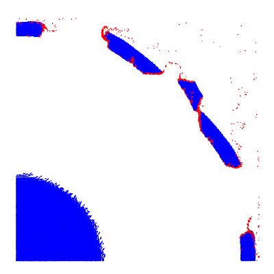
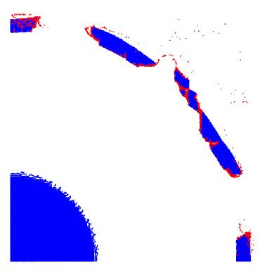
(b) 4340 Steel.                        (c) HY 100 Steel.

Figure 2: Simulations of fragmenting cylinders - two-dimensional view.

The simulation shown in Figure 2(b) was performed using material data for 4340 steel, a Mie-Grüneisen equation of state, the Johnson-Cook flow stress model, the Gurson yield condition, the Johnson-Cook damage model, and checks of both the Drucker stability postulate and the loss of hyperbolicity condition. The simulation of a HY 100 steel container shown in Figure 2(c) was performed using a Mie-Grüneisen equation of state, the MTS flow stress model, the Gurson yield condition, the Hancock-MacKenzie damage model, and the same stability checks as the 4340 steel. The material properties and the parameters used in the models are shown in Table 1. The materials are given an initial mean porosity of 0.005 using a Gaussian distribution with a standard deviation of 0.001 and a mean scalar damage value of 0.01 with a standard deviation of 0.005.

Table 1: Material Properties and Parameters for Steels.

4340 Steel properties and Johnson-Cook parameters
$\rho$	$C_{p}$	$T_{m}$	$K$	$\mu$	$\chi$
(kg/m3)	(MPa m3/kg K)	(K)	(GPa)	(GPa)
7830.0	477.0	1793.0	173.3	80.0	0.9
$A$	$B$	$C$	$n$	$m$	$D_{1}$	$D_{2}$	$D_{3}$	$D_{4}$	$D_{5}$
(MPa)	(MPa)
792.0	510.0	0.014	0.26	1.03	0.05	3.44	-2.12	0.002	0.61
HY100 Steel properties and MTS parameters
$\rho$	$C_{p}$	$T_{m}$	$K$	$\mu$	$\chi$
(kg/m3)	(MPa m3/kg K)	(K)	(GPa)	(GPa)
7860.0	477.0	2000.0	150.0	69.0	0.9
$\sigma_{a}$	$\mu_{0}$	$D$	$T_{0}$	$k/b^{3}$	$g_{0i}$	$g_{0e}$	$\dot{\epsilon}_{0i}$	$\dot{\epsilon}_{0e}$
(MPa)	(GPa)	(GPa)	(K)	(x$10^{6}$)			(x$10^{13}$)	(x$10^{7}$)
40.0	71.46	2.9	204	0.905	1.161	1.6	1.0	1.0
$p_{i}$	$q_{i}$	$p_{e}$	$q_{e}$	$\hat{\sigma}_{i}$	$a_{0}$	$a_{1}$	$a_{2}$	$a_{3}$
				(MPa)	(x$10^{9}$)			(x$10^{6}$)
0.5	1.5	0.67	1.0	1341	6	0	0	2.0758
$\theta_{IV}$	$\alpha$	$\dot{\epsilon}_{es0}$	$g_{0es}$	$\hat{\sigma}_{es0}$
(x$10^{6}$)		(x$10^{7}$)		(MPa)
200.0	3	1.0	0.112	822.0
Mie-Gruneisen equation of state parameters
$C_{0}$	$\Gamma_{0}$	$S_{\alpha}$
(m/s)
3574	1.69	1.92
GTN yield condition and porosity evolution parameters
$q_{1}$	$q_{2}$	$q_{3}$	$k$	$f_{c}$	$f_{n}$	$s_{n}$	$\epsilon_{n}$
1.5	1.0	2.25	4.0	0.05	0.1	0.3	0.1

The expected number of fragments ($N$) along the circumference of the exploding cylinder can be approximated using the following analytical result [Grady and Hightower (1992)]

$$N=2~{}\pi~{}\left(\frac{\rho~{}R_{0}~{}V^{2}}{24~{}\Gamma}\right)^{1/3}$$ (25)

where $\rho$ is the density, $R_{0}$ is the initial cylinder radius, $V$ is the expansion velocity at the radius of fracture, and $\Gamma$ is the fragmentation energy.

The fragmentation energy in tension ($\Gamma_{T}$) and in shear ($\Gamma_{S}$) are given by

$$\Gamma_{T}=\frac{K_{c}^{2}}{2~{}E}~{};~{}~{}~{}\Gamma_{S}=\frac{\rho~{}C_{p}}{\alpha}\left(\frac{9~{}\rho^{3}~{}C_{p}^{2}~{}\chi^{3}}{Y^{3}~{}\alpha^{2}\dot{\gamma}}\right)^{1/4}$$ (26)

where $K_{c}$ is the fracture toughness, $E$ is the Young’s modulus, $\rho$ is the density, $C_{p}$ is the specific heat at constant pressure, $\alpha$ is the thermal softening coefficient, $\chi$ is the thermal diffusion coefficient, $Y$ is the yield strength in simple tension, and $\dot{\gamma}$ is the shear strain rate.

For the expanding 4340 steel cylinder of that we have simulated, the relevant quantities are $\rho$ = 7830 kg/m³, $E$ = 208 GPa, $K_{c}$ = 80 MN/m^2/3, $Y$ = 792 MPa, $C_{p}$ = 477 J/kg K, $\chi$ = 1.5$\times 10^{-5}$ m²/s, $\alpha$ = 7.5$\times 10^{-4}$ /K, $R_{0}$ = 0.054 m, $V$ = 300 m/s, $\dot{\gamma}$ = 1000 /s, $\Gamma_{T}$ = 1.5 $\times 10^{4}$ J/m², and $\Gamma_{S}$ = 5.2 $\times 10^{4}$ J/m². Accordingly, the expected number of fragments (for the whole cylinder) are $N~{}(\text{tension})$ = 29 and $N~{}(\text{shear})$ = 20. For a quarter of the cylinder, the number of fragments is expected to be between 8 and 5. We get approximately 6 to 7 fragments in our simulations, which implies that our results are qualitatively acceptable. Both the steels show similar fragmentation though the exact shape of the fragments differs slightly. For this reason, the three-dimensional simulations were performed using 4340 steel and the associated models discussed above.

Figure 3 shows the fragmentation obtained from three-dimensional simulations of a cylinder with end-caps. A quarter of the geometry is modeled, assuming symmetry. The cylinder is made of 4340 steel and contains PBX 9501. The simulation is started with both materials at a temperature of 600 K. A hypoelastic constitutive model is used to determine the volumetric response of the material. The Johnson-Cook plasticity model is used to calculate the flow stress. The von Mises yield condition is used to determine the boundary of the elastic and plastic domains. A Johnson-Cook damage model is used to compute a scalar damage parameter. A uniform initial porosity is assigned to all steel particles and evolved according to the models discussed in the previous section. A particle is deemed to have failed when the modified TEPLA-F condition is satisfied, the temperature is more than the melting temperature, or the Drucker stability postulate/loss of hyperbolicity condition is satisfied. Upon failure, the particle stress is set to zero.

(a) Fragments of the container.                        (b) Gases escaping from the container.

Figure 3: Simulations of fragmenting cylinders - three-dimensional view.

The simulations capture some of the qualitative features observed in the experiments of steel cylinders heated using heat tapes. Some high particle velocities are observed upon failure. Simulations have shown that these velocities are due to some increase in the total energy due to the setting of the particle stress to zero. Computations where failed particles are converted into a material with a different velocity field are currently under way along with other validation efforts to quantify the error in the calculations.

Simulations have also been performed on containers heated by a pool fire. Four snapshots of one such simulation for 4340 steel using the Johnson-Cook plasticity and damage models, a Mie-Gruneisen equation of state, the von Mises yield condition and uniform initial porosity are shown in Figure 4.

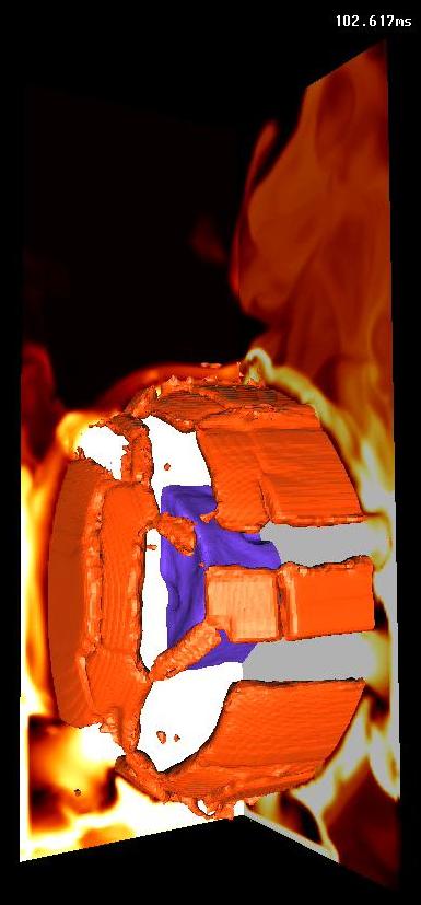
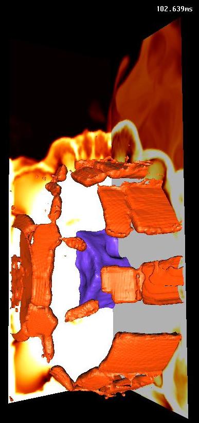
Figure 4: Simulations of fragmentation of a cylinder heated by a fire.

The fire is simulated by a hot jet of air and interacts with the container via heat conduction and momentum transport. After some time, the contents of the container reach ignition temperature and reaction proceeds rapidly. Axial cracks open up in the container that are qualitatively similar to those observed in experiments. These cracks join to form fragments which interact with the fire. More details of such simulations can be found elsewhere [Guilkey et al. (2004)]. Validation of the pool fire and container interaction scenario is currently being performed in collaboration with researchers at the Lawrence Livermore National Laboratory.

6 Summary and Conclusions

A computational scheme for the simulation of the fragmentation of cylinders due to interaction with gases from a reacting high energy material has been presented. The scheme allows for the incorporation of various plasticity models, yield conditions, damage models, equations of state, and stability checks within the same stress update code. A number of such models have been listed and the corresponding material properties and parameters for two steels have been collected from various sources and presented in a compact form.

Simulations of exploding cylinders in two-dimensions have been compared with analytical solutions for the expected number of fragments and found to provide qualitative agreement. Three-dimensional simulations also show qualitative agreement with experiments in the directions of the dominant cracks. Snapshots from the simulation of a fully coupled container-fire simulation have also shown qualitative agreement with experiments.

Two issues that have been identified as important for the simulation are the conservation of energy and mesh dependence of the results. Validation simulations that are currently underway have shown that energy is better conserved when particles are converted into a material with a different velocity field after failure (rather than setting the stress to zero upon failure). Results of these tests will be presented in future work. In the absence of a limiting length scale in the computation, strongly mesh dependent behavior can be expected in the softening regime of the stress-strain relationship. This mesh dependence occurs when we use temperature dependent elastic/plastic constitutive equations and when we degrade the yield strength of the porous material using porosity. One way of minimizing mesh dependence is to use a rate-dependent stress update algorithm. However, such an approach is not sufficient to remove the effects of all the possible causes of mesh dependence. Validation experiments are currently underway to determine the extent of mesh dependence and nonlocal/gradient plasticity approaches that can be formulated for the material point method. Overall, the material point method appears to be a promising approach for simulating high rate, coupled fluid-structure interaction problems and fragmentation.

7 Acknowledgments

This work was sponsored by the Department of Energy Accelerated Supercomputing Initiative (DOE-ASCI), Lawrence Livermore National Laboratory and the Center for the Simulation of Accidental Fires and Explosions (C-SAFE), University of Utah. The author would like to acknowledge Dr. Steve Parker and his team in the School of Computing, University of Utah, for providing the infrastructure for parallel computing and visualization. Thanks also go to Drs. James Guilkey and Todd Harman from the Department of Mechanical Engineering, University of Utah, for providing the fluid-structure interaction code and performing the large container and fluid-structure interaction simulations on supercomputers at the Los Alamos National Laboratory.

References

- Armstrong et al. (1999) Armstrong, R., Gammon, D., Geist, A., Keahey, K., Kohn, S., McInnes, L., Parker, S., and Smolinski, B. (1999). “Toward a Common Component Architecture for high-performance scientific computing.” Proc. 1999 Conference on High Performance Distributed Computing.
- Bardenhagen et al. (2001) Bardenhagen, S. G., Guilkey, J. E., Roessig, K. M., BrackBill, J. U., Witzel, W. M., and Foster, J. C. (2001). “An improved contact algorithm for the material point method and application to stress propagation in granular material.” Computer Methods in the Engineering Sciences, 2(4), 509–522.
- Bardenhagen and Kober (2004) Bardenhagen, S. G. and Kober, E. M. (2004). “The generalized interpolation material point method.” Comp. Model. Eng. Sci. to appear.
- Bazant and Belytschko (1985) Bazant, Z. P. and Belytschko, T. (1985). “Wave propagation in a strain-softening bar: Exact solution.” ASCE J. Engg. Mech, 111(3), 381–389.
- Becker (2002) Becker, R. (2002). “Ring fragmentation predictions using the gurson model with material stability conditions as failure criteria.” Int. J. Solids Struct., 39, 3555–3580.
- Bennett et al. (1998) Bennett, J. G., Haberman, K. S., Johnson, J. N., Asay, B. W., and Henson, B. F. (1998). “A constitutive model for non-shock ignition and mechanical response of high explosives.” J. Mech. Phys. Solids, 46(12), 2303–2322.
- Borvik et al. (2001) Borvik, T., Hopperstad, O. S., Berstad, T., and Langseth, M. (2001). “A computational model of viscoplastcity and ductile damage for impact and penetration.” Eur. J. Mech. A/Solids, 20, 685–712.
- Chu and Needleman (1980) Chu, C. C. and Needleman, A. (1980). “Void nucleation effects in biaxially stretched sheets.” ASME J. Engg. Mater. Tech., 102, 249–256.
- Coplien (1992) Coplien, J. O. (1992). Advanced C++ Programming Styles and Idioms. Addison-Wesley, Reading, MA.
- de St. Germain et al. (2000) de St. Germain, J. D., McCorquodale, J., Parker, S. G., and Johnson, C. R. (2000). “Uintah: a massively parallel problem solving environment.” Ninth IEEE International Symposium on High Performance and Distributed Computing. IEEE, Piscataway, NJ, 33–41.
- Drucker (1959) Drucker, D. C. (1959). “A definition of stable inelastic material.” J. Appl. Mech., 26, 101–106.
- Follansbee and Kocks (1988) Follansbee, P. S. and Kocks, U. F. (1988). “A constitutive description of the deformation of copper based on the use of the mechanical threshold stress as an internal state variable.” Acta Metall., 36, 82–93.
- Goto et al. (2000) Goto, D. M., Bingert, J. F., Chen, S. R., Gray, G. T., and Garrett, R. K. (2000). “The mechanical threshold stress constitutive-strength model description of HY-100 steel.” Metallurgical and Materials Transactions A, 31A, 1985–1996.
- Goto et al. (2000) Goto, D. M., Bingert, J. F., Reed, W. R., and Garrett, R. K. (2000). “Anisotropy-corrected MTS constitutive strength modeling in HY-100 steel.” Scripta Mater., 42, 1125–1131.
- Grady and Hightower (1992) Grady, D. E. and Hightower, M. M. (1992). “Natural fragmentation of exploding cylinders.” Shock-Wave and High-Strain-Rate Phenomena in Materials, M. A. Meyers, L. E. Murr, and K. P. Staudhammer, eds., Marcel Dekker Inc., New York, chapter 65, 713–721.
- Guilkey et al. (2004) Guilkey, J. E., Harman, T. B., Kashiwa, B. A., and McMurtry, P. A. (2004). “An Eulerian-Lagrangian approach to large deformation fluid-structure interaction problems. Submitted.
- Gurson (1977) Gurson, A. L. (1977). “Continuum theory of ductile rupture by void nucleation and growth: Part 1. Yield criteria and flow rules for porous ductile media.” ASME J. Engg. Mater. Tech., 99, 2–15.
- Hancock and MacKenzie (1976) Hancock, J. W. and MacKenzie, A. C. (1976). “On the mechanisms of ductile failure in high-strength steels subjected to multi-axial stress-states.” J. Mech. Phys. Solids, 24, 147–167.
- Hao et al. (2000) Hao, S., Liu, W. K., and Qian, D. (2000). “Localization-induced band and cohesive model.” J. Appl. Mech., 67, 803–812.
- Hill and Hutchinson (1975) Hill, R. and Hutchinson, J. W. (1975). “Bifurcation phenomena in the plane tension test.” J. Mech. Phys. Solids, 23, 239–264.
- Johnson and Cook (1983) Johnson, G. R. and Cook, W. H. (1983). “A constitutive model and data for metals subjected to large strains, high strain rates and high temperatures.” Proc. 7th International Symposium on Ballistics. 541–547.
- Johnson and Cook (1985) Johnson, G. R. and Cook, W. H. (1985). “Fracture characteristics of three metals subjected to various strains, strain rates, temperatures and pressures.” Int. J. Eng. Fract. Mech., 21, 31–48.
- Johnson and Addessio (1988) Johnson, J. N. and Addessio, F. L. (1988). “Tensile plasticity and ductile fracture.” J. Appl. Phys., 64(12), 6699–6712.
- Long and Wight (2002) Long, G. T. and Wight, C. A. (2002). “Thermal decomposition of a melt-castable high explosive: isoconversional analysis of TNAZ.” J. Phys. Chem. B, 106, 2791–2795.
- Perzyna (1998) Perzyna, P. (1998). “Constitutive modelling of dissipative solids for localization and fracture.” Localization and Fracture Phenomena in Inelastic Solids: CISM Courses and Lectures No. 386, P. P., ed., SpringerWien, New York, 99–241.
- Ramaswamy and Aravas (1998a) Ramaswamy, S. and Aravas, N. (1998a). “Finite element implementation of gradient plasticity models Part I: Gradient-dependent yield functions.” Comput. Methods Appl. Mech. Engrg., 163, 11–32.
- Ramaswamy and Aravas (1998b) Ramaswamy, S. and Aravas, N. (1998b). “Finite element implementation of gradient plasticity models Part II: Gradient-dependent evolution equations.” Comput. Methods Appl. Mech. Engrg., 163, 33–53.
- Rudnicki and Rice (1975) Rudnicki, J. W. and Rice, J. R. (1975). “Conditions for the localization of deformation in pressure-sensitive dilatant materials.” J. Mech. Phys. Solids, 23, 371–394.
- Steinberg et al. (1980) Steinberg, D. J., Cochran, S. G., and Guinan, M. W. (1980). “A constitutive model for metals applicable at high-strain rate.” J. Appl. Phys., 51(3), 1498–1504.
- Sulsky et al. (1994) Sulsky, D., Chen, Z., and Schreyer, H. L. (1994). “A particle method for history dependent materials.” Comput. Methods Appl. Mech. Engrg., 118, 179–196.
- Sulsky et al. (1995) Sulsky, D., Zhou, S., and Schreyer, H. L. (1995). “Application of a particle-in-cell method to solid mechanics.” Computer Physics Communications, 87, 236–252.
- Tvergaard and Needleman (1984) Tvergaard, V. and Needleman, A. (1984). “Analysis of the cup-cone fracture in a round tensile bar.” Acta Metall., 32(1), 157–169.
- Tvergaard and Needleman (1990) Tvergaard, V. and Needleman, A. (1990). “Ductile failure modes in dynamically loaded notched bars.” Damage Mechanics in Engineering Materials: AMD 109/MD 24, J. W. Ju, D. Krajcinovic, and H. L. Schreyer, eds., American Society of Mechanical Engineers, New York, NY, 117–128.
- Zocher et al. (2000) Zocher, M. A., Maudlin, P. J., Chen, S. R., and Flower-Maudlin, E. C. (2000). “An evaluation of several hardening models using Taylor cylinder impact data.” Proc. , European Congress on Computational Methods in Applied Sciences and Engineering, ECCOMAS, Barcelona, Spain.