WIS/02/12-JAN-DPPA

1 Introduction

Seiberg duality [1] is a powerful tool to study supersymmetric theories with four supercharges. When engineering a supersymmetric theory on D-branes in string theory, Seiberg duality typically arises as a change of “brane basis” of some sort.

In three dimensional theories with Chern-Simons (CS) interactions, some Seiberg dualities have been proposed by using branes suspended between branes in type IIB string theory [2, 3, 4, 5]. In all these examples, the field theory has matter in real representations of the gauge group, and the duality is suggested by the brane creation effect when 5-branes cross each other [6].

In this paper we study Seiberg duality for CS quiver theories constructed from type IIA string theory, following [8, 9, 10, 11, 12]. There are at least two advantages to the type IIA approach. Firstly, it allows to engineer quivers with chiral matter content (by “chiral” we mean matter fields in non-real representations). Secondly, the connection between quivers and M2-branes on a Calabi-Yau (CY) fourfold singularity, which is the motivation to study such quivers [13], is rather transparent: The IIA setup is the KK reduction of the M-theory setup along a wisely chosen M-theory circle, and the quiver is the one describing D-branes at a CY threefold singularity in type IIA.

Recently, precise rules for Seiberg duality in three dimensional chiral quiver gauge theories were found in [14] from a careful field theory analysis. They generalize the Giveon-Kutasov rules [3] that govern the non-chiral case. In this work we will provide a string theory explanation for such rules. The idea is very simple, once we review in some detail the beautiful relation between supersymmetric quiver theories and D-branes at Calabi-Yau threefold singularities: 3d Seiberg duality is a double brane mutation. This point of view builds on a similar understanding for 4d Seiberg duality [15, 16].

Consider a conical CY₃ $Y$ and a partial resolution $\pi:\tilde{Y}\rightarrow Y$. On any $\tilde{Y}$ we can consider probe branes (D2-branes in particular), and there exists a well-known relation between the branes on $\tilde{Y}$ and a quiver $\mathcal{Q}$, defined abstractly. Any D-brane corresponds to some “representation” of the quiver. In that context Seiberg duality for D-branes on $\tilde{Y}$ is well understood as a change of brane basis [17, 18, 19, 20]; in the case of interest to us the change of basis will be related to sheaf mutations [15, 16].

The CS quivers we consider are engineered by considering D2-branes on a CY₃ $Y$ fibered on a line $\{r_{0}\}=\mathbb{R}$. There are rather generic RR fluxes, including the $F_{2}$ flux corresponding to a non-trivial M-theory fibration, and the whole setup corresponds to M2-branes at the tip of a CY₄ cone. The CY₃ $Y$ is singular at the origin $r_{0}=0$, but it is partially resolved for any $r_{0}\neq 0$. Considering $Y$ as an algebraic variety, the partial resolution $\tilde{Y}$ might not be the same at $r_{0}>0$ or $r_{0}<0$, and we have thus two distinct CY₃ varieties $\tilde{Y}_{\pm}$. The CS quiver gauge theories for D-branes on such a setup can be found by taking an appropriate “average” of the theories we would obtain from $\tilde{Y}_{-}$ and $\tilde{Y}_{+}$ separately. The Chern-Simons levels are induced on the branes by the RR background fluxes.

In that setup the 3d Seiberg duality is a doubling of the mutation procedure, performed both on $\tilde{Y}_{-}$ and $\tilde{Y}_{+}$. We will explain this in detail after introducing the necessary formalism.

In section 2 we review the deep relationship that exists between D-branes at $Y$ and a quiver $\mathcal{Q}$. Considered abstractly, the quiver is just an oriented graph. To that abstract quiver we can associate a choice of gauge group $\prod_{i}U(N_{i})$, which is part of a choice of quiver representation: different representations correspond to different D-brane configurations on $Y$. When dealing with D3-brane quivers this point of view is a bit less useful, because the choice of ranks $N_{i}$ are essentially fixed by anomaly cancelation. Our 3d theories have completely generic ranks $N_{i}$, which makes the abstract point of view more necessary. More background material is provided in several Appendices.

In section 3 we start by reviewing some relevant facts about the moduli space of Chern-Simons quivers, following the recent work [12]. We then present the formalism of [11, 12] providing the map from (some) M-theory/IIA backgrounds to CS quivers. We next proceed to state our main result, relating 3d Seiberg duality for chiral quivers to brane mutations.

In section 4 we apply our formalism to the CS theories dual to $Y^{p,q}(\mathbb{C}\mathbb{P}^{2})$, we derive Seiberg dual quivers for the whole family of theories of [11], and we provide some consistency checks of the result. Our mutation perpective on 3d Seiberg duality has also been applied to the study of many toric examples in [12].

Finally, in section 5, which is independent from the rest of the paper, we briefly comment on the correct brane charge to use in the formalism of [11, 12], allowing to generalize those works to cases when the IIA background contains $F_{0}$ flux and has no eleven dimensional M-theory dual [21].

2 D-branes and Seiberg duality

In this section we review supersymmetric quiver theories from the perspective of D-branes and the precise sense in which Seiberg duality for quivers arises as a change of “brane basis”.

2.1 $CY_{3}$ Quivers and Seiberg duality

A quiver $\mathcal{Q}$ is an oriented graphs which can have multiples arrows between the nodes. It also allows for closed loops. Let $Q_{0}=\{1,2,\cdots,G\}$ be the set of nodes (indexed by the letters $i,j$) and $Q_{1}=\{a_{1},a_{2},\cdots,a_{E}\}$ the set of arrows; the notation $a_{ij}$ denotes an arrow from $i$ to $j$. We are interested in quivers with superpotential $(\mathcal{Q},W)$. The superpotential is a formal sum of words (up to cyclic permutation),

$$W=\sum_{L}a_{i_{1}i_{2}}a_{i_{2}i_{3}}\cdots a_{i_{|L|}i_{1}}\,,$$ (2.1)

where the summands correspond to closed loops $L=\{i_{1}i_{2}\cdots i_{|L|}\}$ in the quiver. We denote by $Q_{2}$ the set of all loops appearing in $W$. The quiver with superpotential is a quiver with relations $\{F_{a}=0\}$, where the relations between the path are given by formal derivation

$$F_{a}=\frac{\partial}{\partial a}W\,,\qquad\qquad\forall\,a\in Q_{1}\,.$$ (2.2)

In fact the quivers we consider are even more restricted and correspond to $CY_{3}$ quivers. We define (rather tautologically) a $CY_{3}$ quiver as a quiver that arises from D-branes at a CY₃ cone; see [22] and references therein for a mathematical definition of the concept.

Our motivation to study $\mathcal{Q}$ is that it summarizes the classical Lagrangian of a supersymmetric field theory, which is itself the low energy theory on D-branes on a Calabi-Yau threefold. The more abstract point of view that is taken here is however very useful even for physicists — see e.g. [23, 24].

The basic notion that we will need is that of a quiver representation. Some general facts on quivers are reviewed in Appendix A. A representation $X$ of $\mathcal{Q}$ is a choice of vector space $V_{i}$ for each node and a choice of linear map $X_{a}:V_{i}\rightarrow V_{j}$ for each arrow $a=a_{ij}$, such that the $X_{a}$’s satisfy the relations (2.2). More concretely, we consider only complex vector spaces $V_{i}=\mathbb{C}^{N_{i}}$ and thus the linear maps $X_{a}$ are complex-valued $N_{j}\times N_{i}$ matrices.

A morphism $\phi$ between two quiver representations $X$ and $X^{\prime}$ is a set of $G$ linear maps $\phi_{i}:V_{i}\rightarrow V_{i}^{\prime}$ such that

$$\phi_{i}X_{a}^{\prime}=X_{a}\phi_{j}\,,\qquad\forall\,a=a_{ij}\in Q_{1}\,.$$ (2.3)

If $\phi$ is injective, we say that $X$ is a subrepresentation of $X^{\prime}$. On the other end two representations $X$, $X^{\prime}$ are called isomorphic (or gauge equivalent) if there exist a bijective morphism $\phi:X\rightarrow X^{\prime}$. We should really only consider equivalence classes under such relations. The dimension vector of any representation $X$ is defined as

$$\text{dim}\,X\equiv(\text{dim}\,V_{1},\cdots,\text{dim}\,V_{G})=(N_{1},\cdots,N_{G})\equiv\bm{N}.$$ (2.4)

A choice of dimension vector determines a $\mathcal{N}=1$ supersymmetric quiver theory $(\mathcal{Q},\bm{N})$ in four dimensions, and more generally a theory with four supercharges in dimension $\leq 4$. The gauge group is

$$\mathcal{G}=U(N_{i})\times\cdots\times U(N_{G})$$ (2.5)

and the arrows $a_{ij}\in Q_{1}$ correspond to chiral superfields $X_{ij}$ in bifundamental representations. In the following we will assume there are no arrow $a:i\rightarrow i$ (no chiral multiplets in adjoint representations), although this case can be discussed as well [24]. So far everything in the discussion is holomorphic, and it is well known that as far as the F-terms are concerned the actual gauge group of the theory $(\mathcal{Q},\bm{N})$ is complexified, $\mathcal{G}_{\mathbb{C}}=\prod_{i=1}^{G}\,GL(N_{i},\mathbb{C})$. The set of all quiver representations (more precisely $\mathcal{G}_{\mathbb{C}}$ equivalence classes of representations) with fixed dimension vector correspond to all possible VEVs for the fields $X_{ij}$ which satisfy the F-term relations (2.2), quotiented by $\mathcal{G}_{\mathbb{C}}$. In other words, the moduli space of quiver representations of fixed dimension vector $\bm{N}$ is the same as the vacuum moduli space of physicists. For the moment we leave aside the issue of how exactly one solves the D-term equations of the quiver theory, content with the fact that such a solution always exists along the complexified gauge orbits [25] (in the absence of FI parameters).

To discuss Seiberg duality for quivers in full generality, we would need to introduce a few more abstract facts about quivers. In the following we will discuss some simpler notions of Seiberg duality, which are less general, but for completeness we provide a summary of the general case in Appendix A.

2.2 Purely chiral quivers and quiver mutations

The approach to Seiberg duality of [24], reviewed in Appendix, is very beautiful and general, but explicit computations are a bit hard for anyone not familiar with higher mathematics. In the following we present a more concrete definition of Seiberg duality based on the mathematical work of [26]. It only applies to a subset of CY₃ quivers, but it will turn out to be the most interesting ones for our later purposes.

Let us denote by $A$ the antisymmetric adjacency matrix of the quiver $\mathcal{Q}$, defined by

$$A_{ij}=n_{ij}-n_{ji}\,,$$ (2.6)

where $n_{ij}$ is the number of arrows $a_{ij}$ from $i$ to $j$. We call a quiver “purely chiral” if $A$ is enough to reconstruct $\mathcal{Q}=(Q_{0},Q_{1})$, namely if there are no loops of two arrows ($ab$ such that $a:i\rightarrow j$ and $b:j\rightarrow i$) and no arrow $a:i\rightarrow i$ from a node to itself.

A quiver mutation $\mu_{k}(\mathcal{Q})$ on a node $k\in Q_{0}$ is defined as expected from physics: We reverse all the arrows of the form $a_{ik}$ and $a_{kj}$, introduce new arrows $m_{ij}=a_{ik}a_{kj}$ and a new superpotential $\mu_{k}(W)=W+\tilde{a}_{ki}\,m_{ij}\,\tilde{a}_{jk}$ written in term of the new arrows, and finally remove any arrows that appear in a term of order $2$ in the new $W$ while imposing the corresponding relations $F_{a}=0$. Of course this is nothing but the usual prescription for Seiberg duality [1], including the integrating out of massive mesons. The interest for us is that is has been abstracted to a quiver $\mathcal{Q}$ instead of any particular quiver representation $(\mathcal{Q},\bm{N})$. The effect on the adjacency matrix is a so-called matrix mutation at position $k$ [26]

$$\mu_{k}\left(A_{ij}\right)\,=\,\begin{cases}-A_{ij}\qquad&\quad\text{if}\;i=k\;\text{or}\;j=k\\ A_{ij}+\frac{1}{2}\left(|A_{ik}|A_{kj}+A_{ik}|A_{kj}|\right)&\quad\text{otherwise}\end{cases}$$ (2.7)

For a given supersymmetric theory $(\mathcal{Q},\bm{N})$, the mutation $\mu_{k}$ can give rise to different actions on the dimension vector $\bm{N}$ depending on the precise vacuum of $(\mathcal{Q},\bm{N})$ [27]. Two cases are of particular physical interest:

$$\mu_{k}^{L}\,: \,\quad N_{i}^{\prime}=N_{i}\,,\qquad\text{if}\;i\neq k\,,\qquad\quad N_{k}^{\prime}=-N_{k}+\sum_{i}\,[A_{ik}]_{+}N_{i}\,,$$ (2.8)

$$\mu_{k}^{R}\,: \,\quad N_{i}^{\prime}=N_{i}\,,\qquad\text{if}\;i\neq k\,,\qquad\quad N_{k}^{\prime}=-N_{k}+\sum_{j}\,[A_{kj}]_{+}N_{j}\,$$

(with the definition $[x]_{+}=\max(x,0)$), which we call left- and right-mutation of quiver representation, respectively. This reproduces the Seiberg duality of four dimensional quivers (at the classical level), but it is also more general. In four dimensions, anomaly cancelation restricts the allowed theories $(\mathcal{Q},\bm{N})$ according to the condition

$$A\bm{N}=0\,.$$ (2.9)

In three dimensions there is no such restriction.

2.3 From D-branes to quivers

Consider a background space-time $\mathbb{R}^{1,3}\times Y$ in type II string theory, where $Y$ is a non-compact conical Calabi-Yau threefold, together with some D-branes transverse to $Y$ —for our purposes these will be D3-branes in type IIB or D2-branes in type IIA. At the conical singularity of $Y$, these D-branes usually decay marginally into a bound state of so-called fractional branes, which we denote $\{E^{\vee}_{i}\}_{i=1,\cdots,G}$. The fractional branes can be loosely thought of as D-branes wrapped on vanishing cycles [28]. The local dynamics of the fractional branes in well encoded in a supersymmetric quiver gauge theory, which describes the massless open string sector of the theory.

In general we cannot compute the open string spectrum at the CY singularity $Y$ directly since we lack a perturbative definition of string theory on such spaces. Nevertheless the question of finding the quiver $\mathcal{Q}_{Y}$ corresponding to any given $Y$ has been much studied in the past decade [19, 30, 31, 32], and it has been solved in the toric case [33, 34, 35, 36].

Consider a crepant resolution $\tilde{Y}$ of the cone $Y$,

$$\pi:\tilde{Y}\rightarrow Y\,,\qquad\qquad\text{with}\qquad\mathcal{O}_{\tilde{Y}}(K)\cong\pi^{*}\mathcal{O}_{Y}(K)\,,$$ (2.10)

where $\mathcal{O}_{M}(K)$ denotes the canonical line bundle (or canonical sheaf) of a variety $M$. For simplicity we will restrict our study to the case when $\tilde{Y}$ has one and only one exceptional divisor $B_{4}$. The surface $B_{4}$ is then a 2-complex dimensional Fano variety (not necessarily smooth), and we have

$$\tilde{Y}\,=\,\mathcal{O}_{B_{4}}(K)\,.$$ (2.11)

The main reason to write $\tilde{Y}$ as (2.11) is that fractional branes must be wrapped on compact cycles, and therefore correspond to branes on $B_{4}$. As reviewed in Appendix B, our branes are generally chain complexes of sheaves (B-branes),

$$\mathsf{E}\;=\;\cdots\rightarrow E_{(-2)}\rightarrow E_{(-1)}\rightarrow E_{(0)}\rightarrow E_{(1)}\rightarrow\cdots\;.$$ (2.12)

In this work we will only be concerned with the charges of the branes, so that we can skip most of the B-brane category mumbo-jumbo. The charge of a B-brane (2.12) is defined as its Chern character

$$ch(\mathsf{E})=\sum_{n}(-1)^{n}\,ch(E_{(n)})\;,$$ (2.13)

where $ch(E_{(n)})$ are the Chern characters of the individual sheaves. We refer to section 5 for a more careful discussion of brane charges. To discuss the most general brane charges we consider a full resolution $\pi:\tilde{B}_{4}\rightarrow B_{4}$, which is what the B-model probes. Let us denote

$$\mathcal{C}_{\alpha}\in H^{2}(\tilde{B}_{4},\mathbb{Z})\,,\qquad\alpha=1,\cdots,m\,,\qquad\quad\quad\mathcal{C}_{\alpha}\mathcal{C}_{\beta}=\mathcal{I}_{\alpha\beta}\,.$$ (2.14)

a primitive basis of 2-cycles, with $\mathcal{I}$ the intersection matrix. There are $G\equiv m+2$ charges for the compactly supported branes (branes wrapping $B_{4}$, $\mathcal{C}_{\alpha}$ or a point), and we denote the Chern character (2.13) of a generic brane $\mathsf{E}$ by the covector

$$\bm{Q}_{\text{branes}}(\mathsf{E})\,=\,ch(\mathsf{E})\,=\,(rk(\mathsf{E}),c_{1}(\mathsf{E}),ch_{2}(\mathsf{E}))\,.$$ (2.15)

The Euler character of a pair of branes is defined by

$$\chi(\mathsf{E}_{i},\mathsf{E}_{j})\,\equiv\,\sum_{q}(-1)^{q}\,\mathrm{dim}\,\mathrm{Ext}^{q}(\mathsf{E}_{i},\mathsf{E}_{j})\;,$$ (2.16)

and can be computed by the Riemann-Roch theorem:

$$\chi(\mathsf{E}_{i},\mathsf{E}_{j})\,=\,\int_{\tilde{B}_{4}}\,ch(\mathsf{E}_{i}^{*})\,ch(\mathsf{E}_{j})\,Td(\tilde{B}_{4})\;.$$ (2.17)

We can conveniently rewrite this in matrix notation,

$$\chi(\mathsf{E}_{i},\mathsf{E}_{j})=ch(\mathsf{E}_{i})\,\mathbf{X}_{\tilde{B}_{4}}\,ch(\mathsf{E}_{j})^{T}\;,\qquad\quad\text{with}\qquad\mathbf{X}_{\tilde{B}_{4}}=\begin{pmatrix}1&\frac{1}{2}c_{1}&1\\ -\frac{1}{2}c_{1}&-\mathcal{I}&0\\ 1&0&0\end{pmatrix}\,,$$ (2.18)

where $\mathcal{I}$ is defined in (2.14) and $c_{1}=c_{1}(\tilde{B}_{4})$; thus the matrix $\mathbf{X}_{\tilde{B}_{4}}$ is intrinsic to the geometry we consider.

Suppose that we are given a collection of $G$ sheaves

$$\mathcal{E}=\{E_{1},E_{2},\cdots,E_{G}\}$$ (2.19)

which generates all the B-branes on $\tilde{B}_{4}$. Such a collection is called a tilting collection if moreover

$$\text{Ext}^{q}(E_{i},E_{j})=0\,\qquad\qquad\forall q>0\,.$$ (2.20)

We refer to [37] for a good introduction to Ext groups. Given the tilting collection (2.19), we expect that the sheaves

$$\mathsf{P}_{i}\equiv\pi^{\ast}E_{i}$$ (2.21)

form a tilting collection on the resolved cone $\pi:\tilde{Y}\rightarrow Y$; see for instance [38] for similar relations. We will leave this as a conjecture. For $\{\mathsf{P}_{i}\}$ a tilting collection is follows very generally that the algebra

$$\mathcal{A}=\mathrm{End}(\,\oplus_{i=1}^{G}\,\mathsf{P}_{i})^{\,\text{op}}$$ (2.22)

is the path algebra of a fractional brane quiver. We are more interested in the collection of fractional brane, denoted

$$\mathcal{E}^{\vee}=\{\mathsf{E}^{\vee}_{1},\mathsf{E}^{\vee}_{2},\cdots,\mathsf{E}^{\vee}_{G}\}\,.$$ (2.23)

In some simple cases they can be written explicitly through sheave mutations [31, 15, 16, 32]. To compute their charge we only need to know that they are dual to the $E_{i}$’s in the sense of the Euler character,

$$\chi(E_{i},\mathsf{E}_{j}^{\vee})=\delta_{ij}\,,$$ (2.24)

and we take (2.24) as our practical definition of (2.23). Let us also define the matrix

$$S_{ij}\equiv\chi(E_{i},E_{j})=\mathrm{dim}\,\text{Hom}(E_{i},E_{j})\;,$$ (2.25)

where the second equality holds because of (2.20). We introduce the two $G\times G$ matrices

$$Q=\begin{pmatrix}ch(E_{1})\\ \vdots\\ ch(E_{G})\end{pmatrix}\;,\qquad\qquad Q^{\vee}=\begin{pmatrix}ch(\mathsf{E}_{1}^{\vee})\\ \vdots\\ ch(\mathsf{E}_{G}^{\vee})\end{pmatrix}\;.$$ (2.26)

In term of these charge matrices we can rewrite (2.24) and (2.25) in a compact way:

$$Q^{\vee T}=(\mathbf{X}_{\tilde{B}_{4}})^{-1}\,Q^{-1}\,,\qquad\qquad S=Q\,\mathbf{X}_{\tilde{B}_{4}}\,Q^{T}\,.$$ (2.27)

The antisymmetric adjacency matrix $A$ of the quiver $\mathcal{Q}$ associated to (2.22) can be found from $S$, according to

$$A\equiv S^{-1T}-S^{-1}\,.$$ (2.28)

Assuming the correct quiver is purely chiral, this completely determines it as a graph. This simple technique does not determine the quiver superpotential, however, which can in principle be extracted by more careful computations in the B-brane category [39].

The matrix $Q^{\vee}$ is the dictionnary that allows to translate between the brane charge basis (2.15) and the fractional brane basis (ranks of the gauge groups in the quiver), according to

$$\bm{Q}_{\text{branes}}=\bm{N}\,Q^{\vee}\,.$$ (2.29)

In particular, for a point-like D-brane $\mathcal{O}_{p}$, we have $\bm{Q}_{\text{branes}}=(0,\cdots,0,1)$, and

$$\bm{N}\,=\,(0,\cdots,0,1)(Q^{\vee})^{-1}\,=(rk(E_{1}),\cdots,rk(E_{G}))\equiv(r_{1},\cdots,r_{G})=\bm{r}\,,$$ (2.30)

namely the ranks of the supersymmetric quiver are given by the ranks of the sheaves in the tilting collection (2.19), which we will denote $(r_{i})$. Remark that the theory on $\mathcal{O}_{p}$ will have an Abelian gauge group if and only if the corresponding tilting collection is a collection of line bundles —for instance this is what happens in so-called toric quivers [40, 41].

2.4 Mutations, branes and quivers

Given a particular tilting collection on $B_{4}$ called a (complete) strongly exceptional collection, it is known that one can generate another strongly exceptional collection through so-called sheaf mutations [16].

We conjecture that, given a tilting collection (2.19), it is possible to obtain another collection of B-branes which is again tilting by a similar mutation of sheaves, which exactly parallels the notion of quiver mutation. Let $\mathcal{Q}$ be the quiver associated to the tilting collection $\mathcal{E}$ and let us choose an element $E_{k}\in\mathcal{E}$. Let us denote by $I_{L}\subset Q_{0}$ (resp. $I_{R}\subset Q_{0}$) the set of nodes which are connected to $k$ by incoming (resp. outgoing) arrows in $\mathcal{Q}$. At the level of branes charges, a “left (resp. right) mutation” on $E_{k}$ is defined by

$$\mu_{k}^{L}\,: \,\quad ch(E_{i}^{\prime})=ch(E_{i})\,,\quad\text{if}\;i\neq k\,,\qquad\quad ch(E_{k}^{\prime})=-ch(E_{k})+\sum_{i\in I_{L}}\,A_{ik}\,ch(E_{i})\,,$$ (2.31)

$$\mu_{k}^{R}\,: \,\quad ch(E_{i}^{\prime})=ch(E_{i})\,,\quad\text{if}\;i\neq k\,,\qquad\quad ch(E_{k}^{\prime})=-ch(E_{k})+\sum_{j\in I_{R}}\,A_{kj}\,ch(E_{j})\,,$$

where $A$ is defined in (2.28). One can consider (2.31) as our working definition of brane mutation, at the level of charges (which is all we need in this work).

We introduce a matrix $M_{k}$ (also written $M_{(k;L)}$ or $M_{(k;R)}$ if we need to distinguish between left or right mutation) such that (2.31) can be written

$$\mu_{k}^{L,R}\,:\;Q\;\mapsto\;Q^{\prime}\,=\,M_{(k;L,R)}\,Q\,,$$ (2.32)

in term of the charge matrix $Q$ in (2.26). Remark that $M_{k}^{2}=1$, and thus applying the mutation twice at the same node gives back the original collection; however if $M_{k}$ is a left mutation of the collection $\mathcal{E}$ it will be a right mutation of the collection $\mathcal{E}^{\prime}=\mu_{k}(\mathcal{E})$, and vice versa. We can easily see that

$$S^{\prime}\,=\,M_{k}\,S\,M_{k}^{T}\,,\,\qquad\qquad A^{\prime}=M_{k}^{T}\,A\,M_{k}\,,$$ (2.33)

and

$$Q^{\vee}\phantom{}{}^{\prime}=M^{T}_{k}\,Q^{\vee}\,.$$ (2.34)

Comparing to (2.7) one can see that brane mutation and quiver mutation of a purely chiral quiver are one and the same thing.

From (2.34) and (2.29) it also follows that the dimension vector of a quiver representation transforms as

$$\bm{N}^{\prime}=M_{k}\bm{N}\,,$$ (2.35)

in agreement with the definitions (2.8).

2.5 Kähler moduli space and quiver locus

In the previous subsections we introduced some B-branes states $\mathcal{E}=\{\mathsf{E}_{i}^{\vee}\}$ on a resolved cone $\tilde{Y}$ and we reviewed how such a set of branes is related to a supersymmetric quiver theory. To relate this to the intuitive notion of fractional branes at a singularity, we should show that these $\mathsf{E}^{\vee}$’s are indeed individually BPS and mutually BPS, when placed at the tip of $Y$. While in some rare cases [42, 15] this can be proven directly using mirror symmetry, in general we will simply assume that this is true and see what it entails.

The Kähler moduli space $\mathcal{M}_{K}$ of $Y$ has real dimension $2m$. Let $Z(\mathsf{E})$ be the central charge of a B-brane $\mathsf{E}$ (see Appendix C for more details). A B-brane is BPS at a given point in $\mathcal{M}_{K}$ if it is $\Pi$-stable [43]; we do not review this notion here, but we will review the quiver analog of $\Pi$-stability in the following. The point-like D-brane $\mathcal{O}_{p}$ is stable for any value of the Kähler moduli, and by convention we set

$$Z(\mathcal{O}_{p})=1\,.$$ (2.36)

Assuming they are both $\Pi$-stable, two different D-branes $\mathsf{E}^{\vee}_{i}$ and $\mathsf{E}^{\vee}_{j}$ are mutually BPS if and only if their central charges have the same phase,

$$\arg(Z(\mathsf{E}^{\vee}_{1}))=\arg(Z(\mathsf{E}^{\vee}_{2}))\,.$$ (2.37)

In particular, a D-brane state $\mathsf{E}^{\vee}$ is mutually BPS with $\mathcal{O}_{p}$ if and only if $Z(\mathsf{E}^{\vee})$ is real and positive. At small volumes (and in particular in the conical limit $\tilde{Y}\rightarrow Y$), $\alpha^{\prime}$ corrections become large and the notion of D-branes as sheaves ceases to be valid, while the quiver description is the correct one. The quiver locus $\mathcal{M}_{Q}$ in Kähler moduli space is the subspace of $\mathcal{M}_{K}$ where the $G=m+2$ fractional branes (2.23) are mutually BPS. Requiring the phases of all $Z(\mathsf{E}_{i}^{\vee})$ ($i=1,\cdots,m+2$) to align cuts out a subspace of codimension $m+1$ in $\mathcal{M}_{K}$, $\mathcal{M}_{Q}\subset\mathcal{M}_{K}$ [15]. In general, the quiver locus will be located at

$$\chi_{\alpha}=0\,,$$ (2.38)

(that is, $Y$ is conical), together with one particular constraint on the $m$ B-field periods $b_{\alpha}$, which we denote $\chi_{0}=0$. D-branes on the quiver locus are described by the quiver representations. The closed string modes $\chi_{\alpha}$, $\chi_{0}$ couple to the D-branes as Fayet-Iliopoulos (FI) terms [29], which allow to probe $\mathcal{M}_{K}$ transversally to $\mathcal{M}_{Q}$. Let $\bm{\xi}=(\xi_{i})$ be the FI terms associated to the fractional branes $\mathsf{E}_{i}^{\vee}$, and let us define $\bm{\chi}=(\chi_{0},\chi_{\alpha},0)$, corresponding to the $m+1$ Kähler parameters transverse to $\mathcal{M}_{Q}$. We show in the Appendix that

$$\bm{\xi}\,=\,Q^{\vee}\,\bm{\chi}\,,$$ (2.39)

where $Q^{\vee}$ is the brane charge dictionary introduced in section 2.3. One can easily see that $\sum_{i}r_{i}\,\xi_{i}=0$ by construction, with the $r_{i}$ defined in (2.30).

2.6 $\theta$-stability, moduli space and Kähler chambers

Near the quiver locus, the best handle we have on the D-branes is the quiver itself. A brane is stable is it corresponds to a quiver representation which is $\theta$-stable in the sense of King [44]: Given a vector $\bm{\theta}\in\mathbb{Z}^{G}$, a quiver representation of dimension vector $\bm{N}$ is $\theta$-stable (resp. semi-stable) if and only if $\bm{\theta}\bm{N}=0$ and for any proper subrepresentation of dimension $\bm{N}^{\prime}$ we have $\bm{\theta}\bm{N}^{\prime}<0$ (resp. $\bm{\theta}\bm{N}^{\prime}\leq 0$).

Consider a quiver with gauge group (2.5) and Fayet-Iliopoulos (FI) terms $\bm{\xi}$. The moduli space of a supersymmetric quiver $(\mathcal{Q},\bm{N})$ is usually described by a Kähler quotient

$$\mathcal{M}(\mathcal{Q},\bm{N};\bm{\xi})_{K}\,=\,(X_{a}|\partial W=0)//_{\bm{\xi}}\;\mathcal{G}\,,$$ (2.40)

where the moments maps at level $\bm{\xi}$ correspond to the (4-dimensional) D-terms equations

$$\sum_{X_{a}|s(a)=i}X_{a}^{\dagger}X_{a}-\sum_{X_{b}|t(b)=i}X_{b}X_{b}^{\dagger}\,=\,\xi_{i}\,.$$ (2.41)

We can describe the same moduli space algebraically as a GIT (Geometric Invariant Theory) quotient, which is a quotient by the complexified gauge group $\mathcal{G}_{\mathbb{C}}$ [44, 46]. To perform a GIT quotient we need to pick a $\bm{\theta}\in\mathbb{Z}^{G}$ (the $\bm{\theta}=0$ case is well-known to physicists, the general case a bit less so). Let $\mathcal{Z}=\{X_{a}|\partial W=0\}=\text{Spec}\,\mathbb{C}[X_{a}]/(\partial W)$ be the set of solutions of the F-term equations, now viewed as an affine space, and let $z_{a}$ be some affine coordinates on $\mathcal{Z}$. Let us also introduce a trivial fiber $\mathbb{C}$ with coordinate $t$. The choice of $\bm{\theta}$ determines a one-dimensional representation $\chi_{\bm{\theta}}$ (also known as character) of $(\mathbb{C}^{*})^{G}\subset\mathcal{G}_{\mathbb{C}}$ on the trivial line bundle $\mathcal{Z}\times\mathbb{C}$,

$$(z_{a},\,t)\mapsto(\lambda\cdot z_{a},\,\chi_{\bm{\theta}}(\lambda)\,t)\,,\qquad\mathrm{with}\qquad\chi_{\bm{\theta}}=\prod\nolimits_{i=1}^{G}\lambda_{i}^{\theta_{i}}\,,$$ (2.42)

for $\lambda=(\lambda_{1},\cdots,\lambda_{G})\,\in(\mathbb{C}^{*})^{G}$. Let $\mathcal{G}_{\mathbb{C}}(\bm{\theta})$ denote the action of the gauge group $\mathcal{G}_{\mathbb{C}}$ on $\mathcal{Z}\times\mathbb{C}$ where the torus $(\mathbb{C}^{*})^{G}\subset\mathcal{G}_{\mathbb{C}}$ acts as (2.42). The GIT quotient is given by

$$\mathcal{M}(\bm{\theta})_{GIT}=\text{Proj}\;\mathbb{C}[\mathcal{Z}\times\mathbb{C}]^{\mathcal{G}_{\mathbb{C}}(\bm{\theta})}\,,$$ (2.43)

which means that we take the Proj of the space of $\mathcal{G}_{\mathbb{C}}(\bm{\theta})$-invariant regular functions on $\mathcal{Z}\times\mathbb{C}$, where the scaling weights are the magnetic charges (see for instance section 2.5 of [46] for more background on this). The crucial result of [44] is that the space of $\theta$-(semi)stable representations of dimension $\bm{N}$ is given by (2.43). Moreover, GIT quotient and Kähler quotient are directly related (by the Kempf-Ness theorem):

$$\mathcal{M}(\mathcal{Q},\bm{N};\bm{\theta})_{GIT}\cong\mathcal{M}(\mathcal{Q},\bm{N};\bm{\xi})_{K}\,,\qquad\mathrm{with}\quad\bm{\theta}=\bm{\xi}\,.$$ (2.44)

The parameters $\bm{\theta}$ are discretized FI parameters —and thus they determine discretized Kähler classes of the underlying $CY_{3}$ cone for a $CY_{3}$ quiver.

(a) The $\mathbb{F}_{0}$ quiver (Phase I)

(b) Beilinson quivers

Figure 1: Examples of Beilison quivers associated to a $CY_{3}$ quiver for $Y=\mathcal{O}_{B_{4}}(K)$. In this case $B_{4}$ is $\mathbb{F}_{0}=\mathbb{C}\mathbb{P}^{1}\times\mathbb{C}\mathbb{P}^{1}$. There are five Beilinson quivers, corresponding to five Kähler chambers for this quiver and geometry. As an example of how $\theta$-stability determines the Kähler chambers, consider the first Beilison quiver. The $\mathcal{O}_{p}$ representation has dimension vector $\bm{r}=(1,1,1,1)$, and one can show that the proper subrepresentations have dimensions $(0,1,0,0)$, $(1,1,0,0)$, $(0,1,1,0)$ and $(1,1,1,0)$. $\theta$-stability then requires $\xi_{2}<0$, $\xi_{1}+\xi_{2}<0$, $\xi_{2}+\xi_{3}<0$, $\xi_{1}+\xi_{2}+\xi_{3}<0$, which defines the Kähler chambers. We can go on for the other Beilison quivers, and these results can also be checked independently by toric methods.

Consider now a $CY_{3}$ quiver $\mathcal{Q}$ and a supersymmetric theory $(\mathcal{Q},\bm{r})$ corresponding to the point-like D-brane $\mathcal{O}_{p}$ on a cone $Y$ of the type considered in section 2.3 —see (2.30). The FI parameters $\bm{\xi}$ of $(\mathcal{Q},\bm{r})$ (satisfying $\bm{\xi}\,\bm{r}=0$) span the Kähler moduli space of $Y$ near (a particular point in) the quiver locus. At some real codimension one Kähler walls in the FI parameter space $V_{FI}\cong\mathbb{R}^{G-1}$ the variety $\tilde{Y}$ can change to a birationally equivalent one $\tilde{Y}^{\prime}$. The space $V_{FI}$ is thus subdivided into so-called Kähler chambers, separated by Kähler walls. If we reconstruct $\tilde{Y}$ from the quiver as the Kähler quotient

$$\tilde{Y}=\mathcal{M}(\mathcal{Q},\bm{r};\bm{\xi})_{K},,$$ (2.45)

the boundary of the Kähler walls are walls where the way we solve the D-term equations (2.41) changes, although it is hard to make it very precise in general. In the GIT description, we should fix some $\bm{\theta}$ and look for the subspace of $\tilde{Y}=\mathcal{M}(\mathcal{Q},\bm{r};\bm{\theta})_{GIT}$ corresponding to $\mathcal{O}_{p}$ localized on the exceptional divisor $B_{4}$. Such quiver representations are all representations of a (generalized) Beilinson quiver $\mathcal{Q}_{B_{4}}$, which is obtained from $\mathcal{Q}$ by removing some arrows. The quiver $\mathcal{Q}_{B_{4}}$ describes sheaves on $B_{4}$, including the skyscraper sheaf $\mathcal{O}_{p}$, in agreement with the discussion of section 2.3. See Figure 1 for some concrete example. Because a $CY_{3}$ quiver is always strongly connected (meaning that we can go from any node to any other nodes followings the arrows), one can see that the simple representations of dimension $\bm{r}$, corresponding to $\mathcal{O}_{p}$, are $\theta$-stable for any $\bm{\theta}$. On the other hand $\mathcal{Q}_{B_{4}}$ has no closed loops and consequently the $\theta$-stability of such representations is non-trivial. The requirement of $\theta$-stability of the $\mathcal{O}_{p}$ representation determines the boundary of the Kähler chamber in $V_{FI}$ (using $\bm{\xi}\cong\bm{\theta}$). We spelled out an example in the comments below Figure 1.

Before concluding this section let us review the role of the FI parameters in the brane picture of Seiberg duality. In the quiver language of subsection 2.2 the FI parameters are what selects a particular type of quiver representations, distinguishing between left and right mutations [24]: Due to (2.41), taking $\xi_{k}\ll 0$ forces the fields $X_{jk}$ (arrows ending on node $k$) to take maximal VEVs while taking $\xi_{k}\gg 0$ forces to turn on the fields $X_{kj}$ (arrows starting at $k$). This distinction in allowed quiver representations forces to use the left or right mutation of (2.8), respectively [27]. From the fractional brane point of view this is understood similarly. Let $\bm{\theta}\sim\bm{\xi}$ be the stability parameter determining the resolved cone $\tilde{Y}$. Near the quiver locus the fractional brane $E_{k}^{\vee}$ has central charge

$$Z(E_{k}^{\vee})\sim\frac{1}{g^{2}_{k}}+i\theta_{k}\,,$$ (2.46)

where $g^{2}_{k}$ is the (appropriately normalized) gauge coupling. Seiberg duality on node $k$ corresponds to continuing $g^{2}_{k}$ to negative value; see e.g. [48] for a recent discussion of this. As we do that the anti-brane $\overline{E_{k}^{\vee}}$ acquires positive tension, and we should use it as part of the new basis of the Seiberg dual quiver. Having $\theta_{k}\neq 0$ we can go around the singular origin of the $Z(E^{\vee}_{k})$ plane smoothly, either in a clockwise or anti-clockwise manner. The difference between left and right mutation —see (2.31)— comes from this choice, which is forced on us by the sign of $\theta_{k}$ :

$$\mu_{k}^{L}\;\longleftrightarrow\;\theta_{k}<0\,,\qquad\quad\mu_{k}^{R}\;\longleftrightarrow\;\theta_{k}>0\,.$$ (2.47)

This distinction will be crucial in the following. The FI parameters $\bm{\theta}$ transform as $\bm{\theta}^{\prime}=M_{k}^{T}\bm{\theta}$ under mutation.

3 Seiberg duality for Chern-Simons quivers

A $\mathcal{N}=2$ Chern-Simons quiver theory is a three-dimensional $\mathcal{N}=2$ supersymmetric field theory whose gauge fields appear with Chern-Simons interactions. In recent years they have been shown to be able to describe the low energy dynamics of M2-branes. In this paper we only discuss CS quivers whose underlying quiver $\mathcal{Q}$ is a maximally chiral $CY_{3}$ quiver. We denote by $(\mathcal{Q},\bm{N},\bm{k})$ a CS quiver theory with ranks $\bm{N}$ and CS levels $\bm{k}=(k_{1},\cdots,k_{G})$. The Chern-Simons levels are half-integer quantized such that $k_{i}+\frac{1}{2}\sum_{j}A_{ij}N_{j}\in\mathbb{Z}$.

We are interested in CS quiver theories whose CS levels satisfy

$$\bm{r}\bm{k}=\sum\nolimits_{i=1}^{G}r_{i}k_{i}=0\,,$$ (3.1)

where $\bm{r}$ is the dimension vector of the $\mathcal{O}_{p}$ representation discussed in (2.30). This constraint will be assumed in the following.

3.1 Moduli space of CS quivers and GIT quotient

At the semi-classical level, the crucial difference between a 4d quiver theory moduli space and a 3d CS quiver theory moduli space is that the 3d theory has additional real adjoint scalars $\sigma_{i}$ in the $\mathcal{N}=2$ vector multiplets, which might take VEVs as well. The classical vacuum equations of $(\mathcal{Q},\bm{N},\bm{k})$ are

$$\partial_{X_{a}}W =\,0\,,$$ (3.2)

$$\sigma_{i}X_{ij}-X_{ij}\sigma_{j} =\,0\,,$$

$$\sum_{X_{a}|s(a)=i}X_{a}^{\dagger}X_{a}-\sum_{X_{b}|t(b)=i}X_{b}X_{b}^{\dagger} =\,\sigma_{i}k_{i}\,,$$

and the general solution can be rather intricate. For $\mathcal{Q}$ a $CY_{3}$ quiver, let us write the ranks as

$$N_{i}=r_{i}\tilde{N}+N_{i}\,,$$ (3.3)

with $\tilde{N}=\min(N_{i})$. We will focus on the geometric branch, which we define by setting

$$\sigma_{i}=\text{diag}(\underbrace{\sigma_{1},\cdots,\sigma_{1}}_{r_{i}\;\text{times}},\cdots,\underbrace{\sigma_{\tilde{N}},\cdots,\sigma_{\tilde{N}}}_{r_{i}\;\text{times}},0,\cdots,0)\,,\qquad\forall\,i\,.$$ (3.4)

In the brane language this branch will correspond to $\tilde{N}$ D2-branes $\mathcal{O}_{p}$ moving on a $CY_{3}$ fibered on a line $\{\sigma\}\cong\mathbb{R}$. The semi-classical moduli space of a single $\mathcal{O}_{p}$ is given by

$$\partial_{X_{a}}W =\,0\,,$$ (3.5)

$$\sum_{X_{a}|s(a)=i}X_{a}^{\dagger}X_{a}-\sum_{X_{b}|t(b)=i}X_{b}X_{b}^{\dagger} =\,\sigma_{i}k_{i}^{eff}(\sigma)\,,$$

with the effective CS levels $\bm{k}^{eff}$ [11]

$$\bm{k}^{eff}(\sigma)=\begin{cases}\bm{k}_{+}\,&\qquad\text{if}\quad\sigma>0\\ \bm{k}_{-}\,&\qquad\text{if}\quad\sigma<0\\ \end{cases}\,,\qquad\quad\mathrm{with}\quad\bm{k}_{\pm}=\bm{k}\pm\frac{1}{2}A\,\bm{N}\,,$$ (3.6)

written in term of the adjacency matrix $A$. Remark that $\bm{k}_{\pm}$ are always integers. The condition (3.1) insures that we can have solutions of the D-term equations at $\sigma\neq 0$. At any fixed $\sigma\neq 0$, the equations (3.5) lead to the Kähler quotient description (2.40) of a resolved CY₃ cone $\tilde{Y}$. Therefore for $\tilde{N}=1$ the full geometric branch is a resolved cone $\tilde{Y}$ fibered on a line $\mathbb{R}\cong\{\sigma\}$ according to (3.5)-(3.6). More precisely we have two resolved cones $\tilde{Y}_{\pm}$ depending on the sign of $\sigma$. We can describe them as efficiently by the GIT quotient reviewed in section 2.6:

$$\tilde{Y}_{\pm}\,=\,\mathcal{M}(\mathcal{Q},\bm{r};\bm{\theta}_{\pm})_{GIT}\,,\qquad\text{with}\quad\bm{\theta}_{\pm}=\pm\bm{k}_{\pm}\,.$$ (3.7)

For $\tilde{N}>1$ one can show that we have a $\tilde{N}$-symmetric product of the $\tilde{N}=1$ case. Our main point here is that the geometric branch of a CS quiver theory can be recast in purely algebraic language, similarly to what happens in 4d quiver gauge theories describing D3-branes. Interestingly, the $\theta$-stability parameters are given by the effective Chern-Simons levels according to (3.7).

Moreover, the coordinates $t_{\pm}$ on the stabilizing line bundle of the GIT construction (2.42)-(2.43) for $\tilde{Y}_{\pm}$ are naturally identified with “bare” diagonal monopole operators [12]. It is conjectured that the full CY₄ conical geometry probed by the M2-branes is recovered algebraically from the quantum chiral ring of the $\tilde{N}=1$ Chern-Simons quiver, including the gauge invariant diagonal monopole operators $f_{n\bm{\theta}_{\pm}}t^{n}_{\pm}$ of flux $\pm n$, according to

$$\mathcal{M}_{\text{M2-branes}}=\text{Spec}\;\frac{\bigoplus_{n\geq 0}\,\mathbb{C}[f_{n\bm{\theta}_{-}}\,t^{n}_{-},f_{n\bm{\theta}_{+}}t^{n}_{+}]}{\mathcal{I}_{QR}}\,\,,$$ (3.8)

which is the ring of all holomorphic gauge invariant operators modulo the relations coming from the superpotential (classical F-term relations), graded by the magnetic charge $n$, an further divided by an ideal $\mathcal{I}_{QR}$ generated by so-called “quantum F-term relations” [12]. We refer to [12] for more comments on this conjecture; see also [49, 9, 10].

3.2 From M2-brane on CY fourfold to CS quiver

In this section we explain how to derive a CS quiver for M2-branes at CY₄ singularity, in the cases of interest for this paper; we refer to [12] for a fuller explanation of this algorithm.

Consider $N$ M2-branes on a conical CY fourfold, which preserves $\mathcal{N}=2$ supersymmetry on the M2-branes worldvolume, and choose a type IIA reduction

$$U(1)_{M}\rightarrow CY_{4}\rightarrow X_{7}\,,$$ (3.9)

where $U(1)_{M}$ is the M-theory circle and $X_{7}$ is the type IIA geometric background. We choose the $U(1)_{M}$-fibration such that $X_{7}$ can itself be described as the fibration of a CY₃ (resolved) cone $\tilde{Y}$ over a line $\mathbb{R}\cong\{r_{0}\}$ (in particular for a toric CY₄ this is very easy to do),

$$\tilde{Y}\rightarrow X_{7}\rightarrow\mathbb{R}\,.$$ (3.10)

M2-branes become D2-branes located at $r_{0}=0$ and at the tip of $Y$, and we can use our deeper knowledge of D-branes on Calabi-Yau threefolds to learn more about the M2-branes on the $CY_{4}$, through the type IIA/M-theory duality [8]; this proposal was fruitfully developed in [9, 10, 11, 12].

For a generic fibration (3.9), however, the IIA background $X_{7}$ can have all kinds of singularities which are not readily manageable. In favorable cases, the $U(1)_{M}$ fiber degenerates over $X_{7}$ in a way we understand well, leading to D6-branes in type IIA, which are localized at $r_{0}=0$ and can be wrapped on non-compact [9, 10] or compact [11, 12] 4-cycles in $\tilde{Y}$.

Here as in [11, 12] we consider exclusively the case where the IIA reductions leads to D6-branes wrapped on compact 4-cycles. We take $\tilde{Y}=\mathcal{O}_{B_{4}}(K)$ like in section 2.3. The M-theory CY₄ can often have $G_{4}$ torsion flux, and this leads to IIA backgrounds with further D4-branes sources (on 2-cycles in $B_{4}$) and rather generic compactly supported RR fluxes. The RR fluxes induce the Chern-Simons interactions on the fractional D-branes worldvolume.

We can refer to [11, 12] for explicit examples of the reduction to type IIA, and consider a generic IIA background characterized by the fluxes and sources

$$\bm{Q}_{\text{flux},\pm} \equiv\,\left(-Q_{4;\,\pm}\,|\,Q_{6;\,\alpha\pm}\,|\,0\right)\,,$$ (3.11)

$$\bm{Q}_{\text{source}} \equiv\,\left(Q_{D6}\,|\,(\mathcal{I}^{-1})^{\alpha\beta}Q_{D4;\,\beta}\,|\,Q_{D2}\right)\,.$$

The vectors $\bm{Q}_{\text{flux},\pm}$ encode the RR fluxes (more precisely the Page charges —see section 5) that are collected through the 4- and 2-cycles $B_{4}$ and $\mathcal{C}_{\alpha}$, at $r_{0}>0$ or $r_{0}<0$. The fluxes jump at $r_{0}=0$ due to explicit D6- and D4-branes sources there (encoded in $\bm{Q}_{\text{source}}$), according to

$$Q_{4;\,+}-Q_{4;\,-}=\mathcal{I}_{0\alpha}(\mathcal{I}^{-1})^{\alpha\beta}Q_{D4;\,\beta}\,,\qquad\qquad Q_{6;\,\alpha+}-Q_{6;\,\alpha-}=\mathcal{I}_{0\alpha}Q_{D6}\,,$$ (3.12)

with $\mathcal{I}_{\alpha\beta}$ as in (2.14) and $\mathcal{I}_{0\alpha}$ the intersection number between $B_{4}$ and $\mathcal{C}_{\alpha}$ in $\tilde{Y}$. The Chern-Simons quiver theory is then constructed from the data (3.11) and from the D-brane machinery reviewed in section 2. One can show that the geometric background (3.10) is characterized by two resolved cones $\tilde{Y}_{\pm}$ with Kähler parameters

$$\bm{\chi}_{\pm}=\,\begin{cases}\bm{Q}_{\text{flux},+}\,r_{0}\quad&\text{for}\quad r_{0}>0\\ \bm{Q}_{\text{flux},-}\,r_{0}\quad&\text{for}\quad r_{0}<0\end{cases},$$ (3.13)

where $\bm{\chi}$ was defined in section 2.5. The cones $\tilde{Y}_{\pm}$ can in general lie in two different Kähler chambers of the underlying $CY_{3}$ quiver $\mathcal{Q}$. Assuming that we know the correct dictionaries $Q^{\vee}_{\pm}$ —see (2.26)— associated to these Kähler chambers, (2.39) gives the effective FI parameters of the quiver describing a D2-brane $\mathcal{O}_{p}$ moving at $r_{0}>0$ or $r_{0}<0$, respectively:

$$\bm{\xi}_{-}=Q^{\vee}_{-}\,\bm{\chi}_{-}\,,\qquad\qquad\bm{\xi}_{+}=Q^{\vee}_{+}\,\bm{\chi}_{+}\,.$$ (3.14)

These effective FI parameters come from a CS quiver of the type studied in the last subsection, with

$$\bm{k}_{-}=Q^{\vee}_{-}\bm{Q}_{\text{flux},-}\,,\qquad\bm{k}_{+}=Q^{\vee}_{+}\bm{Q}_{\text{flux},+}\,,\qquad\text{and}\quad\sigma=r_{0}\,,$$ (3.15)

which follows from the Wess-Zumino action of the fractional branes. The underlying CS quiver theory has Chern-Simons levels

$$\bm{k}=\frac{1}{2}(k_{-}+k_{+})\,.$$ (3.16)

The ranks $\bm{N}$ of the CS quiver follow from the brane sources and the flux in a more subtle way. In order to use the dictionnaries and read the quiver ranks from the branes, we need to split these D-brane sources to the left and right of $r_{0}=0$:

$$\bm{Q}_{\text{source},-}=\bm{\delta Q}_{\text{source}}\,,\qquad\qquad\bm{Q}_{\text{source},+}=\bm{Q}_{\text{source}}-\bm{\delta Q}_{\text{source}}\,,$$ (3.17)

in such a way that the bunches $\bm{Q}_{\text{source},\pm}$ still lie inside the Kähler chambers where $Q^{\vee}_{\pm}$ are respectively valid; since these branes change the background flux, this is a non-trivial constraint. In practice we can take an arbitrary splitting $\bm{\delta Q}_{\text{source}}$, and compute

$$\bm{N}_{\text{trial}}=\bm{Q}_{\text{source},-}(Q^{\vee}_{-})^{-1}+\bm{Q}_{\text{source},+}(Q^{\vee}_{+})^{-1}\,,$$ (3.18)

which depends on some of the unknowns in the arbitrary splitting $\bm{\delta Q}_{\text{source}}$ (it only depends on the so-called anomalous D-branes, which wrap cycles dual to compact cycles and therefore source the fluxes $\bm{Q}_{\text{flux},+}$). The correct $\bm{N}$ is found by requiring that

$$A\bm{N}_{\text{trial}}=\bm{k}_{+}\,-\,\bm{k}_{-}\,,$$ (3.19)

with $A$ the adjacency matrix of $\mathcal{Q}$.

This algorithm relates the string theory data (3.11) to a Chern-Simons quiver $(\mathcal{Q},\bm{N},\bm{k})$, which by construction has the IIA geometry (3.10)-(3.13) as its semi-classical geometric branch. Moreover, one can show in many examples (although we yet lack a general proof of that fact) that the algebraic construction (3.8) in term of monopole operators reproduces the CY₄ geometry of M-theory.

3.3 D-brane mutations and 3d Seiberg duality

Consider a IIA background like in section 3.2 and its associated CS quiver theory $(\mathcal{Q},\bm{N},\bm{k})$:

$$\tilde{Y}_{\pm} \longleftrightarrow\quad\mathcal{Q}\,$$ (3.20)

$$\bm{Q}_{\text{source}}\,,\bm{Q}_{\text{flux},\pm} \stackrel{{\scriptstyle Q^{\vee}_{\pm}}}{{\longleftrightarrow}}\quad\bm{N}\,,\bm{k}\,.$$

The pair of dictionaries $Q^{\vee}_{-}$, $Q^{\vee}_{+}$ relate the two descriptions. This setup is essentially a “doubling” of the relation between branes on $Y$ and quiver theory $(\mathcal{Q},\bm{N})$ reviewed in section 2, with the effective CS levels $\bm{k}_{\pm}$ playing the role of stability parameters for a D2-brane on $B_{4}\subset\tilde{Y}_{\pm}$.

Consider doing a Seiberg duality on the node $i_{0}\in Q_{0}$. This is realized as a quiver mutation $\mu_{i_{0}}$ (2.7), or equivalently as a (right or left) mutation of the underlying B-branes:

$$\mathcal{Q}^{\prime}=\mu_{i_{0}}(\mathcal{Q})\,,\qquad\quad A^{\prime}=M_{i_{0}}^{T}\,A\,M_{i_{0}}\,.$$ (3.21)

The dictionaries $Q^{\vee}_{\pm}$ are mutated according to (2.34), giving us the fractional brane dictionaries for the new quiver (3.21). The only thing we need to understand is whether we should apply a left or right mutation to the dictionaries. We explained around (2.47) that the choice between left or right mutation of B-branes corresponds to whether the parameter $\theta_{i_{0}}$ of $\mathsf{E}_{i_{0}}^{\vee}$ is positive or negative. Thus the dictionaries $Q^{\vee}_{\pm}$ are mutated according to:

$$Q_{-}^{\vee}\phantom{}{}^{\prime}\,=\,M^{T}_{i_{0}-}Q^{\vee}_{-} \begin{cases}M_{i_{0}-}=M_{(i_{0};\,L)}\qquad&\text{if}\;\theta_{i_{0}\,-}\leq 0\\ M_{i_{0}-}=M_{(i_{0};\,R)}\qquad&\text{if}\;\theta_{i_{0}\,-}\geq 0\end{cases}\,,$$ with (3.22)

$$Q_{+}^{\vee}\phantom{}{}^{\prime}\,=\,M^{T}_{i_{0}+}Q^{\vee}_{+} \begin{cases}M_{i_{0}+}=M_{(i_{0};\,L)}\qquad&\text{if}\;\theta_{i_{0}\,+}\leq 0\\ M_{i_{0}+}=M_{(i_{0};\,R)}\qquad&\text{if}\;\theta_{i_{0}\,+}\geq 0\end{cases}\,,$$ with

There are four different possibilities, but only two qualitatively different behaviors: Either $\theta_{i_{0}\,-}$ and $\theta_{i_{0}\,+}$ have the same sign, or they have opposite signs. The theory $(\mathcal{Q}^{\prime},\bm{N}^{\prime},\bm{k}^{\prime})$ is then again obtained from the same type IIA background:

$$\tilde{Y}_{\pm} \longleftrightarrow\quad\mathcal{Q}^{\prime}\,$$ (3.23)

$$\bm{Q}_{\text{source}}\,,\bm{Q}_{\text{flux},\pm} \stackrel{{\scriptstyle Q^{\vee}_{\pm}\phantom{}{}^{\prime}}}{{\longleftrightarrow}}\quad\bm{N}^{\prime}\,,\bm{k}^{\prime}\,.$$

By construction, the Chern-Simons quiver theories $(\mathcal{Q},\bm{N},\bm{k})$ and $(\mathcal{Q}^{\prime},\bm{N}^{\prime},\bm{k}^{\prime})$ share the same “geometric branch” as their semi-classical moduli space. In section 4 we will check in some examples that the quantum chiral ring matches as well.

What we have shown here is that the understanding of Seiberg duality from brane mutations in maximally chiral quivers carries almost verbatim to three dimensional Chern-Simons quivers: 3d Seiberg duality is a brane mutation.

3.4 Seiberg duality for chiral Chern-Simons quivers

Seiberg duality on quivers is a “local” operation, acting on a single node $i_{0}\in Q_{0}$ and only affecting the structure of the quiver in the neighborood of $\mathcal{Q}$ directly connected to $i_{0}$. Therefore we should be able to understand Seiberg duality for any CS quiver theory $(\mathcal{Q},\bm{N},\bm{k})$ as an operation on a $\mathcal{N}=2$ $U(N_{i_{0}})$ theory with $s_{1}$ and $s_{2}$ chiral superfields in the antifundamental and fundamental representation, respectively, with

$$s_{1}=\sum_{j\in I_{L}}N_{j}A_{ji_{0}}\,,\qquad\quad s_{2}=\sum_{j\in I_{R}}A_{i_{0}j}N_{j}\,.$$ (3.24)

For a purely chiral quiver the $A_{ij}$ in (3.24) is the antisymmetric adjacency matrix we used above, and more generally it would be the total number of arrows from $i$ to $j$. In the case $s_{1}=s_{2}$ Seiberg dualities have been proposed in [50, 3]; see also [2, 4]. The case $s_{1}\neq s_{2}$ has been studied more recently in [14], where new Seiberg dualities relevant to that case where derived from the ones of [50, 3] using straightforward field theory arguments.

It was found in [14] (see also [7]) that Seiberg duality for such a theory depends on the signs of the effective CS levels $k_{i_{0}\pm}$, giving us four cases, in perfect agreement with (3.22). The dual theory has gauge group $U(N_{i_{0}}^{\prime})$ with

$$N_{i_{0}}^{\prime}\,=\,\begin{cases}\frac{1}{2}(s_{1}+s_{2})+k_{i_{0}}-N_{i_{0}}&\quad\text{if}\;\;k_{i_{0}\,-}\geq 0,\;k_{i_{0}\,+}\geq 0\\ \frac{1}{2}(s_{1}+s_{2})-k_{i_{0}}-N_{i_{0}}&\quad\text{if}\;\;k_{i_{0}\,-}\leq 0,\;k_{i_{0}\,+}\leq 0\\ s_{1}-N_{i_{0}}&\quad\text{if}\;\;k_{i_{0}\,-}\geq 0,\;k_{i_{0}\,+}\leq 0\\ s_{2}-N_{i_{0}}&\quad\text{if}\;\;k_{i_{0}\,-}\leq 0,\;k_{i_{0}\,+}\geq 0\end{cases}$$ (3.25)

and CS level

$$k_{i_{0}}^{\prime}=-k_{i_{0}}\,.$$ (3.26)

The first two and last two cases in (3.25) were dubbed “minimally chiral” and “maximally chiral” 3d Seiberg duality, respectively. The minimally chiral case is a natural generalization of the rule $N_{i_{0}}^{\prime}=n_{f}+|k_{i_{0}}|-N_{i_{0}}$ for $s_{1}=s_{2}=n_{f}$ [3, 4], while the maximally chiral case might look more exotic at first sight.

Crucially, the CS levels of the flavor symmetry group $SU(s_{1})\times SU(s_{2})$ are affected by the duality, and when we embed this theory into a quiver (breaking $SU(s_{1})\times SU(s_{2})$ into subgroups and gauging them) this results in particular shifts of the Chern-Simons levels of the neighboring nodes. Let $\tilde{k}_{i}$ denote the CS levels of the nodes $i\in I_{L}$ connected to $i_{0}$ by incoming arrows $a:i\rightarrow i_{0}$, and $k_{j}$ the levels of the nodes $j\in I_{R}$ connected to $i_{0}$ by outgoing arrows $a:i_{0}\rightarrow j$. Those CS levels transform under 3d Seiberg duality according to [14]

$$\tilde{k}_{i}^{\prime}\,=\,\begin{cases}\tilde{k}_{i}+\frac{1}{2}A_{ii_{0}}k_{i_{0}\,-}\\ \tilde{k}_{i}+\frac{1}{2}A_{ii_{0}}k_{i_{0}\,+}\\ \tilde{k}_{i}+A_{ii_{0}}k_{i_{0}}\\ \tilde{k}_{i}\end{cases}\,,\qquad k_{j}^{\prime}\,=\,\begin{cases}k_{j}+\frac{1}{2}A_{i_{0}j}k_{i_{0}\,+}&\qquad\text{if}\;\;k_{i_{0}\,-}\geq 0,\;k_{i_{0}\,+}\geq 0\\ k_{j}+\frac{1}{2}A_{i_{0}j}k_{i_{0}\,-}&\qquad\text{if}\;\;k_{i_{0}\,-}\leq 0,\;k_{i_{0}\,+}\leq 0\\ k_{j}&\qquad\text{if}\;\;k_{i_{0}\,-}\geq 0,\;k_{i_{0}\,+}\leq 0\\ k_{j}+A_{i_{0}j}k_{i_{0}}&\qquad\text{if}\;\;k_{i_{0}\,-}\leq 0,\;k_{i_{0}\,+}\geq 0\end{cases}$$ (3.27)

It is easy to show that these rules are precisely realized by our D-brane argument. Dualizing on node $i_{0}$, the dual CS levels are given by

$$\bm{k}^{\prime}=\frac{1}{2}(M_{i_{0}-}^{T}\bm{k}_{-}+M_{i_{0}+}^{T}\bm{k}_{+})=\frac{1}{2}(M_{i_{0}-}^{T}+M_{i_{0}+}^{T})\bm{k}+\frac{1}{2}(M_{i_{0}-}^{T}-M_{i_{0}+}^{T})\frac{1}{2}A\bm{N}\,,$$ (3.28)

and a short computation shows that it reproduces the rules (3.27).

It is more tricky to prove that the change of brane dictionary (3.22) always reproduces the change of rank (3.25), but it is the case in all the many examples we checked.

4 $Y^{p,q}(\mathbb{C}\mathbb{P}^{2})$ geometry, $dP_{0}$ quivers and Seiberg duality

Consider D-branes on $Y=\mathbb{C}^{3}/\mathbb{Z}_{3}$, also known as complex cone over $dP_{0}=\mathbb{C}\mathbb{P}^{2}$: this singularity is the blow down of $\tilde{Y}=\mathcal{O}_{\mathbb{C}\mathbb{P}^{2}}(-3)$. The simplest of the quivers associated to $\tilde{Y}$ (denoted $\mathcal{Q}_{(0)}$ in the following) is shown in Figure 2(a). It has three nodes and nine arrows $x_{a}$, $y_{b}$, $z_{c}$ ($a,b,c=1,\cdots,3$), as indicated on the Figure. There is a superpotential

$$W=\epsilon^{abc}\,x_{a}\,y_{b}\,z_{c}\,$$ (4.1)

which reduces the global symmetry group of the quiver to $SU(3)$. The arrows $x$, $y$, $z$ each transform in the $\bm{3}$ of this $SU(3)$. In three dimensions we can consider a CS theory $(\mathcal{Q}_{(0)},\bm{N},\bm{k})$ with generic gauge group

$$U(N_{1})\times U(N_{2})\times U(N_{3})\,,$$ (4.2)

and Chern-Simons levels $\bm{k}=(k_{1},k_{2},k_{2})$. The only constraint is from the cancelation of $\mathbb{Z}_{2}$ anomalies , $k_{i}+\frac{1}{2}\sum_{j}A_{ij}N_{i}\in\mathbb{Z}$ . We will also impose $\sum_{i}k_{i}=0$ in order to have a M-theory dual. The quiver representation $\mathcal{O}_{p}$ (for D2-branes) has dimension $\bm{r}=(1,1,1)$. Successive quiver mutations lead to an infinite tree of Seiberg dual quivers of the type shown in Figure 2(b) [19, 20]. The $\mathcal{O}_{p}$ representation of a generic quiver in the duality tree has dimension vector $\bm{r}=(r_{1},r_{2},r_{3})$ with the $r_{i}$’s satisfying a Markov equation [20]

$$r_{1}^{2}+r_{2}^{2}+r_{3}^{2}=3r_{1}r_{2}r_{3}\,.$$ (4.3)

The numbers of arrows $(n_{x},n_{y},n_{z})$ are given by

$$|n_{x}|=3r_{2}\,,\qquad|n_{y}|=3r_{3}\,,\qquad|n_{z}|=3r_{1}\,,$$ (4.4)

The superpotential of any of these theories $W$ can be found by following the rules of quiver mutations.

(a) The toric $dP_{0}$ quiver $\mathcal{Q}_{(0)}$.

(b) Generic $dP_{0}$ quiver

Figure 2: Quivers for D-branes on $\mathcal{O}_{\mathbb{C}\mathbb{P}^{2}}(-3)$. The quiver $\mathcal{Q}_{(0)}$ on the left is the simplest one, while the one on the right is the generic case. In the latter, the labels $(x,y,z)$ stand for the number of arrows, and the labels $(r_{1},r_{2},r_{3})$ are the ranks of the gauge group for a single point like D2-brane.

We will concentrate on the first Seiberg dual quiver in this infinite family:

$$\mathcal{Q}_{(1;i_{0})}\equiv\mu_{i_{0}}(\mathcal{Q}_{(0)})\,,$$ (4.5)

obtained by a quiver mutation on node $i_{0}$. Due to the $\mathbb{Z}_{3}$ symmetry of $\mathcal{Q}_{(0)}$ we get the same quiver for any $i_{0}$, but this $\mathbb{Z}_{3}$ symmetry is broken by generic quiver representations, and therefore it is better to think of $\mathcal{Q}_{(1;i_{0})}$, $i_{0}=1,2,3$ as three distinct quivers —see Figures 4(b), 4(d), 4(f). Choosing for instance $i_{0}=1$, the (left and right) mutation matrices defined in section 2.4 are

$$M_{(1;\,L)}=\begin{pmatrix}-1&0&3\\ 0&1&0\\ 0&0&1\end{pmatrix}\,,\qquad M_{(1;\,R)}=\begin{pmatrix}-1&3&0\\ 0&1&0\\ 0&0&1\end{pmatrix}\,.$$ (4.6)

We have

$$\bm{r}=(1,1,1)M_{(1;\,L)}^{T}=(1,1,1)M_{(1;\,R)}^{T}=(2,1,1)\,,$$ (4.7)

and $(n_{x},n_{y},n_{z})=(-3,-3,-6)$. The minus corresponds to the fact that one should flip the orientation of the arrows in Fig.2(b). The arrows $x$, $y$ and $z$ transform in the $\bm{\bar{3}}$, $\bm{\bar{3}}$ and $\bm{6}$ of $SU(3)$, respectively, and we have a superpotential

$$W=y^{a}\,x^{b}\,z_{(ab)}\,.$$ (4.8)

Similar considerations apply for $i_{0}=2$ and $3$.

4.1 CS quivers for M2-branes on the cone over $Y^{p,q}(\mathbb{C}\mathbb{P}^{2})$

(a) Beilinson quivers for $\mathbb{C}\mathbb{P}^{2}$ from $\mathcal{Q}_{(0)}$.

(b) Kähler chambers in FI space of $\mathcal{Q}_{(0)}$.

(c) Torsion group $\Gamma$.

Figure 3: Upper left: Beilinson quivers for the three Kähler chambers of the toric $dP_{0}$ quiver. Upper right: Kähler chambers in FI parameter space. Below: The $(n_{0},n_{1})$ plane parametrizing M-theory torsion flux, with a choice of fundamental domain. Points related by $(q,p)$ or $(3q,q)$ (red vectors) are identified.

In [11] it was shown that the generic Chern-Simons quiver (4.2) describes M2-branes on a cone over the manifold $Y^{p,q}(\mathbb{C}\mathbb{P}^{2})$ of [51], with generic value $(n_{0},n_{1})$ of the torsion $G_{4}$ flux in

$$H^{4}(Y^{p,q}(\mathbb{C}\mathbb{P}^{2}),\mathbb{Z})\,=\,\mathbb{Z}^{2}\,/\,\langle(3q,q)\,,\,(q,p)\rangle\,\equiv\,\Gamma\,.$$ (4.9)

Let us review this correspondence in the notation of this paper. The dual type IIA background is of the form (3.10) with $\tilde{Y}=\mathcal{O}_{\mathbb{C}\mathbb{P}^{2}}(-3)$, and with [11]

$$\bm{Q}_{\text{flux},-} \equiv\,\left(-n_{0}+\tfrac{1}{2}q\,|\,-q\,|\,0\right)\,,$$ (4.10)

$$\bm{Q}_{\text{flux},+} \equiv\,\left(-n_{0}+3n_{1}+\tfrac{1}{2}q-\tfrac{3}{2}p\,|\,-q+3p\,|\,0\right)\,,$$

$$\bm{Q}_{\text{source}} \equiv\,\left(-p\,|\,n_{1}-\tfrac{1}{2}p\,|\,N-\tfrac{1}{8}p\right)\,.$$

The quiver $\mathcal{Q}_{(0)}$ has three Kähler chambers in FI parameter space. The corresponding Beilinson quivers are shown in Figure 3(a); since they are obtained by deleting the arrows $x$, $y$ or $z$, respectively, we denote them by $\mathcal{Q}_{\mathbb{C}\mathbb{P}^{2}}^{(x)}$, $\mathcal{Q}_{\mathbb{C}\mathbb{P}^{2}}^{(y)}$ and $\mathcal{Q}_{\mathbb{C}\mathbb{P}^{2}}^{(z)}$. From the Beilinson quivers we find the three Kähler chambers shown in Figure 3(b). The corresponding dictionaries between brane charge and quiver ranks are

$$Q^{\vee}_{(x)}=\begin{pmatrix}1&\frac{1}{2}&\frac{1}{8}\\ -2&0&\frac{3}{4}\\ 1&-\frac{1}{2}&\frac{1}{8}\end{pmatrix}\,,\quad Q^{\vee}_{(y)}=\begin{pmatrix}1&\frac{1}{2}&\frac{1}{8}\\ 1&\frac{3}{2}&\frac{9}{8}\\ -2&-2&-\frac{1}{4}\end{pmatrix}\,,\quad Q^{\vee}_{(z)}=\begin{pmatrix}-2&2&-\frac{1}{4}\\ 1&-\frac{3}{2}&\frac{9}{8}\\ 1&-\frac{1}{2}&\frac{1}{8}\end{pmatrix}\,.$$ (4.11)

One can cover the torsion group (4.9) by three windows shown in Fig.3(c). In window $[y,x]$ we should use $Q^{\vee}_{(y)}$ at $r_{0}<0$ and $Q^{\vee}_{(x)}$ at $r_{0}>0$, and similarly for the other two windows $[x,x]$ and $[z,x]$. By running the algorithm of section 3.2 one reproduces the result of [11], shown in Table 1.

$$\qquad\text{Conditions}:\qquad-q\leq n_{0}\leq q\,,\qquad\qquad 0\leq 3n_{1}-n_{0}\leq 3p-q$$

$$\boxed{\text{Window $[y,x]$:}\,\begin{cases}&\bm{N}\,=\,(N-n_{0}+n_{1}-p,N,N-n_{1})\\ &\bm{k}\,=\,(\frac{3n_{1}}{2}-n_{0},\frac{n_{0}}{2}-3n_{1}+\frac{3p}{2}-q,\frac{n_{0}}{2}+\frac{3n_{1}}{2}-\frac{3p}{2}+q)\end{cases}}$$

$$\qquad\text{Conditions}:\qquad 0\leq n_{0}\leq q\,,\qquad\qquad 0\leq 3n_{1}-n_{0}\leq 3p-q$$

$$\boxed{\text{Window $[x,x]$:}\,\begin{cases}&\bm{N}\,=\,(N+n_{1}-p,N,N-n_{1})\\ &\bm{k}\,=\,(\frac{3n_{1}}{2}-n_{0},2n_{0}-3n_{1}+\frac{3p}{2}-q,-n_{0}+\frac{3n_{1}}{2}-\frac{3p}{2}+q)\end{cases}}$$

$$\qquad\text{Conditions}:\qquad q\leq n_{0}\leq 2q\,,\qquad\qquad 0\leq 3n_{1}-n_{0}\leq 3p-q$$

$$\boxed{\text{Window $[z,x]$:}\,\begin{cases}&\bm{N}\,=\,(N+n_{1}-p,N,N+n_{0}-n_{1}-q)\\ &\bm{k}\,=\,(\frac{n_{0}}{2}+\frac{3n_{1}}{2}-\frac{3q}{2},\frac{n_{0}}{2}-3n_{1}+\frac{3p}{2}+\frac{q}{2},-n_{0}+\frac{3n_{1}}{2}-\frac{3p}{2}+q)\end{cases}}$$

Table 1: Theories for $Y^{p,q}(\mathbb{C}\mathbb{P}^{2})$ based on the toric quiver $\mathcal{Q}_{(0)}$, for any value of $(n_{0},n_{1})$ in the fundamental domain (spanning $\Gamma$).

(a) Windows for Seiberg duality on node 1.

(b) $\mathcal{Q}_{(1;1)}$

(c) Windows for Seiberg duality on node 2.

(d) $\mathcal{Q}_{(1;2)}$

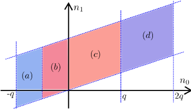
(e) Windows for Seiberg duality on node 3.

(f) $\mathcal{Q}_{(1;3)}$

Figure 4: Left: Windows in the fundamental domain on the $(n_{0},n_{1})$ plane, depending on which kind of mutation one should perform on the CS theories $(\mathcal{Q}_{(0)},\bm{N},\bm{k})$ at a given node $i_{0}$. The windows are bluish when $\theta_{i_{0}-}$ and $\theta_{i_{0}+}$ have opposite signs, and reddish when they have the same sign. Right: Corresponding dual quivers $\mathcal{Q}_{(1;i_{0})}$.

4.2 Dual theories from mutations

Given the technology we have introduced, it is quite easy (with some help from Mathematica) to work out the Seiberg dual Chern-Simons theories. For definiteness we present the results for the theories based on the quivers $\mathcal{Q}_{(1;i_{0})}$, at the first level in the duality tree. In that case the quiver representation $\mathcal{O}_{p}$ for a D2-brane corresponds to a gauge group $U(2)\times U(1)\times U(1)$ and cyclic permutations thereof.

Duality on node 1

Consider mutating the quiver $\mathcal{Q}_{(0)}$ of Figure 2(a) on node $1$, giving rise to the quiver $\mathcal{Q}_{(1;1)}$ of Figure 4(b). The $\theta$ parameters of the fractional D-branes described by the field theories of Table 1 are:

Window $$[y,x] \qquad\theta_{1-}=n_{0}\, \quad\theta_{1+}=3n_{1}-n_{0}\,$$: , (4.12)

Window $$[x,x] \qquad\theta_{1-}=n_{0}\, \quad\theta_{1+}=3n_{1}-n_{0}\,$$: ,

Window $$[z,x] \qquad\theta_{1-}=-2n_{0}+3q\, \quad\theta_{1+}=3n_{1}-n_{0}\,$$: ,

This gives us four windows, denoted $(a)$, $(b)$, $(c)$, $(d)$ in Figure 4(a):

$$(a)\,: \quad\theta_{1-}\leq 0\,,\quad\theta_{1+}\geq 0: -q\leq n_{0}\leq 0\,, \quad 0\leq 3n_{1}-n_{0}\leq 3p-q$$ (4.13)

$$(b)\,: \quad\theta_{1-}\geq 0\,,\quad\theta_{1+}\geq 0: 0\leq n_{0}\leq q\,, \quad 0\leq 3n_{1}-n_{0}\leq 3p-q$$

$$(c)\,: \quad\theta_{1-}\geq 0\,,\quad\theta_{1+}\geq 0: q\leq n_{0}\leq\tfrac{3}{2}q\,, \quad 0\leq 3n_{1}-n_{0}\leq 3p-q$$

$$(d)\,: \quad\theta_{1-}\leq 0\,,\quad\theta_{1+}\geq 0: \tfrac{3}{2}q\leq n_{0}\leq 2q\,, \quad 0\leq 3n_{1}-n_{0}\leq 3p-q$$

The dual $\mathcal{Q}_{(1;1)}$ quiver theory has ranks and CS levels obtained from the mutated dictionaries according to (3.22). In window $(a)$ we have

$$Q^{\vee}_{-}=M_{1;L}^{T}Q^{\vee}_{(y)}=\begin{pmatrix}-1&-\frac{1}{2}&-\frac{1}{8}\\ 1&\frac{3}{2}&\frac{9}{8}\\ 1&-\frac{1}{2}&\frac{1}{8}\end{pmatrix}\,,\qquad Q^{\vee}_{+}=M_{1;R}^{T}Q^{\vee}_{(x)}=\begin{pmatrix}-1&-\frac{1}{2}&-\frac{1}{8}\\ 1&\frac{3}{2}&\frac{9}{8}\\ 1&-\frac{1}{2}&\frac{1}{8}\end{pmatrix}\,.$$ (4.14)

We see that $Q^{\vee}_{-}=Q^{\vee}_{+}$ in this case. In window $(b)$ we have

$$Q^{\vee}_{-}=M_{1;R}^{T}Q^{\vee}_{(x)}\,,\qquad Q^{\vee}_{+}=M_{1;R}^{T}Q^{\vee}_{(x)}$$ (4.15)

so that $Q^{\vee}_{-}=Q^{\vee}_{+}$ again, and it turns out that this dictionary is the same as (4.14) for window $(a)$. Therefore the CS theories in window $(a)$ and $(b)$ are the same. Similarly we find the dictionaries for windows $(c)$

$$Q^{\vee}_{-}=M_{1;R}^{T}Q^{\vee}_{(z)}=\begin{pmatrix}2&-2&\frac{1}{4}\\ -5&\frac{9}{2}&\frac{3}{8}\\ 1&-\frac{1}{2}&\frac{1}{8}\end{pmatrix}\,,\qquad Q^{\vee}_{+}=M_{1;R}^{T}Q^{\vee}_{(x)}=\begin{pmatrix}-1&-\frac{1}{2}&-\frac{1}{8}\\ 1&\frac{3}{2}&\frac{9}{8}\\ 1&-\frac{1}{2}&\frac{1}{8}\end{pmatrix}\,,$$ (4.16)

and for window $(d)$

$$Q^{\vee}_{-}=M_{1;R}^{T}Q^{\vee}_{(z)}=\begin{pmatrix}2&-2&\frac{1}{4}\\ 1&-\frac{3}{2}&\frac{9}{8}\\ -5&\frac{11}{2}&-\frac{5}{8}\end{pmatrix}\,,\qquad Q^{\vee}_{+}=M_{1;R}^{T}Q^{\vee}_{(x)}=\begin{pmatrix}-1&-\frac{1}{2}&-\frac{1}{8}\\ 1&\frac{3}{2}&\frac{9}{8}\\ 1&-\frac{1}{2}&\frac{1}{8}\end{pmatrix}\,,$$ (4.17)

Using the mutated dictionaries in their respective windows of validity, we find the CS quivers theories $(\mathcal{Q}_{(1;1)},\bm{N},\bm{k})$ of Table 2.

$$\qquad\text{Conditions}:\qquad-q\leq n_{0}\leq q\,,\qquad\qquad 0\leq 3n_{1}-n_{0}\leq 3p-q$$

$$\boxed{\text{SD}_{1}(a)\&(b)\,:\,\begin{cases}&\bm{N}\,=\,(2N+p-n_{1},N,N-n_{1})\\ &\bm{k}\,=\,(n_{0}-\frac{3n_{1}}{2},-n_{0}+\frac{3n_{1}}{2}+\frac{3p}{2}-q,-n_{0}+\frac{3n_{1}}{2}-\frac{3p}{2}+q)\end{cases}}$$

$$\qquad\text{Conditions}:\qquad q\leq n_{0}\leq\tfrac{3}{2}q\,,\qquad\qquad 0\leq 3n_{1}-n_{0}\leq 3p-q$$

$$\boxed{\text{SD}_{1}(c)\,:\,\begin{cases}&\bm{N}\,=\,(2N+p-n_{1},N,N-n_{1}+n_{0}-q)\\ &\bm{k}\,=\,(-\frac{n_{0}}{2}-\frac{3n_{1}}{2}+\frac{3q}{2},2n_{0}+\frac{3n_{1}}{2}+\frac{3p}{2}-4q,-n_{0}+\frac{3n_{1}}{2}-\frac{3p}{2}+q)\end{cases}}$$

$$\qquad\text{Conditions}:\qquad\tfrac{3}{2}q\leq n_{0}\leq 2q\,,\qquad\qquad 0\leq 3n_{1}-n_{0}\leq 3p-q$$

$$\boxed{\text{SD}_{1}(d)\,:\,\begin{cases}&\bm{N}\,=\,(2N+p-n_{1}+2n_{0}-3q,N,N-n_{1}+n_{0}-q)\\ &\bm{k}\,=\,(-\frac{n_{0}}{2}-\frac{3n_{1}}{2}+\frac{3q}{2},-n_{0}+\ \frac{3n_{1}}{2}+\frac{3p}{2}+\frac{q}{2},2n_{0}+\frac{3n_{1}}{2}-\frac{3p}{2}-\frac{7q}{2})\end{cases}}$$

Table 2: Seiberg dual CS theories “SD₁” for the quiver $\mathcal{Q}_{(1;1)}$, for any value of $(n_{0},n_{1})\in\Gamma$. The notation SD${}_{i_{0}}$ means that the duality was performed on node $i_{0}$ of the $\mathcal{Q}_{(0)}$ quiver.

Duality on node 2

We should play the same game for each of the nodes of $\mathcal{Q}_{(0)}$. Dualizing on $i_{0}=2$ leads to a subdivision of the fundamental domain into 8 windows, shown in Figure 4(c). The resulting CS quiver theories based on $\mathcal{Q}_{(1,2)}$ are listed in Tables 3 and 4. In this case each of the 8 windows lead to distinct ranks and CS levels.

$$\qquad\text{Conditions}:\qquad-q\leq n_{0}\leq 0\,,\qquad\qquad\tfrac{1}{2}(3p-q)\leq 3n_{1}-n_{0}\leq 3p-q$$

$$\boxed{\text{SD}_{2}(a_{1})\,:\,\begin{cases}&\bm{N}\,=\,(N-n_{0}+n_{1}-p,2N-2n_{0}+3n_{1}-3p+q,N-n_{1})\\ &\bm{k}\,=\,(2n_{0}-\frac{15n_{1}}{2}+\frac{9p}{2}-\frac{3q}{2},-\frac{n_{0}}{2}+3n_{1}-\frac{3p}{2}+q,-n_{0}+\frac{3n_{1}}{2}-\frac{3\ p}{2}-\frac{q}{2})\end{cases}}$$

$$\qquad\text{Conditions}:\qquad-q\leq n_{0}\leq 0\,,\qquad\qquad 0\leq 3n_{1}-n_{0}\leq\tfrac{1}{2}(3p-q)$$

$$\boxed{\text{SD}_{2}(b_{1})\,:\,\begin{cases}&\bm{N}\,=\,(N-n_{0}+n_{1}-p,2N-3n_{1},N-n_{1})\\ &\bm{k}\,=\,(\frac{3n_{1}}{2}-n_{0},-\frac{n_{0}}{2}+3n_{1}-\frac{3p}{2}+q,2n_{0}-\frac{15n_{1}}{2}+3p-2q)\end{cases}}$$

$$\qquad\text{Conditions}:\qquad 0\leq n_{0}\leq\tfrac{1}{2}q\,,\qquad\qquad\tfrac{1}{2}(3p-q)\leq 3n_{1}-n_{0}\leq 3p-q$$

$$\boxed{\text{SD}_{2}(a_{2})\,:\,\begin{cases}&\bm{N}\,=\,(N+n_{1}-p,2N-2n_{0}+3n_{1}-3p+q,N-n_{1})\\ &\bm{k}\,=\,(2n_{0}-\frac{15n_{1}}{2}+\frac{9p}{2}-\frac{3q}{2},-2n_{0}+3n_{1}-\frac{3p}{2}+q,2n_{0}+\frac{3n_{1}}{2}-\frac{3p}{2}-\frac{q}{2})\end{cases}}$$

$$\qquad\text{Conditions}:\qquad 0\leq n_{0}\leq\tfrac{1}{2}q\,,\qquad\qquad 0\leq 3n_{1}-n_{0}\leq\tfrac{1}{2}(3p-q)$$

$$\boxed{\text{SD}_{2}(b_{2})\,:\,\begin{cases}&\bm{N}\,=\,(N+n_{1}-p,2N-3n_{1},N-n_{1})\\ &\bm{k}\,=\,(\frac{3n_{1}}{2}-n_{0},-2n_{0}+3n_{1}-\frac{3p}{2}+q,5n_{0}-\frac{15n_{1}}{2}+3p-2q)\end{cases}}$$

Table 3: Seiberg dual CS theories “SD₂” for the quiver $\mathcal{Q}_{(1;2)}$.

$$\qquad\text{Conditions}:\qquad\tfrac{1}{2}q\leq n_{0}\leq q\,,\qquad\qquad\tfrac{1}{2}(3p-q)\leq 3n_{1}-n_{0}\leq 3p-q$$

$$\boxed{\text{SD}_{2}(c_{2})\,:\,\begin{cases}&\bm{N}\,=\,(N+n_{1}-p,2N+3n_{1}-3p,N-n_{1})\\ &\bm{k}\,=\,(5n_{0}-\frac{15n_{1}}{2}+\frac{9p}{2}-3q,-2n_{0}+3n_{1}-\frac{3p}{2}+q,-n_{0}+\frac{3n_{1}}{2}-\frac{3p}{2}+q)\end{cases}}$$

$$\qquad\text{Conditions}:\qquad\tfrac{1}{2}q\leq n_{0}\leq q\,,\qquad\qquad 0\leq 3n_{1}-n_{0}\leq\tfrac{1}{2}(3p-q)$$

$$\boxed{\text{SD}_{2}(d_{2})\,:\,\begin{cases}&\bm{N}\,=\,(N+n_{1}-p,2N+2n_{0}-3n_{1}-q,N-n_{1})\\ &\bm{k}\,=\,(2n_{0}+\frac{3n_{1}}{2}-\frac{3q}{2},-2n_{0}+3n_{1}-\frac{3p}{2}+q,2n_{0}-\frac{15n_{1}}{2}+3p-\frac{q}{2})\end{cases}}$$

$$\qquad\text{Conditions}:\qquad q\leq n_{0}\leq 2q\,,\qquad\qquad\tfrac{1}{2}(3p-q)\leq 3n_{1}-n_{0}\leq 3p-q$$

$$\boxed{\text{SD}_{2}(c_{1})\,:\,\begin{cases}&\bm{N}\,=\,(N+n_{1}-p,2N+3n_{1}-3p,N+n_{0}-n_{1}-q)\\ &\bm{k}\,=\,(2n_{0}-\frac{15n_{1}}{2}+\frac{9p}{2},-\frac{n_{0}}{2}+3n_{1}-\frac{3p}{2}-\frac{q}{2},-n_{0}+\frac{3n_{1}}{2}-\frac{3p}{2}+q)\end{cases}}$$

$$\qquad\text{Conditions}:\qquad q\leq n_{0}\leq 2q\,,\qquad\qquad 0\leq 3n_{1}-n_{0}\leq\tfrac{1}{2}(3p-q)$$

$$\boxed{\text{SD}_{2}(d_{1})\,:\,\begin{cases}&\bm{N}\,=\,(N+n_{1}-p,2N+2n_{0}-3n_{1}-q,N+n_{0}-n_{1}-q)\\ &\bm{k}\,=\,(-n_{0}+\frac{3n_{1}}{2}+\frac{3q}{2},-\frac{n_{0}}{2}+3n_{1}-\frac{3p}{2}-\frac{q}{2},2n_{0}-\frac{15n_{1}}{2}+3p-\frac{q}{2})\end{cases}}$$

Table 4: Seiberg dual CS theories “SD₂”, continued.

Duality on node 3

Dualizing on node 3 we find a pattern similar to the node 1 case, to which it is related by a $\mathbb{Z}_{2}$ operation (which is CP in the original $\mathcal{Q}_{(0)}$ quiver). We have four windows in Figure 4(e) and it turns out there are only three distinct pair of dictionaries. The dual theories are the $\mathcal{Q}_{(1;3)}$ quiver with the ranks and CS levels of Table 5.

$$\qquad\text{Conditions}:\qquad-q\leq n_{0}\leq-\tfrac{1}{2}q\,,\qquad\qquad 0\leq 3n_{1}-n_{0}\leq 3p-q$$

$$\boxed{\text{SD}_{3}(a)\,:\,\begin{cases}&\bm{N}\,=\,(N-n_{0}+n_{1}-p,N,2N-2n_{0}+n_{1}-q)\\ &\bm{k}\,=\,(2n_{0}+\frac{3n_{1}}{2}+\frac{3q}{2},-n_{0}+\frac{3n_{1}}{2}-3p+\frac{q}{2},-\frac{n_{0}}{2}-\frac{3n_{1}}{2}+\frac{3p}{2}-q)\end{cases}}$$

$$\qquad\text{Conditions}:\qquad-\tfrac{1}{2}q\leq n_{0}\leq 0\,,\qquad\qquad 0\leq 3n_{1}-n_{0}\leq 3p-q$$

$$\boxed{\text{SD}_{3}(b)\,:\,\begin{cases}&\bm{N}\,=\,(N-n_{0}+n_{1}-p,N,2N+n_{1})\\ &\bm{k}\,=\,(\frac{3n_{1}}{2}-n_{0},2n_{0}+\frac{3n_{1}}{2}-3p+2q,-\frac{n_{0}}{2}-\frac{3n_{1}}{2}+\frac{3p}{2}-q)\end{cases}}$$

$$\qquad\text{Conditions}:\qquad 0\leq n_{0}\leq 2q\,,\qquad\qquad 0\leq 3n_{1}-n_{0}\leq 3p-q$$

$$\boxed{\text{SD}_{3}(c)\&(d)\,:\,\begin{cases}&\bm{N}\,=\,(N+n_{1}-p,N,2N+n_{1})\\ &\bm{k}\,=\,(\frac{3n_{1}}{2}-n_{0},-n_{0}+\frac{3n_{1}}{2}-3p+2q,n_{0}-\frac{3n_{1}}{2}+\frac{3p}{2}-q)\end{cases}}$$

Table 5: Seiberg dual CS theories “SD₃” for the quiver $\mathcal{Q}_{(1;3)}$.

4.3 Consistency checks and remarks

We have just presented the complete list of the Chern-Simons quiver theories $(\mathcal{Q}_{(1;i_{0})},\bm{N},\bm{k})$ obtained by doing one Seiberg duality on the CS theories of Table 1. At any fixed $(n_{0},n_{1})$ the corresponding $\mathcal{Q}_{(0)}$-quiver theory has three distinct Seiberg dual theories. For instance, the dual theories to the torsionless point $(n_{0},n_{1})=(0,0)$ are

$$\mathcal{Q}_{(1;1)} :\,\qquad U(2N+p)_{0}\times U(N)_{\frac{3}{2}p-q}\times U(N)_{-\frac{3}{2}p+q}\,,$$ (4.18)

$$\mathcal{Q}_{(1;2)} :\,\qquad U(N-p)_{0}\times U(2N)_{-\frac{3}{2}p+q}\times U(N)_{3p-2q}\,,$$

$$\mathcal{Q}_{(1;3)} :\,\qquad U(N-p)_{0}\times U(N)_{-3p+2q}\times U(2N)_{\frac{3}{2}p-q}\,.$$

The semi-classical moduli space can be analyzed similarly to [11]. Remark that the first theory in (4.18) has naively a larger Coulomb branch than the one of the original theory, but in this case the semi-classical brane derivation we performed actually fails: It was shown by Aharony [50] that the Seiberg dual in that case with $k_{i_{0}}=0$ involves extra singlets and additional couplings to monopoles, which should conspire to give the correct matching of moduli spaces.

For generic $(n_{0},n_{1})$ it is obvious that the geometric branch (see section 3.1) of the semi-classical moduli space of $(\mathcal{Q},\bm{N},\bm{k})$ reproduces the type IIA geometry. This is true by construction: We should compute the parameters $\bm{k_{\pm}}=\pm\bm{\theta}_{\pm}$ from the quiver data and use the dictionaries $Q^{\vee}_{\pm}$ to find the IIA resolutions parameters (3.13), but this is just inverting the steps we followed to find the field theories in the first place.

A better consistency check is that the Seiberg dual field theories reproduce the periodicities $(n_{0},n_{1})\sim(n_{0}+3q,n_{1}+q)$ and $(n_{0},n_{1})\sim(n_{0}+q,n_{1}+p)$ of the torsion group (4.9). This is indeed the case. The field theories on the external boundaries of the various windows in Figures 4(a), 4(c), 4(e) are identified according to

$$\delta{(n_{0},n_{1})}=(3q,q) :\quad\text{SD}_{i_{0}}\rightarrow\text{SD}_{i_{0}}\,,$$ (4.19)

$$\delta{(n_{0},n_{1})}=(q,p) :\quad\text{SD}_{i_{0}}\rightarrow\text{SD}_{i_{0}-1}\,,$$

meaning that the periodicity $(3q,q)$ sends a theory in the family $\text{SD}_{1}$ to another identical one in the same family, while the periodicity $(q,p)$ sends a theory in $\text{SD}_{i_{0}}$ to one in another family $\text{SD}_{i_{0}-1}$. In other words, the first periodicity is apparent inside any of the three families of $\mathcal{Q}_{(1;i_{0})}$-quivers while the second one holds because of Seiberg dualities.

4.4 Monopole operators and matching the chiral ring

Beyond the semi-classical analysis of the moduli space, which reproduces the IIA geometry, we can check our Seiberg dual quivers by seeing whether the quantum chiral rings of dual theories coincide, as they should. In particular the chiral ring should reproduce the CY₄ cone probed by the M2-branes according to the construction (3.8). The analysis we perform here is “pseudo-Abelian”: the monopole operators we construct are best thought of as functions on the Coulomb branch. A comprehensive analysis of the monopoles in the non-Abelian theory (for instance along the lines of [52]) would require more sophisticated tools, and we leave it for future work.

Some useful facts about the relevant “diagonal” monopole operators are collected in Appendix D.

Toric quiver monopoles

The gauge invariant operators generating the chiral ring (or rather the subspace of it corresponding to (3.8)) of the toric CS quiver theories of [11] are:

$$[y,x]\;: \quad\bm{a}_{(3)}=XYZ\;,\quad\bm{b}_{(q)}=TX^{-n_{0}}Z^{q+n_{0}}\;,\quad\bm{c}_{(3p-q)}=\tilde{T}Y^{3n_{1}-n_{0}}Z^{3p-q-3n_{1}+n_{0}}\,,$$ (4.20)

$$[x,x]\;: \quad\bm{a}_{(3)}=XYZ\;,\quad\bm{b}_{(q)}=TY^{n_{0}}Z^{q-n_{0}}\;,\quad\bm{c}_{(3p-q)}=\tilde{T}Y^{3n_{1}-n_{0}}Z^{3p-q-3n_{1}+n_{0}}\,,$$

$$[z,x]\;: \quad\bm{a}_{(3)}=XYZ\;,\quad\bm{b}_{(q)}=TX^{-q+n_{0}}Y^{2q-n_{0}}\;,\quad\bm{c}_{(3p-q)}=\tilde{T}Y^{3n_{1}-n_{0}}Z^{3p-q-3n_{1}+n_{0}}\,.$$

The subscript corresponds to the number of symmetrized $SU(3)$ indices: The operator $\bm{a}_{3}$ transforms in the $\text{Sym}^{3}\,\bm{3}=\bm{10}$, etc. We stress again that the operators (4.20) should be thought of as regular functions on the Coulomb branch. On the other hand at the origin of the Coulomb branch (where the CFT lives) we should contract the indices according to the non-Abelian representations of $T$, $\tilde{T}$ (see Appendix D), and looking at all possible gauge invariant operators in the CFT one finds that the diagonal monopole operators fall in larger $SU(3)$ representations than the ones apparent in (4.20).. We are left to assume that these extra operators fail to be chiral due to non-perturbative effects, but this issue would deserve a more serious study. In any case the operators (4.20) together with the quantum relation

$$\bm{b}_{(q)}\,\bm{c}_{(3p-q)}\,\sim\,(\bm{a}_{(3)})^{p}$$ (4.21)

reproduce the coordinate ring of the CY₄ cone $C(Y^{p,q}(\mathbb{C}\mathbb{P}^{2}))$.

Monopoles in Seiberg dual quivers

For definiteness let us focus on the first of the 14 Seiberg dual theories listed in Tables 2 to 5, which we called “$\text{SD}_{1}(a)\&(b)$”. This is the quiver of Figure 4(b) with gauge group and CS levels

$$U(2N+p-n_{1})_{n_{0}-\frac{3}{2}n_{1}}\times U(N)_{-n_{0}+\frac{3}{2}n_{1}+\frac{3}{2}p-q}\times U(N-n_{1})_{-n_{0}+\frac{3}{2}n_{1}-\frac{3}{2}p+q}$$ (4.22)

Let us denote by $g_{i}$ the electric charge under the diagonal $U(1)_{i}\subset U(N_{i})$. The electric and global charges of the bifundamental fields and of the bare monopoles $T$ and $\tilde{T}$ are:

$$\begin{array}[]{c|ccc|c|c}&X^{a}&Y^{a}&Z_{ab}&T&\tilde{T}\\ \hline\cr g_{1}&-1&1&0&2[n_{0}]&2[-n_{0}+3n_{1}]\\ g_{2}&0&-1&1&-n_{0}-q&n_{0}-3n_{1}-3p+q\\ g_{3}&1&0&-1&-n_{0}+q&n_{0}-3n_{1}+3p-q\\ \hline\cr\rule[-4.30554pt]{0.0pt}{15.0694pt}R&2-R_{Y}-R_{Z}&R_{Y}&R_{Z}&R_{T}&R_{T}\\ SU(3)&\mathbf{\bar{3}}&\mathbf{\bar{3}}&\mathbf{6}&\mathbf{1}&\mathbf{1}\\ U(1)_{M}&0&0&0&1&-1\end{array}$$ (4.23)

where we denoted $R_{X}=R[X]$ the R-charge of any field $X$, and

$$R_{T}=-2p+3n_{1}-3n_{1}R_{Y}+\frac{3}{2}(p-n_{1})R_{Z}\,.$$ (4.24)

From (4.23) we find the gauge invariant operators

$$\bm{a}_{(3)}=XYZ\;,\qquad\bm{b}_{(q)}=TX^{q-n_{0}}Y^{q+n_{0}}\;,\qquad\bm{c}_{(3p-q)}=\tilde{T}X^{3p-q+n_{0}-3n_{1}}Z^{3p-q+3n_{1}-n_{0}}\,.$$ (4.25)

The operators $\bm{b}$ and $\bm{c}$ are regular functions (all the powers in the expressions (4.25) are positives) if and only if

$$-q\leq n_{0}\leq q\,,\qquad-(3p-q)\leq 3n_{1}-n_{0}\leq 3p-q$$ (4.26)

This agrees with the condition for the $\text{SD}_{1}(a)\&(b)$ theory to be valid, and in fact it cuts out a window in the $(n_{0},n_{1})$ plane which is twice larger than windows $(a)\&(c)$ of Figure 4(a).

The operators (4.25) have the correct R-charges to allow the quantum relation (4.21). They also transform in the same $SU(3)$ representation as the operators (4.20) of the original theory, namely $\text{Sym}^{q}\bm{3}$ and $\text{Sym}^{3p-q}\bm{3}$. To understand this we have to deal with the fact that the theory on the Coulomb branch is not Abelian anymore. The “pseudo-Abelian” theory (one single D2-brane) is a $U(2)\times U(1)\times U(1)$ theory with CS levels $\bm{k}_{-}$ or $\bm{k}_{+}$ for $\sigma<0$ or $\sigma>0$, respectively. Consider the $\sigma<0$ case, where the bare monopole is $T$ transforming in the $[n_{0},n_{0}]$ of $U(2)$ and with charge $-n_{0}-q$ and $-n_{0}+q$ under the $U(1)$’s of the second and third node. Let $Y\cdot X$ denote the contraction of $Y$ and $X$ on their $U(2)$ indices. Due to the superpotential (4.8) $Y\cdot X$ transforms in the $\mathbf{3}$ of $SU(3)$. We have

$$\bm{b}_{(q)}=\begin{cases}T(Y\cdot X)^{q}\,,&\qquad\text{if}\;n_{0}=0\\ T\cdot Y^{2n_{0}}(Y\cdot X)^{q-n_{0}}\,,&\qquad\text{if}\;n_{0}>0\\ T\cdot X^{-2n_{0}}(Y\cdot X)^{q+n_{0}}\,,&\qquad\text{if}\;n_{0}<0\end{cases}$$ (4.27)

In the first case we obviously have the correct $SU(3)$ representation. In the second case the contraction $T\cdot Y^{2n_{0}}$ gives the representation $\text{Sym}^{n_{0}}\bm{3}$ (using $\bm{\bar{3}}\otimes_{A}\bm{\bar{3}}=\mathbf{3}$ and so forth), and thus the operator $T\cdot Y^{2n_{0}}(Y\cdot X)^{q-n_{0}}$ lies in the

$$\text{Sym}^{n_{0}}\bm{3}\,\otimes\,\text{Sym}^{q-n_{0}}\bm{3}\,\supset\,\text{Sym}^{q}\bm{3},,$$ (4.28)

which contains the expected representation $\text{Sym}^{q}\bm{3}$. We can similarly analyze the third case in (4.27), and the monopoles $\bm{c}_{(3p-q)}$ at $\sigma>0$. The extra $SU(3)$ representations in (4.28) are puzzling. For lack of better tools, we are left to conjecture that the corresponding operators are set to zero in the quantum chiral ring. At the torsionless point $n_{0}=n_{1}=0$ the monopole operators match across Seiberg duality without extra assumption.

A similar analysis can be performed in any of the 14 windows of Figure 4, with similar conclusions.

5 Remark on brane charge and CS quivers dual to massive IIA geometries

This section lies outside the main line of development of the paper. It aims to clarify a point in the treatment of brane charge of [11], and it allows to generalize the construction of [11] to CS quivers with $\sum_{i}k_{i}\neq 0$, corresponding to the presence of D8-brane charge in type IIA.

The quantities that we loosely referred to as “brane charges” in this work are quantized and conserved charges corresponding to either quantized RR flux or explicit D-brane sources (the latter sourcing the former). In [11] we identified such brane charges with Page charges [53], which is a concept mostly relevant to the supergravity limit of string theory. Consider a type IIA Dp-brane $\mathsf{E}^{\vee}$ wrapped on some $(p-2)$-cycle $S\subset\tilde{Y}$ with some worlvolume flux $F_{wv}$ turned on. The brane charges of such a source can be read from its Wess-Zumino action,

$$S_{WZ}=\tau_{p}\int_{\mathbb{R}^{2,1}\times S}C^{(P)}Q(\mathsf{E}^{\vee})\,,$$ (5.1)

where $C^{(P)}$ is defined in term of the ordinary RR potential $C$ (a polyform) as $C^{(P)}=C\wedge e^{B}$ with $B$ the background $B$-field pulled-back on the D-brane [54]. We restrict ourselves to cases where $B$ is flat, and in such a situation this $C^{(P)}$ is the potential for the Page currents

$$F^{(P)}=Fe^{B}\,.$$ (5.2)

The point of this distinction is that the Page charge is sourced only by the D-brane and its worlvolume flux, and therefore they are properly quantized; on the other hand they are not invariant under large gauge tranformations $B\rightarrow B+\Lambda$, $F_{wv}\rightarrow F_{wv}-\Lambda$. The quantity $Q(\mathsf{E}^{\vee})$ in (5.1) is by definition the (Page) brane charge. It is given by [56]

$$Q(E^{\vee})=ch(E^{\vee})\sqrt{\frac{\hat{A}(TS)}{\hat{A}(NS)}}\,,$$ (5.3)

with $\hat{A}$ the A-roof characteristic class, here for the tangent and normal bundles to $S$. This brane charge is a K-theory class, and indeed K-theory is the natural concept of charge for the B-brane category [57, 37]. In [11] and in this work, we just took $Q(E^{\vee})=ch(E^{\vee})$ as our working definition of D-brane charge, but in general we should use the exact formula (5.3). The gravitational correction in (5.3) translates to small corrections to the brane charge dictionaries $Q^{\vee}$. This does not affect the results of [11], where these corrections where ignored in a consistent way.

These considerations are however important if we want to generalize the string theory derivations of CS quivers of [11] to cases with $\sum_{i}r_{i}k_{i}\neq 0$. This corresponds to having D8-brane charge (in the guise of $F_{0}$ flux) in the type IIA dual [58, 59]: the fluxes in (3.11) become

$$\bm{Q}_{\text{flux}}\,=\,\left(-Q_{4}\,|\,Q_{6;\,\alpha}\,|\,Q_{8}\right)\,,\\$$ (5.4)

It is possible to work out the effect of $Q_{8}=F_{0}\neq 0$ on the derivation of [11], reviewed in section 4.1. Accounting for the gravitational correction in (5.3), the brane charges dictionaries (4.11) become

$$Q^{\vee}_{(x)}=\begin{pmatrix}1&\frac{1}{2}&\frac{1}{4}\\ -2&0&\frac{1}{2}\\ 1&-\frac{1}{2}&\frac{1}{4}\end{pmatrix}\;,\quad Q^{\vee}_{(y)}=\begin{pmatrix}1&\frac{1}{2}&\frac{1}{4}\\ 1&\frac{3}{2}&\frac{5}{4}\\ -2&-2&-\frac{1}{2}\end{pmatrix}\;,\quad Q^{\vee}_{(z)}=\begin{pmatrix}-2&2&-\frac{1}{2}\\ 1&-\frac{3}{2}&\frac{5}{4}\\ 1&-\frac{1}{2}&\frac{1}{4}\end{pmatrix}\;,$$ (5.5)

and the sources and fluxes (4.10) are shifted to

$$\bm{Q}_{\text{flux},-} \equiv\,\left(-n_{0}+\tfrac{1}{2}q-\frac{1}{4}F_{0}\,|\,-q\,|\,F_{0}\right)\,,$$ (5.6)

$$\bm{Q}_{\text{source}} \equiv\,\left(-p\,|\,n_{1}-\tfrac{1}{2}p\,|\,N-\tfrac{1}{4}p\right)\,.$$

Running our algorithm, this gives the same results as in Table 1, except that the Chern-Simons levels are shifted to

$$\bm{k}\rightarrow\bm{k}_{\,(\text{Table \ref{tab: three theories dP0 toric})}}+(0,F_{0},0)\,,$$ (5.7)

and therefore $\sum_{i}k_{i}=F_{0}$.

These Chern-Simons quiver theories should be dual to the massive type IIA $AdS_{4}$ solutions of [60]. We can thus provide a precise map between the six field theory parameters $(\bm{N},\bm{k})$ and the supergravity parameters of that paper. It would be interesting to see whether one can perform non-trivial tests of this duality that would be sensitive to the finer details of this map.

6 Conclusions

We have shown that for Chern-Simons quivers realized as fractional brane quivers in type IIA string theory, Seiberg-like dualities are easily found by changing the fractional brane basis, much like what happens for D3-brane quiver theories. In particular, we concentrated on maximally chiral quivers for D-branes at CY₃ cones with a single exceptional divisor. It would be worthwhile but technically challenging to generalize the argument of this paper to completely general $CY_{3}$ quivers. In any case the subclass we analyzed contains the newly discovered “chiral” Seiberg-like dualities of [14].

We believe our approach to be quite powerful, as demonstrated in the example of section 4: All the computations of mutated dictionaries and dual CS quiver gauge theories are easily done on a computer, for arbitrarily complicated examples. Indeed some more general examples of mutated dictionaries have already appeared in the related work [12].

There are a number of issues and open questions that we did not address. We should stress that the B-brane pictures is not sensible to the finer details of 3d Seiberg duality. It does not see the parity anomaly in the Abelian sector of chiral quivers, which so far has to be fixed “by hand” [11]. Moreover, it cannot account for the extra singlet fields (dual to monopole operators) which appear in 3d Seiberg duality when some effective CS level vanishes [50, 14]. These shortcoming are expected since the B-model is a $g_{s}=0$ approximation of string theory, and we should not expect too much from B-branes. Seiberg duality for chiral quivers should thus also be further studied with field theory methods.

Originally, this work was motivated by a desire to understand 3d Seiberg duality in a manner conceptually similar to the Berenstein-Douglas approach to Seiberg duality [24]. Such point of view was also recently taken in [61]. In that respect we did not reach our goal, because we could not abstract the discussion from the underlying D-branes. It would be interesting to pursue this avenue. A possibility would be to formalize $\mathcal{N}=2$ Chern-Simons quiver theories as families of “decorated” quiver representations, similar (but different) from those studied in [26], and try to understand how quiver mutation induces an action on such objects.

Finally, we believe mutations of fractional branes should be studied again in their own right by physicists. Previous work on D-branes on Fano varieties [31, 16, 32, 40] focussed on complete strongly exceptional collections, but it seems that the more general notion one should use is the one of tilting collection, which is slightly weaker. We conjectured in section 2.4 that there exists a good notion of mutation of a tilting collection which gives another tilting collection, but this certainly calls for a proof. Indeed we did not even define the correct mutation operation in term of sheaves, but only in term of their charges. One should also study more seriously the relation between tilting collections on $\tilde{B}_{4}$ and on its canonical bundle $\tilde{Y}=\mathcal{O}_{\tilde{B}_{4}}(K)$. We hope that continuing progress in the mathematical literature on the subject will allow to address those questions rigorously.

Appendix A More on quivers and Seiberg duality

A category is a class of objects and a class of map between them, called morphisms, which can be composed naturally. There are all sorts of categories satisfying more specialized axioms. A simple kind of categories are Abelian categories, which are such that every morphism has a kernel and cokernel (in the appropriate abstract sense of homological algebra). For every Abelian category $\mathsf{A}$ we can construct a derived category $D(\mathsf{A})$ whose objects are chain complexes of the objects in $\mathsf{A}$ (up to some equivalence relations); see [37] for a physics-oriented introduction.

In the following we review some elementary facts about the category of quiver representations for $CY_{3}$ quivers, and we review the Berenstein-Douglas [24] understanding of Seiberg duality as an equivalence of derived category of quiver representations. These facts are reviewed for completeness: they are not essential to the main flow of ideas of the paper, but they provide its conceptual context.

We always work over the field $\mathbb{C}$.

A.1 Quivers, path algebra and $\mathcal{A}$-modules

Quivers and their representations.

Formally, a quiver $\mathcal{Q}=(Q_{0},Q_{1},s,t)$ is a set of nodes $Q_{0}$, a set of arrows $Q_{1}$ between the nodes, and two functions

$$s:Q_{1}\rightarrow Q_{0}\,,\qquad t:Q_{1}\rightarrow Q_{0}$$ (A.1)

such that $s(a_{ij})=i$ (the “source” node) and $t(a_{ij})=j$ (the “target” node). A path from $i$ to $j$, $p:i\rightarrow j$, is a sequence of arrows

$$p=a_{1}a_{2}\cdots a_{p}\quad\qquad\text{such that}\quad t(a_{1})=s(a_{2})\,,\;\cdots,\;t(a_{p-1})=s(a_{p})\,.$$ (A.2)

and with $s(a_{1})=i$, $t(a_{p})=j$. A quiver representation $X=(V_{i},X_{a})$ is a choice of vector space $V_{i}$ for each node and a linear map $X_{a}$ for each arrow. A morphism $\phi$ between two quiver representations $X$, $X^{\prime}$ is a set of linear maps $\phi_{i}:V_{i}\rightarrow V^{\prime}_{i}$ such that $\phi_{i}X^{\prime}_{a}=X_{a}\phi_{j}$ for any $a:i\rightarrow j$. For a quiver with relations the maps $X_{a}$ must also satisfy the relations. Two representations are identified if there exist an isomorphism (invertible morphism) between them. Quiver representations and their morphisms form the category of quiver representations, $\mathcal{Q}-\mathrm{rep}$ for short. Moreover $\mathcal{Q}-\mathrm{rep}$ is an Abelian category, rather obviously since the morphisms are linear maps.

Path algebra.

Recall that an algebra is a vector space equipped with a multiplication (not necessarily commutative). The unconstrained path algebra $\mathbb{C}\mathcal{Q}$ of a quiver $\mathcal{Q}$ is the algebra generated by all the possible paths in the quiver, with the multiplication given by the concatenation of paths, namely $a\cdot b=ab$ if $t(a)=s(b)$, and zero otherwise. For each vertex we define a trivial path $e_{i}$ satisfying $e_{i}e_{j}=\delta_{ij}e_{i}$. They act as a projectors and provide an identity element $1=\sum_{i}e_{i}$ in $\mathbb{C}\mathcal{Q}$. For a quiver with superpotential, the path algebra $\mathcal{A}$ is the algebra $\mathbb{C}\mathcal{Q}$ modulo the relations (2.2),

$$\mathcal{A}\equiv\mathbb{C}\mathcal{Q}/(\partial W)\,,$$ (A.3)

with $(\partial W)$ the ideal of $\mathbb{C}\mathcal{Q}$ generated by (2.2).

Modules.

Given any ring $R$, a (right) R-module $M$ is an abelian group $M$ together with a (right) action of $R$, $R:M\times R\rightarrow M$ acting just like a scalar multiplication on a vector space. Morphisms between modules are homomorphisms, $\phi:M\rightarrow M^{\prime}$ such that $\forall m,n\in M$ and $r,s\in R$, $\phi(mr+ns)=\phi(m)r+\phi(n)s\in M^{\prime}$. The modules and morphism over a given ring $R$ form the category $R-\mathrm{mod}$.

A module $M$ is a submodule of $M^{\prime}$ if there exist an injective morphism $\phi:M\rightarrow M^{\prime}$. The dimension of a module $M$ is its dimension as an Abelian group.

A free $R$-module is a module which has a basis (a generating linearly independent set); free modules are what come closest to vector spaces.

A projective $R$-module is a module which is the summand of a free module. In other words, the $R$-module $M$ is projective if there exists an $R$-module $N$ such that $M\oplus N$ is free.

A simple $R$-module is a module which has no proper submodule (no submodule other than itself and the trivial one).

$\mathcal{A}$-modules and $\mathcal{Q}$-representations.

In particular, we can consider $\mathcal{A}$-modules. A standard result is that there exist an equivalence of categories

$$\mathcal{A}-\mathrm{mod}\cong\mathcal{Q}-\mathrm{rep}\,.$$ (A.4)

The equivalence is given by the following maps. For any quiver representation $X=(V_{i},X_{a})$, we define a (right) module $\mathcal{X}$ as the abelian group $\mathcal{X}=\oplus_{i}V_{i}$, with the (right) action of the paths in $\mathcal{A}$ on $\mathcal{X}$ given by

$$x\,a_{1}\cdots a_{p} \;=\;x\,\pi_{s(a_{1})}X_{a_{1}}\cdots X_{a_{p}}\iota_{t(p)}\,,$$ (A.5)

$$x\,e_{i} \;=\;x\,\pi_{i}\iota_{i}\,,$$

$\forall\,x\in\mathcal{X}$, with $\iota_{i}$ and $\pi_{i}$ the inclusion and projection maps $V_{i}\stackrel{{\scriptstyle\iota_{i}}}{{\rightarrow}}\mathcal{X}\stackrel{{\scriptstyle\pi_{i}}}{{\rightarrow}}V_{i}$. In the other direction, for any $\mathcal{A}$-module $\mathcal{X}$, we have a representation $X=(V_{i},X_{a})$ with

$$V_{i} \;=\;\mathcal{X}e_{i}\,,$$ (A.6)

$$xX_{a} \;=\;xa\,,$$

according to the way $a\in\mathcal{A}$ was represented on $\mathcal{X}$. Hence we can talk interchangeably about quiver representation or $\mathcal{A}$-modules, but sometimes one or the other language is more convenient. The dimension vector $\bm{N}$ of a $\mathcal{A}$-module is defined as the $\bm{N}$ of the associated $\mathcal{Q}$-representation. Note that two modules $M$, $N$ are the same if there is an isomorphism between them, by definition, and thus an $\mathcal{A}$-module of dimension $\bm{N}$ corresponds to the gauge orbit of a particular F-term solution in a supersymmetric quiver theory $(\mathcal{Q},\bm{N})$.

A.2 Seiberg duality as a tilting equivalence

Consider a $CY_{3}$ quiver $\mathcal{Q}$ and its path algebra $\mathcal{A}$. Of particular interest are the simple $\mathcal{A}$-modules, because they correspond to “single brane” states. To each node of the quiver we associate a simple module $e_{i}$ and a projective module $P_{i}$. The module $e_{i}$ is the quiver representation with $V_{j}=\delta_{ij}\mathbb{C}$, and correspond to a fractional brane. On the other hand $P_{i}$ is the $\mathcal{A}$-module consisting of all paths ending at node $i$:

$$P_{i}=\mathcal{A}e_{i}\,.$$ (A.7)

These right $\mathcal{A}$-modules are projective since $\oplus_{i}P_{i}=\mathcal{A}$, and we have the identity

$$\mathcal{A}=\text{End}(\oplus_{i}P_{i})^{op}\,,$$ (A.8)

where ^op corresponds to reversing all the arrows in a path algebra. Now, consider going to the derived category of $\mathcal{A}$-modules, $D(\mathcal{A}-\text{mod})$; the image of $P_{i}$ in $D(\mathcal{A}-\text{mod})$ is the single entry complex $P_{i}\equiv 0\rightarrow P_{i}\rightarrow 0$ in position $0$. The objects $P_{i}$ form a tilting collection in the derived category, meaning that they satisfy

$$\text{Ext}^{q}(P_{i},P_{j})=0\,\qquad\qquad\forall q>0\,$$ (A.9)

and generate the full category $D(\mathcal{A}-\text{mod})$. If we have any tilting collection $\{P_{i}^{\prime}\}$ in $D(\mathcal{A}-\text{mod})$, we can define a path algebra

$$\mathcal{A}^{\prime}=\text{End}(\oplus_{i}P^{\prime}_{i})^{op}\,,$$ (A.10)

and therefore a quiver $\mathcal{Q}^{\prime}$. One says that there exists a tilting equivalence between $\mathcal{Q}$ and $\mathcal{Q}^{\prime}$. By Rickard’s theorem [62], any tilting equivalence is an equivalence of derived categories

$$D(\mathcal{A})\cong D(\mathcal{A}^{\prime})\,$$ (A.11)

(and conversely any derived category equivalence can be realized as a tilting equivalence). The proposal of [24] is that Seiberg duality for quivers is such a tilting equivalence. In [63] it was shown that the notion of “doing Seiberg duality at node $i_{0}\in Q_{0}$” is realized by taking the following tilting collections:

$$P^{\prime}_{i}=P_{i}\,\quad\text{if}\;i\neq i_{0}\,,\qquad P_{i}^{\prime}=\left(0\longrightarrow\oplus_{j\in I_{L}}P_{j}\stackrel{{\scriptstyle(a_{ji_{0}})}}{{\longrightarrow}}P_{i_{0}}\longrightarrow 0\right)\,,$$ (A.12)

where $I_{L}\subset Q_{0}$ is the set of nodes connected to $i_{0}$ by ingoing arrows, and the first non-trivial entry in the complex $P_{i}^{\prime}$ is at position $0$. This construction corresponds to the left mutation of quiver representations discussed in the main text, while a similar tilting collection can be constructed for right mutations. Indeed, this construction is also completely parallel to the mutations on the sheaves $E_{i}$ of (2.31), with $P_{i}\sim E_{i}$.

Appendix B More on B-branes and quivers

The relation between a conical CY₃ $Y$ and a quiver $\mathcal{Q}$ can be summarized in a single line,

$$D(\text{Coh}\,\tilde{Y})\cong D(\mathcal{A}_{\mathcal{Q}}\text{-mod})\,,$$ (B.1)

namely it is a derived category equivalence similar to the one for quivers reviewed in the last Appendix. $\text{Coh}\,\tilde{Y}$ is the Abelian category of coherent sheaves on $\tilde{Y}$. In more physical terms, $D(\text{Coh}\,\tilde{Y})$ is the category of B-branes, the boundary states in the topological B-model. In the following we provide some more context for this relation, at an intuitive level.

We consider a crepant resolution $\tilde{Y}$ of the singularity $Y$. In the large volume limit (and for $g_{s}=0$), D-branes are objects that wrap some cycles in $\tilde{Y}$, and carry some Chan-Paton bundle. We are ultimately interested in BPS D-branes (preserving half of the 8 supercharges of the $\tilde{Y}$ background), which must wrap holomorphic cycles and carry some holomorphic vector bundle (amongst other conditions). Mathematically they are called coherent sheaves. To obtain the most general brane, we should allow for branes and anti-branes at the same time; for instance we can think of a stack of brane/anti-branes wrapping $\tilde{Y}$ and hope that tachyon condensation can give us the most general BPS D-brane as bound states, in the spirit of Sen’s conjecture [65]. One can formalize this by considering complexes of coherent sheaves,

$$\cdots\rightarrow\mathsf{E}_{(-2)}\rightarrow\mathsf{E}_{(-1)}\rightarrow\mathsf{E}_{(0)}\rightarrow\mathsf{E}_{(1)}\rightarrow\cdots\;,$$ (B.2)

where the sheaf $\mathsf{E}_{(n)}$ can be thought of as a brane for $n$ even and as an anti-brane for $n$ odd. Considering the physically relevant equivalence classes of objects leads to the picture of D-branes as objects in the derived category of coherent sheaves [67, 66]. A single coherent sheaf $\mathsf{E}$ lifts to the trivial complex

$$0\rightarrow\mathsf{E}_{(0)}\rightarrow 0\;$$ (B.3)

in $D(\text{Coh}\,\tilde{Y})$, which we simply write as $\mathsf{E}$.

The category $D(\text{Coh}\,\tilde{Y})$ contains many more objects than BPS D-branes. Indeed, already at the level of a brane wrapping some cycle the BPS condition is more restrictive than just picking up some holomorphic representative [68]. The objects of $D(\text{Coh}\,\tilde{Y})$ are B-branes, the branes in the topological B-model, and as such they do not depend on the Kähler moduli of the CY₃ background. On the other hand the set of BPS D-branes very much depend on the Kähler structure. Given a Kähler structure, a B-brane is called stable if it corresponds to a BPS D-brane. This separation of the problem into an “holomorphic part” and and “real” (and harder) part is a traditional theme in supersymmetric theories. In the supersymmetric quiver description this corresponds to the familiar distinction between F-terms and D-terms.

Suppose that we find a finite collection of sheaves $\mathcal{E}=\{\mathsf{P}_{i}\}$ which form a tilting collection, namely they generates the full $D(\text{Coh}\,\tilde{Y})$ and satisfy the conditions

$$\text{Ext}^{q}(\mathsf{P}_{i},\mathsf{P}_{j})=0\,\qquad\qquad\forall q>0\,.$$ (B.4)

These $\mathsf{P}_{i}$’s provide a so-called tilting sheaf

$$T=\mathsf{P}_{1}\oplus\mathsf{P}_{2}\oplus\cdots\oplus\mathsf{P}_{G}\,,$$ (B.5)

and they define an algebra

$$\mathcal{A}=\mathrm{End}(T)^{\text{op}}=\oplus_{i,j}\,\text{Hom}(\mathsf{P}_{i},\mathsf{P}_{j})^{\text{op}}$$ (B.6)

which is a $CY_{3}$ quiver algebra. The object (B.5) gives the isomorphism (B.1):

$$\text{Hom}(T,-) :\;D(\text{Coh}Y)\rightarrow D(\mathcal{A}\text{-mod})\,,$$ (B.7)

$$T\otimes_{\mathcal{A}}- :\;D(\mathcal{A}\text{-mod})\rightarrow D(\text{Coh}Y)\,.$$

See for instance [15, 69]. Under this isomorphism the sheaves $\mathsf{P}_{i}$ map to the projective $\mathcal{A}$-modules $P_{i}$ of Appendix A.2.

Appendix C Map between FI and Kähler parameters

It is well known that fractional branes couple to the Kähler parameters of the string theory background through Fayet-Iliopoulos parameters [29], but the explicit map between the two is not often explicitly given. Here we provide such a map in the case of a resolved CY₃ cone of the type studied in the main text, $\tilde{Y}=\mathcal{O}_{B_{4}}(K)$.

The complexified Kähler parameters of $\tilde{Y}$ seen by the type II string are

$$t_{\alpha}\,\equiv\,\int_{\mathcal{C}_{\alpha}}(B+i\,J)\,\equiv\,b_{\alpha}+i\,\chi_{\alpha}\,,$$ (C.1)

where the 2-cycles $\mathcal{C}_{\alpha}$, $\alpha=1,\cdots,m$, where defined in (2.14), and thus $\tilde{Y}$ has a Kähler moduli space $\mathcal{M}_{K}$ of real dimension $2m$.

Let $\mathsf{E}^{\vee}$ be a D-brane state with $ch(\mathsf{E}^{\vee})=(r(\mathsf{E}^{\vee}),\,c_{1}^{\alpha}(\mathsf{E}^{\vee}),\,ch_{2}(\mathsf{E}^{\vee}))$. The central charge of $\mathsf{E}^{\vee}$ is the complex number

$$Z(\mathsf{E})\,=\,r(\mathsf{E}^{\vee})\,\Pi_{6}+c_{1}^{\alpha}(\mathsf{E}^{\vee})\,\Pi_{4,\alpha}+ch_{2}(\mathsf{E}^{\vee})\,\Pi_{2}\,,$$ (C.2)

where $\Pi_{4}$, $\Pi_{2,\alpha}$ and $\Pi_{0}$ are so-called periods associated to the states with Chern characters $(1,0,0)$, $(0,1,0)$ and $(0,0,1)$, respectively. At large volume ($\chi_{\alpha}\rightarrow\infty$, $\forall\alpha$), the central charge is given explicitly by

$$Z(\mathsf{E}^{\vee})=\int_{\tilde{B}_{4}}e^{B+iJ}ch(\mathsf{E}^{\vee})\sqrt{\frac{\mathrm{\hat{A}}(T\tilde{B}_{4})}{\mathrm{\hat{A}}(N\tilde{B}_{4})}}\,\;+\;o(e^{2\pi it_{\alpha}})\,,$$ (C.3)

and this gives

$$\Pi_{6} =\quad\frac{1}{2}\int_{\tilde{B}_{4}}(B+iJ)^{2}\,+\frac{1}{24}\chi(\tilde{B}_{4})$$ (C.4)

$$\Pi_{4,\alpha} =\quad t_{\alpha}$$

$$\Pi_{2} =\quad 1$$

The term $\chi(\tilde{B}_{4})/24$ comes from the gravitational term in (C.3), with $\chi(\tilde{B}_{4})=m+2$ the Euler character of $\tilde{B}_{4}$ [70]. The central charge is invariant under the large gauge transformation $B\rightarrow B+D$, $F\rightarrow F-D$ with $D\in H^{2}(\tilde{B}_{4},\mathbb{Z})$. This is obvious for the large volume expression (C.3), while imposing that the exact central charge (C.2) is also invariant imposes non-trivial constraints on the exact periods. We can show in that way that the relations $\Pi_{4,\alpha}=t_{\alpha}$ and $\Pi_{2}=1$ are in fact exact. $\Pi_{2}$ corresponds to the point-like object on $\tilde{Y}$, denoted $\mathcal{O}_{p}$.

Near the quiver locus (when all the central charges $Z(\mathsf{E}_{i}^{\vee})$ are almost aligned, the FI parameters $\xi_{i}$ on the fractional branes are simply [43]

$$\xi_{i}=\text{Im}Z(\mathsf{E}_{i}^{\vee})\,.$$ (C.5)

Let us denote $\bm{\xi}=(\xi_{i})$ the vector of $m+2$ FI parameters of the quiver, and introduce

$$\bm{\chi}\equiv(\chi_{0},\chi_{\alpha},0)\,,$$ (C.6)

corresponding to the $m+1$ Kähler parameters transverse to $\mathcal{M}_{Q}$. From the expression (C.2) and the fact that $\Pi_{4,\alpha}=t_{\alpha}$ exactly, we can rewrite (C.5) as:

$$\bm{\xi}\,=\,Q^{\vee}\,\bm{\chi}\,,$$ (C.7)

where $Q^{\vee}$ is the brane charge dictionary introduced in section 2.3. One can easily show that $\sum_{i}r_{i}\xi_{i}=0$ by construction, with the $r_{i}$ defined in (2.30). We also have the identification

$$\chi_{0}\,\equiv\,\text{Im}\Pi_{6}\,=\,\int_{\tilde{B}_{4}}B\wedge J\,=\,\,b_{\alpha}(\mathcal{I}^{-1})^{\alpha\beta}\chi_{\beta}.$$ (C.8)

The second equality is the large volume result, which can be modified by $\alpha^{\prime}$ corrections.

Appendix D Charges of diagonal monopoles in $\mathcal{N}=2$ CS quivers

The so-called diagonal monopole operators in $\mathcal{N}=2$ CS quiver theories are monopole operators which insert the same flux for each gauge group $U(N_{i})$ —see the precise definition below. They correspond to gravitons along the M-theory circle in the M-theory $AdS_{4}$ dual, and to D0-branes in type IIA. In [11] these operators were discussed in detail in the case of toric quivers. In this Appendix we present the appropriate generalization of the analysis of [11] to the more general case.

Consider an CS quiver theory $(\mathcal{Q},\bm{N},\bm{k})$. By assumption, $\mathcal{Q}$ describes D-branes at a $CY_{3}$ singularity, and the point-like D-brane $\mathcal{O}_{p}$ corresponds to a quiver with gauge group

$$\mathcal{G}=\prod_{i=1}^{G}U(r_{i})\,,$$ (D.1)

with $r_{i}\geq 1$ (in a toric quiver $r_{i}=1$). The bare diagonal monopole operator of flux $n$ is the operator that creates the fluxes

$$H_{i}=(\underbrace{n,\,n,\cdots,\,n}_{r_{i}\;\text{times}},\,0,\cdots,\,0)\,,\qquad\,i=1,\cdots,G\,,$$ (D.2)

in the Cartan of $\mathcal{G}$. We denote such an operator by $T^{(n)}$ (and by $T$, $\tilde{T}$ the special cases $n=\pm 1$). It transforms under the gauge group $U(N_{i})$ according to the irreducible representation of highest weight

$$w_{i}=(g_{i,1},g_{i,2},\cdots,g_{i,N_{i}})\;,$$ (D.3)

with

$$g_{i,\;l}[T^{(n)}]=\begin{cases}k_{i}n-\frac{|n|}{2}\sum_{i=1}^{G}A_{ij}N_{j}&\quad\text{if}\quad l=1,\cdots,r_{i}\,,\\ 0&\quad\text{if}\quad l>r_{i}\,,\end{cases}$$ (D.4)

where $A_{ij}$ is the adjacency matrix of $\mathcal{Q}$.

Assuming that

$$\sum_{X_{ij}}(R[X_{ij}]-1)r_{i}r_{j}+\sum_{i}^{G}r_{i}^{2}=0\,,$$ (D.5)

we can write the R-charge of the bare monopole as:

$$R[T^{(n)}]=-\frac{|n|}{2}\sum_{X_{ij}}(R[X_{ij}]-1)(r_{i}N_{j}+r_{j}N_{i})\,-\frac{|n|}{2}\sum_{i}^{G}2r_{i}N_{i}\,.$$ (D.6)

When $N_{i}=r_{i}\tilde{N}$, the R-charge vanishes, due to (D.5). Therefore, if we consider generic ranks $N_{i}=r_{i}\tilde{N}+M_{i}$, we can replace $N_{i}$ by $M_{i}$ in the last formula. The assumption (D.5) corresponds to the cancelation of the (global) gravitational anomaly $\operatorname{Tr}(R)$ in 4 dimensions; it does not need to hold in general, but it does for any D3-brane quiver with gauge group (D.1) that we know of —in particular it holds for toric quivers [72].

Remark also that for the family of $dP_{0}$ quivers of Figure 2(b) in section 4 the constraint (D.5) is the Markov equation (4.3), once we impose that $R[XYZ]=2$ from the superpotential.

References

• [1] N. Seiberg, “Electric - magnetic duality in supersymmetric nonAbelian gauge theories,” Nucl.Phys. B435 (1995) 129–146, arXiv:hep-th/9411149 [hep-th].
• [2] O. Aharony, O. Bergman, and D. L. Jafferis, “Fractional M2-branes,” JHEP 0811 (2008) 043, arXiv:0807.4924 [hep-th].
• [3] A. Giveon and D. Kutasov, “Seiberg Duality in Chern-Simons Theory,” Nucl. Phys. B812 (2009) 1–11, arXiv:0808.0360 [hep-th].
• [4] A. Amariti, D. Forcella, L. Girardello, and A. Mariotti, “3D Seiberg-like Dualities and M2 Branes,” JHEP 05 (2010) 025, arXiv:0903.3222 [hep-th].
• [5] V. Niarchos, “R-charges, Chiral Rings and RG Flows in Supersymmetric Chern-Simons-Matter Theories,” JHEP 05 (2009) 054, arXiv:0903.0435 [hep-th].
• [6] A. Hanany and E. Witten, “Type IIB superstrings, BPS monopoles, and three-dimensional gauge dynamics,” Nucl.Phys. B492 (1997) 152–190, arXiv:hep-th/9611230 [hep-th].
• [7] S. Cremonesi, “Type IIB construction of flavoured ABJ(M) and fractional M2 branes,” JHEP 01 (2011) 076, arXiv:1007.4562 [hep-th].
• [8] M. Aganagic, “A Stringy Origin of M2 Brane Chern-Simons Theories,” arXiv:0905.3415 [hep-th].
• [9] F. Benini, C. Closset, and S. Cremonesi, “Chiral flavors and M2-branes at toric CY4 singularities,” JHEP 1002 (2010) 036, arXiv:0911.4127 [hep-th].
• [10] D. L. Jafferis, “Quantum corrections to N=2 Chern-Simons theories with flavor and their AdS(4) duals,” arXiv:0911.4324 [hep-th].
• [11] F. Benini, C. Closset, and S. Cremonesi, “Quantum moduli space of Chern-Simons quivers, wrapped D6-branes and AdS4/CFT3,” JHEP 1109 (2011) 005, arXiv:1105.2299 [hep-th].
• [12] C. Closset and S. Cremonesi, “Toric Fano varieties and Chern-Simons quivers,” arXiv:1201.2431 [hep-th].
• [13] O. Aharony, O. Bergman, D. L. Jafferis, and J. Maldacena, “N=6 superconformal Chern-Simons-matter theories, M2-branes and their gravity duals,” JHEP 10 (2008) 091, arXiv:0806.1218 [hep-th].
• [14] F. Benini, C. Closset, and S. Cremonesi, “Comments on 3d Seiberg-like dualities,” JHEP 1110 (2011) 075, arXiv:1108.5373 [hep-th]. * Temporary entry *.
• [15] P. S. Aspinwall and I. V. Melnikov, “D-branes on vanishing del Pezzo surfaces,” JHEP 0412 (2004) 042, arXiv:hep-th/0405134 [hep-th].
• [16] C. P. Herzog, “Seiberg duality is an exceptional mutation,” JHEP 0408 (2004) 064, arXiv:hep-th/0405118 [hep-th].
• [17] A. Brandhuber, J. Sonnenschein, S. Theisen, and S. Yankielowicz, “Brane configurations and 4-D field theory dualities,” Nucl.Phys. B502 (1997) 125–148, arXiv:hep-th/9704044 [hep-th].
• [18] S. Elitzur, A. Giveon, D. Kutasov, E. Rabinovici, and A. Schwimmer, “Brane dynamics and N=1 supersymmetric gauge theory,” Nucl.Phys. B505 (1997) 202–250, arXiv:hep-th/9704104 [hep-th].
• [19] F. Cachazo, B. Fiol, K. A. Intriligator, S. Katz, and C. Vafa, “A Geometric unification of dualities,” Nucl.Phys. B628 (2002) 3–78, arXiv:hep-th/0110028 [hep-th].
• [20] B. Feng, A. Hanany, Y. H. He, and A. Iqbal, “Quiver theories, soliton spectra and Picard-Lefschetz transformations,” JHEP 02 (2003) 056, arXiv:hep-th/0206152.
• [21] O. Aharony, D. Jafferis, A. Tomasiello, and A. Zaffaroni, “Massive type IIA string theory cannot be strongly coupled,” JHEP 1011 (2010) 047, arXiv:1007.2451 [hep-th].
• [22] V. Ginzburg, “Calabi-Yau algebras,” ArXiv Mathematics e-prints (Dec., 2006) , arXiv:math/0612139.
• [23] M. R. Douglas, B. Fiol, and C. Romelsberger, “The Spectrum of BPS branes on a noncompact Calabi-Yau,” JHEP 0509 (2005) 057, arXiv:hep-th/0003263 [hep-th].
• [24] D. Berenstein and M. R. Douglas, “Seiberg duality for quiver gauge theories,” arXiv:hep-th/0207027.
• [25] M. A. Luty and W. Taylor, “Varieties of vacua in classical supersymmetric gauge theories,” Phys. Rev. D53 (1996) 3399–3405, arXiv:hep-th/9506098.
• [26] H. Derksen, J. Weyman, and A. Zelevinsky, “Quivers with potentials and their representations I: Mutations,” ArXiv e-prints (Apr., 2007) , arXiv:0704.0649 [math.RA].
• [27] B. Keller and D. Yang, “Derived equivalences from mutations of quivers with potential,” ArXiv e-prints (June, 2009) , arXiv:0906.0761 [math.RT].
• [28] D.-E. Diaconescu, M. R. Douglas, and J. Gomis, “Fractional branes and wrapped branes,” JHEP 9802 (1998) 013, arXiv:hep-th/9712230 [hep-th].
• [29] M. R. Douglas and G. W. Moore, “D-branes, quivers, and ALE instantons,” arXiv:hep-th/9603167 [hep-th].
• [30] M. Wijnholt, “Large volume perspective on branes at singularities,” Adv. Theor. Math. Phys. 7 (2004) 1117–1153, arXiv:hep-th/0212021.
• [31] C. P. Herzog, “Exceptional collections and del Pezzo gauge theories,” JHEP 04 (2004) 069, arXiv:hep-th/0310262.
• [32] C. P. Herzog and R. L. Karp, “Exceptional collections and D-branes probing toric singularities,” JHEP 0602 (2006) 061, arXiv:hep-th/0507175 [hep-th].
• [33] S. Franco et al., “Gauge theories from toric geometry and brane tilings,” JHEP 01 (2006) 128, arXiv:hep-th/0505211.
• [34] A. Hanany and D. Vegh, “Quivers, tilings, branes and rhombi,” JHEP 10 (2007) 029, arXiv:hep-th/0511063.
• [35] K. D. Kennaway, “Brane Tilings,” Int. J. Mod. Phys. A22 (2007) 2977–3038, arXiv:0706.1660 [hep-th].
• [36] D. R. Gulotta, “Properly ordered dimers, R-charges, and an efficient inverse algorithm,” JHEP 0810 (2008) 014, arXiv:0807.3012 [hep-th].
• [37] P. S. Aspinwall, “D-branes on Calabi-Yau manifolds,” arXiv:hep-th/0403166 [hep-th].
• [38] C. P. Herzog and R. L. Karp, “On the geometry of quiver gauge theories (Stacking exceptional collections),” arXiv:hep-th/0605177 [hep-th].
• [39] P. S. Aspinwall and L. M. Fidkowski, “Superpotentials for quiver gauge theories,” JHEP 0610 (2006) 047, arXiv:hep-th/0506041 [hep-th].
• [40] A. Hanany, C. P. Herzog, and D. Vegh, “Brane tilings and exceptional collections,” JHEP 0607 (2006) 001, arXiv:hep-th/0602041 [hep-th].
• [41] M. Bender and S. Mozgovoy, “Crepant resolutions and brane tilings II: Tilting bundles,” ArXiv e-prints (Sept., 2009) , arXiv:0909.2013 [math.AG].
• [42] D.-E. Diaconescu and J. Gomis, “Fractional branes and boundary states in orbifold theories,” JHEP 0010 (2000) 001, arXiv:hep-th/9906242 [hep-th].
• [43] M. R. Douglas, B. Fiol, and C. Romelsberger, “Stability and BPS branes,” JHEP 0509 (2005) 006, arXiv:hep-th/0002037 [hep-th].
• [44] A. D. King, “Moduli of representations of finite-dimensional algebras,” Quart. J. Math. Oxford Ser. (2), Vol. 45, No. 180. (1994) .
• [45] P. S. Aspinwall, “D-branes, Pi-stability and theta-stability,” arXiv:hep-th/0407123 [hep-th].
• [46] D. Martelli and J. Sparks, “Symmetry-breaking vacua and baryon condensates in AdS/CFT,” Phys.Rev. D79 (2009) 065009, arXiv:0804.3999 [hep-th].
• [47] M. Kontsevich and Y. Soibelman, “Stability structures, motivic Donaldson-Thomas invariants and cluster transformations,” ArXiv e-prints (Nov., 2008) , arXiv:0811.2435 [math.AG].
• [48] M. Aganagic and K. Schaeffer, “Wall Crossing, Quivers and Crystals,” arXiv:1006.2113 [hep-th].
• [49] D. Gaiotto and D. L. Jafferis, “Notes on adding D6 branes wrapping RP3 in AdS(4) $\times$ CP3,” arXiv:0903.2175 [hep-th].
• [50] O. Aharony, “IR duality in d = 3 N = 2 supersymmetric USp(2N(c)) and U(N(c)) gauge theories,” Phys. Lett. B404 (1997) 71–76, arXiv:hep-th/9703215.
• [51] D. Martelli and J. Sparks, “Notes on toric Sasaki-Einstein seven-manifolds and AdS(4) / CFT(3),” JHEP 0811 (2008) 016, arXiv:0808.0904 [hep-th].
• [52] D. Bashkirov, “Aharony duality and monopole operators in three dimensions,” arXiv:1106.4110 [hep-th]. * Temporary entry *.
• [53] D. Marolf, “Chern-Simons terms and the three notions of charge,” arXiv:hep-th/0006117.
• [54] F. Benini, F. Canoura, S. Cremonesi, C. Nunez, and A. V. Ramallo, “Backreacting Flavors in the Klebanov-Strassler Background,” JHEP 09 (2007) 109, arXiv:0706.1238 [hep-th].
• [55] D. S. Freed and E. Witten, “Anomalies in string theory with D-branes,” arXiv:hep-th/9907189 [hep-th].
• [56] R. Minasian and G. W. Moore, “K theory and Ramond-Ramond charge,” JHEP 9711 (1997) 002, arXiv:hep-th/9710230 [hep-th].
• [57] E. R. Sharpe, “D-branes, derived categories, and Grothendieck groups,” Nucl.Phys. B561 (1999) 433–450, arXiv:hep-th/9902116 [hep-th].
• [58] D. Gaiotto and A. Tomasiello, “The gauge dual of Romans mass,” JHEP 1001 (2010) 015, arXiv:0901.0969 [hep-th].
• [59] M. Fujita, W. Li, S. Ryu, and T. Takayanagi, “Fractional Quantum Hall Effect via Holography: Chern- Simons, Edge States, and Hierarchy,” JHEP 06 (2009) 066, arXiv:0901.0924 [hep-th].
• [60] M. Petrini and A. Zaffaroni, “N=2 solutions of massive type IIA and their Chern-Simons duals,” JHEP 09 (2009) 107, arXiv:0904.4915 [hep-th].
• [61] D. Berenstein and M. Romo, “Monopole operators, moduli spaces and dualities,” arXiv:1108.4013 [hep-th].
• [62] J. Rickard, “Morita Theory for Derived Categories,” J. London Math. Soc. 39 .
• [63] S. Mukhopadhyay and K. Ray, “Seiberg duality as derived equivalence for some quiver gauge theories,” JHEP 0402 (2004) 070, arXiv:hep-th/0309191 [hep-th].
• [64] E. Sharpe, “Lectures on D-branes and sheaves,” arXiv:hep-th/0307245 [hep-th].
• [65] A. Sen, “Tachyon condensation on the brane antibrane system,” JHEP 08 (1998) 012, arXiv:hep-th/9805170.
• [66] M. R. Douglas, “D-branes, categories and N = 1 supersymmetry,” J. Math. Phys. 42 (2001) 2818–2843, arXiv:hep-th/0011017.
• [67] M. Kontsevich, “Homological Algebra of Mirror Symmetry,” in eprint arXiv:alg-geom/9411018, p. 11018. Nov., 1994.
• [68] J. A. Harvey and G. W. Moore, “On the algebras of BPS states,” Commun. Math. Phys. 197 (1998) 489–519, arXiv:hep-th/9609017.
• [69] P. S. Aspinwall, “D-Branes on Toric Calabi-Yau Varieties,” arXiv:0806.2612 [hep-th].
• [70] Y.-K. E. Cheung and Z. Yin, “Anomalies, branes, and currents,” Nucl.Phys. B517 (1998) 69–91, arXiv:hep-th/9710206 [hep-th].
• [71] M. Henningson and K. Skenderis, “The Holographic Weyl anomaly,” JHEP 9807 (1998) 023, arXiv:hep-th/9806087 [hep-th].
• [72] S. Franco, A. Hanany, K. D. Kennaway, D. Vegh, and B. Wecht, “Brane dimers and quiver gauge theories,” JHEP 0601 (2006) 096, arXiv:hep-th/0504110 [hep-th].