Polynomial Regression on Riemannian Manifolds
Abstract
In this paper we develop the theory of parametric polynomial regression in Riemannian manifolds and Lie groups. We show application of Riemannian polynomial regression to shape analysis in Kendall shape space. Results are presented, showing the power of polynomial regression on the classic rat skull growth data of Bookstein as well as the analysis of the shape changes associated with aging of the corpus callosum from the OASIS Alzheimer’s study.
1 Introduction
The study of the relationship between measured data and descriptive variables is known as the field of regression analysis. As with most statistical techniques, regression analysis can be broadly divided into two classes: parametric and non-parametric. The most widely known parametric regression methods are linear and polynomial regression in Euclidean space, wherein a linear or polynomial function is fit in a least-squares fashion to observed data. Such methods are the staple of modern data analysis. However, classical regression suffers from the fundamental limitation that the data must lie in a Euclidian vector space. The most common non-parametric regression approaches are kernel-based methods and spline smoothing approaches which provide much more flexibility in the class of regression functions. However, their non-parametric nature presents a challenge to inference problems, for instance if one wishes to perform a hypothesis test to determine whether the trend for one group of data is significantly different from that of another group.
Fundamental to the analysis of anatomical imaging data within the framework of computational anatomy is the analysis of transformations and shape which are best represented as elements of Remaninan Manifolds rather than Euclidian vector spaces. In previous work, non-parametric kernel-based or spline-based methods have been extended to observations that lie on a Remannian manifold with some success [Davis et al., 2010, Jupp and Kent, 1987], but intrinsic parametric regression on Riemannian manifolds has received limited attention. Most recently, Fletcher [Fletcher, 2011] and Niethammer et al. [Niethammer et al., 2011] have each independently developed geodesic regression which generalizes the notion of linear regression to Riemannian manifolds.
The goal of the current work is to extend such work in order to accommodate more flexibility in the model while remaining in the parametric setting. The increased flexibility introduced by the methods in this manuscript allow a better description of the variability in the data, and ultimately will allow more powerful statistical inference. Our work builds off that of Jupp & Kent [Jupp and Kent, 1987], whose method for fitting parametric curves to the sphere involved intricate unwrapping and rolling processes. The work presented in this paper allows one to fit regression curves on a general Riemannian manifold, using intrinsic methods and avoiding the need for unwrapping and unrolling.
We demonstrate the usefulness of our algorithm in three studies of shape. By applying our algorithm to Bookstein’s classical rat skull growth dataset [Bookstein, 1991], we show that we are able to obtain a parametric regression curve of similar quality to that produced by non-parametric methods [Kent et al., 2001]. We also demonstrate in a 2D corpus callosum aging study that, in addition to providing more flexibility in the traced path, our polynomial model provides information about the optimal parametrization of the time variable.
2 Methods
2.1 Preliminaries
Let be a Riemannian manifold [do Carmo, 1992]. For each point , the metric determines an inner product on the tangent space as well as a way to differentiate vector fields with respect to one another. That derivative is referred to as the covariant derivative and is denoted . If is a smooth vector field on and is a smooth curve on then the covariant derivative of along is the time derivative of in a reference frame along
| (1) |
where the intrinsic derivative is determined by the metric. Geodesics are characterized by the second-order covariant differential equation (c.f. [do Carmo, 1992])
| (2) |
This equation, called the geodesic equation, uniquely determines geodesics up to a choice of initial conditions . The mapping from the tangent bundle into the manifold is called the exponential map, . Fixing the base point , the exponential map is injective on a zero-centered ball in of some non-zero (possibly infinite) radius. Thus for a point in the image of under there exists a unique vector corresponding to a minimal length path under the exponential map from to . The mapping of such points to their associated tangent vectors at is called the log map of at , denoted .
Given a curve we’ll want to relate tangent vectors at different points along the curve. These relations are governed infinitesimally by the covariant derivative . A vector field along the curve is parallel transported along if it satisfies the parallel transport equation:
| (3) |
for all times . Notice that the geodesic equation is a special case of parallel transport, in which we require that the velocity is parallel transported along the curve itself.
2.2 Riemannian Polynomials
Given a vector field along a curve , the covariant derivative of gives us a way to define vector fields which are “constant” along , as parallel transported vectors. Geodesics are generalizations to the Riemannian manifold setting of curves with constant first derivative.
The covariant derivative of a vector field along a curve gives another vector field along the curve. We will apply that derivative repeatedly to examine curves with constant higher derivatives. For instance, we refer to the vector field as the acceleration of the curve . Curves with constant acceleration are generalizations of quadratic curves in and satisfy the second order polynomial equation
| (4) | ||||
Extending this idea, a cubic polynomial is defined as curve having constant jerk (time derivative of acceleration), and so on. Generally, a th order polynomial in is defined as a curve satisfying
| (5) | ||||
for all time points . As with polynomials in Euclidian space, a order polynomial is determined by the initial conditions at .
The covariant differential equation governing the evolution of Riemannian polynomials is linearized in the same way that a Euclidian ordinary differential equation is. Introducing vector fields , we can write the system of covariant differential equations as
| (6) | ||||
| (7) | ||||
| (8) | ||||
| (9) | ||||
| (10) |
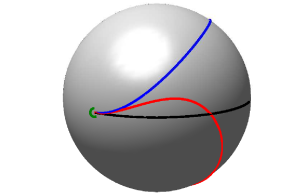
The Riemannian polynomial equation cannot, in general, be solved in closed form, and must be integrated numerically. In order to discretize this system of covariant differential equations, we implement the covariant integrator depicted in Alg. 1. At each step of the integrator, each vector is incremented within the tangent space at and the results are parallel transported infinitesimally along a geodesic from to . The only ingredients necessary to integrate a polynomial forward in time are the exponential map and parallel transport on the manifold.
Figure 1 shows the result of integrating polynomials of order one, two, and three. Initial velocity, acceleration, and jerk were chosen and a cubic polynomial integrated to obtain the blue curve. Then the initial jerk was set to zero and the blue quadratic curve was integrated, followed by the black geodesic whose acceleration was set to zero.
2.3 Estimation of Parameters for Regression
In order to regress polynomials against observed data , we define the following constrained objective function
| (11) | ||||
| (12) | ||||
| (13) | ||||
| (14) | ||||
| (15) | ||||
| (16) |
which is minimized in order to find the optimal initial conditions , which we will refer to as the parameters of our model.
In order to determine the optimal parameters , we introduce Lagrange multiplier vector fields , often called the adjoint variables, and define the unconstrained objective function
| (17) | ||||
| (18) | ||||
| (19) | ||||
| (20) |
As is standard practice, the optimality conditions for this equation are obtained by taking variations with respect to all arguments of , integrating by parts when necessary. The resulting variations with respect the the adjoint variables yield the original dynamic constraints: the polynomial equations. Variations with respect to the primal variables gives rise to the following system of equations, termed the adjoint equations. The adjoint equations take the following form (see appendix for derivation):
| (21) | ||||
| (22) | ||||
| (23) | ||||
| (24) |
where is the Riemannian curvature tensor and the Dirac functional indicates that the order zero adjoint variable takes on jump discontinuities at time points where data is present. Gradients of with respect to initial and final conditions give rise to the terminal endpoint conditions for the adjoint variables, as well as expressions for the gradients with respect to initial conditions.
| (25) | ||||
| (26) | ||||
| (27) |
In order to determine the value of the adjoint vector fields at , and thus the gradients of our functional , the adjoint variables are first initialized to zero at time , then the system Eq. 24 is evolved backward in time to .
Given the gradients with respect to the initial conditions, a simple steepest descent algorithm is used to optimize the functional. The update to is computed using the exponential map, and the vectors are updated via parallel translation.
Note that in the special case of a zero-order polynomial (), the only gradient is simply the mean of the log map vectors at the current estimate of the Fréchet mean. So this method generalizes the common method of Fréchet averaging on manifolds [Fletcher et al., 2004].
The curvature term, in the case , indicates that is a sum of adjoint Jacobi fields. So this approach subsumes geodesic regression as presented by Fletcher [Fletcher, 2011]. For higher order polynomials, the adjoint equations represent a generalized Jacobi system.
In practice, it is often not necessary to explicitly compute the curvature terms. In the case that the manifold embeds into a Hilbert space, the extrinsic adjoint equations can be computed by taking variations in the ambient space, using standard methods. Such an approach gives rise to the regression algorithm found in Niethammer et al. [Niethammer et al., 2011], for example.
2.4 Time Reparametrization
In the geodesic model, curves propagate at a constant speed, a result of their extremal action property. However, using higher-order polynomials it is possible to generate curves whose images match those of a geodesic, but whose time-dependence has been reparametrized. If the initial conditions consist of all collinear, then this will necessarily be the case. Polynomials provide flexibility not only in the class of paths that are possible, but in the time dependence of the curves traversing those paths. Regression models could even be imagined in which the operator wishes to estimate geodesic paths, but is unsure of parametrization, and so enforces the estimated parameters to be collinear.
2.5 Polynomials on Riemannian Lie Groups
A special case arises when the manifold is a Lie group and the metric is left-invariant. In this case, left-translation by and , denoted , allow one to isometrically represent tangent vectors at as tangent vectors at the identity, using the pushforward . The tangent space at the identity is isomorphically identified with the Lie algebra . The algebraic operation in is called the Lie bracket . For , this bracket operation, also called the adjoint action of on and often denoted , is bilinear and alternating in its arguments (i.e. ). Fixing , the operator is linear and its adjoint is computed with respect to the metric:
| (28) |
We will refer to the operator as the adjoint-transpose action of .
Suppose is a vector field along the curve and is its representative at the identity. Similarly, is the representative of the curve’s velocity in the Lie algebra. Then the covariant derivative of along evolves in the Lie algebra via
| (29) |
In the special case when so that , if we set this covariant derivative equal to zero we have the geodesic equation:
| (30) |
which in this form is often refered to as the Euler-Poincare equation [Arnol’d, 1989, Holm et al., 1998]. The curvature tensor is given by the standard formula
| (31) |
Applying Eq. 29, in a Lie group with left-invariant metric, these terms are computed in the Lie algebra using the formulas:
| (32) | ||||
| (33) | ||||
| (34) | ||||
| (35) |
Also note that if the metric is both left- and right-invariant, then the adjoint-transpose action is alternating and we can simplify the covariant derivative further. In particular, in the presence of such a bi-invariant metric, the first few covariant derivatives take the following forms:
| (36) | ||||
| (37) | ||||
| (38) | ||||
| (39) |
This allows us to solve the forward evolution in the convenient setting of the vector space . Parallel transport requires solution of the equation
| (40) |
which can be integrated using Euler integration or similar time-stepping algorithms, so long as the adjoint action can be easily computed. Because of the simplified covariant derivative formula for a bi-invariant metric, the curvature takes the simple form [do Carmo, 1992]:
| (41) |
2.6 Coefficient of Determination for Regression in Metric Spaces
It will be useful to define a statistic which will indicate how well our model fits some set of observed data. As in [Fletcher, 2011], we compute the coefficient of determination of our regression polynomial , denoted . The first step to computing is to compute the variance of the data. As discussed in [Fletcher, 2011], the natural choice of total variance statistic is the Fréchet variance, defined by
| (42) |
Note that the Fréchet mean itself is the 0-th order polynomial regression against the data and the variance is the value of the objective function at that point. We also define the sum of squared error for a curve as the value :
| (43) |
Then the coefficient of determination is defined as
| (44) |
Any regressed polynomial will have , will have a value between 0 and 1, with 1 indicating a perfect fit and 0 indicating that the curve provides no better fit than does the Fréchet mean.
3 Examples
3.1 The -Dimensional Sphere
Suppose . Then geodesics are great circles and the exponential map is given by
| (45) |
The corresponding log map is the inverse of this function:
| (46) |
The Riemannian curvature tensor is [do Carmo, 1992]
| (47) |
Parallel translation of a vector along the exponential map of a vector is performed as follows. The vector is decomposed into a vector parallel to , which we denote , and a vector orthogonal to , . is left unchanged by parallel transport along , while transforms in a similar way as :
| (48) |
Using this exponential map and parallel transport, the integrator depicted in Alg. 1 was implemented. Figure 1 shows the result of integrating polynomials of order one, two, and three, using the equations from this section, for the special case of a two-dimensional sphere.
3.2 The Lie Group
In order to illustrate the algorithm in a Lie group, we consider the Lie group of orthogonal 3-by-3 real matrices with determinant one. We review the basics of here, but the reader is encouraged to consult [Arnol’d, 1989] for a full treatment of and derivation of the Euler-Poincare equation there.
The Lie algebra for the rotation group is , the set of all skew-symmetric 3-by-3 real matrices. Such matrices can be identified with vectors in by the identification
| (55) |
under which the Lie bracket takes the convenient form of the cross-product of vectors:
| (56) |
With the representation of vectors in , an invariant metric is determined by the choice of a symmetric, positive-definite matrix :
| (57) |
With this metric the adjoint-transpose action can be written as
| (58) |
If we plug this into the general Lie group formula we obtain the geodesic equation in the Lie algebra:
| (59) |
which must be integrated numerically to find at each time. To compute the exponential map , the algorithm depicted in Alg. 1 is employed. The matrix is converted to a skew-symmetric matrix by multiplication by , which translates back into the Lie algebra. The resulting vector is converted to a vector . The geodesic equation is then integrated to find at future times. The point then evolves along the exponential map by time-stepping, where at each step is converted back into a skew-symmetric matrix , multiplied by and exponentiated to obtain a rotation matrix. The Euler step is then given by left-multiplication by the resulting matrix.
3.3 Kendall Shape Space
The analysis of shape is a common challenge in medical imaging. Shape is defined as the property of the data that is invariant to scale or rotation. It was in this setting that Kendall [Kendall, 1984] originally developed his theory of shape space. We describe here Kendall’s shape space of -landmark point sets in , denoted . For a more complete overview of Kendall’s shape space, including computation of the curvature tensor, the reader is encouraged to consult the work of Kendall and Le [Kendall, 1984, Kendall, 1989, Le and Kendall, 1993].
Let be a labelled pointset in . Translate the pointset so that the centroid resides at 0, removing any effects due to translations. Another degree of freedom due to scaling is removed by requiring that . After this standardization, one is left with a point in , commonly referred to as preshape space in this context.
Kendall shape space is obtained by taking the quotient of the preshape space by the natural action of the rotation group on pointsets. In practice, points in the quotient (refered to as shapes) are represented by a member of their equivalence class in preshape space. The work of O’Neill [O’Neill, 1966] characterizes the link in geometry between the shape and preshape spaces. We describe now how to compute exponential maps, log maps, and parallel transport in shape space, using representatives in .
First, notice that there exist tangent vectors in corresponding to global rotations of the preshape. At a particular point in preshape space, these vectors form a linear subspace of the tangent space , which we define as the vertical subspace. Curves moving along vertical tangent vectors result in rotations of a preshape, and so do not indicate any change in actual shape. Since we are concerned with shape change and wish to ignore effects due to rotation, it will be important to project such tangent vectors to be purely non-vertical, or horizontal. We denote the horizontal projection by .
A vertical vector in preshape space arises as the derivative of a rotation of a preshape. The derivative of such a rotation is a skew-symmetric matrix , and its action on a preshape has the form . The vertical subspace is then spanned by such tangent vectors arising from any linearly independent set of skew-symmetric matrices. The projection is performed by taking such a spanning set, performing Gram-Schmidt orthonormalization, and removing each component.
The horizontal projection allows us to relate the covariant derivative on the sphere to that on shape space. Lemma 1 of O’Neill [O’Neill, 1966] states that if are horizontal vector fields at some point in preshape space, then
| (65) |
where denotes the covariant derivative on preshape space and , and are their counterparts in shape space.
For a general shape space , the exponential map and parallel translation are performed using representatives in . In practice, this usually must be done in a time-stepping algorithm, in which at each time step an infinitesimal spherical parallel transport is performed, followed by the horizontal projection. The resulting algorithm can be used to compute the exponential map as well. Computation of the log map is less trivial, as it requires an iterative optimization routine. The target shape is first aligned to the base shape using Procrustes alignment. Then, at each iteration of the log map routine, the exponential map is integrated forward, compared to the target preshape, then the resulting tangent vector is adjoint parallel transported back to the base point, for update in a steepest descent iteration.
A special case arises in the case when . In this case the exponential map, parallel transport and log map have closed form. The reader is encouraged to consult [Fletcher, 2011] for more details about the two-dimensional case.
With exponential map, log map, and parallel transport implemented as described here, one can perform polynomial regression on Kendall shape space in any dimension. We demonstrate such regression now on examples in two dimensions.
3.3.1 Rat Calivarium Growth
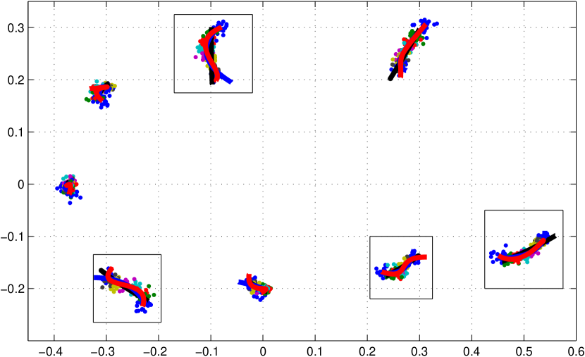
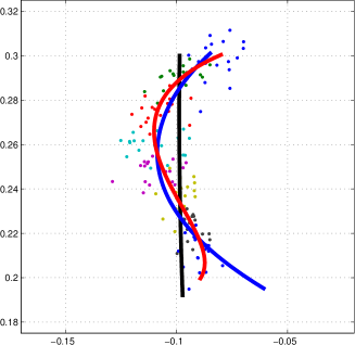
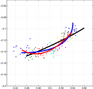
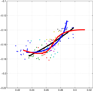
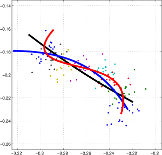
The first dataset we consider was first analyzed by Bookstein [Bookstein, 1991]. The data is available for download at http://life.bio.sunysb.edu/morph/data/datasets.html and consists of landmarks on a midsagittal section of rat calivaria (upper skulls). Landmark positions are available for 18 rats and at 8 ages apiece. Riemannian polynomials of orders were fit to this data. The resulting curves are shown in Fig. 2 and in zoomed detail in Fig. 3. Clearly the quadratic and cubic curves differ from that of the geodesic regression. The values agree with this qualitative difference: the geodesic regression has , while the quadratic and cubic regressions both have values of 0.85 and 0.87, respectively. While this shows that there is a clear improvement in the fit due to increasing from one to two, it also shows that little is gained by further increasing the order of the polynomial. Qualitatively, Fig. 3 shows that the slight increase in obtained by moving from a quadratic to cubic model corresponds to a marked difference in the curves, possibly indicating that the cubic curve is overfitting the data.
|
|
3.3.2 Corpus Callosum Aging
The corpus callosum is the major white matter bundle connecting the two hemispheres of the brain. In order to investigate shape change of the corpus callosum during normal aging, polynomial regression was performed on a collection of data from the OASIS brain database (www.oasis-brains.org). Magnetic resonance imaging (MRI) scans from 32 normal subjects with ages between 19 and 90 years were obtained from the database. A midsagittal slice was extracted from each volumetric image and segmented using the ITK-SNAP program (www.itksnap.org). Sets of 64 landmarks were optimized on the contours of these segmentations using the ShapeWorks program [Cates et al., 2007] (www.sci.utah.edu/software.html). The algorithm generates samplings of each shape boundary with optimal correspondences among the populaton.
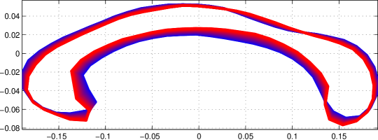
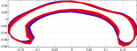
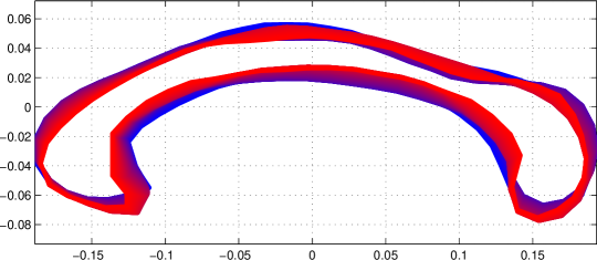
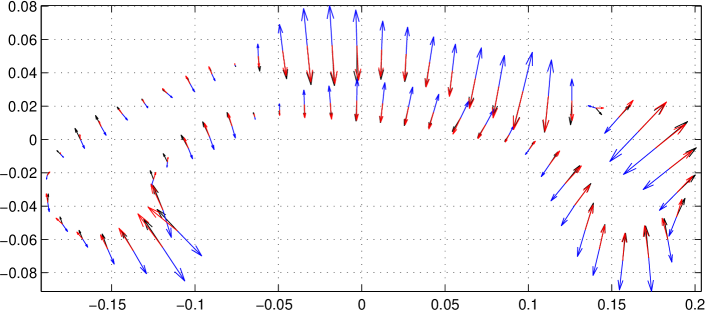
Regression results for geodesic, quadratic, and cubic regression are shown in Fig. 4. At first glance the results appear similar for the three different models, since the motion envelopes show close agreement. However, the values show an improvement from geodesic to quadratic (from 0.12 to 0.13) and from quadratic to cubic (from 0.13 to 0.21). Inspection of the estimated initial conditions, shown in Fig. 5 reveals that the tangent vectors appear to be rather collinear. For the reasons stated in Sec. 2.4, this suggests that the differences can essentially be described as reparametrization of the time variable, which is only accommodated in the higher order polynomial models.
Appendix: Derivation of Adjoint Equations
In this section we derive the adjoint system for the polynomial regression problem. The approach to calculus of variations followed here is outlined by, for example, Noakes et al. [Noakes et al., 1989]. Consider a simplified objective function containing only a single data term, at time :
| (66) |
Now consider taking variations of with respect to the vector fields . For each there are only two terms containing , so if is a test vector field along , then the variation of with respect to in the direction satisfies
| (67) |
The first term is integrated by parts to yield
| (68) |
The variation with respect to for is then given by
| (69) | ||||
| (70) | ||||
| (71) |
In order to determine the differential equation for , the variation with respect to must be computed. Let again denote a test vector field along . For some , let be a differentiable family of curves satisfying
| (72) | ||||
| (73) |
If is chosen small enough, the vector field can be extended to a neighborhood of such that , where a dot indicates the derivative in the direction. The vanishing Lie bracket implies the following identities
| (74) | ||||
| (75) |
Finally, the vector fields are extended along via parallel translation, so that
| (76) | ||||
| (77) |
The variation of with respect to satisfies
| (78) | ||||
| (79) | ||||
| (80) | ||||
| (81) |
As the are extended via parallel translation, their inner products satisfy
| (82) |
Then applying this to each term in the previous equation,
| (83) | ||||
| (84) | ||||
| (85) |
Then by construction, since ,
| (86) |
Then using the Lie bracket and curvature identities, this is written as
| (87) |
which is further simplified, again using the identity :
| (88) |
Using the Bianchi identities, it can be demonstrated that the curvature tensor satisfies the identity [do Carmo, 1992]:
| (89) |
for any vectors . The covariant derivative along is also integrated by parts to arrive at
| (90) |
Finally, gathering terms, the adjoint equation for and its gradients are obtained:
| (91) | ||||
| (92) | ||||
| (93) |
Along with the variations with respect to , this constitutes the full adjoint system. Extension to the case of multiple data at multiple time points is trivial, and results in the adjoint system presented in Sec. 2.3.
References
- [Arnol’d, 1989] Arnol’d, V. I. (1989). Mathematical Methods of Classical Mechanics. Springer, 2nd edition.
- [Bookstein, 1991] Bookstein, F. L. (1991). Morphometric Tools for Landmark Data: Geometry and Biology. Cambridge Univ. Press.
- [Cates et al., 2007] Cates, J., Fletcher, P. T., Styner, M., Shenton, M., and Whitaker, R. (2007). Shape modeling and analysis with entropy-based particle systems. In Proceedings of Information Processing in Medical Imaging (IPMI).
- [Davis et al., 2010] Davis, B. C., Fletcher, P. T., Bullitt, E., and Joshi, S. C. (2010). Population shape regression from random design data. International Journal of Computer Vision, 90(2):255–266.
- [do Carmo, 1992] do Carmo, M. P. (1992). Riemannian Geometry. Birkhäuser Boston, 1st edition.
- [Fletcher, 2011] Fletcher, P. T. (2011). Geodesic regression on Riemannian manifolds. In Proceedings of International Workshop on Mathematical Foundations of Computational Anatomy MFCA.
- [Fletcher et al., 2004] Fletcher, P. T., Liu, C., Pizer, S. M., and Joshi, S. C. (2004). Principal geodesic analysis for the study of nonlinear statistics of shape. IEEE Trans. Med. Imag., 23(8):995–1005.
- [Holm et al., 1998] Holm, D. D., Marsden, J. E., and Ratiu, T. S. (1998). The Euler-Poincaré equations and semidirect products with applications to continuum theories. Adv. in Math., 137:1–81.
- [Jupp and Kent, 1987] Jupp, P. E. and Kent, J. T. (1987). Fitting smooth paths to spherical data. Appl. Statist., 36(1):34–46.
- [Kendall, 1984] Kendall, D. G. (1984). Shape manifolds, Procrustean metrics, and complex projective spaces. Bull. London Math. Soc., 16(2):81–121.
- [Kendall, 1989] Kendall, D. G. (1989). A survey of the statistical theory of shape. Statistical Science, 4(2):87–99.
- [Kent et al., 2001] Kent, J. T., Mardia, K. V., Morris, R. J., and Aykroyd, R. G. (2001). Functional models of growth for landmark data. In Proceedings in Functional and Spatial Data Analysis, pages 109–115.
- [Le and Kendall, 1993] Le, H. and Kendall, D. G. (1993). The Riemannian structure of Euclidean shape spaces: A novel environment for statistics. Ann. Statist., 21(3):1225–1271.
- [Niethammer et al., 2011] Niethammer, M., Huang, Y., and Vialard, F.-X. (2011). Geodesic regression for image time-series. In Proceedings of Medical Image Computing and Computer Assisted Intervention (MICCAI).
- [Noakes et al., 1989] Noakes, L., Heinzinger, G., and Paden, B. (1989). Cubic splines on curved surfaces. IMA J. Math. Control Inform., 6:465–473.
- [O’Neill, 1966] O’Neill, B. (1966). The fundamental equations of a submersion. Michigan Math J., 13(4):459–469.