Sticky particle dynamics with interactions

Abstract.

We consider compressible pressureless fluid flows in Lagrangian coordinates in one space dimension. We assume that the fluid self-interacts through a force field generated by the fluid itself. We explain how this flow can be described by a differential inclusion on the space of transport maps, in particular when a sticky particle dynamics is assumed. We study a discrete particle approximation and we prove global existence and stability results for solutions of this system. In the particular case of the Euler-Poisson system in the attractive regime our approach yields an explicit representation formula for the solutions.

1. Introduction

In this paper, we consider a simple model for one-dimensional compressible fluid flows under the influence of a force field that is generated by the fluid itself. It takes the form of a hyperbolic conservation law for the density $\varrho$, which is a nonnegative measure in time and space and describes the distribution of mass or electric charge, and the real-valued Eulerian velocity field $v$. For suitable initial data $(\varrho,v)(t=0,\cdot)=:(\bar{\varrho},\bar{v})$, the unknowns $(\varrho,v)$ satisfy

$$\left.\begin{aligned} \partial_{t}\varrho+\partial_{x}(\varrho v)&=0\\ \partial_{t}(\varrho v)+\partial_{x}(\varrho v^{2})&=f[\varrho]\end{aligned}\right\}\quad\text{in $[0,\infty)\times\mathbb{R}$.}$$ (1.1)

The first equation in (1.1), called the continuity equation, describes the local conservation of mass or electric charge. Without loss of generality, we will assume in the following that the total mass/charge is equal to one initially and that the quadratic moment is finite so that $\varrho(t,\cdot)\in{\mathscr{P}}_{2}(\mathbb{R})$ for all $t\geqslant 0$, with ${\mathscr{P}}(\mathbb{R})$ the space of probability measures with finite quadratic moment. The second equation in (1.1) describes the conservation of momentum. We will assume in the following that $v(t,\cdot)\in{\mathscr{L}}^{2}(\mathbb{R},\varrho(t,\cdot))$ for all $t\geqslant 0$ so the kinetic energy is finite.

The continuous map $f\colon{\mathscr{P}}_{2}(\mathbb{R})\longrightarrow{\mathscr{M}}(\mathbb{R})$ in (1.1) describes the force field, with ${\mathscr{M}}(\mathbb{R})$ the space of all signed Borel measures with finite total variation. The force depends on the distribution of mass or electric charge and we will assume that $f[\varrho]$ is absolutely continuous with respect to $\varrho$. For further assumptions see Section 6. The typical (simplest) form of $f$ is

$$f[\varrho]=-\varrho\,\partial_{x}q_{\varrho}\quad\text{with}\quad q_{\varrho}(x)=V(x)+\int_{\mathbb{R}}W(x-y)\,{\mathrm{d}}\varrho(y)$$ (1.2)

for suitable ${\mathrm{C}}^{1}$ potential functions $V,W$ with (at most) linearly growing derivatives.

Another relevant example we have in mind is the Euler-Poisson system, for which

$$f[\varrho]=-\varrho\,\partial_{x}q_{\varrho}\quad\text{with $q_{\varrho}$ solution of}\quad-\partial_{xx}^{2}q_{\varrho}=\lambda(\varrho-\sigma).$$ (1.3)

When $\varrho$ is absolutely continuous with respect to the one-dimensional Lebesgue measure ${\mathcal{L}}^{1}$, then the function $q_{\varrho}$ admits a representation similar to (1.2), with

$$V(x):=-\frac{\lambda}{2}\int_{\mathbb{R}}|x-y|\,{\mathrm{d}}\sigma(y),\quad W(x):=\frac{\lambda}{2}|x|.$$ (1.4)

If $\rho$ is not absolutely continuous with respect to ${\mathcal{L}}^{1}$, then we have a similar representation with a nondifferentiable $W$, so that $f[\rho]$ must be defined by a suitable approximation process.

The Euler-Poisson equations in the repulsive regime (with $\lambda<0$ and negative concave potential $W$) is a simple model for semiconductors. In this case, $\varrho$ describes the electron or hole distribution and the scalar function $q_{\varrho}$ represents the electric potential generated by the distribution of charges in the material. Here $\sigma$ is the concentration of ionized impurities. The Euler-Poisson equations in the attractive regime (with $\lambda>0$ and positive convex potential $W$) is the one-dimensional version of a cosmological model for the universe at an early stage, describing the formation of galaxies. Now $q_{\varrho}$ represents the gravitational potential and $\sigma=0$.

1.1. Singular solutions and particle models.

Since there is no pressure in (1.1), there is no mechanism that forces the density $\varrho$ to be absolutely continuous with respect to the Lebesgue measure. In fact, the system (1.1) admits solutions that are singular measures. Assume that we are given initial data in the form of a finite linear combination of Dirac measures:

$$\bar{\varrho}=\sum_{i=1}^{N}\bar{m}_{i}\delta_{\bar{x}_{i}}\quad\text{and}\quad\bar{\varrho}\bar{v}=\sum_{i=1}^{N}\bar{m}_{i}\bar{v}_{i}\delta_{\bar{x}_{i}},$$ (1.5)

where $\bar{{\mbox{\boldmath$x$}}}=(\bar{x}_{1},\cdots,\bar{x}_{N})\in\mathbb{R}^{N}$ are the initial locations of $N$ particles denoted $P_{1},\cdots,P_{N}$, with corresponding masses $\bar{\mbox{\boldmath$m$}}=(\bar{m}_{1},\cdots,\bar{m}_{N})$ and initial velocities $\bar{\mbox{\boldmath$v$}}=(\bar{v}_{1},\cdots,\bar{v}_{N})$. We require that $\bar{m}_{i}>0$ and $\sum_{i}\bar{m}_{i}=1$ so that $\bar{\varrho}\in{\mathscr{P}}(\mathbb{R})$. For all times $t\geqslant 0$, we can assume that the positions ${\mbox{\boldmath$x$}}(t)=(x_{1}(t),\cdots,x_{N}(t))$ are monotonically ordered, so that they are unambiguously determined and attached to the particles. Then (at least formally) there is a solution of (1.1) in the form of a linear combination of Dirac measures:

$$\varrho(t,\cdot)=\sum_{i=1}^{N}m_{i}\delta_{x_{i}(t)}\quad\text{and}\quad(\varrho v)(t,\cdot)=\sum_{i=1}^{N}m_{i}v_{i}(t)\delta_{x_{i}(t)},$$ (1.6)

where the functions $(x_{i},v_{i})$ solve the system of ordinary differential equations

$$\dot{x}_{i}(t)=v_{i}(t),\quad\dot{v}_{i}(t)=a_{\bar{\mbox{\scriptsize\boldmath$m$}},i}({\mbox{\boldmath$x$}}(t))\quad\text{and}\quad(x_{i},v_{i})(t=0)=(\bar{x}_{i},\bar{v}_{i})$$ (1.7)

between particle collisions. Here $a_{{\mbox{\scriptsize\boldmath$m$}},i}({\mbox{\boldmath$x$}})\color[rgb]{0,0,0}$ is the value in the point $x_{i}(t)$ of the Radon-Nikodym derivative of the force $f[\varrho]$ with respect to the measure $\varrho$, so that

$$f[\varrho]=\sum_{i=1}^{N}a_{{\mbox{\scriptsize\boldmath$m$}},i}({\mbox{\boldmath$x$}})\,m_{i}\delta_{x_{i}}\quad\text{if}\quad\varrho=\sum_{i=1}^{N}m_{i}\,\delta_{x_{i}},$$ (1.8)

which is well defined when all $N$ particles are distinct.

Upon collision of, say, two particles with masses $m_{k}$ and $m_{k+1}$ at some time $t>0$, the velocities of each one of them are changed to

$$v_{k}(t+)=v_{k+1}(t+)=\frac{m_{k}v_{k}(t-)+m_{k+1}v_{k+1}(t-)}{m_{k}+m_{k+1}},$$ (1.9)

so that the momentum is preserved during the collision. Since both particles continue their journey with the same velocity, they may be considered as one bigger particle with mass $m_{k}+m_{k+1}$. Collisions of more than two particles can be handled in a similar fashion. We will refer to any solution of (1.1) in the form (1.6) as a discrete particle solution and we will say that it satisfies a global sticky condition if particles after collision are not allowed to split. In this case, after each collision, one could relabel the particles so that the system (1.7) still makes sense (with $N$ reduced in each particle collision) and induces a global in time evolution.

Let us denote by $\mathbb{K}^{N}$ the closed cone

$$\mathbb{K}^{N}:=\big{\{}{\mbox{\boldmath$x$}}\in\mathbb{R}^{N}:x_{1}\leqslant x_{2}\leqslant\cdots\leqslant x_{N}\big{\}},$$ (1.10)

whose interior is $\mathop{\rm int}\nolimits{\mathbb{K}^{N}}=\big{\{}{\mbox{\boldmath$x$}}\in\mathbb{R}^{N}:x_{1}<x_{2}<\cdots<x_{N}\big{\}}$. The construction of discrete particle solutions as outlined above can be done rigorously whenever the functions $a_{{\mbox{\scriptsize\boldmath$m$}},i}:\mathop{\rm int}\nolimits{\mathbb{K}^{N}}\to\mathbb{R}^{N}$ are uniformly continuous in each bounded set (so that they admit a continuous extension to $\mathbb{K}^{N}$ still denoted by $a_{{\mbox{\scriptsize\boldmath$m$}},i}$) and satisfies the compatibility condition

$$a_{{\mbox{\scriptsize\boldmath$m$}},k}({\mbox{\boldmath$x$}})=a_{{\mbox{\scriptsize\boldmath$m$}},k+1}({\mbox{\boldmath$x$}})\quad\text{if $x_{k}=x_{k+1}$ for some $1\leqslant k<N$.}$$ (1.11)

This is certainly the case when the potentials $V,W$ considered in (1.2) are of class ${\mathrm{C}}^{1}$. On the other hand, the case of the Euler-Poisson system is much more subtle and presents different features in the attractive or the repulsive case.

The Euler-Poisson case in the repulsive regime: splitting and collapsing of masses

Let us consider the simplest situation of $N$ distinct particles with equal initial velocities $\bar{v}$, in the repulsive regime $\lambda=-1$ with $\sigma=0$. Let $M_{0}:=0$, $M_{i}:=\sum_{j=1}^{i}m_{j}$ for $i=1,\ldots,N$ and set $A_{i}:=\frac{1}{2}(M_{i-1}+M_{i}-1)$. Then it is not difficult to check (see Example 6.9) that in the repulsive regime

$$a_{{\mbox{\scriptsize\boldmath$m$}},i}({\mbox{\boldmath$x$}})=A_{i}\quad\text{for all $i$ if ${\mbox{\boldmath$x$}}\in\mathop{\rm int}\nolimits{\mathbb{K}^{N}}$,}$$ (1.12)

and so there is no continuous extension satisfying (1.11). Starting from distinct initial positions, particles follow (at least for a small time interval) the free motion paths

$$x_{i}(t)=\bar{x}_{i}+t\bar{v}+\frac{1}{2}A_{i}t^{2}.$$ (1.13)

Since $A_{i}\leqslant A_{i+1}$ for all $i$, there are no collisions. Taking the limit as the initial positions of two or more particles coincide we obtain the same representation for every ${\mbox{\boldmath$x$}}\in\mathbb{K}^{N}$. On the other hand, if two particles $P_{k},P_{k+1}$ coincide at the time $t=0$, i.e. $\bar{x}_{k}=\bar{x}_{k+1}=\bar{x}$ with the same initial velocity $\bar{v}$, then the “sticky” solution $x_{k}(t)=x_{k+1}(t)=\bar{x}+t\bar{v}+\frac{1}{4}(A_{k}+A_{k+1})t^{2}$ gives raise to an admissible solution to (1.1) which is different from the previous one. One could also consider a solution where $P_{k},P_{k+1}$ stick in a small initial time interval $[0,s]$ and then evolve according to (1.13).

Considering a situation where the number $N$ of admissible particles grows to infinity with a uniform initial mass distribution concentrating at the origin, one can guess that a “repulsive” solution arising from a unit mass concentrated at $\bar{x}$ should istantaneously diffuse, becoming absolutely continuous with respect to the Lebesgue measure ${\mathcal{L}}^{1}$: the explicit formula is

$$\varrho(t,\cdot)=u(t,\cdot){\mathcal{L}}^{1}\quad\text{with}\quad u(t,x)=\frac{1}{2t^{2}}{\raise 1.29167pt\hbox{$\chi$}}_{(\bar{x}+\bar{v}t-\frac{1}{4}t^{2},\bar{x}+\bar{v}t+\frac{1}{4}t^{2})}(x)\quad\text{for all $x\in\mathbb{R}$ and $t\geqslant 0$.}$$ (1.14)

An even more complicated situation occurs e.g. if $\bar{v}_{i}=0$ for $i\neq k,k+1$, but $\bar{v}_{k}>0>\bar{v}_{k+1}$ in such a way that a collision occurs between $P_{k}$ and $P_{k+1}$ at some time $t=r$, after which the particles could stick or wait for some time and then evolve as in the previous example.

It would be important to find a selection mechanism that gives raise to a stable notion of solution and to obtain a continuous model by passing to the limit in the number of particles. In this paper we study a criterium of the following type : Assume that two particle $P_{k},P_{k+1}$ collide at some time $r>0$ with incoming velocities $v_{k}(r_{-})\geqslant v_{k+1}(r_{-})$. Then the particles will stick together for all times $r<t<s$ provided that $s$ is small enough so that

$$v_{k}(r_{-})+\int_{r}^{t}a_{{\mbox{\scriptsize\boldmath$m$}},k}({\mbox{\boldmath$x$}}(\tau))\,{\mathrm{d}}\tau\geqslant v_{k}(t)=v_{k+1}(t)\geqslant v_{k+1}(r_{-})+\int_{r}^{t}a_{{\mbox{\scriptsize\boldmath$m$}},k+1}({\mbox{\boldmath$x$}}(\tau))\,{\mathrm{d}}\tau$$ (1.15)

for all $r<t<s$. Conversely, if (1.15) becomes false for some time $s>r$, then the particles may separate again. A rigorous formulation of condition (1.15) in the case of a simultaneous collision or separation of more than two particles, or of a continuous distribution of masses, can be better understood in the famework of differential inclusions in a Lagrangian setting, which we will describe in Section 5.1. Before giving an idea of this approach, let us brefly consider how (1.15) greatly simplifies in the attractive regime.

The attractive Euler-Poisson system and the sticky condition

In the attractive case, we can simply invert the signs in (1.12). It turns out, however, that the behaviour of the two-particles example considered in the previous paragraph changes completely, since the limit when two particles collapse exhibit a strong stability: after a collision, two or more particles stick together and do not split ever again, giving raise to a global sticky solution.

This reflects the fact that the sticky condition in the attractive regime implies (1.15) for all $s>r$: the functions $a_{{\mbox{\scriptsize\boldmath$m$}},i}$ defined by the negative of (1.12) always satisfy $a_{{\mbox{\scriptsize\boldmath$m$}},k}({\mbox{\boldmath$x$}})\geqslant a_{{\mbox{\scriptsize\boldmath$m$}},k+1}({\mbox{\boldmath$x$}})$ and the incoming velocities of two particles $P_{k},P_{k+1}$ colliding at some time $r$ satisfies $v_{k}(r-)\geqslant v_{k+1}(r_{-})$, so that any sticky evolution corresponding to $x_{k}(t)=x_{k+1}(t)$ for $t\geqslant r$ will satisfy (1.15).

As we shall see, the differential description in the Lagrangian setting we will adopt encodes (1.15) and corresponds to a sticky condition whenever the acceleration field is continuous (as in (1.11)) or it is of attractive type. In the repulsive case it will model a suitable relaxation mechanism allowing for separation of particles after collision, still preserving the stability of the evolution.

1.2. Lagrangian description and differential inclusions

In this paper, we will give an interpretation of system (1.1) in the framework of differential inclusions. As before, let us first consider the simpler case of the dynamic of a finite number of particles. We can identify the positions of a collection of particles $P_{1},\cdots,P_{N}$ with a vector ${\mbox{\boldmath$x$}}=(x_{1},\cdots,x_{N})\in\mathbb{R}^{N}$: since we labeled the particles in a monotone way, it is not admissible for particles to pass by one another, so the order of the locations must be preserved and the vector $x$ is confined in the closed convex cone $\mathbb{K}^{N}$ defined by (1.10). Denoting by ${\mbox{\boldmath$v$}}=(v_{1},\cdots,v_{N})\in\mathbb{R}^{N}$ the vector of the velocities of the particles, their trajectories between collisions are mostly determined by a system of differential equation

$$\dot{\mbox{\boldmath$x$}}(t)={\mbox{\boldmath$v$}}(t),\quad\dot{\mbox{\boldmath$v$}}(t)={\mbox{\boldmath$a$}}_{\mbox{\scriptsize\boldmath$m$}}({\mbox{\boldmath$x$}}(t)),$$ (1.16)

where ${\mbox{\boldmath$a$}}_{\mbox{\scriptsize\boldmath$m$}}({\mbox{\boldmath$x$}}):=(a_{{\mbox{\scriptsize\boldmath$m$}},1}({\mbox{\boldmath$x$}}),\cdots,a_{{\mbox{\scriptsize\boldmath$m$}},N}({\mbox{\boldmath$x$}}))$ is a vector field defined for ${\mbox{\boldmath$x$}}\in\mathbb{K}^{N}$ as in (1.7), which in the simplest case is continuous. Whenever the vector ${\mbox{\boldmath$x$}}(t)$ hits the boundary of the domain

$$\partial\mathbb{K}^{N}:=\big{\{}{\mbox{\boldmath$x$}}\in\mathbb{K}^{N}:\Omega_{\mbox{\scriptsize\boldmath$x$}}\neq\varnothing\big{\}},\quad\Omega_{\mbox{\scriptsize\boldmath$x$}}:=\big{\{}j\colon x_{j}=x_{j+1},j=1\ldots N-1\big{\}},$$ (1.17)

however, an instantaneous force changes its velocity in such a way that it stays inside of $\mathbb{K}^{N}$.

In order to find a mathematical model that describes this situation, we must first identify the set of admissible velocities at each point ${\mbox{\boldmath$x$}}\in\mathbb{K}^{N}$, which is called the tangent cone of $\mathbb{K}^{N}$ at $x$. It is defined by

$$T_{\mbox{\scriptsize\boldmath$x$}}\mathbb{K}^{N}:=\mathrm{cl}\Big{\{}\theta({\mbox{\boldmath$y$}}-{\mbox{\boldmath$x$}}):{\mbox{\boldmath$y$}}\in\mathbb{K}^{N},\ \theta\geqslant 0\Big{\}}.$$ (1.18)

In our situation, it is not difficult to check that

$$T_{\mbox{\scriptsize\boldmath$x$}}\mathbb{K}^{N}=\Big{\{}{\mbox{\boldmath$v$}}\in\mathbb{R}^{N}\colon\text{$v_{j}\leqslant v_{j+1}$ for all $j\in\Omega_{\mbox{\scriptsize\boldmath$x$}}$}\Big{\}}.$$ (1.19)

Identity (1.19) shows that when two particles collide, then the velocity of the left particle cannot be greater than the velocity of the right particle, so the left particle cannot pass.

Assume now that ${\mbox{\boldmath$x$}}(t)\in\partial\mathbb{K}^{N}$ at some time $t$ and let ${\mbox{\boldmath$v$}}(t-)$ be the velocity immediately before the impact. That is, let ${\mbox{\boldmath$v$}}(t-)$ be the left-derivative of the curve $t\mapsto{\mbox{\boldmath$x$}}(t)$ at time $t$. The instantaneous force that is active on impact must change the velocity to a new value in the tangent cone $T_{{\mbox{\scriptsize\boldmath$x$}}(t)}\mathbb{K}^{N}$ of admissible velocities. Typically, there are many possibilities. Assuming inelastic collisions, we impose the impact law:

$${\mbox{\boldmath$v$}}(t+):=\mathsf{P}_{\raisebox{3.01389pt}{\scriptsize{$T_{{\mbox{\boldmath$\scriptscriptstyle x$}}(t)}\mathbb{K}^{N}$}}}{\mbox{\boldmath$v$}}(t-),$$ (1.20)

where ${\mbox{\boldmath$v$}}(t+)$ is the velocity immediately after impact (the right-derivative of ${\mbox{\boldmath$x$}}(t)$). We denote by ${\sf P}\kern-1.0pt_{T_{{\mbox{\boldmath$\scriptscriptstyle x$}}(t)}\mathbb{K}^{N}}$ the metric projection onto $T_{{\mbox{\scriptsize\boldmath$x$}}(t)}\mathbb{K}^{N}$ so that

$$\|{\mbox{\boldmath$v$}}(t-)-{\mbox{\boldmath$v$}}(t+)\|=\min\Big{\{}\|{\mbox{\boldmath$v$}}(t-)-{\mbox{\boldmath$u$}}\|_{\mbox{\scriptsize\boldmath$m$}}\colon{\mbox{\boldmath$u$}}\in T_{{\mbox{\scriptsize\boldmath$x$}}(t)}\mathbb{K}^{N}\Big{\}}.$$

Hence ${\mbox{\boldmath$v$}}(t+)$ is the element in $T_{{\mbox{\scriptsize\boldmath$x$}}(t)}\mathbb{K}^{N}$ closest to ${\mbox{\boldmath$v$}}(t-)$ with respect to the weighted Euclidean distance induced by the norm

$$\|{\mbox{\boldmath$v$}}\|_{{\mbox{\scriptsize\boldmath$m$}}}:=\sqrt{\sum_{i=1}^{N}m_{i}v^{2}_{i}}\quad\text{for all ${\mbox{\boldmath$v$}}\in T_{{\mbox{\scriptsize\boldmath$x$}}(t)}\mathbb{K}^{N}\subset\mathbb{R}^{N}$,}$$ (1.21)

and therefore unique: see Figure 1 for a graphic representation of this rule.

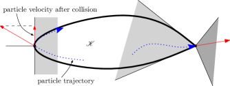
Figure 1. Projection of velocities onto the tangent cone.

It is well-known that the metric projection onto closed convex cones admits a variational characterization of its minimizers; see [Zarantonello]. In particular, we have

$$\Big{(}{\mbox{\boldmath$v$}}(t-)-{\mbox{\boldmath$v$}}(t+)\Big{)}\cdot{\mbox{\boldmath$u$}}\leqslant 0\quad\text{for all ${\mbox{\boldmath$u$}}\in T_{{\mbox{\scriptsize\boldmath$x$}}(t)}\mathbb{K}^{N}$.}$$

We deduce that the instantaneous force that changes the velocity upon impact onto the boundary $\partial\mathbb{K}^{N}$, must be an element of the normal cone $N_{{\mbox{\scriptsize\boldmath$x$}}(t)}\mathbb{K}^{N}$, which is defined as

$$N_{\mbox{\scriptsize\boldmath$x$}}\mathbb{K}^{N}:=\Big{\{}{\mbox{\boldmath$n$}}\in\mathbb{R}^{N}\colon\text{${\mbox{\boldmath$n$}}\cdot({\mbox{\boldmath$y$}}-{\mbox{\boldmath$x$}})\leqslant 0$ for all ${\mbox{\boldmath$y$}}\in\mathbb{K}^{N}$}\Big{\}}.$$ (1.22)

Note that the normal cone $N_{\mbox{\scriptsize\boldmath$x$}}\mathbb{K}^{N}$ equals the subdifferential $\partial I_{\mathbb{K}^{N}}({\mbox{\boldmath$x$}})$ of the indicator function $I_{\mathbb{K}^{N}}$ of $\mathbb{K}^{N}$ at the point $x$. This follows immediately from the definition of the subdifferential.

This suggests to consider the second-order differential inclusion

$$\dot{{\mbox{\boldmath$x$}}}={\mbox{\boldmath$v$}},\quad\dot{{\mbox{\boldmath$v$}}}+N_{{\mbox{\scriptsize\boldmath$x$}}}\mathbb{K}^{N}\ni{\mbox{\boldmath$a$}}_{\mbox{\scriptsize\boldmath$m$}}({\mbox{\boldmath$x$}})\quad\text{in $[0,\infty)$.}$$ (1.23)

Notice that since $v$ can exhibit jumps, solutions to (1.23) should be properly defined in a weak sense in the framework of functions of bounded variation. Second-order differential inclusion have been studied in the literature and existence of solutions has been shown in a genuinely finite dimensional setting. We refer the reader to [BernicotVernel, Moreau, Schatzman] and the references therein for further information. Due to the possible nonuniqueness of solutions to second-order differential inclusions [Schatzman] and to the lack of estimates to pass to the limit when $N\to\infty$, we need a better understanding of the particular features of our setting, in particular of the convex cones $\mathbb{K}^{N}$.

The sticky condition and an equivalent formulation of (1.23)

It has been shown in [NatileSavare] that the one-parameter family of normal cones $N_{{\mbox{\scriptsize\boldmath$x$}}(t)}\mathbb{K}^{N}$ along an evolution curve ${\mbox{\boldmath$x$}}:[0,\infty)\to\mathbb{K}^{N}$ for which a gobal stickyness condition holds, satisfies the remarkable monotonicity property

$$N_{{\mbox{\scriptsize\boldmath$x$}}(s)}\mathbb{K}^{N}\subset N_{{\mbox{\scriptsize\boldmath$x$}}(t)}\mathbb{K}^{N}\quad\text{for all $s<t$.}$$ (1.24)

Consequently, for any selection ${\mbox{\boldmath$\xi$}}:[0,\infty)\to\mathbb{R}^{N}$ satisfying ${\mbox{\boldmath$\xi$}}(t)\in N_{{\mbox{\scriptsize\boldmath$x$}}(t)}\mathbb{K}^{N}$ (such as ${\mbox{\boldmath$a$}}_{\mbox{\scriptsize\boldmath$m$}}({\mbox{\boldmath$x$}}(t))-\dot{\mbox{\boldmath$v$}}(t)$ in (1.23)) we have

$$\int_{s}^{t}{\mbox{\boldmath$\xi$}}(r)\,{\mathrm{d}}r\in N_{{\mbox{\scriptsize\boldmath$x$}}(t)}\mathbb{K}^{N}\quad\text{for all $s<t$.}$$

An integration of (1.23) yields, at least formally, that

$${\mbox{\boldmath$v$}}(t)+N_{{\mbox{\scriptsize\boldmath$x$}}(t)}\mathbb{K}^{N}\ni{\mbox{\boldmath$v$}}(s)+\int_{s}^{t}{\mbox{\boldmath$a$}}({\mbox{\boldmath$x$}}(r))\,{\mathrm{d}}r$$

and therefore the system (1.23) can be rewritten in the form

$$\dot{\mbox{\boldmath$x$}}={\mbox{\boldmath$v$}},\quad{\mbox{\boldmath$v$}}+N_{{\mbox{\scriptsize\boldmath$x$}}}\mathbb{K}^{N}\ni{\mbox{\boldmath$y$}},\quad\dot{\mbox{\boldmath$y$}}={\mbox{\boldmath$a$}}_{\mbox{\scriptsize\boldmath$m$}}({\mbox{\boldmath$x$}}).$$ (1.25)

Introducing new unknowns $({\mbox{\boldmath$x$}},{\mbox{\boldmath$y$}})$, we can rewrite (1.25) as a first order evolution inclusion

$$\dot{\mbox{\boldmath$x$}}+N_{{\mbox{\scriptsize\boldmath$x$}}(t)}\mathbb{K}^{N} \ni{\mbox{\boldmath$y$}}$$ (1.26)

$$\dot{\mbox{\boldmath$y$}} ={\mbox{\boldmath$a$}}_{\mbox{\scriptsize\boldmath$m$}}({\mbox{\boldmath$x$}})$$

for which an existence and stability theory is available, at least when ${\mbox{\boldmath$a$}}_{\mbox{\scriptsize\boldmath$m$}}$ is a Lipschitz map.

We will show that formulation (1.26) enjoys interesting features and always induces a measure-valued solution to (1.1). When the field ${\mbox{\boldmath$a$}}_{\mbox{\scriptsize\boldmath$m$}}$ satisfies the compatibility condition (1.11), solutions to (1.26) satisfies the sticky condition, and the same property holds also for the Euler-Poisson equation in the attractive regime. In the repulsive case, we will see that (1.26) is a robust formulation of condition (1.15). Let us now consider the infinite-dimensional case.

1.3. Diffuse measures and differential inclusions for Lagrangian parametrizations

In order to deal with general measure-valued solutions of (1.1), we had to recourse to Lagrangian coordinates, using ideas of optimal transport as considered in [NatileSavare].

Monotone Lagrangian rearrangemens

In this approach, the discrete set of parameters $\{1,2,\cdots,N\}$ involved in the representation of discrete particle measures (1.5) will be substituted by $\Omega=(0,1)$. For every particle labeled by $m\in\Omega$, we will denote by $X(t,m)\in\mathbb{R}$ its position at time $t$. The map $X$ can be uniquely characterized in terms of the measure $\varrho$: it is the uniquely determined nondecreasing and right-continuous map $X:\Omega\to\mathbb{R}$ such that

$$X(m)\leqslant x\quad\Longleftrightarrow\quad m\leqslant\varrho\big{(}(-\infty,x]\big{)}\quad\text{for all $x\in\mathbb{R}$}.$$ (1.27)

Equivalently, the push-forward $X_{\#}\mathfrak{m}$ of the one-dimensional Lebesgue measure $\mathfrak{m}:={\mathcal{L}}^{1}|_{\Omega}$ under the map $X$ equals $\varrho$. Recall that the push-forward measure is defined by

$$X_{\#}\mathfrak{m}(A):=\mathfrak{m}(X^{-1}(A))\quad\text{for all Borel sets $A\subset\mathbb{R}$.}$$ (1.28)

Therefore the map $X$ is the optimal transport map pushing $\mathfrak{m}$ forward to $\varrho$. We refer the reader to Section 2 for further explanation.

In this way, to any solution $(\varrho,v)$ of (1.1), we can associate a map $X\colon[0,\infty)\times\Omega\longrightarrow\mathbb{R}$ with $X(t,\cdot)$ nondecreasing and a velocity $V:[0,+\infty)\times\Omega\to\mathbb{R}$ such that

$$X(t,\cdot)_{\#}\mathfrak{m}=\varrho(t,\cdot)\quad\text{for all $t\geqslant 0$},\quad V(t,\cdot)=v(t,X(t,\cdot))=\partial_{t}X(t,\cdot).$$ (1.29)

Our goal is to show that (1.1) can be associated to a differential inclusion in terms of $(X,V)$. This observation allows us to derive existence and stability results (see Sections 3 and 4) for (suitably defined) solutions of (1.1), which together with the existence of discrete particle solutions (see Section 5) imply a global existence result for (1.1) for general initial data; see Section 6.

Differential inclusions

The framework of first-order differential inclusions, analogous to the setting we already discussed for the discrete case (1.23), serves as a guiding principle for our discussion. The role of the cone $\mathbb{K}^{N}$ is now played by the cone of optimal transport maps

$${\mathscr{K}}:=\Big{\{}X\in{\mathscr{L}}^{2}(\Omega)\colon\text{$X$ is nondecreasing}\Big{\}}$$ (1.30)

in the Hilbert space ${\mathscr{H}}:={\mathscr{L}}^{2}(\Omega)$. Even if in this infinite dimensional setting the boundary of ${\mathscr{K}}$ is dense, we can still consider the normal cone $N_{X}{\mathscr{K}}$ for given $X\in{\mathscr{K}}$, which is given by

$$N_{X}{\mathscr{K}}:=\Big{\{}W\in{\mathscr{L}}^{2}(\Omega)\colon\text{$\int_{\Omega}W\Big{(}\tilde{X}-X\Big{)}\,{\mathrm{d}}m\leqslant 0$ for all $\tilde{X}\in{\mathscr{K}}$}\Big{\}}.$$ (1.31)

Again we have that $N_{X}{\mathscr{K}}=\partial I_{\mathscr{K}}(X)$. It can be shown that $N_{X}{\mathscr{K}}=\{0\}$ if and only if the map $X$ is not strictly increasing in $\Omega$. That is, whenever $\Omega_{X}\neq\varnothing$ where

$$\Omega_{X}:=\Big{\{}m\in\Omega\colon\text{$X$ is constant in a neighborhood of $m$}\Big{\}}.$$ (1.32)

Note that $\Omega_{X}$ is the complement of the support of the distributional derivative of $X$.

Consider now a family of densities $t\mapsto\varrho(t,\cdot)$ that satisfies (1.1). Let $t\mapsto X(t,\cdot)\in{\mathscr{K}}$ be the associated family of optimal transport maps; see (1.29). We want to interpret $X$ as a solution of differential inclusions, similar to (1.23) and (1.26).

Even at the continuous level, the monotonicity property (1.24) for sticky particle evolutions plays a crucial role. Note that the optimal transport map $X\in{\mathscr{K}}$ takes a constant value $x\in\mathbb{R}$ on some interval $(\alpha,\beta)\subset\Omega$ if the mass $\beta-\alpha$ (the Lebesgue measure of the interval) is moving to the same location, thereby forming a Dirac measure at $x$. Therefore sticky evolutions will be characterized as curves $t\mapsto X(t,\cdot)$ with the property that

for any $$t_{1}\leqslant t_{2} \Omega_{X(t_{1})}\subset\Omega_{X(t_{2})}$$ we have . (1.33)

Notice that (1.33) implies that once a Dirac measure is formed, it may accrete more mass over time, but it can never lose mass. It also implies the following statement: It is not possible for mass to jump from one side of a Dirac measure to the opposite side. Whenever mass is crossing a Dirac measure, it gets absorbed.

A formulation via differential inclusions needs a Lagrangian expression of the force term in (1.1). That is, we must find a map $F\colon{\mathscr{K}}\longrightarrow{\mathscr{L}}^{2}(\Omega)$ with the property that

$$\int_{\mathbb{R}}\psi(x)\,f[\varrho](dx)=\int_{\Omega}\psi(X(m))F[X](m)\,{\mathrm{d}}m\quad\text{for all $\psi\in{\mathscr{D}}(\mathbb{R})$,}$$ (1.34)

whenever $X\in{\mathscr{K}}$ and $X_{\#}\mathfrak{m}=\varrho$. We refer the reader to Section 6 for further discussion about the existence and properties of maps $F$ satisfying (1.34). In the following, we will assume that $F$ is continuous as a map of ${\mathscr{K}}$ into ${\mathscr{L}}^{2}(\Omega).$

We then could expect $X$ to be a solution of a second-order differential inclusion, but arguing as for the discrete case (1.23) at least in the case of sticky evolutions (1.33) we end up with

$$\dot{X}(t)+\partial I_{\mathscr{K}}(X(t))\ni\bar{V}+\int_{0}^{t}F[X(s)]\,{\mathrm{d}}s$$ (1.35)

for a.e. $t>0$. This formulation and its consequences is at the heart of our argument.

It is a remarkable fact (see Theorem 3.5) that solutions to (1.35) always parametrize measure-valued solutions to the partial differential equation (1.1). Provided $F$ satisfies suitable continuity properties, it will be possible to prove existence (and uniqueness, when $F$ is Lipschitz) of solutions to (1.35) for any initial data $(\bar{X},\bar{V})\in{\mathscr{K}}\times{\mathscr{L}}^{2}(\Omega)$ by combining the theory of gradient flows of convex functionals in Hilbert spaces [Brezis] with suitable compactness arguments.

When $F$ satisfies a suitable sticking condition, which is satisfied e.g. in the case of ${\mathrm{C}}^{1}$ potentials in (1.2) and of the Euler-Poisson system in the attractive regime, then solutions to (1.35) form a semigroup and have the sticky evolution property (1.33). Even for general $F$ (and in particular for the Euler-Poisson system in the repulsive regime) the differential inclusion (1.35) still selects a stable parametrization of solutions to (1.1). This is somewhat surprising since the reduction from second-order to first-order differential inclusion was motivated by the monotonicity (1.33), which typically is false without additional assumptions on $F$. In this Introduction we refer to such solutions as “robust.”

Representation formulae for the Euler-Poisson system

In the case of the Euler-Poisson system (1.3) with $\sigma=0$ one can show that the Lagrangian representation of the force $f$ is given by

$$F[X](m)=-\lambda A(m)\quad\text{where}\quad A(m):=m-\frac{1}{2}.$$ (1.36)

Note that the map $F[X]$ is independent of $X$ and (1.35) becomes

$$\dot{X}(t)+\partial I_{\mathscr{K}}(X(t))\ni\bar{V}-\lambda tA$$

In the attractive regime when $\lambda\geq 0$, an explicit representation formula for the Lagrangian solution can be obtained (see Theorems 6.11). In fact a careful analysis shows that the solution $X$ to (1.35) can be computed by solving the trivial ODE in $X$ obtained by eliminating the ${\mathscr{K}}$-constraint:

$$\frac{{\mathrm{d}}}{{\mathrm{d}}t}\tilde{X}(t)=\bar{V}-\lambda tA$$

(whose solution is $\tilde{X}(t)=\bar{X}+t\,\bar{V}-\frac{1}{2}\lambda t^{2}A$), and then projecting $\tilde{X}$ on ${\mathscr{K}}$:

$$X(t)={\sf P}\kern-1.0pt_{{\mathscr{K}}}(\tilde{X}(t))={\sf P}\kern-1.0pt_{{\mathscr{K}}}\bigg{(}\bar{X}+t\,\bar{V}-\frac{1}{2}\lambda t^{2}A\bigg{)}.$$

Applying the characterization given in [NatileSavare], the metric projection of ${\sf P}\kern-1.0pt_{{\mathscr{K}}}$ onto ${\mathscr{K}}$ can be found by introducing the primitive functions

$$\bar{\mathcal{X}}(m):=\int_{0}^{m}\bar{X}(\ell)\,{\mathrm{d}}\ell,\quad\bar{\mathcal{V}}(m):=\int_{0}^{m}\bar{V}(\ell)\,{\mathrm{d}}\ell,\quad\mathcal{A}(m):=\frac{1}{2}(m^{2}-m),$$

and the time evolution

$$\mathcal{X}(t,m):=\bar{\mathcal{X}}(m)+t\,\bar{\mathcal{V}}(m)-\frac{1}{2}\lambda t^{2}\mathcal{A}(m),$$

and then taking the derivative with respect to $m$ of the convex envelope $\mathcal{X}^{**}(t,\cdot)$ of $\mathcal{X}(t,\cdot)$:

$$X(t,m)=\frac{\partial}{\partial m}\mathcal{X}^{**}(t,m),$$

which defines a density $\varrho_{t}=X(t)_{\#}\mathfrak{m}$. It is then a simple exercise to recover formula (1.14) in the case $\bar{X}(m)\equiv\bar{x},\ \bar{V}(m)\equiv\bar{v}$, since $\mathcal{X}(t,m)=\mathcal{X}^{**}(t,m)$ and $X(t,m)=\bar{x}+t\bar{v}+\frac{1}{2}t^{2}(m-\frac{1}{2}).$

1.4. Time discrete schemes

In this section, we show that the first-order differential inclusion (1.35) can be used to design a stable explicit numerical scheme to compute robust solutions to (1.1). In fact, this scheme is essentially the same as the one introduced in [Brenier2] for “order-preserving vibrating strings” and “sticky particles”, with just mild modifications. For simplicity, we concentrate on the pressureless repulsive Euler-Poisson system with a neutralizing background

$$\partial_{t}\varrho+\partial_{x}(\varrho v) =0,$$ (1.37)

$$\partial_{t}(\varrho v)+\partial_{x}(\varrho v^{2}) =-\varrho\,\partial_{x}q_{\varrho}\qquad-\partial_{xx}q_{\varrho}=-(\varrho-1),$$ (1.38)

(cf. (1.3) with $\lambda=-1$ and $\sigma=1$). We assume the initial conditions to be 1-periodic in $x$ and the density $\varrho$ to have unit mean so that the system is globally neutral and the electric potential $q_{\varrho}$ is 1-periodic in $x$. Note that we choose the periodic setting only for convenience. In fact, for any non-periodic solution $\varrho$ of (1.1), one could consider the push-forward of $\varrho$ under the map $x\mapsto x-[x]$ for all $x\in\mathbb{R}$, with $[x]$ the largest integer not greater than $x$. One obtains a new density $\varrho^{*}$ that is concentrated on $[0,1)$ and therefore can be extended 1-periodically to the whole real line. One can then show that $\varrho^{*}$ satisfies the same equation. We refer the reader to [GangboTudorascu] for details.

For smooth solutions without mass concentration, written in mass coordinates

$$V(t,m)=\dot{X}(t,m)=v(t,X(t,m)),\quad\partial_{m}X(t,m)\varrho(t,X(t,m))=1$$

(which requires that $\partial_{m}X(t,m)\geqslant 0$), one can show that the whole system reduces to a collection of independent linear pendulums labeled by their equilibrium position $m$ and subject to

$$\dot{X}(t,m)=V(t,m),\quad\dot{V}(t,m)+X(t,m)-m=0.$$ (1.39)

(Notice that, due to the spatial periodicity of the initial conditions, the new unknown $X(t,m)-m$ and $V(t,m)$ are 1-periodic in $m$.) This reduction is valid as long as the pendulums stay “well-ordered” and do not cross each other, i.e., as long as $X(t,m)$ stays monotonically nondecreasing in $m$. This “non-crossing” condition is not sustainable for large initial conditions and collision generally occur in finite time. To handle sticky collisions, the concept of robust solutions introduced in Section 1.3 is a good way to obtain a well-posed mathematical model beyond collisions.

We are now ready to describe the semi-discrete scheme. Given a time step $\tau>0$ and suitable initial data $(\bar{X},\bar{V})=:(X_{\tau,0},V_{\tau,0})$, we denote by $(X_{\tau,n}(m),V_{\color[rgb]{0,0,0}\tau,n}(m))$ the approximate solution at time $t_{n}:=n\tau$, for $n=0,1,2,\ldots$, defined in two steps as follows:

1. Predictor step: we first integrate the ODE (1.39) and get $U_{\tau,n+1}$ and $\hat{X}_{\tau,n+1}$ accordingly

   $$\hat{X}_{\tau,n+1}(m)=m+(X_{\tau,n}(m)-m)\cos(\tau)+V_{\tau,n}(m)\sin(\tau),$$ (1.40)

   $$V_{\tau,n+1}(m)=-(X_{\tau,n}(m)-m)\sin(\tau)+V_{\tau,n}(m)\cos(\tau).$$ (1.41)

2. Corrector step: we rearrange $\hat{X}_{\tau,n+1}(m)$ in nondecreasing order with respect to $m$ and obtain $X_{\tau,n+1}(m)$. Because of the periodic boundary conditions, we have to perform this step with care. We rely on the existence, for each map $m\mapsto Y(m)$ such that $Y(m)-m$ is 1-periodic and locally Lebesgue integrable, of a unique map $m\mapsto Y^{*}(m)$ such that $Y^{*}(m)$ is nondecreasing in $m$ and

   $$\int_{0}^{1}\eta(Y^{*}(m))\,{\mathrm{d}}m=\int_{0}^{1}\eta(Y(m))\,{\mathrm{d}}m$$

   for all continuous 1-periodic function $\eta$.

This time discrete scheme becomes a fully discrete scheme, if the initial data $X_{\tau,0}(m)-m$ and $V_{\tau,0}(m)$ are piecewise constant on a uniform cartesian grid with step $h$. (We just have to be careful with the corrector step, by using a suitable sorting algorithm for periodic data.)

To illustrate the scheme, we show the numerical solutions corresponding to initial conditions

$$X_{0}(m)=m,\quad V_{0}(m)=4\sin(2\pi m).$$ (1.42)

We use 400 equally spaced grid points $m$ (which corresonds to 400 “well-ordered” pendulums with $m$ as equilibrium position) and $5000$ time steps (see Figures 2–4):

Figure 2. Space-time trajectories of pendulums, with timestep $\tau=0.001$.

Figure 3. Space-time trajectories of pendulums, with timestep $\tau=0.005$.

Figure 4. Space-time trajectories of pendulums, with timestep $\tau=0.01$.

$$\tau=0.001,\quad 0.005,\quad 0.01,$$

so that the final time $T$ of observation is respectively given by

$$T=5,\quad 25,\quad 50.$$

On each picture, we show the space-time trajectories of 50 of the 400 pendulums, with space coordinate on the horizontal axis and time coordinate on the vertical one. On these pictures, we observe a strong concentration, with sticky collisions, of the pendulums at a very early stage (up to time $t=\pi/2$) around $x=0.5$. Later on, some pendulums start to unstick and detach from each other (which allows new concentrations at later times $t\geqslant\pi$ around $x=0$ and $x=1$). Much later, after $t=10\pi$, there is no further dissipation of energy, and, as pendulums touch each other, they always do so with zero relative speed. Then the corrector step is no longer active, and the scheme becomes exact (due to the exact integration of the predictor step). At this late stage, the solution becomes $2\pi$-periodic in time. We study the convergence of the scheme in Section 7.

1.5. Plan of the paper

We collect in Section 2 a few basic results on optimal transport in one dimension, on convex analysis (concerning in particular the properties of the convex cone ${\mathscr{K}}$), and on convex functionals in ${\mathscr{L}}^{2}(\Omega)$.

In Section 3, after a brief discussion of the basic properties of the Lagrangian force functional $F$, we introduce the notion of Lagrangian solutions to the differential inclusion (1.35). Theorem 3.5 collects their main properties, in particular in connection with measure-valued solutions to (1.1). Sections 3.3 and 3.5 provide the main existence, uniqueness, and stability results for Lagrangian solutions, whereas Section 3.4 is devoted to the particular case of sticky evolutions.

We study in Section 4 a different class of solutions to (1.35), still linked to (1.1), that naturally arise as limit of sticky particle systems when $F$ does not obey the sticking condition. These solutions exhibit better semigroup properties than the Lagrangian solutions introduced in Section 3, but lack uniqueness.

Section 5 we carefully study the dynamics of discrete particle systems, which we already briefly discussed in the Introduction. Discrete Lagrangian solutions associated to systems like (1.26) are treated in Section 5.1, where we also show that they can be used to approximate any continuous Lagrangian solution, as the one considered in Section 3. The sticky dynamic at the particle level is considered in §5.2: the main Theorem 5.2 provides the basic results, which allow us to replace second-order with first-order evolution inclusion at the discrete level and to get sticky evolutions for sticking forces. The particle approach is a crucial step of our analysis, since it avoids many technical difficulties arising at the continuous level. The general idea is to prove fine properties of the solutions (such as the monotonicity (1.33) in the sticking case or a representation formula) at the discrete level and then to extend them to the general case by applying suitable stability results with respect to the initial conditions. Those are typically obtained by applying contraction estimates (in the case when $F$ is Lipschitz) or compactness via Helly’s Theorem, by exploiting higher integrability and monotonicity of transport maps.

Section 6 applies the Lagrangian formulation to (1.1), presenting some existence and stability results for solutions in the Eulerian formalism.

In Section 7 we prove the convergence of the time discrete scheme introduced in Section 1.4.

2. Preliminaries

Let us first gather some definitions and results that will be needed later.

2.1. Optimal Transport

We denote by ${\mathscr{P}}(\mathbb{R}^{m})$ the space of all Borel probability measures on $\mathbb{R}^{m}$. The push-forward $\nu:=Y_{\#}\mu$ of a given measure $\mu\in{\mathscr{P}}(\mathbb{R}^{m})$ under a Borel map $Y\colon\mathbb{R}^{m}\longrightarrow\mathbb{R}^{n}$ is the measure defined by $\nu(A):=\mu(Y^{-1}(A))$ for all Borel sets $A\subset\mathbb{R}^{n}$. We will repeatedly use the change-of-variable formula

$$\int_{\mathbb{R}^{n}}\zeta(y)\,(Y_{\#}\mu)({\mathrm{d}}y)=\int_{\mathbb{R}^{m}}\zeta(Y(x))\,\mu({\mathrm{d}}x),$$ (2.1)

which holds for all Borel maps $\zeta\colon\mathbb{R}^{n}\longrightarrow[0,\infty]$.

We denote by ${\mathscr{P}}_{2}(\mathbb{R}^{n})$ the space of all Borel probability measures $\varrho\in{\mathscr{P}}(\mathbb{R}^{n})$ with finite quadratic moment: $\int_{\mathbb{R}^{n}}|x|^{2}\,\varrho({\mathrm{d}}x)<\infty$. The ${\mathscr{L}}^{2}$ Kantorovich-Rubinstein-Wasserstein distance $W_{2}(\varrho_{1},\varrho_{2})$ between two measures $\varrho_{1},\varrho_{2}\in{\mathscr{P}}_{2}(\mathbb{R}^{n})$ can be defined in terms of couplings, i.e. of probability measures ${\boldsymbol{\varrho}}\in{\mathscr{P}}(\mathbb{R}^{n}\times\mathbb{R}^{n})$ satisfying $\pi^{i}_{\#}{\boldsymbol{\varrho}}=\varrho_{i}$ for $i=1\ldots 2$, by the formula

$$W_{2}^{2}(\varrho_{1},\varrho_{2}):=\min\bigg{\{}\int_{\mathbb{R}^{n}\times\mathbb{R}^{n}}|x-y|^{2}\,{\boldsymbol{\varrho}}({\mathrm{d}}x,{\mathrm{d}}y)\colon{\boldsymbol{\varrho}}\in{\mathscr{P}}(\mathbb{R}^{n}\times\mathbb{R}^{n}),\pi^{i}_{\#}{\boldsymbol{\varrho}}=\varrho_{i}\bigg{\}}.$$ (2.2)

Here $\pi^{i}(x_{1},x_{2}):=x_{i}$ is the projection on the $i$th coordinate. It can be shown that there always exists an optimal transport plan ${\boldsymbol{\varrho}}$ for which the $\inf$ in (2.2) is in fact attained. We denote by $\Gamma_{\mathrm{opt}}(\varrho_{1},\varrho_{2})$ the set of optimal transport plans.

In the one-dimensional case $n=1$, there exists a unique coupling ${\boldsymbol{\varrho}}\in\Gamma_{\mathrm{opt}}(\varrho_{1},\varrho_{2})$ realizing the minimum of (2.2) (at least when the cost is finite). It can be explicitly characterized by inverting the distribution functions of $\varrho_{1}$ and $\varrho_{2}$: for any $\varrho\in{\mathscr{P}}(\mathbb{R})$ we consider its cumulative distribution function, which is defined as

$$M_{\varrho}(x):=\varrho\big{(}(-\infty,x]\big{)}\quad\text{for all $x\in\mathbb{R}$.}$$ (2.3)

Note that then $\varrho=\partial_{x}M_{\varrho}$ in ${\mathscr{D}}^{\prime}(\mathbb{R})$. Its monotone rearrangement is given by

$$X_{\varrho}(m):=\inf\Big{\{}x\colon M_{\varrho}(x)>m\Big{\}}\quad\text{for all $m\in\Omega$,}$$ (2.4)

where $\Omega:=(0,1)$. The map $X_{\varrho}$ is right-continuous and nondecreasing. We have

$$\mathfrak{m}:={\mathcal{L}}^{1}\lower 3.0pt\hbox{$|_{\Omega}$},\quad(X_{\varrho})_{\#}\mathfrak{m}=\varrho\quad\text{and}\quad\int_{\mathbb{R}}\zeta(x)\,\varrho({\mathrm{d}}x)=\int_{\Omega}\zeta(X_{\varrho}(m))\,{\mathrm{d}}m$$ (2.5)

for all Borel maps $\zeta\colon\mathbb{R}\longrightarrow[0,\infty]$. In particular, we have that $\varrho\in{\mathscr{P}}_{2}(\mathbb{R})$ if and only if $X_{\varrho}\in{\mathscr{L}}^{2}(\Omega)$. The Hoeffding-Fréchet theorem [Rachev-Ruschendorf98I]*Section 3.1 shows that the joint map $X_{\varrho_{1},\varrho_{2}}\colon\Omega\longrightarrow\mathbb{R}\times\mathbb{R}$ defined by

$$X_{\varrho_{1},\varrho_{2}}(m):=\Big{(}X_{\varrho_{1}}(m),X_{\varrho_{2}}(m)\Big{)}\quad\text{for all $m\in\Omega$,}$$

characterizes the optimal coupling ${\boldsymbol{\varrho}}\in\Gamma_{\mathrm{opt}}(\varrho_{1},\varrho_{2})$ by the formula

$${\boldsymbol{\varrho}}=(X_{\varrho_{1},\varrho_{2}}\big{)}_{\#}\mathfrak{m};$$ (2.6)

see [DallAglio56, Rachev-Ruschendorf98I, Villani] for further information. As a consequence, we obtain that

$$W_{2}^{2}(\varrho_{1},\varrho_{2})=\int_{\Omega}|X_{\varrho_{1}}(m)-X_{\varrho_{2}}(m)|^{2}\,{\mathrm{d}}m=\|X_{\varrho_{1}}-X_{\varrho_{2}}\|^{2}_{{\mathscr{L}}^{2}(\Omega)}.$$ (2.7)

The map $\varrho\mapsto X_{\varrho}$ is an isometry between ${\mathscr{P}}_{2}(\mathbb{R})$ and ${\mathscr{K}}$, where ${\mathscr{K}}\subset{\mathscr{L}}^{2}(\Omega)$ is the set of nondecreasing functions. Without loss of generality, we may consider precise representatives of nondecreasing functions only, which are defined everywhere.

2.2. Some Tools of Convex Analysis for ${\mathscr{K}}$

Let ${\mathscr{K}}$ be the collection of right-continuous nondecreasing functions in ${\mathscr{L}}^{2}(\Omega)$ introduced in (1.30). Then one can check that ${\mathscr{K}}$ is a closed convex cone in the Hilbert space ${\mathscr{L}}^{2}(\Omega)$.

Metric Projection and Indicator Function

It is well-known that the metric projection onto a nonempty closed convex set of an Hilbert space is a well defined Lipstchitz map (see e.g. [Zarantonello]): we denote it by ${\sf P}\kern-1.0pt_{{\mathscr{K}}}\colon{\mathscr{L}}^{2}(\Omega)\longrightarrow{\mathscr{K}}$. For all ${X}\in{\mathscr{L}}^{2}(\Omega)$ it is characterized by

$$Y={\sf P}\kern-1.0pt_{{\mathscr{K}}}({X})\quad\Longleftrightarrow\quad Y\in{\mathscr{K}},\quad\|Y-X\|_{{\mathscr{L}}^{2}(\Omega)}\leqslant\|\tilde{Y}-{X}\|_{{\mathscr{L}}^{2}(\Omega)}\quad\text{for every }\tilde{Y}\in{\mathscr{K}},$$

or, equivalently, by the following families of variational inequalities

$$Y={\sf P}\kern-1.0pt_{{\mathscr{K}}}({X})\quad\Longleftrightarrow\quad Y\in{\mathscr{K}},\quad\int_{\Omega}({X}-Y)(\tilde{Y}-Y)\leqslant 0\quad\text{for all $\tilde{Y}\in{\mathscr{K}}$.}$$ (2.8)

${\sf P}\kern-1.0pt_{{\mathscr{K}}}(X)$ admits a more explicit characterization in terms of the convex envelope of the primitive of $X$ [NatileSavare, Theorem 3.1]:

$$Y={\sf P}\kern-1.0pt_{{\mathscr{K}}}(X)=\frac{{\mathrm{d}}^{+}}{{\mathrm{d}}m}\mathcal{X}^{**}(m),\quad\mathcal{X}(m):=\int_{0}^{m}X(\ell)\,{\mathrm{d}}\ell,$$ (2.9)

where $\frac{{\mathrm{d}}^{+}}{{\mathrm{d}}m}$ denotes the right derivative and

$$\mathcal{X}^{**}(m):=\sup\Big{\{}a+b\,m\colon a,b\in\mathbb{R},\quad a+b\,m\leqslant\mathcal{X}(m)\quad\forall\,m\in(0,1)\Big{\}}$$ (2.10)

is the greatest convex and l.s.c. function below $\mathcal{X}$.

Let now $I_{\mathscr{K}}\colon{\mathscr{L}}^{2}(\Omega)\longrightarrow[0,+\infty]$ be the indicator function of ${\mathscr{K}}$, defined as

$$I_{\mathscr{K}}(X):=\begin{cases}0&\text{if $X\in{\mathscr{K}}$,}\\ +\infty&\text{otherwise,}\end{cases}$$

which is convex and lower semicontinuous. Its subdifferential is given by

$$\partial I_{\mathscr{K}}(X):=\bigg{\{}Z\in{\mathscr{L}}^{2}(\Omega)\colon\text{$I_{\mathscr{K}}(X)\geqslant I_{\mathscr{K}}(X)+\int_{\Omega}Z(X-X)$ for all $X\in{\mathscr{L}}^{2}(\Omega)$}\Big{\}}$$ (2.11)

and it is a maximal monotone operator in ${\mathscr{L}}^{2}(\Omega)$; in particular its graph is strongly-weakly closed in ${\mathscr{L}}^{2}(\Omega)\times{\mathscr{L}}^{2}(\Omega)$. Notice that $\partial I_{\mathscr{K}}(X)=\varnothing$ for all $X\not\in{\mathscr{K}}$ since in this case $I_{\mathscr{K}}(X)=\infty$; whenever $X\in{\mathscr{K}}$ we find that

$$\partial I_{\mathscr{K}}(X)=\bigg{\{}Z\in{\mathscr{L}}^{2}(\Omega)\colon\text{$0\geqslant\int_{\Omega}Z(X-X)$ for all $X\in{\mathscr{K}}$}\Big{\}},$$ (2.12)

so that $\partial I_{\mathscr{K}}(X)$ coincides with the normal cone $N_{X}{\mathscr{K}}$ defined by (1.31).

(2.8) implies the following equivalence: For all $X,Y\in{\mathscr{L}}^{2}(\Omega)$ we have

$$Y={\sf P}\kern-1.0pt_{{\mathscr{K}}}(X)\quad\Longleftrightarrow\quad X-Y\in\partial I_{\mathscr{K}}(Y).$$ (2.13)

Decomposing $X=Y+Z$ in (2.13) with $Y,Z\in{\mathscr{L}}^{2}(\Omega)$, we find that

$$Z\in\partial I_{\mathscr{K}}(Y)\quad\Longleftrightarrow\quad Y={\sf P}\kern-1.0pt_{{\mathscr{K}}}(Y+Z).$$ (2.14)

Lemma 2.1 (Contraction).

Let $\psi\colon\mathbb{R}\longrightarrow(-\infty,+\infty]$ be a convex, lower semicontinuous function. For all $X_{1},X_{2}\in{\mathscr{L}}^{2}(\Omega)$ we then have

$$\int_{\Omega}\psi({\sf P}\kern-1.0pt_{{\mathscr{K}}}(X_{1})-{\sf P}\kern-1.0pt_{{\mathscr{K}}}(X_{2}))\leqslant\int_{\Omega}\psi(X_{1}-X_{2}).$$

In particular, the metric projection ${\sf P}\kern-1.0pt_{{\mathscr{K}}}$ is a contraction with respect to the ${\mathscr{L}}^{p}(\Omega)$-norm with $p\in[1,\infty]$ and for all $X_{1},X_{2}\in{\mathscr{L}}^{2}(\Omega)$ we can estimate

$$\|{\sf P}\kern-1.0pt_{{\mathscr{K}}}(X_{1})-{\sf P}\kern-1.0pt_{{\mathscr{K}}}(X_{2})\|_{{\mathscr{L}}^{p}(\Omega)}\leqslant\|X_{1}-X_{2}\|_{{\mathscr{L}}^{p}(\Omega)}.$$ (2.15)

We refer the reader to Theorem 3.1 in [NatileSavare] for a proof. Notice that by choosing $X_{2}=0$ in Lemma 2.1, for which ${\sf P}\kern-1.0pt_{{\mathscr{K}}}(X_{2})=0$, we obtain the inequalities

$$\int_{\Omega}\psi({\sf P}\kern-1.0pt_{{\mathscr{K}}}(X))\leqslant\int_{\Omega}\psi(X)\quad\text{for all $X\in{\mathscr{L}}^{2}(\Omega)$,}$$ (2.16)

$$\vphantom{\int}\|{\sf P}\kern-1.0pt_{{\mathscr{K}}}(X)\|_{{\mathscr{L}}^{p}(\Omega)}\leqslant\|X\|_{{\mathscr{L}}^{p}(\Omega)}\quad\text{for all $X\in{\mathscr{L}}^{2}(\Omega)$.}$$ (2.17)

A similar result holds for the ${\mathscr{L}}^{2}$-orthogonal projection ${\sf P}\kern-1.0pt_{{\mathscr{H}}_{X}}$ onto the closed subspace ${\mathscr{H}}_{X}$, $X\in{\mathscr{K}}$, defined by

$${\mathscr{H}}_{X}:=\Big{\{}U\in{\mathscr{L}}^{2}(\Omega)\colon\text{$U$ is constant in each interval $(\alpha,\beta)\subset\Omega_{X}$}\Big{\}}.$$ (2.18)

Notice that we have ${\sf P}\kern-1.0pt_{{\mathscr{H}}_{X}}(V)=V$ a.e. in $\Omega\setminus\Omega_{X}$ and

$${\sf P}\kern-1.0pt_{{\mathscr{H}}_{X}}(V)=\fint_{\alpha}^{\beta}V(s)\,{\mathrm{d}}s\quad\text{in any maximal interval $(\alpha,\beta)\subset\Omega_{X}$,}$$ (2.19)

for all $V\in{\mathscr{L}}^{2}(\Omega)$. Jensen’s inequality then easily yields

Lemma 2.2 (${\mathscr{H}}_{X}$–Contraction).

Let $\psi:\mathbb{R}\to[0,\infty]$ be a convex l.s.c. function. Then for all $X\in{\mathscr{K}}$ we have

$$\int_{\Omega}\psi({\sf P}\kern-1.0pt_{{\mathscr{H}}_{X}}(X))\,{\mathrm{d}}m\leqslant\int_{\Omega}\psi(X)\,{\mathrm{d}}m.$$

For any pair of functions $X,Y\in{\mathscr{L}}^{1}(\Omega)$ we say that $Y$ is dominated by $X$ and we write $Y\prec X$ if the value of each convex integral functional on $Y$ is less than the corresponding value on $X$, i.e.

$$Y\prec X\quad\Leftrightarrow\quad\int_{\Omega}\psi(Y)\,{\mathrm{d}}m\leqslant\int_{\Omega}\psi(X)\,{\mathrm{d}}m$$

for all convex, lower semicontinuous $\psi\colon\mathbb{R}\longrightarrow[0,\infty]$. Estimate (2.16) shows that ${\sf P}\kern-1.0pt_{{\mathscr{K}}}(X)\prec X$ for all $X\in{\mathscr{L}}^{2}(\Omega)$.

Normal and Tangent Cones

It is immediate to check that the subdifferential (2.11) of the indicator function $I_{\mathscr{K}}$ coincides with the normal cone $N_{X}{\mathscr{K}}$ of ${\mathscr{K}}$ at $X\in{\mathscr{K}}$ defined by (1.31). Applying [NatileSavare, Thm. 3.9] we get the following useful characterization:

Lemma 2.3.

Let $X\in{\mathscr{K}}$ be given. For given $W\in{\mathscr{L}}^{2}(\Omega)$ we denote by

$$\Xi_{W}(m):=\int_{0}^{m}W(s)\,{\mathrm{d}}s\quad\text{for all $m\in[0,1]$,}$$

its primitive. Then $W\in N_{X}{\mathscr{K}}$ if and only if $\Xi_{W}\in{\mathcal{N}}_{X}$, where

$${\mathcal{N}}_{X}:=\Big{\{}\Xi\in{\mathrm{C}}([0,1])\colon\text{$\Xi\geqslant 0$ in $[0,1]$ and $\Xi=0$ in $\Omega\setminus\Omega_{X}$}\Big{\}}.$$

That is, a function $W$ is in the normal cone $N_{X}{\mathscr{K}}$ if and only if it is the derivative of a nonnegative function $\Xi$ that vanishes in $\Omega\setminus\Omega_{X}$. This implies in particular that $W$ vanishes a.e. in $\Omega\setminus\Omega_{X}$. Moreover, for any maximal interval $(\alpha,\beta)$ in the open set $\Omega_{X}$ we have that $\Xi(\alpha)=\Xi(\beta)=0$, by continuity of $\Xi$. Thus

$$\int_{\alpha}^{\beta}W(s)\,{\mathrm{d}}s=0\quad\text{for any maximal interval $(\alpha,\beta)\subset\Omega_{X}$.}$$ (2.20)

For later use, we also highlight the following fact: Let $X_{1},X_{2}\in{\mathscr{K}}$. Then

$$\Omega_{X_{1}}\subset\Omega_{X_{2}}\quad\Longrightarrow\quad N_{X_{1}}{\mathscr{K}}\subset N_{X_{2}}{\mathscr{K}}.$$ (2.21)

This follows immediately from the corresponding monotonicity for ${\mathcal{N}}_{X}$.

Let us now consider the Tangent cone $T_{X}{\mathscr{K}}$ to ${\mathscr{K}}$ at $X\in{\mathscr{K}}$: it can be defined as in (1.18) by

$$T_{X}{\mathscr{K}}:=\mathrm{cl}\Big{(}\bigcup_{\theta\geq 0}\theta({\mathscr{K}}-X)\Big{)}=\mathrm{cl}\Big{\{}\theta(\tilde{X}-X):\tilde{X}\in{\mathscr{K}},\ \theta\geq 0\Big{\}},$$ (2.22)

or, equivalently, as the polar cone of $N_{X}{\mathscr{K}}$, i.e.

$$T_{X}{\mathscr{K}}:=\Big{\{}U\in{\mathscr{L}}^{2}(\Omega)\colon\text{$\int_{\Omega}U(m)W(m)\,{\mathrm{d}}m\leqslant 0$ for all $W\in N_{X}{\mathscr{K}}$}\Big{\}}.$$ (2.23)

Lemma 2.4.

Let $X\in{\mathscr{K}}$ be given. Then

$$T_{X}{\mathscr{K}}=\Big{\{}U\in{\mathscr{L}}^{2}(\Omega)\colon\text{$U$ is nondecreasing in each interval $(\alpha,\beta)\subset\Omega_{X}$}\Big{\}}.$$

More precisely, the map $U\in T_{X}{\mathscr{K}}$ must be nondecreasing up to Lebesgue null sets. We may assume that $U$ is right-continuous in each $(\alpha,\beta)\subset\Omega_{X}$.

Proof of Lemma 2.4.

Let $U\in T_{X}{\mathscr{K}}$ be given and fix some interval $(\alpha,\beta)\subset\Omega_{X}$. For all nonnegative $\varphi\in{\mathscr{D}}(\Omega)$ with $\operatorname{{\mathrm{spt}}}\varphi\subset(\alpha,\beta)$ we have $\varphi^{\prime}\in N_{X}{\mathscr{K}}$ because of Lemma 2.3. By definition of the tangent cone $T_{X}{\mathscr{K}}$ we find that

$$\int_{\alpha}^{\beta}U(m)\varphi^{\prime}(m)\,{\mathrm{d}}m\leqslant 0\quad\text{for all nonnegative $\varphi\in{\mathscr{D}}(\Omega)$ with $\operatorname{{\mathrm{spt}}}\varphi\subset(\alpha,\beta)$.}$$

This shows that the distributional derivative of $U$ in $(\alpha,\beta)$ is a nonnegative Radon measure, and so $U$ is nondecreasing in the interval.

Conversely, assume that $U\in{\mathscr{L}}^{2}(\Omega)$ is nondecreasing in each interval $(\alpha,\beta)$ that is contained in $\Omega_{X}$. For any $W\in N_{X}{\mathscr{K}}$ we then decompose the integral

$$\int_{\Omega}U(m)W(m)\,{\mathrm{d}}m=\int_{\Omega\setminus\Omega_{X}}U(m)W(m)\,{\mathrm{d}}m+\sum_{n}\int_{\alpha_{n}}^{\beta_{n}}U(m)W(m)\,{\mathrm{d}}m,$$ (2.24)

where the sum is over all maximal intervals $(\alpha_{n},\beta_{n})\subset\Omega_{X}$ (at most countably many). Then the first integral on the right-hand side vanishes because $W(m)=0$ for a.e. $m\in\Omega\setminus\Omega_{X}$. For each integral in the sum, an approximation argument (see again Lemma 3.10 in [NatileSavare]) allows us to integrate by parts to obtain

$$\int_{\alpha_{n}}^{\beta_{n}}U(m)W(m)\,{\mathrm{d}}m=-\int_{\alpha_{n}}^{\beta_{n}}\Xi_{W}(s)\gamma(ds),$$

where $\gamma$ is the distributional derivative of $U$ in $(\alpha_{n},\beta_{n})$. Since $U$ is assumed nondecreasing and $\Xi_{W}$ is nonnegative, we conclude that $U\in T_{X}{\mathscr{K}}$. ∎

Recalling Lemma 2.4 it is immediate to check that

$$U\in{\mathscr{H}}_{X}\quad\Longleftrightarrow\quad U\text{ and }-U\ \in T_{X}{\mathscr{K}}.$$ (2.25)

Observe that if $X_{1},X_{2}\in{\mathscr{K}}$ then

$$\Omega_{X_{1}}\subset\Omega_{X_{2}}\quad\Longrightarrow\quad{\mathscr{H}}_{X_{2}}\subset{\mathscr{H}}_{X_{1}}.$$ (2.26)

Whenever $U\in{\mathscr{H}}_{X}$, then (2.24) equals zero because every term in the sum vanishes since $U$ is constant and $W$ has vanishing average. Thus

$$N_{X}{\mathscr{K}}\subset{\mathscr{H}}_{X}^{\perp}\quad\text{for all $X\in{\mathscr{K}}$,}$$ (2.27)

with ${\mathscr{H}}_{X}^{\perp}$ the orthogonal complement of ${\mathscr{H}}_{X}$. In particular

$$Y={\sf P}\kern-1.0pt_{{\mathscr{K}}}(X)\quad\Longrightarrow\quad Y={\sf P}\kern-1.0pt_{{\mathscr{H}}_{Y}}(X),\quad{\mathscr{H}}_{Y}\subset{\mathscr{H}}_{X}.$$ (2.28)

We have in fact a more precise characterization of ${\mathscr{H}}^{\perp}_{X}$ in terms of $N_{X}{\mathscr{K}}$: in the following, let us denote by $\mathscr{I}(\Omega_{X})$ the collection of all maximal intervals $(\alpha,\beta)$ (the connected components) of $\Omega_{X}$.

Lemma 2.5.

For every $X\in{\mathscr{K}}$ the closed subspace ${\mathscr{H}}^{\perp}_{X}$ is

$${\mathscr{H}}^{\perp}_{X}=\Big{\{}W\in{\mathscr{L}}^{2}(\Omega) :W=0\ \text{a.e.\ in }\Omega\setminus\Omega_{X},$$ (2.29)

$$\int_{\alpha}^{\beta}W(m)\,{\mathrm{d}}m=0\quad\text{for every }(\alpha,\beta)\in\mathscr{I}(\Omega_{X})\Big{\}},$$

and it is the closed linear subspace of ${\mathscr{L}}^{2}(\Omega)$ generated by $N_{X}{\mathscr{K}}$. Moreover, it admits the equivalent characterization

$${\mathscr{H}}_{X}^{\perp}=\Big{\{}W\in{\mathscr{L}}^{2}(\Omega)\colon\text{$\int_{\Omega}W(m)\varphi(X(m))\,{\mathrm{d}}m=0$ for all $\varphi\in{\mathrm{C}}_{b}(\mathbb{R})$}\Big{\}}.$$ (2.30)

Proof.

(2.29) follows immediately by the definition (2.18) of ${\mathscr{H}}_{X}$. (2.27) shows that the linear subspace generated by $N_{X}{\mathscr{K}}$ is contained in ${\mathscr{H}}^{\perp}_{X}$; to prove the converse inclusion it is sufficient to check that any $U\in{\mathscr{L}}^{2}(\Omega)$ orthogonal to all the elements of ${\mathscr{K}}$ is also orthogonal to ${\mathscr{H}}^{\perp}_{X}$, i.e. it belongs to ${\mathscr{H}}_{X}$. This is true, since if $U$ is orthogonal to $N_{X}{\mathscr{K}}$ then both $U$ and $-U$ belongs to the polar cone to $N_{X}{\mathscr{K}}$ which is $T_{X}{\mathscr{K}}$: by (2.25) we deduce that $U\in{\mathscr{H}}_{X}$.

Concerning (2.30) we simply notice that all $U\in{\mathscr{H}}_{X}$ can be written as $U=u\circ X$ for a map $u\in{\mathscr{L}}^{2}(\mathbb{R},\varrho)$, where $\varrho=X_{\#}\mathfrak{m}$. Approximating $u$ in $L^{2}(\mathbb{R},\varrho)$ by a family of functions $\varphi\in{\mathrm{C}}_{b}(\mathbb{R})$ we obtain (2.30). ∎

Lemma 2.6.

For any $X\in{\mathscr{K}}$ and $U\in T_{X}{\mathscr{K}}$ we have that

$$({\sf P}\kern-1.0pt_{{\mathscr{H}}_{X}}-{\mathrm{id}})U\in N_{X}{\mathscr{K}}.$$ (2.31)

Proof.

Lemma 3.11 in [NatileSavare] shows that (2.31) holds if $U\in{\mathscr{K}}$. Since ${\sf P}\kern-1.0pt_{{\mathscr{H}}_{X}}X-X=0$, (2.31) holds for $U-X$ and, since $N_{X}{\mathscr{K}}$ is a cone, for arbitrary $\theta(U-X)$, $\theta\geq 0$ and $U\in{\mathscr{K}}$. We conclude recalling (2.22). ∎

Remark 2.7.

If ${\mathscr{C}}$ is a closed convex subset of ${\mathscr{L}}^{2}(\Omega)$ and $X\in L^{1}((0,T);X)$ with $X(t)\in{\mathscr{C}}$ for a.e. $t\in(0,T)$ then it is easy to check that

$$\fint_{0}^{T}X(t)dt\in{\mathscr{C}};\quad\text{moreover}\quad\int_{0}^{T}X(t)dt\in{\mathscr{C}}\quad\text{if ${\mathscr{C}}$ is a cone.}$$ (2.32)

In fact, applying Jensen’s inequality to the indicator function of ${\mathscr{C}}$ we get

$$I_{\mathscr{C}}\Bigl{(}\fint_{0}^{T}X(t)\,{\mathrm{d}}t\Bigr{)}\leq\fint_{0}^{T}I_{\mathscr{C}}(X(t))\,{\mathrm{d}}t=0.$$

If in addition ${\mathscr{C}}$ is a cone then $I_{\mathscr{C}}(TX)=I_{\mathscr{C}}(X)$ for every $X\in{\mathscr{L}}^{2}(\Omega)$ and we deduce the second implication of (2.32).

2.3. Convex Functions

In this section we recall some auxiliary results on convex functions. We are interested in functions $\psi\colon\mathbb{R}\longrightarrow[0,\infty)$ that are

even, convex, of class $${\mathrm{C}}^{1}(\mathbb{R}) \psi(0)=0$$, with , (2.33)

and for which the homogeneous doubling condition holds:

there exists $$q\geqslant 1 \psi(\lambda r)\leqslant\lambda^{q}\psi(r) r\in\mathbb{R},\lambda\geqslant 1$$ such that for all . (2.34)

Notice that if condition (2.34) holds for $\psi$, then it also holds for the map $r\mapsto\psi^{2}(r)$, with exponent $qp$. Combining (2.33) and (2.34), we obtain the inequality

$$\psi(r_{1}+r_{2})\leqslant 2^{q-1}(\psi(r_{1})+\psi(r_{2}))\quad\text{for all $r_{1},r_{2}\in\mathbb{R}$.}$$ (2.35)

We will denote by $\Psi\colon{\mathscr{L}}^{1}(\Omega)\longrightarrow[0,\infty]$ the associated convex functional

$$\Psi[X]:=\int_{\Omega}\psi(X(m))\,{\mathrm{d}}m\quad\text{for all $X\in{\mathscr{L}}^{1}(\Omega)$.}$$ (2.36)

Lemma 2.8.

Suppose $\psi\colon\mathbb{R}\longrightarrow[0,\infty)$ satisfies (2.33). Then the doubling condition (2.34) holds if and only if $\psi$ has one of the following, equivalent properties:

$$r\psi^{\prime}(r)\leqslant q\psi(r) r>0$$ for all ; (2.37)

there exists $$C\geqslant 0 \psi(2r)\leqslant C\psi(r) r>0$$ such that for all . (2.38)

Proof.

Property (2.38) is a consequence of (2.34), and (2.37) follows from

$$r\psi^{\prime}(r)=\lim_{\lambda\rightarrow 1+}\frac{\psi(\lambda r)-\psi(r)}{\lambda-1}\leqslant\lim_{\lambda\rightarrow 1+}\frac{\lambda^{q}-1}{\lambda-1}\psi(r)=q\psi(r)$$

for all $r>0$ and $q>1$.

To prove the converse statement, we notice first that since $\psi$ is an even, smooth function, we have that $\psi^{\prime}(0)=0$ and so $\psi$ is nonnegative and nondecreasing for all $r>0$, by convexity. Moreover, if (2.38) holds, then again by convexity we find

$$\psi^{\prime}(r)\leqslant\frac{\psi(2r)-\psi(r)}{r}\leqslant(C-1)\frac{\psi(r)}{r}\quad\text{for all $r>0$.}$$

Thus (2.37) holds with $q:=C-1$, which must not only be a nonnegative number but must be greater than or equal to $1.$

Assuming now that (2.37) is true, we consider the Cauchy problem

$$\eta^{\prime}(s)=q\frac{\eta(s)}{s}\quad\text{for $s\in[r,\infty)$, with $\eta(r)=\psi(r)$,}$$ (2.39)

which admits a unique solution $\eta(s)=\psi(r)(r^{-1}s)^{q}$ for all $s\geqslant r>0$. A standard comparison estimate for solutions of ordinary differential equation yields

$$\psi(s)\leqslant\eta(s)=\Big{(}\frac{s}{r}\Big{)}^{q}\psi(r)\quad\text{for all $s\geqslant r>0$.}$$ (2.40)

Since $\psi$ is nondecreasing, we conclude that $q\geqslant 1$ and then (2.34) follows for $r>0$. By evenness of $\psi$ and since $\psi(0)=0$, the inequality extends to $r\leqslant 0$ as well. ∎

Lemma 2.9.

Let $p\in[1,\infty)$ be given and supppose that the function $\eta\colon\mathbb{R}\longrightarrow[0,\infty)$ satisfies (2.33) and the $p$-coercivity condition

$$0<\liminf_{r\rightarrow 0+}\frac{\eta(r)}{r^{2}}\quad\text{and}\quad\lim_{r\rightarrow\infty}\frac{\eta(r)}{r^{2}}=\infty.$$ (2.41)

For every $q>p$, there exists a map $\psi\colon\mathbb{R}\longrightarrow[0,\infty)$ satisfying (2.33)/(2.34) with

$$\text{$\psi(r)\leqslant\eta(r)$ for all $r\in\mathbb{R}$}\quad\text{and}\quad\lim_{r\rightarrow\infty}\frac{\psi(r)}{r^{2}}=\infty.$$ (2.42)

Proof.

By [Rossi-Savare03]*Lemma 3.7 it is not restrictive to assume that $\eta$ is of the form $\bar{\eta}^{2}$ for a suitable convex function $\bar{\eta}$ with superlinear growth, and so we may just consider the case $p=1$ (see the remark following (2.34)). By convolution, we can assume that $\eta$ is smooth in the open interval $(0,\infty)$, with $\delta:=\inf_{r>0}\eta^{\prime}(r)>0$.

We then choose $q>1$ and we set $\psi(r):=\delta r^{q}/q$ for all $r\in[0,1]$, so that

$$\text{$\psi(r)\leqslant\eta(r)$ in $[0,1]$}\quad\text{and}\quad\psi^{\prime}(1)=\delta\leqslant\eta^{\prime}(1).$$

For $r\geqslant 1$ we define $\psi$ to be the solution of the Cauchy problem

$$\psi^{\prime}(r)=\min\bigg{\{}\eta^{\prime}(r),q\frac{\psi(r)}{r}\bigg{\}}\quad\text{for $r\in[1,\infty)$, with $\psi(1)=\delta/q$.}$$ (2.43)

Then $\psi(r)\leqslant\eta(r)$ for all $r\geqslant 0$ and $\psi$ satisfies (2.37) of the previous lemma.

To prove that $\psi$ also satisfies (2.33), notice first that $\psi^{\prime}(0)=0$ since $q>1$, and that $\psi^{\prime}$ is continuous at $r=1$. Hence $\psi$ can be extended to an even ${\mathrm{C}}^{1}(\mathbb{R})$-function. In order to check that $\psi^{\prime}$ is nondecreasing, let us first observe as a general fact that if a continuous function $\beta$ is nondecreasing in each connected component of an open set $A\subset\mathbb{R}$ that is dense in $[1,+\infty)$, then $\beta$ is nondecreasing in $[1,+\infty)$. We apply this observation to $\beta:=\psi^{\prime}$ and we set $A:=A_{0}\cup A_{1}$, where

$$A_{0}:=\bigg{\{}r\in(1,\infty)\colon q\frac{\psi(r)}{r}<\eta^{\prime}(r)\bigg{\}},$$

$$A_{1}:=\text{interior of }\bigg{\{}r\in(1,\infty)\colon\eta^{\prime}(r)\leqslant q\frac{\psi(r)}{r}\bigg{\}}.$$

In each connected component of $A_{0}$, the function $\psi$ solves the differential equation $\psi^{\prime}(r)=q\psi(r)/r$, and so $\psi$ is of the form $cr^{q}$ for a suitable constant $c>0$. Therefore $\psi^{\prime}$ is nondecreasing in $A_{0}$. On the other hand, in each connected component of $A_{1}$, we have that $\psi^{\prime}(r)=\eta^{\prime}(r)$ and $\eta^{\prime}$ is nondecreasing, by assumption. Finally, notice that $\psi$ is nondecreasing on the interval $[0,1]$ since $\psi(r)=\delta r^{q}/q$ there. We can now apply Lemma 2.8 to conclude that $\psi$ has the doubling property (2.34).

It only remains to prove the second statement in (2.42). Since $\eta$ has superlinear growth, its derivative $\eta^{\prime}(r)\longrightarrow\infty$ as $r\rightarrow\infty$. Assume now that $\psi(r)/r$ remains bounded as $r\rightarrow\infty$. Then there exists a number $r_{1}\geqslant 1$ such that

$$\psi^{\prime}(r)=q\frac{\psi(r)}{r}\quad\text{for all $r\in[r_{1},\infty)$;}$$

see (2.43). But this implies that $\psi^{\prime}(r)=cr^{q}+c_{0}$ for all $r\in[r_{1},\infty)$ and suitable constant $c>0$ and therefore is unbounded as $r\rightarrow\infty$. This is a contradiction. ∎

Lemma 2.10 (Compactness in ${\mathscr{K}}$).

Let $\Psi$ be the integral functional defined in (2.36) corresponding to an even, convex function $\psi\colon\mathbb{R}\longrightarrow[0,\infty)$ with

$$\lim_{|r|\rightarrow\infty}\frac{\psi(r)}{|r|^{2}}=\infty.$$ (2.44)

Then each sublsevel of $\Psi$

$${\mathscr{K}}(\Psi,\alpha):=\{X\in{\mathscr{K}}\colon\Psi[X]\leqslant\alpha\}\quad\text{is compact in ${\mathscr{L}}^{2}(\Omega)$}\quad\text{for every }\alpha\geq 0.$$

Proof.

Because of (2.44), the ${\mathscr{L}}^{2}(\Omega)$-norm of elements of ${\mathscr{K}}(\Psi,\alpha)$ is bounded by some constant $A$ that depends on $\alpha$ and $\psi$ only. By monotonicity, we find that

$$X(w)\leqslant\frac{1}{1-w}\int_{w}^{1}X(m)\,{\mathrm{d}}m \leqslant\bigg{(}\frac{1}{1-w}\int_{w}^{1}|X(m)|^{2}\,{\mathrm{d}}m\bigg{)}^{1/2}$$

$$\leqslant\frac{A}{(1-w)^{1/2}}\quad\text{for all $w\in\Omega$,}$$

for all $X\in{\mathscr{K}}(\Psi,\alpha)$. Analogously, we obtain a lower bound

$$X(w)\geqslant-\frac{A}{w^{1/p}}\quad\text{for all $w\in\Omega$.}$$

Any sequence $\{X_{n}\}$ in ${\mathscr{K}}(\Psi,\alpha)$ is therefore uniformly bounded in each compact interval $[\delta,1-\delta]$ where $\delta>0$. Applying Helly’s theorem and a standard diagonal argument we can find a subsequence (still denoted by $\{X_{n}\}$ for simplicity) that converges pointwise to an element $X\in{\mathscr{K}}$. Since $\psi$ satisfies (2.44), the sequence $\{|X_{n}-X|^{2}\}$ is uniformly integrable and thus $X_{n}\longrightarrow X$ in ${\mathscr{L}}^{2}(\Omega)$. ∎

3. Lagrangian solutions

As explained in the Introduction, when studying system (1.1), one is lead to consider solutions to the Cauchy problem for the first-order differential inclusion in ${\mathscr{L}}^{2}(\Omega)$

$$\dot{X}(t)+\partial I_{\mathscr{K}}(X(t))\ni\bar{V}+\int_{0}^{t}F[X(s)]\,{\mathrm{d}}s\quad\text{for $t\geqslant 0$,}\quad X(0)=\lim_{t\downarrow 0}X(t)=\bar{X},$$ (3.1)

and, possibly, satisfying further properties.

Before discussing (3.1), we will state below the precise assumptions on the force operator $F$; examples, covering the case of (1.2) or (1.3), are detailed in Section 6.

3.1. The force operator $F$

Let us first recall the link of the map $F\colon{\mathscr{K}}\to{\mathscr{L}}^{2}(\Omega)$ with the force distribution $f\colon{\mathscr{P}}(\mathbb{R})\longrightarrow{\mathscr{M}}(\mathbb{R})$ in (1.1): as in (1.34) we will assume that

$$\int_{\mathbb{R}}\psi(x)\,f[\varrho]({\mathrm{d}}x)=\int_{\Omega}\psi(X_{\varrho}(m))F[X](m)\,{\mathrm{d}}m\quad\text{for all $\psi\in{\mathscr{D}}(\mathbb{R})$,\ $\varrho\in{\mathscr{P}}(\mathbb{R})$}$$ (3.2)

recalling (2.30) one immediately sees that $F[X]$ is uniquely characterized by (3.2) only when ${\mathscr{H}}_{X}^{\perp}=\{0\}$ or, equivalently, when ${\mathscr{H}}_{X}={\mathscr{L}}^{2}(\Omega)$ i.e. $\Omega_{X}=\varnothing$: this is precisely the case when $X$ is (essentially) strictly increasing.

One could, of course, always take the orthogonal projection of $F[X]$ onto ${\mathscr{H}}_{X}$ in order to characterize it starting from (3.2). This procedure, however, could lead to a discontinuous operator which would be hard to treat by the theory of first order differential inclusions. This happens, e.g., for the (attractive or repulsive) Euler-Poisson system. We thus prefer to allow for a greater flexibility in the choice of $F$ complying with (3.2), asking that it is everywhere defined on ${\mathscr{K}}$ and satisfies suitable boundedness and continuity properties.

Definition 3.1 (Boundedness).

An operator $F\colon{\mathscr{K}}\longrightarrow{\mathscr{L}}^{2}(\Omega)$ is bounded if there exists a constant $C\geqslant 0$ such that

$$\|F[X]\|_{{\mathscr{L}}^{2}(\Omega)}\leqslant C_{2}\Big{(}1+\|X\|_{{\mathscr{L}}^{2}(\Omega)}\Big{)}\quad\text{for all $X\in{\mathscr{K}}$.}$$ (3.3)

We say that $F$ is pointwise linearly bounded if there exists a constant $C_{\sf p}\geqslant 0$ such that

$$\big{|}F[X](m)\big{|}\leqslant C_{\sf p}\Big{(}1+|X(m)|+\|X\|_{{\mathscr{L}}^{1}(\Omega)}\color[rgb]{0,0,0}\Big{)}\quad\text{for a.e.\ $m\in\Omega$ and all $X\in{\mathscr{K}}$.}$$ (3.4)

Note that if $F$ is pointwise linearly bounded, then $F$ is bounded and satisfies (3.3) with the constant $C_{2}:=2C_{\sf p}$.

Let us recall that a modulus of continuity is a concave continuous function $\omega\colon[0,\infty)\longrightarrow[0,\infty)$ with the property that $0=\omega(0)<\omega(r)$ for all $r>0$.

Definition 3.2 (Uniform continuity).

We say that an operator $F\colon{\mathscr{K}}\longrightarrow{\mathscr{L}}^{2}(\Omega)$ is uniformly continuous if it is bounded as in Definition 3.1 and there exists a modulus of continuity $\omega$ with the property that

$$\big{\|}F[X_{1}]-F[X_{2}]\big{\|}_{{\mathscr{L}}^{2}(\Omega)}\leqslant\omega\Big{(}\|X_{1}-X_{2}\|_{{\mathscr{L}}^{2}(\Omega)}\Big{)}\quad\text{for all $X_{1},X_{2}\in{\mathscr{K}}$.}$$ (3.5)

We say that $F$ is Lipschitz continuous if it is uniformly continuous and (3.5) holds with $\omega(r)=Lr$ for all $r\geqslant 0$, where $L\geqslant 0$ is some constant.

Notice that if $F$ is uniformly continuous then it is also bounded. Whenever a uniformly continuous $F$ is defined by (3.2) on the convex subset ${\mathscr{K}}_{si}$ of all the strictly increasing maps and satisfies (3.5) in ${\mathscr{K}}_{si}$, then it admits a unique extension to ${\mathscr{K}}$ preserving the continuity property (3.5) and the compatibility condition (3.2).

As we observed at the beginning of this section, a last property of $F$ which will play a crucial role concerns its behaviour on the subset $\Omega_{X}$ where the map $X$ is constant. Since the force functional determines the change in velocity, in the framework of sticky evolution it would be natural to assume that

$$F[X]\in{\mathscr{H}}_{X}\quad\text{for every $X\in{\mathscr{K}}$}.$$

We shall see that a weaker peroperty is still sufficient to preserve the sticky condition: it will turn particularly useful when the attractive Euler-Poisson equation will be considered.

Definition 3.3 (Sticking).

The map $F\colon{\mathscr{K}}\longrightarrow{\mathscr{L}}^{2}(\Omega)$ is called sticking if for all transport maps $X,Y\in{\mathscr{K}}$ with $Y\in{\mathscr{H}}_{X}$ we have

$$F[X]-{\sf P}\kern-1.0pt_{{\mathscr{H}}_{X}}(F[X])\in\partial I_{\mathscr{K}}(Y).$$

3.2. Lagrangian Solutions

Let us start by giving a suitable notion of solutions to (3.1).

Definition 3.4 (Lagrangian solutions to the differential inclusion (3.1)).

Let $F:{\mathscr{K}}\longrightarrow L^{2}(\Omega)$ be a uniformly continuous operator and let $\bar{X}\in{\mathscr{K}}$ and $\bar{V}\in{\mathscr{H}}={\mathscr{L}}^{2}(\Omega)$ be given. A Lagrangian solution to (3.1) with initial data $(\bar{X},\bar{V})$ is a curve $X\in{\mathrm{Lip}}_{\rm loc}([0,\infty);{\mathscr{K}})$ satisfying $X(0)=\bar{X}$ and (3.1) for a.e. $t\in(0,\infty)$.

By introducing the new variable

$$Y(t):=\bar{V}+\int_{0}^{t}F[X(s)]\,{\mathrm{d}}s$$

we immediately see that (4.1) is equivalent to the evolution system

$$\left\{\begin{aligned} \dot{X}(t)+\partial I_{\mathscr{K}}(X(t))&\ni Y(t),\\ \dot{Y}(t)&=F[X(t)],\end{aligned}\right.\quad\text{for $t\geqslant 0$,}\quad(X(0),Y(0))=(\bar{X},\bar{V}),$$ (3.6)

Notice that the continuity of $F$ yields $Y\in{\mathrm{C}}^{1}([0,\infty);{\mathscr{L}}^{2}(\Omega))$. We state in the following Theorem the main properties of the solution $X$ to (3.1)

Theorem 3.5.

Let $F:{\mathscr{L}}^{2}(\Omega)\to{\mathscr{K}}$ be a uniformly continuous operator and let $(X,Y)$ be a solution to (3.6). Then the following properties hold:

• Right-Derivative:

  The right-derivative $$V:=\frac{{\mathrm{d}}^{+}}{{\mathrm{d}}t}X t\geqslant 0$$ exists for all . (3.7)

• Minimal Selection:

  $$V(t)=\Big{(}Y(t)-\partial I_{\mathscr{K}}(X(t))\Big{)}^{\circ}\quad\text{for all $t\geqslant 0$,}$$ (3.8)

  where $A^{\circ}$ denotes the unique element of minimal norm in any closed convex set of $A\subset{\mathscr{L}}^{2}(\Omega)$. In particular if we replace $\dot{X}(t)$ by $V(t)$ then (3.1) and (3.6) hold for all $t\geqslant 0$.

• Projection on the tangent cone:

  $$V(t)={\sf P}\kern-1.0pt_{T_{X(t)}{\mathscr{K}}}\big{(}Y(t)\big{)}\quad\text{for all $t\geqslant 0$.}$$ (3.9)

• Continuity of the velocity:

  $$V t\geqslant 0$$ is right-continuous for all ; (3.10)

  in particular

  $$\lim_{t\downarrow 0}V(t)=\bar{V}\quad\text{if and only if}\quad\bar{V}\in T_{\bar{X}}{\mathscr{K}}.$$ (3.11)

  If ${\mathcal{T}}^{0}\subset(0,\infty)$ is the subset of all times at which the map $s\mapsto\|V(s)\|_{{\mathscr{L}}^{2}(\Omega)}$ is continuous, then $(0,\infty)\setminus{\mathcal{T}}^{0}$ is negligible and at every point of ${\mathcal{T}}^{0}$ $V$ is continuous and $X$ is differentiable in ${\mathscr{L}}^{2}(\Omega)$. Setting $\varrho_{t}:=X(t)_{\#}\mathfrak{m}$ there exists a unique map $v_{t}\in L^{2}(\mathbb{R},\varrho_{t})$ such that

  $$\dot{X}(t)=V(t)={\sf P}\kern-1.0pt_{{\mathscr{H}}_{X(t)}}(Y(t))=v_{t}\circ X_{t}\in{\mathscr{H}}_{X(t)}\quad\text{for every $t\in{\mathcal{T}}^{0}$}.$$ (3.12)

• Solution to (1.1): If moreover $F$ is linked to $f$ by (3.2), $\bar{\varrho}=\bar{X}_{\#}{\mbox{\boldmath$m$}}$ and $\bar{V}=\bar{v}\circ\bar{X}$, then the couple $(\varrho,v)$ defined as above is a distributional solution to (1.1) such that

  $$\lim_{t\downarrow 0}\varrho(t,\cdot)=\bar{\varrho}\text{ in }{\mathscr{P}}_{2}(\mathbb{R}),\quad\lim_{t\downarrow 0}\varrho(t,\cdot)v(t,\cdot)=\bar{\varrho}\,\bar{v}\text{ in }{\mathscr{M}}(\mathbb{R}).$$ (3.13)

Proof.

(3.7), (3.8), and (3.10) are consequence of the general theory of [Brezis], Theorem 3.5; (3.9) follows immediately by (3.8) since $V(t)\in T_{X(t)}{\mathscr{K}}$ by (3.7) and $V(t)+N_{X(t)}{\mathscr{K}}\ni Y(t)$.

Concerning (3.12) we can apply the Remark 3.9 (but see also Remark 3.4) of [Brezis], which shows that at each differentiability point $t$ of $X$ its derivative is the projection of $0$ onto the affine space generated by $Y(t)-\partial I_{\mathscr{K}}(X(t))$, i.e. the orthogonal projection of $Y(t)$ onto the orthogonal complement of the space generated by $\partial I_{\mathscr{K}}(X(t))$. Recalling Lemma 2.5 we get (3.12).

In order to prove the last statement, we use the crucial information of (3.12) that $V(t)\in{\mathscr{H}}_{X(t)}$ for a.e. $t>0$, a fact which may have been noticed for the first time in[GNT1]. In particular, the projected velocities

$$V^{\ast}(t)=P_{{\mathscr{H}}_{X(t)}}V(t)\quad t\geq 0,$$ (3.14)

concide with $V(t)$ for every $t\in{\mathcal{T}}^{0}$, where ${\mathcal{T}}^{0}$ is a set of full measure in $(0,\infty)$. Since any element $V$ of ${\mathscr{H}}_{X(t)}$ can be written as $v\circ X$ for a suitable Borel map $v\in{\mathscr{L}}^{2}(\Omega)$ we deduce that there exists a Borel map $v:[0,\infty)\times\mathbb{R}\rightarrow\mathbb{R}$ such that $v(t,\cdot)\in{\mathscr{L}}^{2}(\mathbb{R},\varrho(t,\cdot))$ and

$$V^{\ast}(t,\cdot)=v(t,X(t,\cdot))\quad\hbox{a.e. in}\ \Omega,\quad\text{for every }t\geqslant 0.$$ (3.15)

From Equation (3.14) we also have $V(t)=v(t,X(t))$ for $t\in{\mathcal{T}}^{0}.$ We then argue as follows: For all test functions $\varphi\in{\mathscr{D}}((0,T)\times\mathbb{R})$ we have

$$\int_{0}^{\infty}\int_{\mathbb{R}}\bigg{(}\partial_{t}\varphi(t,x)v(t,x)+\partial_{x}\varphi(t,x)v^{2}(t,x)\bigg{)}\,\varrho(t,dx)\,{\mathrm{d}}t$$

$$\quad=\int_{0}^{\infty}\int_{\Omega}\bigg{(}\partial_{t}\varphi(t,X(t,m))+\partial_{x}\varphi(t,X(t,m))v(t,X(t,m))\bigg{)}V(t,m)\,{\mathrm{d}}m\,{\mathrm{d}}t$$

$$\quad=\int_{0}^{\infty}\int_{\Omega}\bigg{(}\partial_{t}\varphi(t,X(t,m))+\partial_{x}\varphi(t,X(t,m))v(t,X(t,m))\bigg{)}Y(t,m)\,{\mathrm{d}}m\,{\mathrm{d}}t$$

$$\quad=\int_{0}^{\infty}\int_{\Omega}\bigg{(}{{\mathrm{d}}\over{\mathrm{d}}t}[\varphi(t,X(t,m))]\bigg{)}Y(t,m)\,{\mathrm{d}}m\,{\mathrm{d}}t$$

$$\quad=-\int_{0}^{\infty}\int_{\Omega}\varphi(t,X(t,m))F[X(t,\cdot)](m)\,{\mathrm{d}}m\,{\mathrm{d}}t$$ (3.16)

Applying formula (3.2) in (3.16), we obtain

$$\int_{0}^{\infty}\int_{\mathbb{R}}\bigg{(}\partial_{t}\varphi(t,x)v(t,x)+\partial_{x}\varphi(t,x)v^{2}(t,x)\bigg{)}\,\varrho(t,dx)\,{\mathrm{d}}t$$

$$=-\int_{0}^{1}\int_{\mathbb{R}}\varphi(t,x)\,f[\varrho(t,\cdot)]({\mathrm{d}}x)\,{\mathrm{d}}t,$$ (3.17)

which yields the momentum equation in (1.1) in distributional sense. An (even easier) analogous argument holds for the continuity equation. This shows that the pair $(\varrho,v)$ defined by (3.14) and (3.15) is a solution of (1.1).

The first limit of (3.13) follows since $\lim_{t\downarrow 0}X(t)=\bar{X}$ in ${\mathscr{L}}^{2}(\Omega)$ and $\bar{X}_{\#}\mathfrak{m}=:\bar{\varrho}$. Concerning the second limit of (3.13) we have to show that

$$\int_{\Omega}\varphi\bar{v}(x)\bar{\varrho}({\mathrm{d}}x)=\lim_{t\rightarrow 0}\int_{\Omega}\varphi v(t,x)\varrho(t,dx)$$ (3.18)

for every $\varphi\in{\mathrm{C}}_{b}(\mathbb{R})$. Since $\bar{V}=\bar{v}\circ\bar{X}$ we have $\bar{V}\in{\mathscr{H}}_{\bar{X}}\subset T_{\bar{X}}{\mathscr{K}}$ so that $\lim_{t\downarrow 0}V(t)=\bar{V}$ in ${\mathscr{L}}^{2}(\Omega)$ and therefore

$$\int_{\mathbb{R}}\varphi(x)\bar{v}(x)\bar{\varrho}({\mathrm{d}}x) =\int_{\Omega}\varphi(\bar{X})\bar{V}\,{\mathrm{d}}m=\lim_{t\downarrow 0}\int\varphi(X(t))V(t)\,{\mathrm{d}}m$$

$$=\lim_{t\downarrow 0}\int\varphi(X(t))V^{\ast}(t)\,{\mathrm{d}}m=\lim_{t\downarrow 0}\int\varphi(x)v(t,x)\varrho(t,dx),$$

where we used the fact that $V(t)-V^{\ast}(t)$ is perpendicular to ${\mathscr{H}}_{X(t)}$. ∎

As we already observed in the previous proof, notice that (3.11) surely holds if $\bar{V}\in{\mathscr{H}}_{\bar{X}}$.

3.3. Existence, uniqueness, and stability of Lagrangian solutions for Lipschitz forces

Applying the general results of [Brezis] is not difficult to prove

Theorem 3.6.

Let us suppose that $F:{\mathscr{K}}\to{\mathscr{L}}^{2}(\Omega)$ is Lipschitz. Then for every $(\bar{X},\bar{V})\in{\mathscr{K}}\times{\mathscr{L}}^{2}(\Omega)$ there exists a unique Lagrangian solution $X$ to (3.1) and for every $T\geqslant 0$ there exists a constant $C_{T}\geqslant 0$ independent of the initial data such that for every $t\in[0,T]$

$$\|X(t)\|_{{\mathscr{L}}^{2}(\Omega)}+\|V(t)\|_{{\mathscr{L}}^{2}(\Omega)}\leqslant C_{T}\Big{(}1+\|\bar{X}\|_{{\mathscr{L}}^{2}(\Omega)}+\|\bar{V}\|_{{\mathscr{L}}^{2}(\Omega)}\Big{)}.$$ (3.19)

Moreover, for any $T\geqslant 0$ there exists a constant $C_{T}\geqslant 0$ with the following property: For any pair of strong Lagrangian solutions $X_{i}$ with initial data $(\bar{X}_{i},\bar{V}_{i})$ for $i=1,2$ we have that for all $t\in[0,T]$ it holds

$$\|X_{1}(t)-X_{2}(t)\|_{{\mathscr{L}}^{2}(\Omega)} \leqslant C_{T}\Big{(}\|\bar{X}_{1}-\bar{X}_{2}\|_{{\mathscr{L}}^{2}(\Omega)}+\|\bar{V}_{1}-\bar{V}_{2}\|_{{\mathscr{L}}^{2}(\Omega)}\Big{)}$$ (3.20)

$$\int_{0}^{T}\|V_{1}(t)-V_{2}(t)\|_{{\mathscr{L}}^{2}(\Omega)}^{2}\,{\mathrm{d}}t \leqslant C_{T}\sum_{i=1\ldots 2}\Big{(}\|\bar{X}_{i}\|_{{\mathscr{L}}^{2}(\Omega)}+\|\bar{V}_{i}\|_{{\mathscr{L}}^{2}(\Omega)}\Big{)}$$

$$\quad\times\Big{(}\|\bar{X}_{1}-\bar{X}_{2}\|_{{\mathscr{L}}^{2}(\Omega)}+\|\bar{V}_{1}-\bar{V}_{2}\|_{{\mathscr{L}}^{2}(\Omega)}\Big{)}.$$ (3.21)

Proof.

Recalling the equivalent formulation (3.6), we introduce the Hilbert space $H:{\mathscr{L}}^{2}(\Omega)\times L^{2}(\Omega)$ and the (multivalued) operator $A(X,Y):=(\partial I_{\mathscr{K}}(X)-Y,F[X])$. It is easy to check that $A$ is a Lipschitz perturbation of the subdifferential of the proper, convex, and l.s.c. functional $\Phi(X,Y):=I_{\mathscr{K}}(X)$. Thus existence, uniqueness, and the estimates (3.19), (3.20) follow by [Brezis, Theorem 3.17].

The same estimate also yields for the second component $Y_{i}(t)=\bar{V}_{i}+\int_{0}^{t}F[X_{i}(s)]\,{\mathrm{d}}s$

$$\|Y_{1}(t)-Y_{2}(t)\|_{{\mathscr{L}}^{2}(\Omega)}\leqslant C_{T}\Big{(}\|\bar{X}_{1}-\bar{X}_{2}\|_{{\mathscr{L}}^{2}(\Omega)}+\|\bar{V}_{1}-\bar{V}_{2}\|_{{\mathscr{L}}^{2}(\Omega)}\Big{)}$$ (3.22)

and, by the boundedness of $F$,

$$\int_{0}^{T}\|\dot{Y}_{i}(t)\|^{2}_{{\mathscr{L}}^{2}(\Omega)}\,{\mathrm{d}}t\leqslant C_{T}^{2}\bigg{(}1+\|\bar{X}_{i}\|_{{\mathscr{L}}^{2}(\Omega)}^{2}+\|\bar{V}_{i}\|^{2}_{{\mathscr{L}}^{2}(\Omega)}\Big{)}.$$

Applying Theorem 2 in [Savare96] to the first equation of (3.6) we get (3.21). ∎

A straightforward application of the previous Theorem shows that Lagrangian solutions are stable if $F$ is Lipschitz: a sequence of Lagrangian solutions with strongly converging initial data converges to another Lagrangian solution.

3.4. Sticky lagrangian solutions and the semigroup property

We consider here an important class of Lagrangian solutions.

Definition 3.7 (Sticky lagrangian solutions).

We say that a Lagrangian solution $X$ is sticky if

for any $$t_{1}\leqslant t_{2} \Omega_{X(t_{1})}\subset\Omega_{X(t_{2})}$$ we have . (3.23)

By (2.21) and (2.26) any sticky Lagrangian solution satisfies the monotonicity condition

$$\partial I_{\mathscr{K}}(X(t_{1}))\subset\partial I_{\mathscr{K}}(X(t_{2})),\quad{\mathscr{H}}_{X(t_{2})}\subset{\mathscr{H}}_{X(t_{1})}\qquad\text{for any $t_{1}\leqslant t_{2}$}.$$ (3.24)

The nice features of sticky Lagrangian solutions are summarized in the next results.

Proposition 3.8 (Projection formula).

If $X$ is a sticky Lagrangian solution then

$$V(t)\in{\mathscr{H}}_{X(t)}\quad\text{for all times $t\geqslant 0$}$$ (3.25)

and it satisfies

$$X(t)={\sf P}\kern-1.0pt_{{\mathscr{K}}}\bigg{(}\bar{X}+\int_{0}^{t}Y(s)\,{\mathrm{d}}s\bigg{)}={\sf P}\kern-1.0pt_{{\mathscr{K}}}\bigg{(}\bar{X}+t\bar{V}+\int_{0}^{t}(t-s)F[X(s)]\,{\mathrm{d}}s\bigg{)},$$ (3.26)

$$V(t)={\sf P}\kern-1.0pt_{{\mathscr{H}}_{X(t)}}\big{(}Y(t)\big{)}={\sf P}\kern-1.0pt_{{\mathscr{H}}_{X(t)}}\bigg{(}\bar{V}+\int_{0}^{t}F[X(s)]\,{\mathrm{d}}s\bigg{)}.$$ (3.27)

Proof.

(3.25) follows easily by (3.10) and (3.12), thanks to the monotonicity property (3.24). Equation (3.27) then follows from (3.6) (where $\dot{X}$ is replaced by $V$) and (2.27).

In order to prove (3.26), we set for $s\geqslant 0$

$$\Xi(s):=Y(s)-V(s)\in\partial I_{\mathscr{K}}(X(s))\subset\partial I_{\mathscr{K}}(X(t))\quad\text{if }t\geqslant s,$$ (3.28)

and we integrate (3.28) w.r.t. $s$ from $0$ to $t$ to obtain

$$\int_{0}^{t}\Xi(s)\,{\mathrm{d}}s=\bar{X}-X(t)+\int_{0}^{t}Y(s)\,{\mathrm{d}}s\in\partial I_{\mathscr{K}}(X(t))$$

Recalling (2.13) we get (3.26). ∎

Lemma 3.9 (Concatenation property).

Let $X_{1},X_{2}$ be Lagrangian solutions with initial data $\bar{X}_{1},\bar{V}_{1}$ and $\bar{X}_{2},\bar{V}_{2}$ respectively and let us suppose that

$$\Omega_{\bar{X}_{2}}\subset\Omega_{X_{2}(t)}\quad\text{for every }t\geq 0.$$ (3.29)

If for some $\tau>0$

$$\bar{X}_{2}=X_{1}(\tau),\quad Y_{1}(\tau)-\bar{V}_{2}=\bar{\Xi}_{2}\in\partial I_{\mathscr{K}}(\bar{X}_{2}),$$ (3.30)

then the curve

$$\tilde{X}:=\begin{cases}X_{1}(t)&\text{if }0\leqslant t\leqslant\tau,\\ X_{2}(t-\tau)&\text{if }t\geqslant\tau,\end{cases}$$ (3.31)

is a Lagrangian solution with initial data $(\bar{X}_{1},\bar{V}_{1})$. In particular, if $X_{1},X_{2}$ are sticky Lagrangian solutions, then $\tilde{X}$ is also sticky.

Notice that

$$\text{the choice}\quad\bar{V}_{2}:=V(\tau_{1})\quad\text{always satisfies \eqref{eq:45}.}$$ (3.32)

Proof.

It is easy to check that

$$\tilde{Y}(t):=\begin{cases}Y_{1}(t)&\text{if }0\leqslant t\leqslant\tau,\\ Y_{1}(\tau)-\bar{V}_{2}+Y_{2}(t-\tau)&\text{if }t\geqslant\tau,\end{cases}$$

is Lipschitz continuous and satisfies $\frac{{\mathrm{d}}}{{\mathrm{d}}t}\tilde{Y}(t)=F[\tilde{X}(t)]$ a.e. in $(0,\infty)$. We have to check that $\tilde{X}$ satisfies the first differential inclusion of (3.6) for $t\geqslant\tau$ w.r.t. $\tilde{Y}$. By definition of $\tilde{X}$ we have for $t\geqslant\tau$

$$\tilde{Y}(t)-\frac{{\mathrm{d}}}{{\mathrm{d}}t}\tilde{X}(t) =Y_{1}(\tau)-\bar{V}_{2}+Y_{2}(t-\tau)-V_{2}(t-\tau)$$

$$=\bar{\Xi}_{2}+\Xi_{2}(t-\tau)\in\partial I_{\mathscr{K}}(X_{2}(t-\tau))=\partial I_{\mathscr{K}}(\tilde{X}(t))$$

since by (3.30) and (3.29) $\bar{\Xi}_{2}\in\partial I_{\mathscr{K}}(X_{2}(t-\tau))$. ∎

It would not be difficult to show that Lagrangian solutions in general do not satisfy the sticky property nor the semigroup property. If the force is sticking then the next property shows that these properties are strictly related.

Theorem 3.10 (Semigroup property).

If the force operator $F$ is Lipschitz and sticking and

$$\Omega_{\bar{X}}\subset\Omega_{X(t)}\quad\text{for every Lagrangian solution $X$ starting from $(\bar{X},\bar{V})\in{\mathscr{K}}\times{\mathscr{H}}_{\bar{X}}$}$$ (3.33)

then every Lagrangian solution $X$ starting from $(\bar{X},\bar{V})\in{\mathscr{K}}\times{\mathscr{H}}_{\bar{X}}$ is sticky and satisfies the following semigroup property: for every $\tau>0$ the curve $\tilde{X}(t):=X(t-\tau)$ is the unique Lagrangian solution with initial data $X(\tau),V(\tau)$.

In particular, for all $t\geqslant t_{1}\geq 0$ we have

$$X(t)={\sf P}\kern-1.0pt_{{\mathscr{K}}}\bigg{(}X(t_{1})+(t-t_{1})V(t_{1})+\int_{t_{1}}^{t}(t-s)F[X(s)]\,{\mathrm{d}}s\bigg{)}$$ (3.34)

$$V(t)={\sf P}\kern-1.0pt_{{\mathscr{H}}_{X(t)}}\bigg{(}V(t_{1})+\int_{t_{1}}^{t}F[X(s)]\,{\mathrm{d}}s\bigg{)}.$$ (3.35)

Proof.

Let ${\mathcal{T}}^{0}\in[0,\infty)$ as in (3.12) ($(0,\infty)\setminus{\mathcal{T}}^{0}$ is negligible). For every $\tau\in{\mathcal{T}}^{0}$ consider the Lagrangian solution $X_{2}$ with initial datum $(X(\tau),V(\tau))$: by the concatenation property (with the choice (3.32)) the map $\tilde{X}$ defined as in (3.31) (with $X_{1}:=X$) is a Lagrangian solution and therefore coincides with $X$, since $F$ is Lipschitz. (3.33) yields that

$$\Omega_{X(\tau)}\subset\Omega_{X(t)}\quad\text{for every }0\leqslant\tau<t,\quad\tau\in{\mathcal{T}}^{0}\cup\{0\}.$$ (3.36)

Let us now fix $s>0$ and consider a sequence $h_{n}\downarrow 0$ such that

$$\frac{1}{h_{n}}\big{(}X(s)-X(s-h_{n})\big{)}\relbar\joinrel\rightharpoonup V_{-}\quad\text{in }L^{2}(\Omega).$$

Since $T_{X(s)}{\mathscr{K}}$ is a closed convex cone, it is also weakly closed, so that by its very definition definition we have $-V_{-}\in T_{X(s)}{\mathscr{K}}$.

We set $\Xi(t):=Y(t)-\dot{X}(t)\in\partial I_{\mathscr{K}}(X(t))$ thanks to the differential inclusion of (3.6); an integration in time from $s-h_{n}$ to $s$ and (3.36) yield

$$\fint_{s-h_{n}}^{s}Y(r)\,{\mathrm{d}}r-\frac{1}{h_{n}}\big{(}X(s)-X(s-h_{n}))=\fint_{s-h_{n}}^{s}\Xi(r)\,{\mathrm{d}}r\in\partial I_{\mathscr{K}}(X(s)).$$

Passing to the limit as $n\to\infty$ we obtain

$$\Xi_{-}:=Y(s)-V_{-}\in\partial I_{\mathscr{K}}(X(s))$$

and therefore by (2.27)

$$\bar{V}:={\sf P}\kern-1.0pt_{X_{X(s)}}(V_{-})={\sf P}\kern-1.0pt_{X_{X(s)}}(Y(s)).$$

Since

$$Y(s)-\bar{V}=Y-V_{-}+\big{(}-\bar{V}-(-V_{-})\big{)}=\Xi_{-}+\big{(}-\bar{V}-(-V_{-}))\in\partial I_{\mathscr{K}}(X(s))$$

by (2.31) and the fact that $-V_{-}\in T_{X(s)}{\mathscr{K}}$, we can apply the concatenation property as before, joining at the time $s$ the Lagrangian solution $X_{1}:=X$ with the Lagrangian solution $X_{2}$ arising from the initial data $\bar{X}:=X(s)$ and $\bar{V}$. The uniqueness theorem shows that this map coincides with $X$ and therefore (3.29) yields $\Omega_{X(s)}\subset\Omega_{X(t)}$ for every $t>s$.

In particular we have $V(t)\in X_{X(t)}$ for every $t\geq 0$ so that a further application of the concatenation Lemma 3.9 yields the semigroup property. (3.34) and (3.35) follow then by the corresponding (3.26) and (3.27) ∎

We conclude this section with our main result conerning the existence of sticky Lagrangian solution; the proof will require a careful analysis of the discrete particle models and therefore will be postponed at the end of Section 5, see Remark 5.4.

Theorem 3.11 (Sticking forces yields sticky Lagrangian solutions).

If the force operator $F$ is Lipschitz and sticking (according to Defintion 3.3) then every Lagrangian solution to (3.1) with $\bar{X}\in{\mathscr{K}}$ and $\bar{V}\in{\mathscr{H}}_{\bar{X}}$ is sticky.

Remark 3.12.

We have seen that the right-derivative $V$ of a sticky Lagrangian solution is right-continuous everywhere. It is continuous for all $t\geqslant 0$ for which the function $t\mapsto\|V(t)\|_{{\mathscr{L}}^{2}(\Omega)}$ (which represents the kinetic energy) is continuous; see Proposition 3.3 in [Brezis]. At such times the map $t\mapsto X(t)$ is differentiable. We do not know whether the velocity is of bounded variation. But (3.35) and (3.9) show the following statement: For any $t\geqslant 0$ let $V_{-}\in{\mathscr{L}}^{2}(\Omega)$ be any weak accumulation point of $V(s)$ as $s\uparrow t$. Then $V(t)={\sf P}\kern-1.0pt_{T_{X(t)}{\mathscr{K}}}(V_{-})={\sf P}\kern-1.0pt_{{\mathscr{H}}_{X(t)}}(V-)$. This is the analogue of the impact law (1.20) we discussed in the Introduction. It follows easily from (3.35).

3.5. Lagrangian solutions for continuous force fields

The goal of this section is to extend the existence Theorem 3.6 to the case of (uniformly) continuous force operators.

Theorem 3.13.

Suppose that $F:{\mathscr{K}}\to{\mathscr{L}}^{2}(\Omega)$ satisfies the pointwise linear condition (3.4) and it is uniformly continuous according to (3.5). Then for every $(\bar{X},\bar{V})\in{\mathscr{K}}\times{\mathscr{L}}^{2}(\Omega)$ there exists a Lagrangian solution $(X,Y)$ of (3.6).
Moreover, for any $T\geqslant 0$ there exists a constant $C_{T}\geqslant 0$ such that any Lagrangian solution $X$ with velocity $V:=\frac{{\mathrm{d}}^{+}}{{\mathrm{d}}t}X$ satisfy

$$\|X(t)\|_{{\mathscr{L}}^{2}(\Omega)}+\|V(t)\|_{{\mathscr{L}}^{2}(\Omega)}\leqslant C_{T}\Big{(}1+\|\bar{X}\|_{{\mathscr{L}}^{2}(\Omega)}+\|\bar{V}\|_{{\mathscr{L}}^{2}(\Omega)}\Big{)}$$ (3.37)

for all $t\in[0,T]$. If $\psi\colon\mathbb{R}\longrightarrow[0,+\infty)$ is an integrand satisfying (2.33) and (2.34) for some $q\geqslant 1$, then there exists a constant $C_{q,T}\geqslant 0$ such that

$$\Psi[X(t)]+\Psi[V(t)]\leqslant C_{q,T}\Big{(}1+\Psi[\bar{X}]+\Psi[\bar{V}]\Big{)}$$ (3.38)

for all $t\in[0,T]$, with functional $\Psi$ defined in (2.36).

Proof.

It suffices to show that there exists a solution to (3.6) in a bounded interval $[0,T]$ with $T$ independent of the initial condition. We will choose

$$T:={1\over 2C_{\sf p}}<1.$$

where $C_{\sf p}$ is the constant of (3.4), which is not restrictive to assume greater than $1$.

We consider the following operators defined in ${\mathrm{C}}([0,T];{\mathscr{L}}^{2}(\Omega))$: the first one ${\mathcal{O}}_{1}$ maps $W\in{\mathrm{C}}([0,T];{\mathscr{L}}^{2}(\Omega))$ into $Y:={\mathcal{O}}_{1}(W)$ defined by

$$Y(t):=\bar{V}+\int_{0}^{t}F[W(s)]\,{\mathrm{d}}s;$$ (3.39)

the second one, ${\mathcal{O}}_{2}$, maps $Y\in{\mathrm{C}}([0,T];L^{2}(\Omega))$ into the solution $X={\mathcal{O}}_{2}(Y)$ of the differential inclusion

$$\dot{X}+\partial I_{\mathscr{K}}(X)\ni Y,\quad X(0)=\bar{X}.$$ (3.40)

Both of them are continuous, since

$$\|{\mathcal{O}}_{1}(W_{1})-{\mathcal{O}}_{2}(W_{2})\|_{\infty}\leqslant T\omega\big{(}\|W_{1}-W_{2}\|_{\infty}\big{)}$$ (3.41)

(where we denoted by $\|\cdot\|_{\infty}$ the usual $\sup$ norm in ${\mathrm{C}}([0,T];{\mathscr{L}}^{2}(\Omega))$) and

$$\|{\mathcal{O}}_{2}(Y_{1})-{\mathcal{O}}_{2}(Y_{2})\|_{\infty}\leqslant T\|Y_{1}-Y_{2}\|_{\infty}.$$ (3.42)

We want to show that ${\mathcal{O}}:={\mathcal{O}}_{2}\circ{\mathcal{O}}_{1}$ has a fixed point $X$, which is a Lagrangian solution with initial data $(\bar{X},\bar{V})$. We may use de la Vallée Poussin Theorem and Lemma 2.9 to obtain $\psi\colon\mathbb{R}\longrightarrow[0,\infty)$ satisfying (2.33)/(2.34) for some $q>2$ and (using the notation (2.36))

$$\lim_{r\rightarrow\infty}\frac{\psi(r)}{r^{2}}=\infty,\quad\Psi[\bar{X}]+\Psi[\bar{V}]<\infty.$$ (3.43)

Choose $m$ large enough so that

$$\Bigl{(}||\bar{V}||_{2}+2C_{\sf p}(1+m+||\bar{V}||_{2})\Bigr{)}T\leq m,$$ (3.44)

and let

$${\mathscr{K}}(\Psi)=\{W\in{\mathscr{K}}\colon||W-\bar{X}||_{{\mathscr{L}}^{2}(\Omega)}\leq m,\;\;\Psi\Bigl{(}W-\bar{X}\Bigr{)}\leq D\}$$

where

$$D=T^{q-1}\Bigl{[}\Lambda(T)+(12C_{\sf p}T)^{q}T\Bigl{(}\psi(m)+\Psi(\bar{X})\Bigr{)}\Bigr{]}.$$

and

$$\Lambda(t):=2^{q-1}\Bigl{(}t\Psi(\bar{V})+(3\color[rgb]{0,0,0}T)^{q-1}C^{q}\psi(1){t^{2}\over 2}\Bigr{)}.$$

We eventually set

$${\mathscr{C}}=\Big{\{}X\in{\mathrm{C}}([0,T];{\mathscr{L}}^{2}(\Omega))\colon X(t)\in{\mathscr{K}}(\Psi)\;\forall\,t\in[0,T],$$

$$\|X(s)-X(r)\|_{{\mathscr{L}}^{2}(\Omega)}\leqslant\frac{m}{T}|r-s|\;\forall\,r,s\in[0,T]\Big{\}},$$

which by Arzelà-Ascoli Theorem is a nonempty, compact, and convex subset of ${\mathrm{C}}([0,T];{\mathscr{L}}^{2}(\Omega))$. In light of the Schauder Fixed Point Theorem it suffices to show that ${\mathcal{O}}$ maps ${\mathscr{C}}$ into itself.

Let $W\in{\mathscr{C}}$ and set $Y={\mathcal{O}}_{1}(W),X={\mathcal{O}}_{2}(Y)={\mathcal{O}}(W)$ with $V=\frac{{\mathrm{d}}^{+}}{{\mathrm{d}}t}X$. We exploit Lemma 3.14 and equation (3.53) below with Jensen’s inequality to obtain

$$\Psi\Bigl{(}X(t)-\bar{X}\Bigr{)} = \Psi\Bigl{(}\int_{0}^{t}V(s)ds\Bigr{)}$$ (3.45)

$$\leq T^{q-1}\Bigl{[}\Lambda(t)+(6C_{\sf p}T^{2})^{q}\int_{0}^{t}\Psi(W(l))dl\Bigr{]}$$

$$\leq T^{q-1}\Bigl{[}\Lambda(t)+(12C_{\sf p}T)^{q}\int_{0}^{t}\Bigl{(}\Psi(W(l)-\bar{X})+\Psi(\bar{X})\Bigr{)}dl\Bigr{]}$$

$$\leq T^{q-1}\Bigl{[}\Lambda(t)+(12C_{\sf p}T)^{q}T\Bigl{(}\Psi(m)+\Psi(\bar{X})\Bigr{)}\Bigr{]}\leq D.$$

Using $\psi(r)=r^{2}$ in (3.48) we have

$$\|V(t)\|_{2}\leq\big{\|}\bar{V}+\int_{0}^{t}F[W(s)]ds\big{\|}_{2}\leq\|\bar{V}\|_{2}+\int_{0}^{t}\big{\|}F[W(s)]\big{\|}_{2}ds,$$

where we have used the ${\mathscr{H}}_{X}$–Contraction property in Lemma 2.2. We use that $F$ is also bounded with constant $C_{2}=2C_{\sf p}$ and that $Y\in{\mathscr{C}}$ to conclude that

$$\|V(t)\|_{2}\leq\|\bar{V}\|_{2}+2C_{\sf p}(1+|m|+\|\bar{X}\|_{2})\leq{m\over T}.$$ (3.46)

Thus, for every $0\leqslant r\leqslant s\leqslant T$

$$\|X(r)-X(s)\|_{2}\leqslant\int_{r}^{s}\|V(s)\|\,{\mathrm{d}}s\leqslant\frac{m}{T}|r-s|,\quad\|X(s)-\bar{X}\|_{2}\leqslant m.$$

These prove that $X\in{\mathscr{C}}.$

Concerning the estimates (3.37) and (3.38) we simply set $W=X$ in the next Lemma 3.14 and apply Gronwall’s lemma. ∎

We conclude this section with the uniform bounds for solutions to differential inclusions invoked by the previous fixed point argument. In view of the next applications, we state them in a slightly more general form.

Lemma 3.14 (A priori bounds).

Let $F\colon{\mathscr{K}}\longrightarrow{\mathscr{L}}^{2}(\Omega)$ be pointwise linearly bounded so that there exists $C_{\sf p}>0$ such that (3.4) holds. Let $\psi\colon\mathbb{R}\longrightarrow[0,+\infty)$ be an integrand satisfying (2.33) and (2.34) for some $q\geqslant 1$. Let $X\in{\mathrm{Lip}}(0,T;{\mathscr{L}}^{2}(\Omega))$ and $Z,W\in{\mathscr{L}}^{\infty}(0,T;{\mathscr{L}}^{2}(\Omega))$ be such that $X(0)=\bar{X}$ and

$$V(t)+\partial I_{\mathscr{K}}(X(t))\ni\bar{V}+\int_{0}^{t}Z(s)\,{\mathrm{d}}s\quad\forall t\;\in[0,T)$$ (3.47)

where

$$V(t)={{\mathrm{d}}^{+}X\over{\mathrm{d}}t}(t)\quad\hbox{and}\quad Z(s)\prec F[W(s)].$$

Then for a.e. $t\in(0,T)$

$$\Psi(V(t))\leq\Psi\Bigl{(}\bar{V}+\int_{0}^{t}Z(s)ds\Bigr{)},$$ (3.48)

$$\Psi(V(t))\leq 2^{q-1}\biggl{(}\Psi(\bar{V})+(3\color[rgb]{0,0,0}t)^{q-1}C_{\sf p}^{q}\Big{(}\psi(1)t+2\color[rgb]{0,0,0}\int_{0}^{t}\Psi(W(s))ds\Big{)}\biggr{)}$$ (3.49)

and

$$\Psi(X(t))\leq 2^{q-1}\biggl{(}\Psi(\bar{X})+T^{q}\Lambda(T)+(6C_{\sf p}T^{2})^{q}\color[rgb]{0,0,0}\int_{0}^{t}\Psi(W(s))ds\biggr{)}$$ (3.50)

Proof.

Recalling Theorem 3.5 and (3.12), equation (3.47) yields

$$V(t)=P_{{\mathscr{H}}_{X(t)}}\Bigl{(}\bar{V}+\int_{0}^{t}Z(s)ds\Bigr{)}\quad\text{for every $t\in{\mathcal{T}}^{0}$},$$

where ${\mathcal{T}}^{0}$ has full measure in $(0,T)$. Hence, by Lemma 2.2

$$\Psi(V(t))=\Psi\biggl{(}P_{{\mathscr{H}}_{X(t)}}\Bigl{(}\bar{V}+\int_{0}^{t}Z(s)ds\Bigr{)}\biggr{)}\leq\Psi\Bigl{(}\bar{V}+\int_{0}^{t}Z(s)ds\Bigr{)},$$

which proves (3.48).

Using (2.35) and Jensen’s inequality we obtain

$$\Psi(V(t))\leq 2^{q-1}\Bigl{(}\Psi(\bar{V})+\Psi(\int_{0}^{t}Z(s)ds)\Bigr{)}\leq 2^{q-1}\Bigl{(}\Psi(\bar{V})+t^{q-1}\int_{0}^{t}\Psi(Z(s))ds\Bigr{)}.$$ (3.51)

We use the fact that $F$ is linearly bounded, $\psi$ is even, and $\psi(\|W\|_{1})\leqslant\Psi(W)$ by Jensen’s inequality, to find to obtain that for all $s\geqslant 0$

$$\Psi(Z(s))\leq\Psi[F(W(s))]\leqslant\Psi[C_{\sf p}(1+|W(s)|+\|W\|_{1})]\leqslant 3^{q-1}C_{\sf p}^{q}\Big{(}\psi(1)+2\Psi[W(s)]\Big{)}.$$ (3.52)

The first inequality in Equation (3.52) was obtained via Lemma 2.2. We combine Equations (3.51, 3.52) to obtain Equation (3.49). By Equation (3.49)

$$\int_{0}^{t}\Psi(V(s))ds \leq 2^{q-1}\biggl{(}t\Psi(\bar{V})+(3T)^{q-1}C_{\sf p}^{q}\Big{(}\psi(1){t^{2}\over 2}+2\int_{0}^{t}\int_{0}^{s}\Psi(W(l))dl\Big{)}\biggr{)}$$ (3.53)

$$= \Lambda(t)+2(6T)^{q-1}C_{\sf p}^{q}\int_{0}^{t}(t-l)\Psi(W(l))dl$$

$$\leq \Lambda(t)+(6TC_{\sf p})^{q}\int_{0}^{t}\Psi(W(l))dl$$

where

$$\Lambda(t):=2^{q-1}\Bigl{(}t\Psi(\bar{V})+(3T)^{q-1}C_{\sf p}^{q}\psi(1){t^{2}\over 2}\Bigr{)}$$

We have

$$\Psi(X(t))=\Psi\Bigl{(}\bar{X}+\int_{0}^{t}V(s)ds\Bigr{)}\leq 2^{q-1}\Bigl{(}\Psi(\bar{X})+t^{q-1}\int_{0}^{t}\Psi(V(s))ds\Bigr{)},$$

where have used (2.35) and then Jensen’s inequality. This, together with (3.53) yields (3.50). ∎

4. The semigroup property and generalized Lagrangian solutions

We have seen that Lagrangian solution may fail to satisfy the semigroup property in the natural phase space for the variables $(X,V)$, $V=\dot{X}$ (stated in Proposition (3.10) for sticky Lagrangian solutions). In fact, the formulation given by the system (3.6) shows that the natural variables for the semigroup property are the couple $(X,Y)$.

This motivates an alternate notion of solution (still linked to (1.1)) which tries to recover a mild semigroup property, at the price of loosing uniqueness with respect to initial data.

Recall that for any transport map $X\in{\mathscr{K}}$ the orthogonal projection ${\sf P}\kern-1.0pt_{{\mathscr{H}}_{X}}$ onto the closed subspace ${\mathscr{H}}_{X}\subset{\mathscr{L}}^{2}(\Omega)$ leaves the given function unchanged in $\Omega\setminus\Omega_{X}$ and replaces it with its average in every maximal interval $(\alpha,\beta)\subset\Omega_{X}$; see (2.19). As a consequence, the function ${\sf P}\kern-1.0pt_{{\mathscr{H}}_{X}}(F[X])$ is constant wherever $X$ is.

Definition 4.1.

A generalized solution to (3.1) is a curve $X\in{\mathrm{Lip}}_{\rm loc}([0,\infty);{\mathscr{K}})$ such that

1. Differential inclusion:

   $$\dot{X}(t)+\partial I_{\mathscr{K}}(X(t))\ni\bar{V}+\int_{0}^{t}Z(s)\,{\mathrm{d}}s\quad\text{for a.e.\ $t\in(0,\infty)$},$$ (4.1)

   for some map $Z\in L^{\infty}_{\rm loc}([0,\infty);{\mathscr{L}}^{2}(\Omega))$ with

   $$Z-F[X(t)]\in{\mathscr{H}}_{X(t)}^{\perp}\quad\text{and}\quad Z\prec F[X(t)]\quad\text{for a.e.\ $t\in(0,\infty)$}.$$ (4.2)

2. Semigroup property: For all $t\geqslant t_{1}\geqslant 0$ the right derivative $V=\frac{{\mathrm{d}}^{+}}{{\mathrm{d}}t}X$ satisfies

   $$V(t)+\partial I_{\mathscr{K}}(X(t))\ni V(t_{1})+\int_{t_{1}}^{t}Z(s)\,{\mathrm{d}}s,$$ (4.3)

3. Projection formula: For all $t\geqslant t_{1}\geqslant 0$

   $$X(t_{2})={\sf P}\kern-1.0pt_{{\mathscr{K}}}\bigg{(}X(t_{1})+(t_{2}-t_{1})V(t_{1})+\int_{t_{1}}^{t_{2}}(t_{2}-s)Z(s)\,{\mathrm{d}}s\bigg{)},$$ (4.4)

Note that for generalized Lagrangian solutions the semigroup property and the projection one (4.4) are part of the definition, while for sticky Lagrangian solutions (3.34) and (3.35) are consequences of the monotonicity property (3.23). The obvious choice in (4.2) is $Z(t):=F[X(t)]$ for all times $t\geqslant 0$, which also shows that any sticky Lagrangian solution is a weak solution.

Remark 4.2.

If one is ultimately interested only in the existence of solutions to the conservation law (1.1), for this purpose any $Z$ stisfying (4.2) is sufficient. In fact, we proved in Theorem 3.5 that if the force functional $F[X]$ is induced by an Eulerian force field $f[\varrho]$, so that (3.2) holds whenever $X\in{\mathscr{K}}$ and $X_{\#}(\mathfrak{m})=\varrho$, then any strong Lagrangian solution yields a solution of the conservation law (1.1). The same argument works for weak Lagrangian solutions. Because of (4.2) we have that ${\sf P}\kern-1.0pt_{{\mathscr{H}}_{X(t)}}(Z(t))={\sf P}\kern-1.0pt_{{\mathscr{H}}_{X(t)}}(F[X(t)])$. On the other hand, it holds

$$\int_{\Omega}\varphi(X(m))F[X](m)\,{\mathrm{d}}m=\int_{\Omega}\varphi(X(m)){\sf P}\kern-1.0pt_{{\mathscr{H}}_{X}}(F[X])(m)\,{\mathrm{d}}m$$

for all $\varphi\in{\mathscr{D}}(\mathbb{R})$, with a similar formula for $Z$ in place of $F[X]$. Then the argument on page 3.16 can be adapted to prove the claim; see in particular (3.17).

Since $X$ is everywhere right differentiable, we have $V(t)\in T_{X(t)}{\mathscr{K}}$ for every $t\geqslant 0$, so that (4.3) yields

$$V(t)={\sf P}\kern-1.0pt_{T_{X(t)}{\mathscr{K}}}\bigg{(}V(t_{1})+\int_{t_{1}}^{t_{2}}F[X(s)]\,{\mathrm{d}}s\bigg{)}\quad\text{for every }t\geqslant t_{1}\geq 0,$$ (4.5)

which also yields

$$V(t)={\sf P}\kern-1.0pt_{{\mathscr{H}}_{X(t)}}\bigg{(}V(t_{1})+\int_{t_{1}}^{t_{2}}F[X(s)]\,{\mathrm{d}}s\bigg{)}\quad\text{for almost every }t\geqslant t_{1}\geq 0.$$ (4.6)

It is immediate to check that any solution is also a generalized solution, corresponding to the choice $H(t):=0$. By introducing the new variable

$$Y(t):=\bar{V}+\int_{0}^{t}Z(s)\,{\mathrm{d}}s$$

we easily see that (4.1) is equivalent to the evolution system

$$\left\{\begin{aligned} \dot{X}(t)+\partial I_{\mathscr{K}}(X(t))&\ni Y(t),\\ \dot{Y}(t)&=Z(t),\\ Z(t)-F[X(t)]&\in{\mathscr{H}}_{X(t)}^{\perp},\\ Z(t)&\prec F[X(t)]\end{aligned}\right.\quad\text{for $t\geqslant 0$,}\quad(X(0),Y(0))=(\bar{X},\bar{V}),$$ (4.7)

where $H\equiv 0$ in the case of (3.1).

4.1. Stability of generalized Lagrangian solutions

In this section, we will prove a stability result for generalized Lagrangian solutions. Instead of relying on a semigroup estimate, strong compactness now follows from an argument based on Helly’s theorem (recall Lemma 2.10) and on the closure properties of the map $X\mapsto{\sf P}\kern-1.0pt_{{\mathscr{H}}_{X}}(F[X])$ for $X\in{\mathscr{K}}$.

Lemma 4.3.

Consider $\{(X_{n},Z_{n},F_{n})\}\subset{\mathscr{L}}^{2}(\Omega)$ with

$$X_{n}\in{\mathscr{K}},\quad Z_{n}-F_{n}\in{\mathscr{H}}_{X_{n}}^{\perp},$$

If $X_{n}\longrightarrow X$ strongly and $(Z_{n},F_{n})\relbar\joinrel\rightharpoonup(Z,F)$ weakly in ${\mathscr{L}}^{2}(\Omega)$, then

$$Z-F\in{\mathscr{H}}_{X}^{\perp},$$ (4.8)

$$Z\prec F\quad\text{if $F_{n}\longrightarrow F$ strongly in ${\mathscr{L}}^{1}(\Omega)$ and}\quad Z_{n}\prec F_{n}.$$ (4.9)

Analogously, for any $T>0$ consider $\{(X_{n},Z_{n},F_{n})\}\subset{\mathscr{L}}^{2}((0,T),{\mathscr{L}}^{2}(\Omega))$ with

$$X_{n}(t)\in{\mathscr{K}},\quad Z_{n}(t)-F_{n}(t)\in{\mathscr{H}}_{X_{n}(t)}^{\perp},\quad Z_{n}(t)\prec F_{n}(t)\quad\text{for a.e.\ $t\in(0,T)$.}$$

If $X_{n}\longrightarrow X$ strongly and $(Z_{n},F_{n})\relbar\joinrel\rightharpoonup(Z,F)$ weakly in ${\mathscr{L}}^{2}((0,T),{\mathscr{L}}^{2}(\Omega))$, then

$$Z(t)-F(t)\in{\mathscr{H}}_{X(t)}^{\perp}\quad\text{a.e.,}$$

$$Z(t)\prec F(t)\quad\text{a.e.\quad if $F_{n}\longrightarrow F$ strongly in ${\mathscr{L}}^{1}((0,T),{\mathscr{L}}^{1}(\Omega))$},\ Z_{n}(t)\prec F_{n}(t)\quad\text{a.e.}$$

Proof.

By assumption, we know that

$$\int_{\Omega}Z_{n}(m)\varphi(X_{n}(m))\,{\mathrm{d}}m=\int_{\Omega}F_{n}(m)\varphi(X_{n}(m))\,{\mathrm{d}}m$$ (4.10)

for every $\varphi\in{\mathrm{C}}_{b}(\mathbb{R})$. Passing to the limit in (4.10) we get

$$\int_{\Omega}Z(m)\varphi(X(m))\,{\mathrm{d}}m=\int_{\Omega}F(m)\varphi(X(m))\,{\mathrm{d}}m,$$

which yields (4.8) since the set $\{\varphi\circ X\colon\varphi\in{\mathrm{C}}_{b}(\mathbb{R})\}$ is dense in ${\mathscr{H}}_{X}$.

In order to prove (4.9) we pass to the limit in the inequality

$$\int_{\Omega}\psi(Z_{n}(m))\,{\mathrm{d}}m\leqslant\int_{\Omega}\psi(F_{n}(m))\,{\mathrm{d}}m$$

for arbitrary convex functions $\psi\colon\mathbb{R}\longrightarrow\mathbb{R}$ with linear growth, noticing that

$$\int_{\Omega}\psi(Z(m))\,{\mathrm{d}}m \leqslant\liminf_{n\rightarrow\infty}\int_{\Omega}\psi(Z_{n}(m))\,{\mathrm{d}}m,$$ (4.11)

$$\int_{\Omega}\psi(F(m))\,{\mathrm{d}}m =\lim_{n\rightarrow\infty}\int_{\Omega}\psi(F_{n}(m))\,{\mathrm{d}}m.$$

The corresponding inequality for convex functions $\psi$ with arbitrary growth at infinity can be obtained from (4.11) by monotone approximation.

The time-dependent result follows by applying Ioffe’s Theorem. ∎

Theorem 4.4 (Stability of Generalized Lagrangian Solutions).

Suppose that $F\colon{\mathscr{K}}\longrightarrow{\mathscr{L}}^{2}(\Omega)$ is pointwise linearly bounded and uniformly continuous. Consider a sequence $\{X_{n}\}$ of weak Lagrangian solutions with initial data

$$\bar{X}_{n}\in{\mathscr{K}}\quad\text{and}\quad\bar{V}_{n}\in{\mathscr{H}}_{\bar{X}_{n}}$$

that converges strongly in ${\mathscr{L}}^{2}(\Omega)$ to $\bar{X}\in{\mathscr{K}}$and $\bar{V}\in{\mathscr{H}}_{\bar{X}}$. Then there exists a subsequence (still denoted by $\{X_{n}\}$) with the following properties:

1. We have $X_{n}(t)\longrightarrow X(t)$ in ${\mathscr{L}}^{2}(\Omega)$ uniformly on compact time intervals.

2. For any $T>0$ we have $V_{n}\longrightarrow V$ in ${\mathscr{L}}^{2}((0,T),{\mathscr{L}}^{2}(\Omega))$.

3. The limit function $X$ is a generalized Lagrangian solution.

Proof.

Since $(\bar{X}_{n},\bar{V}_{n})\longrightarrow(\bar{X},\bar{V})$ strongly in ${\mathscr{L}}^{2}(\Omega)$ we can find a convex function $\psi$ satisfying (2.33) and $\lim_{r\rightarrow\infty}\psi(r)/r^{2}=\infty$ such that

$$[\bar{X}_{n}]+\Psi[\bar{V}_{n}]\leqslant C\quad\text{for all $n$.}$$

Here $\Psi$ denotes the functional (2.36) induced by $\psi$. By Lemma 2.9, it is not restrictive to assume that $\psi$ satisfies (2.34). The estimates of Lemma 3.14 (with $W:=X$) and Gronwall lemma yields

$$\Psi[X_{n}(t)]+\Psi[V_{n}(t)]\leqslant C_{T}\quad\text{for all $t\in[0,T]$ and all $n$.}$$ (4.12)

By Lemma 2.10 it then follows that the $X_{n}$ take values in a fixed compact subset of ${\mathscr{L}}^{2}(\Omega)$ and $X_{n}$ are uniformly Lipschitz continuous in ${\mathscr{L}}^{2}(\Omega)$. Recall that pointwise linearly bounded operators $F$ are also bounded. We can then apply Ascoli-Arzelà theorem to obtain a convergent subsequence, which we still denote by $\{X_{n}\}$ for simplicity. The convergence is uniform in each compact time interval and the limit function $X$ satisfies the same Lipschitz bound.

Consider now the sequence $\{Z_{n}\}$ of functions given by Definition 4.1. Since $Z_{n}(t)\prec F[X_{n}(t)]$ for a.e. $t$ and since $F$ is bounded, (4.12) implies that the $Z_{n}$ are uniformly bounded in ${\mathscr{L}}^{\infty}((0,T),{\mathscr{L}}^{2}(\Omega))$ for all $T>0$. Extracting another subsequence if necessary, we may therefore assume that

$$Z_{n}\relbar\joinrel\rightharpoonup Z\quad\text{weak* in ${\mathscr{L}}^{\infty}((0,T),{\mathscr{L}}^{2}(\Omega))$.}$$

On the other hand, by uniform continuity of $F$ we have that

$$F_{n}:=F[X_{n}]\longrightarrow F[X]=:F\quad\text{strongly in ${\mathscr{L}}^{2}((0,T),{\mathscr{L}}^{2}(\Omega))$.}$$

Lemma 4.3 then shows that $Z$ satisfies (4.2).

The uniform bound on $Z_{n}$ implies that the maps

$$Y_{n}(t):=\bar{V}_{n}+\int_{0}^{t}Z_{n}(s)\,{\mathrm{d}}s\quad\text{for all $t\geqslant 0$}$$

are uniformly Lipschitz continuous in each time interval $[0,T]$ with values in ${\mathscr{L}}^{2}(\Omega)$. Starting from (4.1) and applying standard stability results for differential inclusions (cf. Theorem 3.4 in [Brezis], here the strong convergence of $X_{n}$ is crucial), we obtain that $X$ solves

$$\dot{X}(t)+\partial I_{\mathscr{K}}(X(t))\ni\bar{V}+\int_{0}^{t}Z(s)\,{\mathrm{d}}s\quad\text{for a.e.\ $t\geqslant 0$.}$$ (4.13)

In particular, the map $X$ is right-differentiable in ${\mathscr{L}}^{2}(\Omega)$ for each $t\geqslant 0$, with right-continuous right-derivative $V$; see Propositions 3.3 and 3.4 in [Brezis]. Therefore (4.13) holds for all $t\geqslant 0$ if $\dot{X}(t)$ is replaced by $V(t)$. We may also assume that

$$V_{n}\relbar\joinrel\rightharpoonup V\quad\text{weak* in ${\mathscr{L}}^{\infty}((0,T),{\mathscr{L}}^{2}(\Omega))$}$$

for all $T>0$ (extracting another subsequence if necessary). To show that $V_{n}\longrightarrow V$ strongly in ${\mathscr{L}}^{2}((0,T),{\mathscr{L}}^{2}(\Omega))$, we multiply the differential inclusion by

$$\frac{{\mathrm{d}}}{{\mathrm{d}}t}\Big{(}(T-t)X_{n}(t)\Big{)}=(T-t)V_{n}(t)-X_{n}(t)$$

and integrate in time over $(0,T)\times\Omega$. Now notice that since $X_{n}(t),V_{n}(t)\in{\mathscr{H}}_{X_{n}(t)}$ and since $\partial I_{\mathscr{K}}(X)\subset{\mathscr{H}}_{X}^{\perp}$ for all $X\in{\mathscr{K}}$, the subdifferential terms vanish after integration over $\Omega$. Integrating by parts in the force term, we obtain

$$\int_{0}^{T}(T-t)\|V_{n}(t)\|_{{\mathscr{L}}^{2}(\Omega)}^{2}\,{\mathrm{d}}t-\int_{0}^{T}\bigg{(}\int_{\Omega}V_{n}(t,m)X_{n}(t,m)\,{\mathrm{d}}m\bigg{)}\,{\mathrm{d}}t$$

$$\quad=-T\int_{\Omega}\bar{V}_{n}(m)\bar{X}_{n}(m)\,{\mathrm{d}}m-\int_{0}^{T}(T-t)\bigg{(}\int_{\Omega}Z_{n}(t,m)X_{n}(t,m)\,{\mathrm{d}}m\bigg{)}\,{\mathrm{d}}t.$$

A similar identity holds in the limit. Since the sequence $\{X_{n}\}$ converges strongly and the sequence $\{(V_{n},Z_{n})\}$ converges weakly, we can pass to the limit and get

$$\lim_{n\rightarrow\infty}\int_{0}^{T}(T-t)\|V_{n}(t)\|_{{\mathscr{L}}^{2}(\Omega)}^{2}\,{\mathrm{d}}t=\int_{0}^{T}(T-t)\|V(t)\|_{{\mathscr{L}}^{2}(\Omega)}^{2}\,{\mathrm{d}}t$$

for every $T>0$. This, together with (4.12) yields the desired strong convergence. Therefore there exists an ${\mathcal{L}}^{1}$-negligible set $N\subset[0,\infty)$ such that (up to extraction of a subsequence if necessary) $V_{n}(t)\longrightarrow V(t)$ in ${\mathscr{L}}^{2}(\Omega)$ for every $t\in[0,\infty)\setminus N$. We can then pass to the limit in (4.3) written for $(X_{n},V_{n})$ and obtain the corresponding inclusion for $(X,V)$ in $(t_{1},\infty)$ for all $t_{1}\in[0,\infty)\setminus N$. Since $V$ is right-continuous, formula (4.3) eventually holds for all $t_{1}\geqslant 0$.

(4.4) follows by the same argument, first passing to the limit for $t_{1}\in[0,\infty)\setminus N$ and recalling that by (2.8) if $K_{n}={\sf P}\kern-1.0pt_{{\mathscr{K}}}(H_{n})$ and $K_{n}\longrightarrow K$, $H_{n}\relbar\joinrel\rightharpoonup H$ in ${\mathscr{L}}^{2}(\Omega)$ then $K={\sf P}\kern-1.0pt_{{\mathscr{K}}}(H)$. ∎

We conclude this section with the main existence result for generalized Lagrangian solutions. As for sticky evolutions, its proof relies on the discrete particle approach we will study in the next section, see Remark 5.3.

Theorem 4.5 (Existence of generalized Lagrangian solutions).

Let us assume that the force functional $F\colon{\mathscr{K}}\longrightarrow{\mathscr{L}}^{2}(\Omega)$ is pointwise linearly bounded and uniformly continuous. Then for every couple $\bar{X}\in{\mathscr{K}}$ and $\bar{V}\in{\mathscr{H}}_{\bar{X}}$ there exists a generalized Lagrangian solution with initial data $(\bar{X},\bar{V})$.

5. Dynamics of Discrete Particles

We discussed in the Introduction that the conservation law (1.1) formally admits particular solutions for which the density consists of finite linear combinations of Dirac measures; see (1.6) above. In this section, we will reformulate these solutions in the Lagrangian framework and will prove their global existence. In fact, they are Lagrangian solutions in the sense of Definitions 3.4 and 4.1.

For every $N\in\mathbb{N}$ let us introduce the convex sets

$$\mathbb{M}^{N}:=\Big{\{}{\mbox{\boldmath$m$}}\in\mathbb{R}^{N}\colon\text{$m_{i}>0$ and $\sum_{i=1}^{N}m_{i}=1$}\Big{\}},$$

$$\mathbb{K}^{N}:=\Big{\{}{\mbox{\boldmath$x$}}\in\mathbb{R}^{N}\colon x_{1}\leqslant x_{2}\leqslant\ldots\leqslant x_{N}\Big{\}}.$$

For all times $t\geqslant 0$, a discrete solution to (1.1) of the form (1.6) is therefore determined by a unique number $N\in\mathbb{N}$ and a vector $({\mbox{\boldmath$m$}},{\mbox{\boldmath$x$}},{\mbox{\boldmath$v$}})\in\mathbb{M}^{N}\times\mathbb{K}^{N}\times\mathbb{R}^{N}$. To find a Lagrangian representation of (1.6) we consider a partition of $\Omega$ given by

$$0=:w_{0}<w_{1}<\ldots<w_{N}:=1\quad\text{where}\quad w_{i}:=\sum_{j=1}^{i}m_{j}$$ (5.1)

for $i=1,\ldots,N-1$. Writing $W_{i}:=[w_{i-1},w_{i})$ we define functions

$$X:=\sum_{i=1}^{N}x_{i}{\mathbbm{1}}_{W_{i}}\quad\text{and}\quad V:=\sum_{i=1}^{N}v_{i}{\mathbbm{1}}_{W_{i}},$$ (5.2)

the (finite dimensional) Hilbert space

$${\mathscr{H}}_{\mbox{\scriptsize\boldmath$m$}}:=\Big{\{}X=\sum_{i=1}^{N}x_{i}{\mathbbm{1}}_{W_{i}}\colon{\mbox{\boldmath$x$}}=(x_{1},\cdots,x_{N})\in\mathbb{R}^{N}\Big{\}}\subset{\mathscr{L}}^{2}(\Omega)$$ (5.3)

and its closed convex cone

$${\mathscr{K}}_{\mbox{\scriptsize\boldmath$m$}}:=\Big{\{}X=\sum_{i=1}^{N}x_{i}{\mathbbm{1}}_{W_{i}}\colon{\mbox{\boldmath$x$}}=(x_{1},\cdots,x_{N})\in\mathbb{K}^{N}\Big{\}}\subset{\mathscr{K}}\subset{\mathscr{L}}^{2}(\Omega)$$ (5.4)

Then clearly $X\in{\mathscr{K}}_{\mbox{\scriptsize\boldmath$m$}}\subset{\mathscr{K}}$ and $V\in{\mathscr{H}}_{X}$, and we easily have

$$\varrho=X_{\#}\mathfrak{m}=\sum_{i=1}^{N}m_{i}\,\delta_{x_{i}},\quad V=v\circ X,\quad(\varrho v)=\sum_{i=1}^{N}m_{i}v_{i}\,\delta_{x_{i}}.$$ (5.5)

5.1. Discrete Lagrangian solutions

We can reproduce at the discrete level the same approach we followed in Section 3: we can introduce the projected forces

$$F_{\mbox{\scriptsize\boldmath$m$}}[X]:={\sf P}\kern-1.0pt_{{\mathscr{H}}_{\mbox{\scriptsize\boldmath$m$}}}(F[X])=\sum_{i=1}^{N}a_{{\mbox{\scriptsize\boldmath$m$}},i}{\mathbbm{1}}_{W_{i}},\quad a_{{\mbox{\scriptsize\boldmath$m$}},i}=\fint_{W_{i}}F[X(t)](m)\,{\mathrm{d}}m,$$ (5.6)

which satisfies the analogous of (3.2)

$$\int_{\mathbb{R}}\psi(x)f[\varrho]({\mathrm{d}}x)=\int_{\Omega}\psi(X)F_{\mbox{\scriptsize\boldmath$m$}}\,{\mathrm{d}}m,\quad\text{if }X\in{\mathscr{H}}_{\mbox{\scriptsize\boldmath$m$}},\ \varrho=X_{\#}\mathfrak{m}\text{ as in \eqref{eq:53},}$$ (5.7)

and we can simply solve the differential inclusion

$$\dot{X}(t)+\partial I_{{\mathscr{K}}_{\mbox{\scriptsize\boldmath$m$}}}(X)=\bar{V}+\int_{0}^{t}F_{{\mbox{\scriptsize\boldmath$m$}}}[X(s)]\,ds,\quad X(0)=\bar{X}$$ (5.8)

for given initial data $(\bar{X},\bar{V})\in{\mathscr{K}}_{\mbox{\scriptsize\boldmath$m$}}\times{\mathscr{H}}_{\bar{X}}$. Introducing $Y(t):=\bar{V}+\int_{0}^{t}F_{{\mbox{\scriptsize\boldmath$m$}}}[X(s)]\,ds=\sum_{i=1}^{N}y_{i}(t){\mathbbm{1}}_{W_{i}}$, we end up with the system

$$\left\{\begin{aligned} \dot{X}(t)+\partial I_{{\mathscr{K}}_{\mbox{\scriptsize\boldmath$m$}}}(X(t))&\ni Y(t),\\ \dot{Y}(t)&=F_{\mbox{\scriptsize\boldmath$m$}}[X(t)],\end{aligned}\right.\quad\text{for $t\geqslant 0$,}\quad(X(0),Y(0))=(\bar{X},\bar{V}),$$ (5.9)

which is equivalent to (1.26).

If, e.g., $F$ is Lipschitz, then $F_{\mbox{\scriptsize\boldmath$m$}}:{\mathscr{K}}_{\mbox{\scriptsize\boldmath$m$}}\to{\mathscr{H}}_{\mbox{\scriptsize\boldmath$m$}}$ is also Lipschitz and the analogous statements of Theorems 3.5 and 3.6 hold at this discrete level. In particular, as in (3.9), we have

$$V(t)=\frac{{\mathrm{d}}^{+}}{{\mathrm{d}}t}X(t)={\sf P}\kern-1.0pt_{T_{X(t)}{\mathscr{K}}_{\mbox{\scriptsize\boldmath$m$}}}(Y(t));$$ (5.10)

the discrete analog of Lemma 2.4 thus justifies condition (1.15) we introduced in the simplified situation of a collision of two particles.

Let us now consider a sequence $X_{n}$ of discrete Lagrangian solutions of (5.8) corresponding to initial data $(\bar{X}_{n},\bar{V}_{n})\in{\mathscr{K}}_{{\mbox{\scriptsize\boldmath$m$}}_{n}}\times{\mathscr{H}}_{{\mbox{\scriptsize\boldmath$m$}}_{n}}$ strongly converging to $(\bar{X},\bar{V})\in{\mathscr{K}}\times{\mathscr{L}}^{2}(\Omega)$. We want to show that $X_{n}\longrightarrow X$ locally uniformly in ${\mathrm{C}}([0,\infty);{\mathscr{L}}^{2}(\Omega))$ where $X$ is the Lagrangian solution associated to $(\bar{X},\bar{V})$. To make the analysis simpler, we will assume that the distributions of masses ${\mbox{\boldmath$m$}}_{n}$ give raise by (5.1) to suffiently fine partitions of the interval $(0,1)$, i.e.

$$\text{for every }K\in{\mathscr{K}}\text{ there exist $K_{n}\in{\mathscr{K}}_{{\mbox{\scriptsize\boldmath$m$}}_{n}}$ such that }K_{n}\longrightarrow K\quad\text{in }{\mathscr{L}}^{2}(\Omega).$$ (5.11)

Since ${\mathscr{K}}_{{\mbox{\scriptsize\boldmath$m$}}_{n}}\subset{\mathscr{K}}$, (5.11) is equivalent to say that the sequence ${\mathscr{K}}_{{\mbox{\scriptsize\boldmath$m$}}_{n}}$ Mosco-converge to ${\mathscr{K}}$ in the Hilbert space ${\mathscr{L}}^{2}(\Omega)$ [Attouch84, Section 3.3.2]. By first approximating $C^{1}([0,1])$ functions (which belong to ${\mathscr{K}}-{\mathscr{K}}$) and then applying a density argument, it is not difficult to show that (5.11) implies a similar property for the closed subspaces ${\mathscr{H}}_{{\mbox{\scriptsize\boldmath$m$}}_{n}}$ in ${\mathscr{L}}^{2}(\Omega)$, i.e.

$$\text{for every }H\in{\mathscr{L}}^{2}(\Omega)\text{ there exist $H_{n}\in{\mathscr{H}}_{{\mbox{\scriptsize\boldmath$m$}}_{n}}$ such that }H_{n}\longrightarrow H\quad\text{in }{\mathscr{L}}^{2}(\Omega).$$ (5.12)

Both (5.11) and (5.12) surely holds if, e.g.,

$$\lim_{n\to\infty}\|{\mbox{\boldmath$m$}}_{n}\|_{\infty}=0,$$

where for a generic ${\mbox{\boldmath$m$}}=(m_{1},\cdots,m_{N})\in\mathbb{M}^{N}$ we set $\|{\mbox{\boldmath$m$}}\|_{\infty}=\sup_{i}m_{i}$.

It is not surprising that we have the following approximation result:

Theorem 5.1 (Convergence of discrete Lagrangian solutions).

Let $F:{\mathscr{K}}\to{\mathscr{L}}^{2}(\Omega)$ be Lipschitz and pointwise linearly bounded, and let ${\mbox{\boldmath$m$}}_{n}\in\mathbb{M}^{N_{n}}$ be a sequence satisfying (5.11) and let $X_{n}\in{\mathrm{Lip}}_{\rm loc}([0,\infty);{\mathscr{K}}_{{\mbox{\scriptsize\boldmath$m$}}_{n}})$ of discrete Lagrangian solutions corresponding to the initial data $(\bar{X}_{n},\bar{V}_{n})\in{\mathscr{K}}_{{\mbox{\scriptsize\boldmath$m$}}_{n}}\times{\mathscr{H}}_{{\mbox{\scriptsize\boldmath$m$}}_{n}}$ strongly converging to $(\bar{X},\bar{V})\in{\mathscr{K}}\times{\mathscr{L}}^{2}(\Omega).$ Then $X_{n}\longrightarrow X$ locally uniformly in ${\mathrm{C}}([0,\infty);{\mathscr{L}}^{2}(\Omega))$ where $X$ is the unique Lagrangian solution starting from $(\bar{X},\bar{V})$.

Proof.

We cannot directly apply the stability estimates of Theorem 3.6, since the discrete Lagrangian solutions are associated to convex sets ${\mathscr{K}}_{{\mbox{\scriptsize\boldmath$m$}}_{n}}$ depending on $n$, so we combine the compactness argument of the proof of Theorem 4.4 and a classical stability result for differential inclusion [Attouch84, Theorem 3.74] generated by a Mosco-converging sequence of convex sets.

In fact, we can choose a convex and superquadratic functional $\psi$ satisfying (2.33) such that

$$\Psi[\bar{X}_{n}]+\Psi[\bar{V}_{n}]\leqslant C;$$

the estimates of Lemma 3.14 (which can be extended to the discrete case) yield

$$\Psi[X_{n}(t)]+\Psi[V_{n}(t)]\leqslant C_{T}\quad\text{for all $t\in[0,T]$ and all $n$.}$$

Arguing as in the proof of Theorem 4.4 we can find a subsequence (still denoted by $X_{n}$) locally uniformly converging to a limit $X\in{\mathrm{Lip}}_{\rm loc}([0,\infty);{\mathscr{L}}^{2}(\Omega))$ which takes its value in ${\mathscr{K}}$. We easily get that $F_{{\mbox{\scriptsize\boldmath$m$}}_{n}}[X_{n}]\longrightarrow F[X]$ in $L^{2}_{\rm loc}([0,\infty);{\mathscr{L}}^{2}(\Omega))$ since for every time $t\geq 0$

$$\big{\|}F_{{\mbox{\scriptsize\boldmath$m$}}_{n}}[X_{n}]-F[X]\big{\|}_{{\mathscr{L}}^{2}(\Omega)}\leqslant C\big{\|}X_{n}-X\big{\|}_{{\mathscr{L}}^{2}(\Omega)}+\big{\|}F_{{\mbox{\scriptsize\boldmath$m$}}_{n}}[X]-F[X]\big{\|}_{{\mathscr{L}}^{2}(\Omega)}$$

and $F_{{\mbox{\scriptsize\boldmath$m$}}_{n}}[X]={\sf P}\kern-1.0pt_{{\mathscr{H}}_{{\mbox{\scriptsize\boldmath$m$}}_{n}}}\big{(}F[X]\big{)}\longrightarrow F[X]$ in ${\mathscr{L}}^{2}(\Omega)$ by (5.12).

It follows that

$$Y_{n}(t)=\bar{V}_{n}+\int_{0}^{t}F_{{\mbox{\scriptsize\boldmath$m$}}_{n}}[X_{n}(s)]\,{\mathrm{d}}s\longrightarrow Y(t):=\bar{V}+\int_{0}^{t}F[X(s)]\,{\mathrm{d}}s$$

locally uniformly in ${\mathrm{C}}([0,\infty);{\mathscr{L}}^{2}(\Omega))$. We can then apply [Attouch84, Theorem 3.74] to show that the limit $X$ also satisfies the differential inclusion

$$\dot{X}+\partial I_{\mathscr{K}}(X)\ni Y$$

and therefore it is a Lagrangian solution associated to $(\bar{X},\bar{V})$. Since the limit is uniquely determined (by Theorem 3.6) we conclude that the whole sequence $X_{n}$ converges to $X$. ∎

5.2. A sticky evolution dynamic for discrete particles

In this section we will describe a different discrete procedure to construct evolution of a finite number of particles. In the general case, this approach will lead to generalized Lagrangian solutions; when $F$ is sticking, we will obtain a sticky evolution which in in fact will coincide with the construction we considered in the previous section.

We already explained the basic idea in the introduction: at the discrete level, a collision between two or more particles at some time $t^{\prime}$ corresponds to the impact of the vector $x$ with the boundary $\partial\mathbb{K}^{N}$ (equivalently, of the Lagrangian parametrization $X$ with the boundary of ${\mathscr{K}}_{{\mbox{\scriptsize\boldmath$m$}}}$ in ${\mathscr{H}}_{{\mbox{\scriptsize\boldmath$m$}}}$): in this case, we relabel the particles and consider the evolution for $t\geqslant t^{\prime}$ in a reduced convex cone attached to the new configuration up to the next collision.

In order to get a precise description of the evolution, let us observe that the boundary $\partial\mathbb{K}^{N}$ of the cone $\mathbb{K}^{N}$ in $\mathbb{R}^{N}$ consists of vectors whose components are not all distinct. For any ${\mbox{\boldmath$x$}}\in\partial\mathbb{K}^{N}$ we define $I_{i}:=\big{\{}k\colon x_{k}=x_{i}\}$ for all $i=1,\ldots,N$. Then there exists a interger $N^{\prime}<N$ and an increasing map

$$\sigma\colon\{1,\cdots,N^{\prime}\}\longrightarrow\{1,\cdots,N\}$$

with the property that $\sigma(j)=\min I_{\sigma(j)}$ for all $j=1,\ldots,N^{\prime}$. We set

$$m^{\prime}_{j}:=\sum_{i\in I_{\sigma(j)}}m_{i},\quad x^{\prime}_{j}:=x_{\sigma(j)},\quad\text{and}\quad m^{\prime}_{j}v^{\prime}_{j}:=\sum_{i\in I_{\sigma(j)}}m_{i}v_{i}$$ (5.13)

for all $j$ and obtain a new state vector $({\mbox{\boldmath$m$}}^{\prime},{\mbox{\boldmath$x$}}^{\prime},{\mbox{\boldmath$v$}}^{\prime})\in\mathbb{M}^{N^{\prime}}\times\mathbb{K}^{N^{\prime}}\times\mathbb{R}^{N^{\prime}}$. In terms of the corresponding functions $X^{\prime}\in{\mathscr{K}}$ and $V^{\prime}\in{\mathscr{H}}_{X^{\prime}}$ (defined as in (5.2)), this means that $X^{\prime}\in{\mathscr{K}}_{{\mbox{\scriptsize\boldmath$m$}}^{\prime}}$, $V^{\prime}\in{\mathscr{H}}_{X^{\prime}}\subset{\mathscr{H}}_{{\mbox{\scriptsize\boldmath$m$}}^{\prime}}$ and

$$X^{\prime}=X,\quad V^{\prime}={\sf P}\kern-1.0pt_{{\mathscr{H}}_{X^{\prime}}}(V).$$ (5.14)

Starting from this remark, we can now introduce the precise evolution algorithm for the Lagrangian parametrization $X$. Assume without loss of generality that $\bar{X}$ does not belong to the boundary of ${\mathscr{K}}_{\bar{\mbox{\scriptsize\boldmath$m$}}}$ in ${\mathscr{H}}_{\bar{\mbox{\scriptsize\boldmath$m$}}}$. We construct a map $t\mapsto X(t)\in{\mathscr{K}}$ as follows: On the time interval $[t_{0},t_{1})$, where $t_{0}:=0$ and $t_{1}>0$ is to be determined later so that $X(t)$ does not touch the boundary of $\partial{\mathscr{K}}_{\bar{\mbox{\scriptsize\boldmath$m$}}}$ in $[t_{0},t_{1})$, we obtain functions

$$X(t,\cdot)=\sum_{i=1}^{N}x_{i}(t){\mathbbm{1}}_{W_{i}}\quad\text{and}\quad V(t,\cdot)=\sum_{i=1}^{N}v_{i}(t){\mathbbm{1}}_{W_{i}}$$

by solving the system

$$\dot{X}(t)=V(t),\quad\dot{V}(t)={\sf P}\kern-1.0pt_{{\mathscr{H}}_{\bar{\mbox{\scriptsize\boldmath$m$}}}}(F[X(t)]).$$ (5.15)

Since ${\mathscr{H}}_{\bar{\mbox{\scriptsize\boldmath$m$}}}={\mathscr{H}}_{X(t)}$ in $[t_{0},t_{1})$, we notice that the projection onto ${\mathscr{H}}_{\bar{\mbox{\scriptsize\boldmath$m$}}}$ returns a function that is piecewise constant on the same partition on which $(X,V)$ is constant. More precisely, we find

$${\sf P}\kern-1.0pt_{{\mathscr{H}}_{\bar{\mbox{\scriptsize\boldmath$m$}}}}(F[X(t)])=\sum_{i=1}^{N}a_{i}(t){\mathbbm{1}}_{W_{i}}\quad\text{where}\quad a_{i}(t):=\fint_{W_{i}}F[X(t)](m)\,{\mathrm{d}}m$$

for $i=1,\ldots,N$. Hence (5.15) is equivalent to the system

$$\dot{{\mbox{\boldmath$x$}}}(t)={\mbox{\boldmath$v$}}(t),\quad\dot{{\mbox{\boldmath$v$}}}(t)={\mbox{\boldmath$a$}}(t)\quad\text{for all $t\in[t_{0},t_{1})$,}$$ (5.16)

which is well-defined. The time $t_{1}$ is taken as the smallest $t>0$ for which $X(t)$ hits the boundary of ${\mathscr{K}}_{\bar{\mbox{\scriptsize\boldmath$m$}}}$ in ${\mathscr{H}}_{\bar{\mbox{\scriptsize\boldmath$m$}}}$. As explained above, at time $t_{1}$ we can find an integer $N^{\prime}<N$ and compute a new state vector $(\bar{\mbox{\boldmath$m$}}^{\prime},\bar{\mbox{\boldmath$x$}}^{\prime},\bar{\mbox{\boldmath$v$}}^{\prime})\in{\mathscr{M}}^{N^{\prime}}\times{\mathscr{K}}^{N^{\prime}}\times\mathbb{R}^{N^{\prime}}$ by (5.13). On the interval $[t_{1},t_{2})$, with $t_{2}>t_{1}$ to be determined, we obtain

$$X(t,\cdot)=\sum_{j=1}^{N^{\prime}}x_{j}^{\prime}(t){\mathbbm{1}}_{W^{\prime}_{j}}\quad\text{and}\quad V(t,\cdot)=\sum_{j=1}^{N^{\prime}}v_{j}^{\prime}(t){\mathbbm{1}}_{W^{\prime}_{j}}$$

by solving (5.15) and (5.16) with $\bar{\mbox{\boldmath$m$}}$ replaced by $\bar{\mbox{\boldmath$m$}}^{\prime}$, the initial condition $({\mbox{\boldmath$x$}}^{\prime},{\mbox{\boldmath$v$}}^{\prime})(t_{1}):=(\bar{\mbox{\boldmath$x$}}^{\prime},\bar{\mbox{\boldmath$v$}}^{\prime})$, and the new subdivision $W^{\prime}_{j}:=[w^{\prime}_{j-1},w^{\prime}_{j})$ defined by

$$0=:w^{\prime}_{0}<w^{\prime}_{1}<\ldots<w^{\prime}_{N^{\prime}}:=1\quad\text{where}\quad w^{\prime}_{j}:=\sum_{k=1}^{j}m^{\prime}_{k}\quad\text{for all $j=1,\ldots,N^{\prime}$.}$$

Again the problem reduces to solving a finite dimensional ordinary differential equation and the time $t_{2}$ is taken to be the smallest $t>t_{1}$ for which $X(t)$ is in the boundary of ${\mathscr{K}}^{N^{\prime}}$. Then we continue in the same fashion.

We obtain an integer $K\in\mathbb{N}$, a sequence of “collision times”

$$0=:t_{0}<t_{1}<\ldots<t_{K-1}<t_{K}:=\infty,$$

and a pair of functions $(X,V)$ such that

$${\mathscr{H}}_{X(t)}={\mathscr{H}}_{X(t_{k-1})},\quad\dot{X}(t)=V(t),\quad\dot{V}(t)={\sf P}\kern-1.0pt_{{\mathscr{H}}_{X(t)}}(F[X(t)])$$ (5.17)

for all $t\in[t_{k-1},t_{k})$ and $k=1,\ldots,K$. At collision times the space ${\mathscr{H}}_{X(t_{k})}$ is strictly smaller than ${\mathscr{H}}_{X(t)}$ for all $t<t_{k}$, which implies that $K\leqslant N$. We have

$$X(t_{k}+)=X(t_{k}-),\quad V(t_{k}+)={\sf P}\kern-1.0pt_{{\mathscr{H}}_{X(t_{k})}}(V(t_{k}-)).$$ (5.18)

It is easy to check that the monotonicity condition (3.23) is satisfied.

5.3. Sticky and generalized Lagrangian solutions for discrete particles

The next Theorem shows that by the algorithm described in the previous section we will obtain a generalized Lagrangian solution in the original cone ${\mathscr{K}}$ starting from the discrete data $(\bar{X},\bar{V})$; when $F$ is sticking, this coincides with the unique sticky Lagrangian solution.

Theorem 5.2 (Generalized and sticky Lagrangian solutions for discrete particles).

Suppose that $F\colon{\mathscr{K}}\longrightarrow{\mathscr{L}}^{2}(\Omega)$ is uniformly continuous. Consider functions $(\bar{X},\bar{V})$ of the form (5.2) for some $N\in\mathbb{N}$ and $(\bar{{\mbox{\boldmath$m$}}},\bar{{\mbox{\boldmath$x$}}},\bar{{\mbox{\boldmath$v$}}})\in\mathbb{M}^{N}\times\mathbb{K}^{N}\times\mathbb{R}^{N}$.

1. The curve $(X,V)$ described by the previous section is a generalized Lagrangian solution to (3.1) with initial data $(\bar{X},\bar{V})$.

2. If $F$ is sticking, then $(X,V)$ is a sticky Lagrangian solution.

Proof.

Let us first prove that the map $t\mapsto X(t)$ is a generalized Lagrangian solution with respect to the choice

$$Z(t):={\sf P}\kern-1.0pt_{{\mathscr{H}}_{X(t)}}(F[X(t)])\quad\text{for all $t\geqslant 0$.}$$

The fact that $V$ is the right-derivative of $X$ follows immediately from the construction. To prove (4.3) it is not restrictive to assume $t_{1}=0$. We argue by induction on the collision times. In the first interval $[t_{0},t_{1})$ inclusion (4.3) is satisfied by taking the null selection in the subdifferential $\partial I_{\mathscr{K}}(X(t))$.

Assume now that (4.3) is satisfied in $[t_{k-1},t_{k})$ for some $k$. Then

$$\dot{X}(t) =V(t_{k}+)+\int_{t_{k}}^{t}{\sf P}\kern-1.0pt_{{\mathscr{H}}_{X(s)}}(F[X(s)])\,{\mathrm{d}}s$$

$$=\Big{(}V(t_{k}+)-V(t_{k}-)\Big{)}+V(t_{k}-)+\int_{t_{k}}^{t}{\sf P}\kern-1.0pt_{{\mathscr{H}}_{X(s)}}(F[X(s)])\,{\mathrm{d}}s$$ (5.19)

for any $t\in[t_{k},t_{k+1})$, by (5.17). By induction assumption, we have that

$$V(t_{k}-)+\xi=\bar{V}+\int_{0}^{t_{k}}{\sf P}\kern-1.0pt_{{\mathscr{H}}_{X(s)}}(F[X(s)])\,{\mathrm{d}}s$$ (5.20)

for some $\xi\in\partial I_{\mathscr{K}}(X(t_{k}))$. Combining (5.19) and (5.20), we obtain

$$\dot{X}(t)+\xi+\Big{(}V(t_{k}-)-V(t_{k}+)\Big{)}=\bar{V}+\int_{0}^{t}{\sf P}\kern-1.0pt_{{\mathscr{H}}_{X(s)}}(F[X(s)])\,{\mathrm{d}}s$$

Because of (5.17), we have that

$$V(t_{k}-)=\lim_{h\rightarrow 0+}h^{-1}\Big{(}X(t_{k})-X(t_{k}-h)\Big{)}.$$

Using (5.18), we then obtain

$$V(t_{k}-)-V(t_{k}+)$$

$$\quad\vphantom{\Big{(}}=V(t_{k}-)-{\sf P}\kern-1.0pt_{{\mathscr{H}}_{X(t_{k})}}(V(t_{k}-))$$

$$\quad=\lim_{h\rightarrow 0+}h^{-1}\Big{(}X(t_{k})-X(t_{k}-h)-{\sf P}\kern-1.0pt_{{\mathscr{H}}_{X(t_{k})}}\big{(}X(t_{k})-X(t_{k}-h)\big{)}\Big{)}$$

$$\quad=\lim_{h\rightarrow 0+}h^{-1}\Big{(}{\sf P}\kern-1.0pt_{{\mathscr{H}}_{X(t_{k})}}\big{(}X(t_{k}-h)\big{)}-X(t_{k}-h)\Big{)}.$$

We now use Lemmas 2.4 and 2.6 and conclude that $V(t_{k}-)-V(t_{k}+)\in\partial I_{\mathscr{K}}(X(t_{k}))$, noticing that $N_{X}{\mathscr{K}}=\partial I_{\mathscr{K}}(X)$ for all $X\in{\mathscr{K}}$. Property (3.23) implies the monotonicity of the subdifferentials, which are closed convex cones. This yields

$$\xi+\Big{(}V(t_{k}-)-V(t_{k}+)\Big{)}\in\partial I_{\mathscr{K}}(X(t))$$

for all $t\in[t_{k},t_{k+1})$. Identities (4.4) and (4.6) can be proved as in Proposition 3.8. We conclude that $X$ is a generalized Lagrangian solution.

It remains to show that if $F$ is sticking, then (3.1) holds. Because of (3.23), we have that $X(t)\in{\mathscr{H}}_{X(s)}$ for all $s\leqslant t$. Then Definition 3.3 yields

$$\int_{0}^{t}\Big{(}F[X(s)]-{\sf P}\kern-1.0pt_{{\mathscr{H}}_{X(s)}}(F[X(s)])\Big{)}\,{\mathrm{d}}s\in\partial I_{\mathscr{K}}(X(t)).$$ (5.21)

Adding (5.21) to either side of

$$V(t)+\partial I_{\mathscr{K}}(X(t))\ni\bar{V}+\int_{0}^{t}{\sf P}\kern-1.0pt_{{\mathscr{H}}_{X(s)}}(F[X(s)])\,{\mathrm{d}}s,$$

we obtain (3.1). Therefore $X$ is a sticky Lagrangian solution. ∎

We already know that any (even generalized) Lagrangian solution induces a solution of the conservation law (1.1). Since for each time $t\geqslant 0$ the transport map $X(t,\cdot)$ is piecewise constant, it is easy to check that the corresponding solution is in fact a discrete particle solution: the density/momentum is of the form (1.6).

Remark 5.3.

Notice that piecewise constant functions as in (5.2) are dense in ${\mathscr{L}}^{2}(\Omega)$, so we can approximate any given initial data and then combine the existence result 5.2 with the stability Theorem 4.4 to get the proof of Theorem 4.5.

Remark 5.4.

The proof of Theorem 3.11 follows by a similar approximation argument. By Theorem 3.10 it is sufficient to show that any Lagrangian solution $X$ with $\bar{X}\in{\mathscr{K}}$ and $\bar{V}\in{\mathscr{H}}_{\bar{X}}$ satisfies

$$\Omega_{\bar{X}}\subset\Omega_{X(t)}\quad\text{for all $t\geqslant 0$.}$$

That is, if $\bar{X}$ is constant on some interval $(\alpha,\beta)\subset\Omega$, then $X(t)$ remains constant on $(\alpha,\beta)$ for all times $t\geqslant 0$. We approximate $(\bar{X},\bar{V})$ by a sequence $(\bar{X}_{n},\bar{V}_{n})$ of the form (5.2) such that $\bar{X}_{n}$ is constant on $(\alpha,\beta)$. Since this property is preserved by the discrete Lagrangian solution constructed in Theorem 5.2, the stability estimates of Theorem 3.6 show that the limit function $X(t)$ is still constant on $(\alpha,\beta)$.

6. Global Existence in Eulerian coordinates

Theorems 3.6, 3.11, 3.13, and 4.5 of the previous sections

immediately translate into global existence results for the Euler system of conservation laws (1.1). Before stating some of the related results, let us explore in more detail the relation between the force functionals $f[\varrho]$ in (1.1) and their reformulation in the Lagrangian framework.

6.1. The Eulerian description of the force field

Let us first introduce the space

$$\mathscr{T}_{2}(\mathbb{R}):=\Big{\{}(\varrho,v)\colon\varrho\in{\mathscr{P}}_{2}(\mathbb{R}),v\in{\mathscr{L}}^{2}(\mathbb{R},\varrho)\Big{\}}.$$

For all $(\varrho_{i},v_{i})\in\mathscr{T}_{2}(\mathbb{R})$ with $i=1\ldots 2$, we then define [NatileSavare, §2]

$$D_{2}\Big{(}(\varrho_{1},v_{1}),(\varrho_{2},v_{2})\Big{)}:=\max\Big{\{}W_{2}(\varrho_{1},\varrho_{2}),U_{2}\Big{(}(\varrho_{1},v_{1}),(\varrho_{2},v_{2})\Big{)}\Big{\}},$$

where $W_{2}$ is the Wasserstein distance and $U_{2}$ denotes the semi-distance

$$U_{2}^{2}\Big{(}(\varrho_{1},v_{1}),(\varrho_{2},v_{2})\Big{)} :=\int_{\mathbb{R}\times\mathbb{R}}|v_{1}(x)-v_{2}(y)|^{2}{\boldsymbol{\varrho}}(dx,dy)$$

$$\hphantom{:}=\int_{\Omega}|v_{1}(X_{\varrho_{1}}(m))-v_{2}(X_{\varrho_{2}}(m))|^{2}\,{\mathrm{d}}m.$$ (6.1)

Here ${\boldsymbol{\varrho}}\in\Gamma_{\mathrm{opt}}(\varrho_{1},\varrho_{2})$ is the unique optimal transport map between the measures $\varrho_{1}$ and $\varrho_{2}$. It can be expressed in terms of the transport maps defined in (2.4); see (2.6). The sequence $\{(\varrho_{n},v_{n})\}$ converges to $(\varrho,v)$ in the metric space $(\mathscr{T}_{2}(\mathbb{R}),D_{2})$ if and only if $W_{2}(\varrho_{n},\varrho)\longrightarrow 0$, if $\varrho_{n}v_{n}\relbar\joinrel\rightharpoonup\varrho v$ weak* in ${\mathscr{M}}(\mathbb{R})$, and if

$$\int_{\mathbb{R}}|v_{n}|^{2}\,\varrho_{n}\longrightarrow\int_{\mathbb{R}}|v|^{2}\,\varrho.$$

We refer the reader to [NatileSavare, Prop. 2.1] and to [AmbrosioGigliSavare] for further details (see in particular Definition 5.4.3).

We consider a continuous map (with respect to the Wasserstein topology in ${\mathscr{P}}_{2}(\mathbb{R})$ and the weak^∗ topology on ${\mathscr{M}}(\mathbb{R})$ induced by ${\mathrm{C}}_{b}(\mathbb{R})$)

$$f\colon{\mathscr{P}}_{2}(\mathbb{R})\longrightarrow{\mathscr{M}}(\mathbb{R}),\quad f[\varrho]=f_{\varrho}\,\varrho,\quad f_{\varrho}\in{\mathscr{L}}^{2}(\mathbb{R},\varrho),$$ (6.2)

with the property that $f[\varrho]$ is absolutely continuous with respect to $\varrho\in{\mathscr{P}}_{2}(\mathbb{R})$: $f_{\varrho}$ is the Radon-Nikodym-derivative of $f[\varrho]$ with respect to $\varrho$ and assume that $f_{\varrho}\in{\mathscr{L}}^{2}(\mathbb{R},\varrho)$.

Definition 6.1 (Boundedness).

We say that a map $f\colon{\mathscr{P}}_{2}(\mathbb{R})\longrightarrow{\mathscr{M}}(\mathbb{R})$ as in (6.2) is bounded if there exists a constant $C\geqslant 0$ such that

$$\|f_{\varrho}\|_{{\mathscr{L}}^{2}(\mathbb{R},\varrho)}^{2}\leqslant C\Big{(}1+\int_{\mathbb{R}}|x|^{2}\,{\mathrm{d}}\varrho\Big{)}\quad\text{for all $\varrho\in{\mathscr{P}}_{2}(\mathbb{R})$.}$$

We say that $f$ is pointwise linearly bounded if there exists a $C_{\sf p}\geqslant 0$ such that

$$|f_{\varrho}(x)|\leqslant C_{\sf p}\Big{(}1+|x|+\int_{\mathbb{R}}|x|\,{\mathrm{d}}\varrho\Big{)}\quad\text{for a.e.\ $x\in\mathbb{R}$ and all $\varrho\in{\mathscr{P}}_{2}(\mathbb{R})$.}$$

Definition 6.2 (Uniform continuity I).

We say that a map $f\colon{\mathscr{P}}_{2}(\mathbb{R})\longrightarrow{\mathscr{M}}(\mathbb{R})$ as in (6.2) is uniformly continuous if there exists a modulus of continuity $\omega$ such that

$$U_{2}\Big{(}(\varrho_{1},f_{\varrho_{1}}),(\varrho_{2},f_{\varrho_{2}})\Big{)}\leqslant\omega\Big{(}W_{2}(\varrho_{1},\varrho_{2})\Big{)}\quad\text{for all $\varrho_{1},\varrho_{2}\in{\mathscr{P}}_{2}(\mathbb{R})$.}$$ (6.3)

In the case $\omega(r)=Lr$ for some constant $L\geqslant 0$ and all $r\geqslant 0$, we say that $f$ is Lipschitz continuous.

As discussed in Section 2.1, there is a one-to-one correspondence between measures $\varrho\in{\mathscr{P}}_{2}(\mathbb{R})$ and optimal transport maps $X\in{\mathscr{L}}^{2}(\Omega)$, given by

$$X\in{\mathscr{K}}\quad\text{and}\quad X_{\#}\mathfrak{m}=\varrho.$$ (6.4)

We now want to construct a functional $F\colon{\mathscr{K}}\longrightarrow{\mathscr{L}}^{2}(\Omega)$ such that

$$\int_{\mathbb{R}}\varphi(x)\,f[\varrho]({\mathrm{d}}x)=\int_{\Omega}\varphi(X(m))F[X](m)\,{\mathrm{d}}m\quad\text{for all $\varphi\in{\mathrm{C}}_{b}(\mathbb{R})$,}$$ (6.5)

whenever $(X,\varrho)$ are related by (6.4). One possible choice is to set

$$F[X]:=f_{\varrho}\circ X\quad\text{for all $(X,\varrho)$ satisfying \eqref{E:RELATION},}$$ (6.6)

which easily gives $F[X]\in{\mathscr{L}}^{2}(\Omega)$. Then the boundedness and continuity assumptions on the functional $f$ in Definitions 6.1 and 6.2 translate immediately into the corresponding properties for $F$ in Definitions 3.1 and 3.2. It can be useful, however, to also consider different choices for $F$.

Definition 6.3 ( Uniform continuity II).

We say that a map $f\colon{\mathscr{P}}_{2}(\mathbb{R})\longrightarrow{\mathscr{M}}(\mathbb{R})$ as in (6.2) is densely uniformly continuous if (6.3) holds for measures that are absolutely continuous with respect to ${\mathcal{L}}^{1}$ with bounded densities. We define dense Lipschitz continuity similarly.

Lemma 6.4.

If $f\colon{\mathscr{P}}_{2}(\mathbb{R})\longrightarrow{\mathscr{M}}(\mathbb{R})$ is densely uniformly continuous, then there exists a unique uniformly continuous map $F\colon{\mathscr{K}}\longrightarrow{\mathscr{L}}^{2}(\Omega)$ such that (6.5) holds for all $(X,\varrho)$ satisfying (6.4).

Note that (6.5) imlies that $f_{\varrho}\circ X={\sf P}\kern-1.0pt_{{\mathscr{H}}_{X}}(F[X])$ for all $(X,\varrho)$ with (6.4).

Proof.

We denote by ${\mathscr{K}}_{\mathrm{reg}}$ the dense subset of ${\mathscr{K}}$ whose elements are ${\mathrm{C}}^{1}(\bar{\Omega})$-maps with strictly (hence uniformly) positive derivatives. For every $X\in{\mathscr{K}}_{\mathrm{reg}}$ the push-forward $\varrho:=X_{\#}\mathfrak{m}$ is absolutely continuous with respect to the Lebesgue measure ${\mathcal{L}}^{1}$ and has a bounded density. We can then define

$$F[X]:=f_{\varrho}\circ X\quad\text{for all $X\in{\mathscr{K}}_{\mathrm{reg}}$.}$$ (6.7)

Applying definition (6.1) and (6.3) we obtain

$$\|F[X_{1}]-F[X_{2}]\|_{{\mathscr{L}}^{2}(\Omega)}\leqslant\omega\Big{(}\|X_{1}-X_{2}\|_{{\mathscr{L}}^{2}(\Omega)}\Big{)}\quad\text{for all $X_{1},X_{2}\in{\mathscr{K}}_{\mathrm{reg}}$.}$$

Then $F$ can be extended to all of ${\mathscr{K}}$ by density. One can check that this functional satisfies (6.7), therefore it is uniquely determined by $f$. ∎

Definition 6.5 (Sticking).

Let $f\colon{\mathscr{P}}_{2}(\mathbb{R})\longrightarrow{\mathscr{M}}(\mathbb{R})$ be densely uniformly continuous and let $F$ be the functional from Lemma 6.4. We say that $f$ is sticking if $F$ is sticking.

6.2. Existence results and examples

We state here a simple example of possible applications of the previous Lagrangian results; for the sake of simplicity, we omit to detail all the information which could be derived by the finer structure properties and by the a priori estimates we obtained for the Lagrangian formulation. It is worth noticing that all the solutions can be obtained as a suitable limit of discrete particle evolutions.

The first statement follows by Theorem 4.5, the second one by Theorem 3.6, Theorems 3.10 and 3.11 yields the last assertion.

Theorem 6.6 (Global Existence).

Let us fix $\bar{\varrho}\in{\mathscr{P}}_{2}(\mathbb{R})\quad\text{and}\quad\bar{v}\in{\mathscr{L}}^{2}(\mathbb{R},\bar{\varrho}).$.

1. Suppose that the force functional $f\colon{\mathscr{P}}_{2}(\mathbb{R})\longrightarrow{\mathscr{M}}(\mathbb{R})$ is pointwise linearly bounded and densely uniformly continuous. Then there exists a solution $(\varrho,v)$ of the conservation law (1.1) with initial data $(\bar{\varrho},\bar{v})$.

2. If $f\colon{\mathscr{P}}_{2}(\mathbb{R})\longrightarrow{\mathscr{M}}(\mathbb{R})$ is densely Lipschitz continuous, then there exists a stable selection of a solution $(\varrho,v)$ of (1.1) with respect to the initial data $(\bar{\varrho},\bar{v})$ in $(\mathscr{T}_{2}(\mathbb{R}),D_{2})$.

3. If $f\colon{\mathscr{P}}_{2}(\mathbb{R})\longrightarrow{\mathscr{M}}(\mathbb{R})$ is densely Lipschitz continuous, and sticking, then there exists a stable sticky solution $(\varrho,v)$ of (1.1) with initial data $(\bar{\varrho},\bar{v})$. The map $S_{t}:(\bar{\varrho},\bar{v})\mapsto\varrho(t,\cdot),v(t,\cdot))$ is a semigroup in $(\mathscr{T}_{2}(\mathbb{R}),D_{2})$.

We finish the paper by giving a number of examples of force functionals.

Example 6.7.

Let $v\colon\mathbb{R}\longrightarrow\mathbb{R}$ be a continuous function satisfying

$$|v(x)|\leqslant C_{v}(1+|x|)\quad\text{for all $x\in\mathbb{R}$,}$$ (6.8)

with $C_{v}\geqslant 0$ some constant. Then the operator defined by

$$f[\varrho]:=\varrho v\quad\text{for all $\varrho\in{\mathscr{P}}_{2}(\mathbb{R})$}$$

is pointwise linearly bounded; it is Lipschitz continuous if $v$ is a Lipschitz function. Note that $f[\varrho]$ is the Wasserstein differential of the potential energy (see [AmbrosioGigliSavare])

$$\mathscr{V}[\varrho]:=\int_{\mathbb{R}}V(x)\,\varrho({\mathrm{d}}x)\quad\text{where $v=V^{\prime}$.}$$

Example 6.8.

Let $w\colon\mathbb{R}\longrightarrow\mathbb{R}$ be a continuous function satisfying (6.8). Then

$$f[\varrho]:=\varrho(w\star\varrho)=\varrho\bigg{(}\int_{\mathbb{R}}w(\cdot-y)\,\varrho({\mathrm{d}}y)\bigg{)}\quad\text{for all $\varrho\in{\mathscr{P}}_{2}(\mathbb{R})$}$$

is pointwise linearly bounded, since

$$\big{|}(w\star\varrho)(x)\big{|}\leqslant C_{w}\int_{\mathbb{R}}(1+|x-y|)\,\varrho({\mathrm{d}}y)\leqslant C_{w}\Big{(}1+|x|+\int_{\mathbb{R}}|y|\,\varrho({\mathrm{d}}y)\Big{)}$$

It is Lipschitz continuous if $w$ is a Lipschitz function. In fact, writing $f_{\varrho}:=w\star\varrho$ for all $\varrho\in{\mathscr{P}}_{2}(\mathbb{R})$, we have that

$$|f_{\varrho_{1}}(x)-f_{\varrho_{2}}(y)| =\bigg{|}\int_{\mathbb{R}}w(x-x^{\prime})\,\varrho_{1}({\mathrm{d}}x^{\prime})-\int_{\mathbb{R}}w(y-y^{\prime})\,\varrho_{2}({\mathrm{d}}y^{\prime})\bigg{|}$$

$$=\bigg{|}\int_{\mathbb{R}\times\mathbb{R}}\Big{(}w(x-x^{\prime})-w(y-y^{\prime})\Big{)}\,{\boldsymbol{\varrho}}({\mathrm{d}}x^{\prime},{\mathrm{d}}y^{\prime})\bigg{|}$$

$$\leqslant L\bigg{(}|x-y|+\int_{\mathbb{R}\times\mathbb{R}}|x^{\prime}-y^{\prime}|\,{\boldsymbol{\varrho}}({\mathrm{d}}x^{\prime},{\mathrm{d}}y^{\prime})\bigg{)},$$

where $L\geqslant 0$ is the Lipschitz constant of $w$ and ${\boldsymbol{\varrho}}\in\Gamma_{\mathrm{opt}}(\varrho_{1},\varrho_{2})$. This implies

$$U_{2}\Big{(}(\varrho_{1},f_{\varrho_{1}}),(\varrho_{2},f_{\varrho_{2}})\Big{)}\leqslant 4LW_{2}(\varrho_{1},\varrho_{2})\quad\text{for all $\varrho_{1},\varrho_{2}\in{\mathscr{P}}_{2}(\mathbb{R})$.}$$

Note that $f[\varrho]$ is the Wasserstein differential of the interaction energy (see [AmbrosioGigliSavare])

$$\mathscr{W}[\varrho]=\int_{\mathbb{R}\times\mathbb{R}}W(x-y)\,\varrho({\mathrm{d}}x)\,\varrho({\mathrm{d}}y)\quad\text{where $w=W^{\prime}$.}$$

Example 6.9.

Let us consider the previous example with the Borel function

$$w(x):=\begin{cases}1&\text{if $x>0$}\\ 0&\text{if $x=0$}\\ -1&\text{if $x<0$}\end{cases},$$

which corresponds to $W(x):=|x|$. To show that $f[\varrho]$ is continuous, note that

$$f_{\varrho}(x)=m_{\varrho}(x)+M_{\varrho}(x)-1\quad\text{for all $x\in\mathbb{R}$,}$$

where $m_{\varrho}(x):=\varrho\big{(}(-\infty,x)\big{)}$ and $M_{\varrho}(x):=\varrho\big{(}(-\infty,x]\big{)}$ as in (2.3) above. Up to rescaling and adding constants, the function $f_{\varrho}$ is the precise representative of the cumulative distribution function of the measure $\varrho$. For convenience, we define

$$\tilde{f}_{\varrho}(x):=f_{\varrho}(x)+1\quad\text{for all $x\in\mathbb{R}$,}\quad\tilde{f}[\varrho]:=\tilde{f}_{\varrho}\,\varrho.$$

We now introduce the sets

$$J_{\varrho}:=\Big{\{}x\in\mathbb{R}\colon\varrho\big{(}\{x\}\big{)}>0\Big{\}}\quad\text{and}\quad{\mathcal{J}}_{\varrho}:=\bigcup_{x\in J_{\varrho}}\big{(}m_{\varrho}(x),M_{\varrho}(x)\big{)}.$$

Note that $J_{\varrho}$ is at most countable. If $X_{\varrho}$ is defined by (2.4), then

$$X_{\varrho}(m)=x\quad\text{for all $m\in[m_{\varrho}(x),M_{\varrho}(x)]$ and $x\in{\mathcal{J}}_{\varrho}$,}$$

$$\tilde{f}_{\varrho}(X_{\varrho}(m))=2m\quad\text{for all $m\in\Omega\setminus{\mathcal{J}}_{\varrho}$.}$$

For any $\varphi\in{\mathrm{C}}_{b}(\mathbb{R})$ we have

$$\int_{\Omega}\varphi(x)\,\tilde{f}[\varrho]({\mathrm{d}}x)\color[rgb]{0,0,0}=\int_{\Omega}\varphi(X_{\varrho}(m))\tilde{f}_{\varrho}(X_{\varrho}(m))\,{\mathrm{d}}m$$

$$\quad=\int_{\Omega\setminus{\mathcal{J}}_{\varrho}}\varphi(X_{\varrho}(m))\tilde{f}_{\varrho}(X_{\varrho}(m))\,{\mathrm{d}}m+\sum_{x\in J_{\varrho}}\int_{m_{\varrho}(x)}^{M_{\varrho}(x)}\varphi(X_{\varrho}(m))\tilde{f}_{\varrho}(X_{\varrho}(m))\,{\mathrm{d}}m$$

$$\quad=2\int_{\Omega\setminus{\mathcal{J}}_{\varrho}}\varphi(X_{\varrho}(m))\,m\,{\mathrm{d}}m+\sum_{x\in J_{\varrho}}\Big{(}M^{2}_{\varrho}(x)-m^{2}_{\varrho}(x)\Big{)}\varphi(x)$$

$$\quad=2\int_{\Omega\setminus{\mathcal{J}}_{\varrho}}\varphi(X_{\varrho}(m))\,m\,{\mathrm{d}}m+2\sum_{x\in J_{\varrho}}\int_{m_{\varrho}(x)}^{M_{\varrho}(x)}\varphi(x)\,m\,{\mathrm{d}}m$$

$$\quad=2\int_{\Omega}\varphi(X_{\varrho}(m))\,m\,{\mathrm{d}}m.$$

It follows that

$$\int_{\mathbb{R}}\varphi(x)f_{\varrho}(x)\,\varrho({\mathrm{d}}x)=\int_{\Omega}\varphi(X_{\varrho}(m))\,(2m-1)\,{\mathrm{d}}m$$

Then the map $f$ is pointwise linearly bounded because $|f_{\varrho}(x)|\leqslant 1$ for all $x\in\mathbb{R}$. It is continuous since $\varrho_{n}\longrightarrow\varrho$ in ${\mathscr{P}}_{2}(\mathbb{R})$ implies that $X_{\varrho_{n}}\longrightarrow X_{\varrho}$ in ${\mathscr{L}}^{2}(\Omega)$. It is densely Lipschitz continuous since the associated functional $F$ is given by

$$F[X](m):=2m-1\quad\text{for all $m\in\Omega$,}$$ (6.9)

which does not even depend on $X\in{\mathscr{K}}$ anymore.

Example 6.10.

For $\sigma\in{\mathscr{L}}^{\infty}(\mathbb{R})$ let $q_{\varrho}$ be the solution of (recall (1.3))

$$-\partial^{2}_{xx}q_{\varrho}=\lambda\big{(}\varrho-\sigma\big{)}.$$ (6.10)

Then $q_{\varrho}$ is locally Lipschitz continuous and its (opposite) derivative $a_{\varrho}:=-\partial_{x}q_{\varrho}$ is locally of bounded variation. Choosing its precise representative we then define

$$f[\varrho]:=\varrho a_{\varrho}\quad\text{for all $\varrho\in{\mathscr{P}}_{2}(\mathbb{R})$.}$$ (6.11)

Setting $Q_{\sigma}(x):=\int_{0}^{x}\sigma(y)\,{\mathrm{d}}y$ it is not difficult to check that

$$a_{\varrho}(x)=-\lambda\Big{(}\frac{1}{2}\big{(}m_{\varrho}(x)+M_{\varrho}(x)-1\big{)}-Q_{\sigma}(x)\Big{)}\quad\text{for all $x\in\mathbb{R}$,}$$

so that the associated operator $F$ is given by

$$F[X](m)=-\lambda\Big{(}\frac{1}{2}(2m-1)-Q_{\sigma}(X(m))\Big{)}\quad\text{for all $m\in\Omega$.}$$

This corresponds to the Euler-Poisson system discussed in the Introduction. For simplicity, let us consider consider the case when $\sigma$ vanishes.

Sticky solutions for the attractive Euler-Poisson system

In the attractive case (when $\lambda>0$) the functional $F[X]$ is sticking: Let $\Omega_{X}$ be defined by (1.32) and let $(\alpha,\beta)\subset\Omega_{X}$ be a maximal interval. Then ${\sf P}\kern-1.0pt_{{\mathscr{H}}_{X}}(F[X])$ is constant in $(\alpha,\beta)$ and equal to its average over the interval. We define

$$\Xi(m):=\int_{\alpha}^{m}\Big{(}F[X](m)-{\sf P}\kern-1.0pt_{{\mathscr{H}}_{X}}(F[X])(m)\Big{)}\,{\mathrm{d}}m\quad\text{for all $m\in(\alpha,\beta)$.}$$ (6.12)

Then $\Xi(\alpha)=\Xi(\beta)=0$. Since $\lambda>0$, $\Xi$ is concave and, we obtain that $\Xi(m)\geqslant 0$ in $(\alpha,\beta)$. By Lemma 2.3, we conclude that the functional $F$ is sticking. Sticky Lagrangian solutions to the Euler-Poisson system (1.1) (thus obtained as limit of sticky particly dynamics) are therefore unique and in fact form a semigroup in the metric space $(\mathscr{T}_{2}(\mathbb{R}),D_{2})$ by Theorems 3.6, 3.10, and 3.11.

We can then apply the representation formula (3.26) and (2.9) to obtain the following result:

Theorem 6.11 (Representation formula for attractive Euler-Poisson system).

The unique sticky Lagrangian solution of the Euler-Poisson system ($\lambda\geqslant 0$) corresponding to initial data $(\bar{\varrho},\bar{v})$ with $\bar{\varrho}=\bar{X}_{\#}\mathfrak{m}$, $\bar{X}\in{\mathscr{K}}$, and $\bar{V}=\bar{v}\circ\bar{X}$, can be obtained by the formula

$$\varrho(t,\cdot)=X(t,\cdot)_{\#}\mathfrak{m},\quad X(t,m)=\frac{\partial}{\partial m}\mathcal{X}^{**}(t,m)$$ (6.13)

where $\mathcal{X}^{**}(t,m)$ is the convex envelope (w.r.t. $m$, see (2.10)) of

$$\mathcal{X}(t,m):=\int_{0}^{m}\Big{(}\bar{X}(\ell)+t\bar{V}(\ell)-\lambda\frac{t^{2}}{4}\big{(}2\ell-1\big{)}\Big{)}\,{\mathrm{d}}\ell$$ (6.14)

Notice that when $\lambda=0$ we find the sticky particle solution of [NatileSavare].

Lagrangian solutions for the repulsive Euler-Poisson system

In the repulsive case $\lambda<0$ the function $\Xi$ defined in (6.12) is convex and vanishes at the endpoints of $(\alpha,\beta)$, thus $\Xi(m)\leqslant 0$ for all $m\in(\alpha,\beta)$, and the map $F$ does not satisfies the sticking condition. In this case (6.13)-(6.14) may be different from the solution given by Theorem 3.6.

Here is a simple example for $\lambda=-2$: consider the initial condition

$$\bar{X}(m):=m-1/2,\quad\bar{V}(m):=-\mathop{\rm sign}\nolimits(m-1/2),$$ (6.15)

for which (6.14) yields

$$\mathcal{X}(t,m)=\frac{1}{2}(1+t^{2})(m-1/2)^{2}-t|m-1/2|-c(t),\quad c(t):=\frac{1}{8}(1+t^{2}-4t).$$ (6.16)

It is easy to check that

$$\mathcal{X}^{**}(t,m)=\begin{cases}\mathcal{X}(t,m)&\text{if }|m-1/2|\geq\delta(t),\\ -\frac{t^{2}}{2(1+t^{2})}-c(t)&\text{if }|m-1/2|\leq\delta(t),\end{cases}\qquad\text{where}\quad\delta(t):=\frac{t}{1+t^{2}},$$ (6.17)

so that $X(t,\cdot)$ is the piecewise linear continuous map

$$X(t,m)=\begin{cases}\bar{X}(t,m)&\text{if }|m-1/2|\geq\delta(t),\\ 0&\text{if }|m-1/2|\leq\delta(t),\end{cases}\qquad\text{where }\bar{X}(t,m):=\frac{\partial}{\partial m}\mathcal{X}(t,m).$$

If we eventually introduce

$$Y(t,m):=\frac{\partial}{\partial t}\bar{X}(t,m)=\frac{\partial^{2}}{\partial t\,\partial m}\mathcal{X}(t,m)=2t(m-1/2)-\mathop{\rm sign}\nolimits(m-1/2),$$

recalling (3.6) $X$ is a Lagrangian solution if and only if

$$Y(t,\cdot)-\dot{X}(t,\cdot)\in\partial I_{\mathscr{K}}(X(t,\cdot))\quad\text{a.e.\ in }(0,\infty).$$

By Lemma 2.3 we obtain the equivalent condition

$$\frac{\partial}{\partial t}\big{(}\mathcal{X}(t,m)-\mathcal{X}^{**}(t,m)\big{)}\geq 0\quad\text{in }-\delta(t)<m<\delta(t),$$ (6.18)

which is not compatible with (6.16) and (6.17): to see this, fix e.g. $0<\delta<1/2$, $m_{*}:=1/2+\delta$, and $t_{\pm}:=\frac{1\pm\sqrt{1-4\delta^{2}}}{2\delta}$, so that $\delta(t_{\pm})=\delta<\delta(t)$ for every $t\in(t_{-},t_{+})$. We thus have

$$\mathcal{X}(t_{\pm},m_{*})-\mathcal{X}^{**}(t_{\pm},m_{*})=0,\quad\mathcal{X}(t,m_{*})-\mathcal{X}^{**}(t,m_{*})>0\quad\text{for }t_{-}<t<t_{+},$$

which contradicts (6.18).

7. Convergence of the Time Discrete Scheme of Section 1.4

In this section, we establish the convergence of the time discrete scheme of Section 1.4. Since the proof does not substantially differ from the one provided in [Brenier2] for order-preserving vibrating strings, we only sketch the main steps. The key point is the non-expansive property of the time-discrete scheme. Indeed, we first observe that the rearrangement operator, even in the periodic case, is non-expansive in ${\mathscr{L}}^{2}(\Omega)$. More precisely, we have that

$$\int_{0}^{1}|Y^{*}(m)-Z^{*}(m)|^{2}\,{\mathrm{d}}m\leqslant\int_{0}^{1}|Y(m)-Z(m)|^{2}\,{\mathrm{d}}m$$

for all pairs $(Y,Z)$ of maps such that $Y-{\mathrm{id}}$ and $Z-{\mathrm{id}}$ are 1-periodic and square integrable. Next, we see that the harmonic oscillations (1.39) are isometric in phase space for $(X(t,m)-m,V(t,m))$, for each fixed $m$. Let $(X_{\tau,n},V_{\tau,n})$, $(Y_{\tau,n},W_{\tau,n})$ be generated by the time-discrete scheme. Then

$$\|X_{\tau,n+1}-Y_{\tau,n+1}\|_{{\mathscr{L}}^{2}(\Omega)}^{2}+\|V_{\tau,n+1}-W_{\tau,n+1}\|_{{\mathscr{L}}^{2}(\Omega)}^{2}$$

$$\quad\leqslant\|\hat{X}_{\tau,n+1}-\hat{Y}_{\tau,n+1}\|_{{\mathscr{L}}^{2}(\Omega)}^{2}+\|V_{\tau,n+1}-W_{\tau,n+1}\|_{{\mathscr{L}}^{2}(\Omega)}^{2}$$

$$\quad=\|X_{\tau,n}-Y_{\tau,n}\|_{{\mathscr{L}}^{2}(\Omega)}^{2}+\|V_{\tau,n}-W_{\tau,n}||_{{\mathscr{L}}^{2}(\Omega)}^{2}.$$

Since $(X={\mathrm{id}},V=0)$ is a trivial solution of the scheme, we immediately get

$$\|X_{\tau,n+1}-{\mathrm{id}}\|_{{\mathscr{L}}^{2}(\Omega)}^{2}+\|V_{\tau,n+1}\|_{{\mathscr{L}}^{2}(\Omega)}^{2}\leqslant\|\bar{X}-{\mathrm{id}}\|_{{\mathscr{L}}^{2}(\Omega)}^{2}+\|\bar{V}\|_{{\mathscr{L}}^{2}(\Omega)}^{2}.$$

Because the scheme is translation invariant in $m$ and (discretely) in $n$, we easily deduce the strong compactness in ${\mathrm{C}}^{0}_{t}({\mathscr{L}}^{2}_{m})$ of the discrete solutions, linearly interpolated in time, for each 1-periodic initial condition $(\bar{X}-{\mathrm{id}},\bar{V})$, first in ${\mathscr{H}}^{1}$ and then (by a density argument, using the non-expansive property of the scheme) in ${\mathscr{L}}^{2}$. Let us now examine the consistency of the scheme. To do that, let us compare a solution of the discrete scheme to any smooth test function $m\rightarrow(Y(m),W(m))$ where $Y$ is nondecreasing and $(Y(m)-m,W(m))$ is 1-periodic. Since the rearrangement operator is non-expansive and $Y=Y^{*}$ is nondecreasing, we first get

$$\|X_{\tau,n+1}-Y\|_{{\mathscr{L}}^{2}(\Omega)}^{2}+\|V_{\tau,n+1}-W\|_{{\mathscr{L}}^{2}(\Omega)}^{2}$$

$$\quad\leqslant\|\hat{X}_{\tau,n+1}-Y\|_{{\mathscr{L}}^{2}(\Omega)}^{2}+\|V_{\tau,n+1}-W\|_{{\mathscr{L}}^{2}(\Omega)}^{2}$$

$$\quad=\int_{0}^{1}\Big{\{}\big{|}(X_{\tau,n}(m)-m)\cos(\tau)+V_{\tau,n}(m)\sin(\tau)-(Y(m)-m)\big{|}^{2}$$

$$\quad\hphantom{=\int_{0}^{1}\Big{\{}}+\big{|}(X_{\tau,n}(m)-m)\sin(\tau)-V_{\tau,n}(m)\cos(\tau)+W(m)\big{|}^{2}\Big{\}}\,{\mathrm{d}}m.$$

One can then check that

$$\|X_{\tau,n+1}-Y\|_{{\mathscr{L}}^{2}(\Omega)}^{2}+\|V_{\tau,n+1}-W\|_{{\mathscr{L}}^{2}(\Omega)}^{2}$$

$$\quad\leqslant\|X_{\tau,n}-Y\|_{{\mathscr{L}}^{2}(\Omega)}^{2}+\|V_{\tau,n}-W||_{{\mathscr{L}}^{2}(\Omega)}^{2}$$

$$\quad+2\tau\int_{0}^{1}\Big{\{}\big{(}X_{\tau,n}(m)-Y(m)\big{)}V_{\tau,n}(m)-\big{(}X_{\tau,n}(m)-m\big{)}\big{(}V_{\tau,n}(m)-W(m)\big{)}\Big{\}}\,{\mathrm{d}}m+\kappa\tau^{2},$$

with constant $\kappa$ depending only on the test functions $(Y,W)$ and the initial data $(\bar{X},\bar{V})$. Clearly, this estimate is consistent with the differential inequality

$$\frac{{\mathrm{d}}}{{{\mathrm{d}}t}}\Big{\{}\|X(t,\cdot)-Y\|_{{\mathscr{L}}^{2}(\Omega)}^{2}+\|V(t,\cdot)-W\|_{{\mathscr{L}}^{2}(\Omega)}^{2}\Big{\}}$$ (7.1)

$$\quad\leqslant 2\int_{0}^{1}\Big{\{}\big{(}X(t,m)-Y(m)\big{)}V(t,m)-\big{(}X(t,m)-m\big{)}\big{(}V(t,m)-W(m)\big{)}\Big{\}}\,{\mathrm{d}}m,$$

valid for all pair of 1-periodic functions of form $m\mapsto(Y(m)-m,W(m))$ with $Y$ nondecreasing, which is nothing but the “metric formulation” of (1.35). Indeed, for a.e. $t\geqslant 0$ fixed, by choosing $Y=X(t,\cdot)$ and $W=V(t,\cdot)\pm Z$ for arbitrary 1-periodic $Z\in{\mathscr{L}}^{2}(\Omega)$, we find that

$$\dot{V}(t,m)+X(t,m)-m=0;$$

cf. (1.39). On the other hand, by choosing $W=V(t,\cdot)$ and $Y=0$ resp. $Y=2X(t,\cdot)$, we obtain

$$\int_{0}^{1}X(t,m)(\dot{X}(t,m)-V(t,m))\,{\mathrm{d}}m =0$$

$$\int_{0}^{1}Y(m)(\dot{X}(t,m)-V(t,m))\,{\mathrm{d}}m \geqslant 0\quad\text{for all $Y$ nondecreasing with $Y(m)-m$ 1-periodic.}$$

This implies precisely that $-\dot{X}(t,\cdot)+V(t,\cdot)\in\partial I_{\mathscr{K}}(X(t,\cdot))$, which gives (1.35). This concludes the proof of convergence for the time-discrete scheme.