Abstract

Exponential random graph models are a class of widely used exponential family models for social networks. The topological structure of an observed network is modelled by the relative prevalence of a set of local sub-graph configurations termed network statistics. One of the key tasks in the application of these models is which network statistics to include in the model. This can be thought of as statistical model selection problem. This is a very challenging problem—the posterior distribution for each model is often termed “doubly intractable” since computation of the likelihood is rarely available, but also, the evidence of the posterior is, as usual, intractable. The contribution of this paper is the development of a fully Bayesian model selection method based on a reversible jump Markov chain Monte Carlo algorithm extension of Caimo and Friel (2011) which estimates the posterior probability for each competing model.

1 Introduction

In recent years, there has been a growing interest in the analysis of network data. Network models have been successfully applied to many different research areas. We refer to Kolaczyk (2009) for an general overview of the statistical models and methods for networks.

Many probability models have been proposed in order to summarise the general structure of networks by utilising their local topological properties: the Erdös-Rényi random graph model (Erdös and Rényi, 1959) in which edges are considered Bernoulli independent and identically distributed random variables; the $p_{1}$ model (Holland and Leinhardt, 1981) where dyads are assumed independent, and its random effects variant the $p_{2}$ model (van Duijn et al., 2004); and the Markov random graph model (Frank and Strauss, 1986) where each pair of edges is conditionally dependent given the rest of the graph.

Exponential random graph models (see Wasserman and Pattison (1996); Robins et al. (2007b)) represent a generalisation of the latter model and have been designed to be a powerful and flexible family of statistical models for networks which allows us to model network topologies without requiring any independence assumption between dyads (pairs of nodes). These models have been utilized extensively in the social science literature since they allow to statistically account for the complexity inherent in many network data. The basic assumption of these models is that the topological structure in an observed network y can be explained by the relative prevalence of a set of overlapping sub-graph configurations $s(\textbf{\em y})$ also called graph or network statistics (see Figure 1).

Formally a random network Y consists of a set of $n$ nodes and $m$ dyads $\{Y_{ij}:i=1,\dots,n;j=1,\dots,n\}$ where $Y_{ij}=1$ if the pair $(i,j)$ is connected (full dyad), and $Y_{ij}=0$ otherwise (empty dyad). Edges connecting a node to itself are not allowed so $Y_{ii}=0$. The graph Y may be directed (digraph) or undirected depending on the nature of the relationships between the nodes.

Exponential random graph models (ERGMs) are a particular class of discrete linear exponential families which represent the probability distribution of Y as

$$p(\textbf{\em y}|\bm{\theta})=\frac{q_{\bm{\theta}}(\textbf{\em y})}{z(\bm{\theta})}=\frac{\exp\{\bm{\theta}^{T}s(\textbf{\em y})\}}{\sum_{\textbf{\em y}\in\mathcal{Y}}\exp\{\bm{\theta}^{T}s(\textbf{\em y})\}}$$ (1)

where $s(\textbf{\em y})$ is a known vector of sufficient statistics computed on the network (or graph) (see Snijders et al. (2006) and Robins et al. (2007a)) and $\bm{\theta}$ are model parameters describing the dependence of $p(\textbf{\em y}|\bm{\theta})$ on the observed statistics $s(\textbf{\em y})$. Estimating ERGM parameters is a challenging task due to the intractability of the normalising constant $z(\bm{\theta})$ and the issue of model degeneracy (see Handcock (2003) and Rinaldo et al. (2009)).

An important problem in many applications is the choice of the most appropriate set of explanatory network statistics $s(\textbf{\em y})$ to include in the model from a set of, a priori, plausible ones. In fact in many applications there is a need to classify different types of networks based on the relevance of a set of configurations with respect to others.

From a Bayesian point of view, the model choice problem is transformed into one which aims to estimate the posterior probability of all models within the considered class of competing models. In order to account for the uncertainty concerning the model selection process, Bayesian Model Averaging (Hoeting et al., 1999) offers a coherent methodology which consists in averaging over many different competing models.

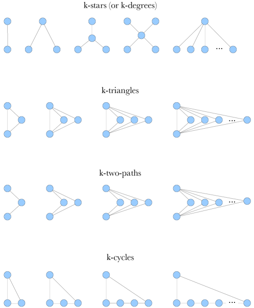
Figure 1: Some of the most used sub-graph configurations for undirected graphs (analogous directed versions can be used for digraphs).

In the ERGM context, the intractability of the likelihood makes the use of standard techniques very challenging. The purpose of this paper is to present two new methods for Bayesian model selection for ERGMs. This article is structured as follows. A brief overview of Bayesian model selection theory is given in Section 2. An across-model approach based on a trans-dimensional extension of the exchange algorithm of Caimo and Friel (2011) is presented in Section 3. The issue of the choosing parameters for the proposal distributions involved in the across model moves is addressed by presenting an automatic reversible jump exchange algorithm involving an independence sampler based on a distribution fitting a parametric density approximation to the within-model posterior. This algorithm bears some similarity to that presented in Chapter 6 of Green (2003). We also present an approach to estimate the model evidence based on thermodynamic integration, although it is limited in that it can only be applied to ERGMs with a small number of parameters. This is outlined in Section 4. Three illustrations of how these new methods perform in practice are given in Section 5. Some conclusions are outlined in Section 6. The Bergm package for R (Caimo and Friel, 2012), implements the newly developed methodology in this paper. It is available on the CRAN package repository at http://cran.r-project.org/web/packages/Bergm.

2 Overview of Bayesian model selection

Bayesian model comparison is commonly performed by estimating posterior model probabilities. More precisely, suppose that the competing models can be enumerated and indexed by the set $\{m_{h}:h=1,\dots,H\}$. Suppose data y are assumed to have been generated by model $m_{h}$, the posterior distribution is:

$$p(\bm{\theta}_{h}|\textbf{\em y},m_{h})=\frac{p(\textbf{\em y}|\bm{\theta}_{h},m_{h})\;p(\bm{\theta}_{h}|m_{h})}{p(\textbf{\em y}|m_{h})},$$ (2)

where $p(\textbf{\em y}|\bm{\theta}_{h},m_{h})$ is the likelihood and $p(\bm{\theta}_{h}|m_{h})$ represents the prior distribution of the parameters of model $m_{h}$. The model evidence (or marginal likelihood) for model $m_{h}$,

$$p(\textbf{\em y}|m_{h})=\int_{\bm{\theta}_{h}}p(\textbf{\em y}|\bm{\theta}_{h},m_{h})\;p(\bm{\theta}_{h}|m_{h})\;d\bm{\theta}_{h},$$ (3)

represents the probability of the data y given a certain model $m_{h}$ and is typically impossible to compute analytically. However, the model evidence is crucial for Bayesian model selection since it allows us to make statements about posterior model probabilities. Bayes’ theorem can be written as

$$p(m_{h}|\textbf{\em y})=\frac{p(\textbf{\em y}|m_{h})\;p(m_{h})}{\sum_{1}^{H}p(\textbf{\em y}|m_{h})\;p(m_{h})}.$$ (4)

Based on these posterior probabilities, pairwise comparison of models, $m_{h}$ and $m_{k}$ say, can be summarised by the posterior odds:

$$\frac{p(m_{h}|\textbf{\em y})}{p(m_{k}|\textbf{\em y})}=\frac{p(\textbf{\em y}|m_{h})}{p(\textbf{\em y}|m_{k})}\times\frac{p(m_{h})}{p(m_{k})}.$$ (5)

This equation reveals how the data y through the Bayes factor

$$BF_{hk}=\frac{p(\textbf{\em y}|m_{h})}{p(\textbf{\em y}|m_{k})}$$ (6)

updates the prior odds

$$\frac{p(m_{h})}{p(m_{k})}$$ (7)

to yield the posterior odds. Table 1 displays guidelines which Kass and Raftery (1995) suggest for interpreting Bayes factors.

$BF_{hk}$	Evidence against model $m_{k}$
$1$ to $3$	Not worth more than a bare mention
$3$ to $20$	Positive
$20$ to $150$	Strong
$>150$	Very strong

Table 1: Guidelines for interpreting Bayes factors, following Kass and Raftery (1995).

By treating $p(m_{h}|\textbf{\em y})$ as a measure of the uncertainty of model $m_{h}$, a natural approach for model selection is to choose the most likely $m_{h}$, a posteriori, i.e. the model for which $p(m_{h}|\textbf{\em y})$ is the largest.

Bayesian model averaging (Hoeting et al., 1999) provides a way of summarising model uncertainty in inference and prediction. After observing the data y one can predict a possible future outcome $\textbf{\em y}^{*}$ by calculating an average of the posterior distributions under each of the models considered, weighted by their posterior model probability.:

$$p(\textbf{\em y}^{*}|\textbf{\em y})=\sum_{h=1}^{H}p(\textbf{\em y}^{*}|m_{h},\textbf{\em y})p(m_{h}|\textbf{\em y}),$$ (8)

where $p(\textbf{\em y}^{*}|m_{h},\textbf{\em y})$ represents the posterior prediction of $\textbf{\em y}^{*}$ according to model $m_{h}$ and data y.

2.1 Computing Bayes factors

Generally speaking there are two approaches for computing Bayes factors: across-model and within-model estimation. The former strategy involves the use of an MCMC algorithm generating a single Markov chain which crosses the joint model and parameter space so as to sample from

$$p(\bm{\theta}_{h},m_{h}|\textbf{\em y})\propto p(\textbf{\em y}|\bm{\theta}_{h},m_{h})\;p(\bm{\theta}_{h}|m_{h})\;p(m_{h}).$$ (9)

One of the most popular approach used in this context is the reversible jump MCMC algorithm of Green (1995) which is briefly reviewed in Section 2.1.1. Within-model strategies focus on the posterior distribution (2) for each competing model $m_{h}$ separately, aiming to estimate their model evidence (3) which can then be used to calculate Bayes factors (see for example Chib (1995), Chib and Jeliazkov (2001), Neal (2001), Friel and Pettitt (2008), and Friel and Wyse (2012), who present a review of these methods). A within-model approach for estimating model evidence is presented in Section 4.

Across-model approaches have the advantage of avoiding the need for computing the evidence for each competing model by treating the model indicator $m_{h}$ as a parameter, but they require appropriate jumping design to produce computationally efficient and theoretically effective methods. Approximate Bayesian Computation (ABC) likelihood-free algorithms for model choice have been recently introduced by Grelaud et al. (2009) in order to allow the computation of the posterior probabilities of the models under competition. However these methods rely on proposing parameter values from the prior distributions which can differ very much from the posterior distribution and this can therefore affect the estimation process. Variational approaches to Bayesian model selection have been presented by McGrory and Titterington (2006) in the context of finite mixture distributions.

2.1.1 Reversible jump MCMC

The Reversible Jump MCMC (RJMCMC) algorithm is a flexible technique for model selection introduced by Green (1995) which allows simulation from target distributions on spaces of varying dimension. In the reversible jump algorithm, the Markov chain “jumps” between parameter subspaces (models) of differing dimensionality, thereby generating samples from the joint distribution of parameters and model indices.

To implement the algorithm we consider a countable collection of candidate models, $\{m_{k}:k=1,\dots,K\}$, each having an associated vector of parameters $\bm{\theta}_{k}$ of dimension $D_{k}$ which typically varies across models. We would like to use MCMC to sample from the joint posterior (9).

In order to jump from $(\bm{\theta}_{k},m_{k})$ to $(\bm{\theta}_{h},m_{h})$, one may proceed by generating a random vector u from a distribution $g$ and setting $(\bm{\theta}_{h},m_{h})=f_{kh}((\bm{\theta}_{k},m_{k}),\textbf{\em u})$. Similarly to jump from $(\bm{\theta}_{h},m_{h})$ to $(\bm{\theta}_{k},m_{k})$ we have $(\bm{\theta}_{k},m_{k})=f_{hk}((\bm{\theta}_{h},m_{h}),\textbf{\em u}^{*})$ where $u^{*}$ is a random vector from a distribution $g^{*}$ and $f_{hk}$ is some deterministic function. However reversibility is only guaranteed when the parameter transition function $f_{kh}$ is a diffeomorphism, that is, both a bijection and its differential invertible. A necessary condition for this to apply is the so-called “dimension matching”: $dim(\bm{\theta}_{k})+dim(\textbf{\em u})=dim(\bm{\theta}_{h})+dim(\textbf{\em u}^{*})$ (where $dim(\cdot)$ stands for “dimension of”). In this case the acceptance probability can be written as:

$$\min\left\{1,\frac{p(\bm{\theta}_{h},m_{h}|\textbf{\em y})}{p(\bm{\theta}_{k},m_{k}|\textbf{\em y})}\frac{p(m_{h}\rightarrow m_{k})}{p(m_{k}\rightarrow m_{h})}\frac{g^{*}(\textbf{\em u}^{*})}{g(\textbf{\em u})}|J|\right\}$$ (10)

where $p(m_{h}\rightarrow m_{k})$ is the probability of jumping from model $m_{h}$ to model $m_{k}$, and $|J|$ is the Jacobian resulting from the transformation from $((\bm{\theta}_{k},m_{k}),\textbf{\em u})$ to $((\bm{\theta}_{h},m_{h}),\textbf{\em u}^{*})$.

Mixing is crucially affected by the choice of the parameters of the jump proposal distribution $g$ and this is one of the fundamental difficulties that makes RJMCMC often hard to use in practice (Brooks et al., 2003).

3 Reversible jump exchange algorithm

In the ERGM context, RJMCMC techniques cannot be used straightforwardly because the likelihood normalizing constant $z(\bm{\theta})$ in (1) cannot be computed analytically.

Here we present an implementation of an RJMCMC approach for ERGMs based on an extension of the exchange algorithm of Murray et al. (2006) developed for exponential random graph models. The algorithm in Caimo and Friel (2011) allows sampling within model $m_{h}$ from the following augmented distribution:

$$p(\bm{\theta}^{\prime}_{h},\textbf{\em y}^{\prime},\bm{\theta}_{h}|\textbf{\em y},m_{h})\propto p(\textbf{\em y}|\bm{\theta}_{h},m_{h})p(\bm{\theta}_{h}|m_{h})h(\bm{\theta}^{\prime}_{h}|\bm{\theta}_{h},m_{h})p(\textbf{\em y}^{\prime}|\bm{\theta}^{\prime}_{h},m_{h})$$ (11)

where $p(\textbf{\em y}|\bm{\theta}_{h},m_{h})$ and $p(\textbf{\em y}^{\prime}|\bm{\theta}^{\prime}_{h},m_{h})$ are respectively the original likelihood defined on the observed data y and the augmented likelihood defined on simulated data $\textbf{\em y}^{\prime}$, $p(\bm{\theta}_{h}|m_{h})$ is the parameter prior and $h(\bm{\theta}^{\prime}_{h}|\bm{\theta}_{h},m_{h})$ is any arbitrary proposal distribution for $\bm{\theta}^{\prime}_{h}$. Marginalising (11) over $\bm{\theta}^{\prime}_{h}$ and $\textbf{\em y}^{\prime}$ yields the posterior of interest $p(\bm{\theta}_{h}|\textbf{\em y},m_{h})$. Note that the simulation of a network $\textbf{\em y}^{\prime}$ from $p(\cdot|\bm{\theta}^{\prime}_{h},m_{h})$ is accomplished by a standard MCMC algorithm (Hunter et al., 2008) as perfect sampling has not yet been developed for ERGMs.

Auxiliary variable methods for intractable likelihood models, such as the exchange algorithm, have not been used in a trans-dimensional setting before. In order to propose to move from $(\bm{\theta}_{k},m_{k})$ to $(\bm{\theta}^{\prime}_{h},m^{\prime}_{h})$, the algorithm (11) can be extended to sample from:

$$p(\bm{\theta}^{\prime}_{h},\bm{\theta}_{k},m^{\prime}_{h},m_{k},\textbf{\em y}^{\prime}|\textbf{\em y})\propto p(\textbf{\em y}|\bm{\theta}_{k},m_{k})p(\bm{\theta}_{k}|m_{k})p(m_{k})h(\bm{\theta}^{\prime}_{h},m^{\prime}_{h}|\bm{\theta}_{k},m_{k})p(\textbf{\em y}^{\prime}|\bm{\theta}^{\prime}_{h},m^{\prime}_{h})$$ (12)

where $p(\textbf{\em y}|\bm{\theta}_{k},m_{k})$ and $p(\textbf{\em y}^{\prime}|\bm{\theta}^{\prime}_{h},m^{\prime}_{h})$ are the two likelihood distributions for the data y under model $m_{k}$ and the auxiliary data $\textbf{\em y}^{\prime}$ under the competing model $m^{\prime}_{h}$ respectively, $p(\bm{\theta}_{k}|m_{k})$ and $p(m_{k})$ are the priors for the parameter $\bm{\theta}_{k}$ and the respective model $m_{k}$ and $h(\bm{\theta}^{\prime}_{h},m^{\prime}_{h}|\bm{\theta}_{k},m_{k})$ is some jump proposal distribution. Analogously as before, the marginal of (12) for $\bm{\theta}^{\prime}_{h}$ and $m^{\prime}_{h}$ is the distribution of interest (9).

Suppose that the current state of the chain is $(\bm{\theta}_{k},m_{k})$ and let us propose a move to $(\bm{\theta}^{\prime}_{h},m^{\prime}_{h})$. The Metropolis-Hastings ratio for accepting the whole move is:

$$\begin{split}&\frac{p(\textbf{\em y}^{\prime}|\bm{\theta}_{k},m_{k})}{p(\textbf{\em y}|\bm{\theta}_{k},m_{k})}\frac{p(\textbf{\em y}|\bm{\theta}^{\prime}_{h},m^{\prime}_{h})}{p(\textbf{\em y}^{\prime}|\bm{\theta}^{\prime}_{h},m^{\prime}_{h})}\frac{p(\bm{\theta}^{\prime}_{h}|m^{\prime}_{h})}{p(\bm{\theta}_{k}|m_{k})}\frac{p(m^{\prime}_{h})}{p(m_{k})}\frac{h(\bm{\theta}_{k},m_{k}|\bm{\theta}^{\prime}_{h},m^{\prime}_{h})}{h(\bm{\theta}^{\prime}_{h},m^{\prime}_{h}|\bm{\theta}_{k},m_{k})}=\\ &\frac{q_{\bm{\theta}_{k},m_{k}}(\textbf{\em y}^{\prime})}{q_{\bm{\theta}_{k},m_{k}}(\textbf{\em y})}\frac{q_{\bm{\theta}^{\prime}_{h},m^{\prime}_{h}}(\textbf{\em y})}{q_{\bm{\theta}^{\prime}_{h},m^{\prime}_{h}}(\textbf{\em y}^{\prime})}\frac{p(\bm{\theta}^{\prime}_{h}|m^{\prime}_{h})}{p(\bm{\theta}_{k}|m_{k})}\frac{p(m^{\prime}_{h})}{p(m_{k})}\frac{h(\bm{\theta}_{k},m_{k}|\bm{\theta}^{\prime}_{h},m^{\prime}_{h})}{h(\bm{\theta}^{\prime}_{h},m^{\prime}_{h}|\bm{\theta}_{k},m_{k})}\times\frac{z(\bm{\theta}_{k})}{z(\bm{\theta}_{k})}\frac{z(\bm{\theta}^{\prime}_{h})}{z(\bm{\theta}^{\prime}_{h})}\end{split}$$

where $q_{\bm{\theta}_{k},m_{k}}(\textbf{\em y})$ indicates the unnormalised likelihood of $p(\textbf{\em y}|\bm{\theta}_{k},m_{k})$ (and so forth for the other functions $q(\cdot)$). Note that the normalising constants corresponding to the unnormalised likehoods cancel. Therefore the ratio above is free of any dependence on normalising constants and so can be evaluated.

The issue with this method is that tuning the jump proposals $h(\cdot)$ in a sensible way so as to get a reasonable mixing can be difficult and automatic choice of jump parameters (Brooks et al., 2003) does not apply in this context due to the intractability of the likelihood distribution.

3.1 Pilot-tuned RJ exchange algorithm

We now consider nested models or models differing by at most one variable. In this case, the move from $(\bm{\theta}_{k},m_{k})$ to a larger model $(\bm{\theta}^{\prime}_{k+1},m^{\prime}_{k+1})$ such that $dim(m^{\prime}_{k+1})=dim(m_{k})+1$ can be done by proposing the transformation $(\bm{\theta}^{\prime}_{k+1},m^{\prime}_{k+1})=((\bm{\theta}_{k},\theta^{\prime}_{k+1}),m_{k+1})$ where the $(k+1)$-th parameter value $\theta^{\prime}_{k+1}$ is generated from some distribution $g_{k+1}$ and then accepting the move with the following probability:

$$\alpha=\min\left\{1,\frac{q_{\bm{\theta}_{k},m_{k}}(\textbf{\em y}^{\prime})}{q_{\bm{\theta}_{k},m_{k}}(\textbf{\em y})}\frac{q_{\bm{\theta}^{\prime}_{k+1},m^{\prime}_{k+1}}(\textbf{\em y})}{q_{\bm{\theta}^{\prime}_{k+1},m^{\prime}_{k+1}}(\textbf{\em y}^{\prime})}\frac{p(\bm{\theta}^{\prime}_{k+1}|m^{\prime}_{k+1})}{p(\bm{\theta}_{k}|m_{k})}\frac{p(m^{\prime}_{k+1})}{p(m_{k})}\frac{1}{g_{k+1}(\theta^{\prime}_{k+1})}\frac{h(m_{k}|m^{\prime}_{k+1})}{h(m^{\prime}_{k+1}|m_{k})}\right\}.$$

The reverse move is accepted with a probability based upon the reciprocal of the acceptance ratio (3.1). The jump within the same model $m_{k}$ is accepted with the following probability:

$$\alpha=\min\left\{1,\frac{q_{\bm{\theta}_{k},m_{k}}(\textbf{\em y}^{\prime})}{q_{\bm{\theta}_{k},m_{k}}(\textbf{\em y})}\frac{q_{\bm{\theta}^{\prime}_{k},m^{\prime}_{k}}(\textbf{\em y})}{q_{\bm{\theta}^{\prime}_{k},m^{\prime}_{k}}(\textbf{\em y}^{\prime})}\frac{p(\bm{\theta}^{\prime}_{k}|m^{\prime}_{k})}{p(\bm{\theta}_{k}|m_{k})}\frac{p(m^{\prime}_{k})}{p(m_{k})}\frac{g(\bm{\theta}_{k})}{g(\bm{\theta}^{\prime}_{k})}\right\}.$$

3.2 Auto-RJ exchange algorithm

Finding suitable parameter values for the proposals for the jump move between models is a very challenging task and is vital in order to ensure adequate mixing of the trans-dimensional Markov chain. In practice, tuning the parameters of the proposals for the trans-dimensional move is very difficult without any information about the posterior density covariance structure. In our experience, in the context of ERGMs, it is extremely difficult to pilot tune a RJMCMC approach to yield adequate mixing rates, rendering this approach impractical for most situations. A possible approach would be to use an independence sampler which does not depend on the current state of the MCMC chain but fits a parametric density approximation to the within-model posterior distribution so as to have an acceptance rate as high as possible.

In this spirit, we can propose to jump from $(\bm{\theta}_{k},m_{k})$ to $(\bm{\theta}^{\prime}_{h},m^{\prime}_{h})$ using the following jump proposals:

$$h(\bm{\theta}^{\prime}_{h},m^{\prime}_{h}|\bm{\theta}_{k},m_{k})=w(\bm{\theta}^{\prime}_{h}|m^{\prime}_{h})\;h(m^{\prime}_{h}|m_{k})$$ (13)

where $h(m_{k}|m^{\prime}_{h})$ represents a between-model jump proposal from model $m_{k}$ to model $m^{\prime}_{h}$ and $w(\bm{\theta}^{\prime}_{h}|m^{\prime}_{h})$ is the within-model jump proposal for model $m^{\prime}_{h}$. As remarked above, the within-model proposals require careful tuning. Posterior density approximations such as standard distributions with parameters determined by the moments of a sample drawn from (12) can be used as within model proposals for each competing model. Indeed this is similar to the type of strategy outlined in Chapter 6 of Green (2003). For example, $w(\bm{\theta}_{l}|m_{l})$ can be a normal distribution $\mathcal{N}(\hat{\bm{\mu}}_{l},\hat{\bm{\Sigma}}_{l})$ where $\hat{\bm{\mu}}_{l}$ and $\hat{\bm{\Sigma}}_{l}$ are the posterior mean and covariance estimates for each model $m_{l}$. In our experience the choice of normal proposals appear to fit quite well in most of the examples we looked at, although using $t-$distributions may be more robust to heavier tails in the posterior.

The algorithm can be therefore summarized in two steps: the first step (offline) is used to sample from the posterior (11) of each model $m_{l}$ and to estimate the parameters $\hat{\bm{\mu}}_{l}$ and $\hat{\bm{\Sigma}}_{l}$ of the within-model jump proposal; the second step (online) carries out the MCMC computation of (12).

The algorithm can be written in the following concise way:

OFFLINE RUN

(0) Estimation of $p(\bm{\theta}_{l}|\textbf{\em y},m_{l})\;$ for $l=1,\dots,H$
i Set $\hat{\bm{\mu}}_{l}={\mathbb{E}}(\bm{\theta}_{l}|\textbf{\em y},m_{l})$ and $\hat{\bm{\Sigma}}_{l}=Cov(\bm{\theta}_{l}|\textbf{\em y},m_{l})$
ii Use $w(\bm{\theta}_{l}|m_{l})\sim\mathcal{N}(\hat{\bm{\mu}}_{l},\hat{\bm{\Sigma}}_{l})$ as within-model jump proposals, when proposing to jump to model $m_{l}$

ONLINE RUN

(1.1) Gibbs update of $(m^{\prime}_{h},\bm{\theta}^{\prime}_{h},\textbf{\em y}^{\prime})$
i Propose $m^{\prime}_{h}$ from the prior $p(\cdot)$
ii Propose $\bm{\theta}^{\prime}_{h}$ with probability $w(\cdot|\hat{\bm{\mu}}_{h},\hat{\bm{\Sigma}}_{h})$
iii Draw $\textbf{\em y}^{\prime}$ from $p(\cdot|\bm{\theta}^{\prime}_{h},m^{\prime}_{h})$

(1.2) Accept the jump from $(\bm{\theta}_{k},m_{k})$ to $(\bm{\theta}^{\prime}_{h},m^{\prime}_{h})$ with probability:

$$\min\left\{1,\frac{q_{\bm{\theta}_{k},m_{k}}(\textbf{\em y}^{\prime})}{q_{\bm{\theta}_{k},m_{k}}(\textbf{\em y})}\frac{q_{\bm{\theta}^{\prime}_{h},m^{\prime}_{h}}(\textbf{\em y})}{q_{\bm{\theta}^{\prime}_{h},m^{\prime}_{h}}(\textbf{\em y}^{\prime})}\frac{p(\bm{\theta}^{\prime}_{h}|m^{\prime}_{h})}{p(\bm{\theta}_{k}|m_{k})}\frac{p(m^{\prime}_{h})}{p(m_{k})}\frac{w(\bm{\theta}_{k}|\hat{\bm{\mu}}_{k},\hat{\bm{\Sigma}}_{k})}{w(\bm{\theta}^{\prime}_{h}|\hat{\bm{\mu}}_{h},\hat{\bm{\Sigma}}_{h})}\frac{h(m_{k}|m^{\prime}_{k})}{h(m^{\prime}_{h}|m_{k})}\right\}.$$

4 Estimating model evidence

In this section we present a within-model approach for estimating the evidence $p(\textbf{\em y})$ (For ease of notation, we will omit the conditioning on the model indicator $m_{l}$). The aim is to provide a useful method for low-dimensional models to use as a “ground-truth” reference to compare with the reversible jump exchange algorithm. The method follows from noticing that for any parameter $\bm{\theta}^{\star}$, equation (2) implies that:

$$p(\textbf{\em y})=p(\textbf{\em y}|\bm{\theta}^{\star})\frac{p(\bm{\theta}^{\star})}{p(\bm{\theta}^{\star}|\textbf{\em y})}=\frac{q_{\bm{\theta}^{\star}}(\textbf{\em y})}{z(\bm{\theta}^{\star})}\frac{p(\bm{\theta}^{\star})}{p(\bm{\theta}^{\star}|\textbf{\em y})}.$$ (14)

This is also the starting point for Chib’s method for estimating the evidence (Chib, 1995). Typically $\bm{\theta}^{\star}$ is chosen as a point falling in the high posterior probability region so as to increase the accuracy of the estimate. To estimate (14), the calculation of the intractable likelihood normalizing constant $z(\bm{\theta}^{\star})$ and an estimate of the posterior density $p(\bm{\theta}^{\star}|\textbf{\em y})$ are required.

Estimating $z(\bm{\theta}^{\star})$ via path sampling

The first problem can be tackled using a path sampling approach (Gelman and Meng, 1998). Consider introducing an auxiliary variable $t\in[0,1]$. We consider the following distribution:

$$p_{t}(\textbf{\em y}|\bm{\theta})=p(\textbf{\em y}|\bm{\theta})^{t}=p(\textbf{\em y}|\bm{\theta}t)=\frac{q_{\bm{\theta}t}(\textbf{\em y})}{z(\bm{\theta}t)}=\frac{\exp\{(\bm{\theta}t)^{T}s(\textbf{\em y})\}}{\sum_{\textbf{\em y}\in\mathcal{Y}}\exp\{(\bm{\theta}t)^{T}s(\textbf{\em y})\}}.$$ (15)

Taking logarithms and differentiating $\log\left[z(\bm{\theta}^{\star}t)\right]$ with respect to $t$ yields:

$$\frac{d}{dt}\log\left[z(\bm{\theta}^{\star}t)\right] =\frac{1}{z(\bm{\theta}^{\star}t)}\frac{d}{dt}z(\bm{\theta}^{\star}t)$$

$$=\frac{1}{z(\bm{\theta}^{\star}t)}\frac{d}{dt}\sum_{\textbf{\em y}\in\mathcal{Y}}\exp\left\{(\bm{\theta}^{\star}t)^{T}s(\textbf{\em y})\right\}$$

$$=\frac{1}{z(\bm{\theta}^{\star}t)}\sum_{\textbf{\em y}\in\mathcal{Y}}\left[\bm{\theta}^{\star T}s(\textbf{\em y})\right]\exp\left\{(\bm{\theta}^{\star}t)^{T}s(\textbf{\em y})\right\}$$

$$=\sum_{\textbf{\em y}\in\mathcal{Y}}\left[\bm{\theta}^{\star T}s(\textbf{\em y})\right]\;p(\textbf{\em y}|\bm{\theta}^{\star}t)$$

$$={\mathbb{E}}_{\textbf{\em y}|\bm{\theta}^{\star}t}\left[\bm{\theta}^{\star T}s(\textbf{\em y})\right].$$ (16)

where ${\mathbb{E}}_{\textbf{\em y}|\bm{\theta}^{\star}t}$ denotes the expectation with respect to the sampling distribution $p(\textbf{\em y}|\bm{\theta}^{\star}t)$. Therefore integrating (16) from $0$ to $1$ gives:

$$\log\left\{\frac{z(\bm{\theta}^{\star})}{z(\bf 0)}\right\}=\int\limits_{0}^{1}{\mathbb{E}}_{\textbf{\em y}|\bm{\theta}^{\star}t}[\bm{\theta}^{\star T}s(\textbf{\em y})]\;dt.$$

Now if we choose a discretisation of the variable $t$ such that $t_{0}=0<\dots<t_{i}<\dots<t_{I}=1$, this leads to the following approximation:

$$\log\left\{\frac{z(\bm{\theta}^{\star})}{z(\bf 0)}\right\}\approx\sum\limits_{i=0}^{I-1}(t_{i+1}-t_{i})\;\left(\frac{{\mathbb{E}}_{\textbf{\em y}|\bm{\theta}^{\star}t_{i}}[\bm{\theta}^{\star T}s(\textbf{\em y})]+{\mathbb{E}}_{\textbf{\em y}|\bm{\theta}^{\star}t_{i+1}}[\bm{\theta}^{\star T}s(\textbf{\em y})]}{2}\right).$$ (17)

Remember that $z(\mathbf{0})$ is analytically available and it is equal to $2^{\binom{n}{2}}$ i.e. the number of possible graphs on the $n$ nodes of the observed network. In terms of computation, ${\mathbb{E}}_{\textbf{\em y}|\bm{\theta}^{\star}t_{i}}[\bm{\theta}^{\star T}s(\textbf{\em y})]$ can be easily estimated using the same procedures used for simulating auxiliary data from the ERGM likelihood. Hence in (17) two types of error emerge: discretisation of (14) and Monte Carlo error due to the simulation approximation of ${\mathbb{E}}_{\textbf{\em y}|\bm{\theta}^{\star}t_{i}}[\bm{\theta}^{\star T}s(\textbf{\em y})]$. The path of $t_{i}$’s is important for the efficiency of the evidence estimate. For example, we can choose a path of the type $t_{i}=(1/I)^{c}$ where $c$ is some tuning constant: for $c=1$ we have equal spacing of the $I$ points in the interval $[0,1]$, for $c>1$ we have that the $t_{i}$’s are chosen with high frequency close to $0$ and for $0<c<1$ we have that the $t_{i}$’s are chosen with high frequency close to $1$.

Estimating $p(\bm{\theta}^{\star}|\textbf{\em y})$

A sample from the posterior $p(\bm{\theta}|\textbf{\em y})$ can be gathered (via the exchange algorithm, for example) and used to calculate a kernel density estimate of the posterior probability at the point $\bm{\theta}^{\star}$. In practice, because of the curse of dimensionality, this implies that the method cannot be used, for models with greater than $5$ parameters. In this paper we used the fast and easy to use np package for R (Hayfield and Racine, 2008) to perform a nonparametric density estimation of the posterior $p(\bm{\theta}^{\star}|\textbf{\em y})$.

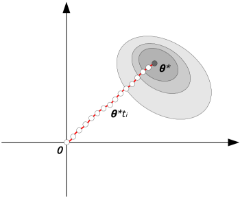
Figure 2: Path sampling: for each $\bm{\theta}^{\star}$ we estimate $z(\bm{\theta}^{\star})$ via path sampling using the expected network statistics simulated from some points $\bm{\theta}^{\star}t_{i}$ along the line connecting $\bf 0$ to $\bm{\theta}^{\star}$.

5 Applications

5.1 Gahuku-Gama system

The Gahuku-Gama system (Read, 1954) of the Eastern Central Highlands of New Guinea was used by Hage and Harary (1984) to describe an alliance structure among 16 sub-tribes of Eastern Central Highlands of New Guinea (Figure 3). The system has been split into two network: the “Gamaneg” graph for antagonistic (“hina”) relations and the “Gamapos” for alliance (“rova”) relations. An important feature of these structures is the fact that the enemy of an enemy can be either a friend or an enemy.

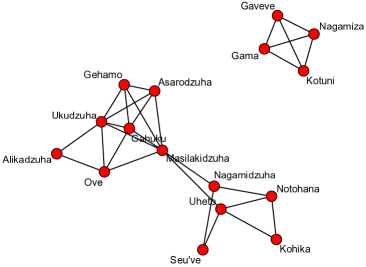
Figure 3: Gahuku-Gama system graphs: Gamaneg (top) and Gamapos (bottom).

5.1.1 Gamaneg

We first focus on the Gamaneg network by using the 3 competing models specified in Table 2 using the following network statistics:

edges	$\sum_{i<j}y_{ij}$
triangles	$\sum_{i<j<k}y_{jk}y_{ik}y_{ij}$
4-cycle	$\sum_{i<j<l<k}y_{ij}y_{jl}y_{lk}y_{ki}$

We are interested to understand if the transitivity effect expressed by triad closure (triangle) and 4-cycle which is a closed structure that permits to measure the dependence between two edges that do not share a node (Pattison and Robins, 2002).

Model $m_{1}$	$\textbf{\em y}\sim$ edges
Model $m_{2}$	$\textbf{\em y}\sim$ edges $+$ triangles
Model $m_{3}$	$\textbf{\em y}\sim$ edges $+$ triangles $+$ 4-cycle

Table 2: Competing models.

Both the pilot-tuned RJ and auto-RJ exchange algorithms were run for $100,000$ iterations using very flat normal parameter priors $p(\bm{\theta}_{l}|m_{l})\sim\mathcal{N}(0,100\textbf{\em I}_{l})$ for each model $m_{l}$ where $\textbf{\em I}_{l}$ is the identity matrix of size equal to the number of dimensions of model $m_{l}$ and $3,000$ iterations for the auxiliary network simulation. The proposal distributions of the pilot-tuned RJ were empirically tuned so as to get reasonable acceptance rates for each competing model. The offline step of the auto-RJ consisted of gathering an approximate sample from $p(\bm{\theta}|\textbf{\em y})$ and then estimating the posterior moments $\hat{\bm{\mu}}_{l}$ and $\hat{\bm{\Sigma}}_{l}$ for each of the three models. The exchange algorithm was run for $1,000\times D_{l}$ iterations (discarding the first $100\times D_{l}$ iterations as burn-in) where $D_{l}$ is the dimension of the $l$-th model using the population MCMC approach described in Caimo and Friel (2011). The accuracy of the estimates $\hat{\bm{\mu}}_{l}$ and $\hat{\bm{\Sigma}}_{l}$ depends on the number of iterations of the auto-RJ offline run. In this example, the above number of iterations $1,000\times D_{l}$ of has been empirically shown to be sufficient for each competing model $m_{l}$. In this example and all the examples that follow we use uniform model prior and uniform between-model jump proposals. Tables 3 and 4 report the posterior parameter estimates of the model selected for the pilot-tuned RJ and auto-RJ. From these tables we can see that the pilot-tuned RJ sampler exhibits poor within-model mixing with respect to the good mixing of the auto-RJ sampler. This greatly affected the convergence of the pilot-tuned RJ leading to very poor posterior estimates. Figure 4 shows the results from the pilot-tuned RJ, namely, model posterior diagnostic plots and the parameter posterior diagnostic plots. Figure 5 shows the same plots from auto-RJ. Between-model and within-model acceptance rates (reported in Table 4) are calculated as the proportions of accepted moves from $(\bm{\theta}_{k},m_{k})$ to model $(\bm{\theta}^{\prime}_{h},m^{\prime}_{h})$ for each $k:k\neq h$ and when $k=h$, respectively. The mixing of the auto-RJ algorithm within each model is faster than the pilot-tuned RJ algorithm due to the good approximation to the posterior distribution. The pilot-tuned algorithm took about 24 minutes to complete the estimation and the auto-RJ took about 31 minutes (including the offline step).

	Pilot-tuned RJ		Auto-RJ
Parameter	Post. Mean	Post. Sd.	Post. Mean	Post. Sd.
Model $m_{1}$
$\theta_{1}$ (edge)	-1.15	0.21	-1.15	0.21
Model $m_{2}$
$\theta_{1}$ (edge)	-0.97	0.36	-0.96	0.37
$\theta_{2}$ (triangle)	-0.31	0.41	-0.29	0.37
Model $m_{3}$
$\theta_{1}$ (edge)	-0.98	0.51	-1.15	0.37
$\theta_{2}$ (triangle)	-0.76	0.47	-0.31	0.42
$\theta_{3}$ (4-cycle)	-0.05	0.12	0.02	0.17

Table 3: Summary of posterior parameter estimates.

Within-model	Pilot-tuned RJ	Auto-RJ
Model $m_{1}$	$0.14$	$0.62$
Model $m_{2}$	$0.11$	$0.42$
Model $m_{3}$	$0.00$	$0.48$
Between-model	$0.07$	$0.04$

Table 4: Acceptance rates.

	Pilot-tuned RJ	Auto-RJ
$\widehat{BF}_{1,2}$	$14.46$	$21.68$
$\widehat{BF}_{1,3}$	$1506.43$	$1425.77$
$\widehat{p}(m_{1}|\textbf{\em y})$	$0.93$	$0.95$
$\widehat{p}(m_{2}|\textbf{\em y})$	$0.06$	$0.04$
$\widehat{p}(m_{3}|\textbf{\em y})$	$0.01$	$0.01$

Table 5: Bayes factor and posterior model probability estimates.

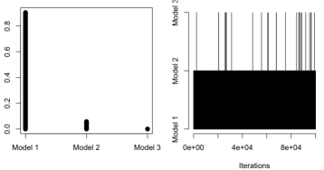
Figure 4: Pilot-tuned RJ exchange algorithm output: posterior model probabilities (top) and posterior parameter probabilities for model $m_{1}$ (bottom).

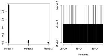
Figure 5: Auto-RJ exchange algorithm output: posterior model probabilities (top) and posterior parameter probabilities for model $m_{1}$ (bottom).

In terms of calculating the evidence based on path sampling, Figure 6 shows the behaviour of ${\mathbb{E}}_{\textbf{\em y}|\bm{\theta}^{\star}t}\left[\bm{\theta}^{\star T}s(\textbf{\em y})\right]$ for $50$ equally-spaced path points $t_{i}$ from 0 to 1. The larger the number of temperatures $I$ and the number of simulated networks, the more precise the estimate of the likelihood normalizing constant and the greater the computing effort. In this example we estimated (16) using $100$ path points and sampling $500$ network statistics for each of them. In this case, this setup has been empirically shown to be sufficiently accurate. We set $c$ to be equal to 1 for all the models. However different choices for $c$ do not seem to have a big influence on the estimation results if $I$ is large enough.

Figure 6: ${\mathbb{E}}[\bm{\theta}^{\star T}s(\textbf{\em y})]$ estimated from a ladder of 50 equally-spaced path points.

A nonparametric density estimation of $p(\bm{\theta}|\textbf{\em y})$ for each competing model was implemented using approximate posterior samples gathered from the output of the exchange algorithm. Bayes Factor estimates for different sample sizes (which are increasing with the number of model dimension) are reported in Table 6. The results are consistent with the ones obtained by RJ exchange algorithm displayed in Table 5. In particular it is possible to observe that as the sample sizes increases the Bayes Factor estimates tend to get closer to the Bayes Factor estimate obtained by the RJ exchange algorithm. The evidence-based approach took about a few seconds to estimate model evidence for $m_{1}$ and $m_{2}$ and about 6 minutes for model $m_{3}$ using the biggest sample sizes displayed in Table 6.

	Sample sizes
Model $m_{1}$	$100$	$500$	$1,000$	$5,000$
Model $m_{2}$	$150$	$750$	$1,500$	$7,500$
Model $m_{3}$	$200$	$1,000$	$2,000$	$10,000$
$\widehat{BF}_{1,2}$	$18.83$	$18.72$	$18.84$	$19.09$
$\widehat{BF}_{1,3}$	$1029.67$	$1324.61$	$1363.91$	$1390.08$

Table 6: Bayes Factor estimates for increasing values of sample sizes used for the posterior density estimation.

The estimates of the Bayes Factors can be interpreted using the guidelines of Kass and Raftery (1995), Table 1, leading to the conclusion that the Bayes Factor estimates obtained suggest that there is positive/strong evidence in favour of model $m_{1}$ which is the one including the number of edges against the other two competing models. Thus in this case the only strong effect of the antagonistic structure of the Gahuku-Gama tribes is represented by the low edge density.

5.1.2 Gamapos

In this second example, we considered the same competing models of Table 2. In this case it turned out that the pilot-tuned RJ exchange algorithm was very difficult to tune, being very sensitive to the choice of the parameters of jump proposal. We used the auto-RJ exchange algorithm with the same set-up of the previous example. The output from auto-RJ exchange algorithm is displayed in Figure 7 and the parameter posterior estimates in Table 7.

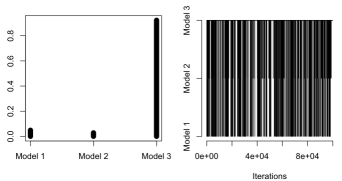
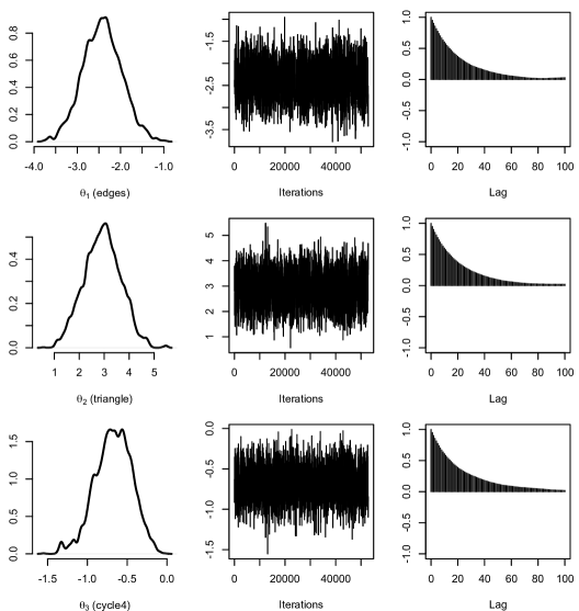
Figure 7: Auto-RJ exchange algorithm output: posterior model probabilities (top) and posterior parameter probabilities for model $m_{3}$ (bottom).

Parameter	Post. Mean	Post. Sd.
Model $m_{3}$ (within-model acc. rate: $0.3$)
$\theta_{1}$ (edge)	-2.41	0.45
$\theta_{2}$ (triangle)	2.91	0.71
$\theta_{3}$ (4-cycle)	-0.66	0.22
Model $m_{1}$ (within-model acc. rate: $0.64$)
$\theta_{1}$ (edge)	-1.15	0.20
Model $m_{2}$ (within-model acc. rate: $0.3$)
$\theta_{1}$ (edge)	-1.69	0.35
$\theta_{2}$ (triangle)	0.48	0.20
Between-model acc. rate: $0.03$

Table 7: Summary of posterior parameter estimates and acceptance rates.

Figure 8: ${\mathbb{E}}[\bm{\theta}^{\star T}s(\textbf{\em y})]$ estimated from a ladder of 50 equally-spaced path points.

We also calculated the evidence for each models following the same setup of the Gamaneg example. Figure 8 shows the behaviour of ${\mathbb{E}}_{\textbf{\em y}|\bm{\theta}^{\star}t}\left[\bm{\theta}^{\star T}s(\textbf{\em y})\right]$ for $50$ equally-spaced path points $t_{i}$ from 0 to 1. Table 8 reports the Bayes Factor estimates of the auto-RJ exchange algorithm and evidence-based method using the biggest sample sizes used for the posterior density estimation of the previous example. From this one can conclude that there is positive/strong support for model $m_{3}$.

	Auto-RJ algorithm	Evidence-based method
$BF_{3,1}$	$17.83$	$19.31$
$BF_{3,2}$	$34.81$	$32.82$

Table 8: Bayes factors estimates.

In the Gamapos network the transitivity and the 4-cycle structure are important features of the network. The tendency to a low density of edges and 4-cycles expressed by the negative posterior mean of the first and third parameters is balanced by a propensity for local triangles which gives rise to the formation of small well-defined alliances.

We remark that both examples should be considered from a pedagogical viewpoint, and not from a solely applied perspective. However it is interesting that although both networks are defined on the same node set, the model selection procedures for each example lead to different models having highest probability, a posteriori. It is also important to note that model $m_{2}$ is known to be a degenerate model (see Jonasson (1999), Butts (2011), and Shalizi and Rinaldo (2011)) as it tends to place almost all probability mass on extreme graphs under almost all values of the parameters. For this reason model $m_{2}$ is unrealistic for real-world networks. Indeed, it may be suspected that model $m_{3}$ is potentially problematic, however the asymptotic properties of this model has not yet been studied. Our Bayesian model choice procedures agree with the previous knowledge of $m_{2}$, as outlined above, in the sense that very little posterior probability is assigned to model $m_{2}$ in both the examples above. One may view this as a useful check of the reliability of the algorithm.

5.2 Collaboration between Lazega’s lawyers

The Lazega network data collected by Lazega (2001) and displayed in Figure 9 represents the symmetrized collaboration relations between the $36$ partners in a New England law firm, where the presence of an edge between two nodes indicates that both partners collaborate with the other.

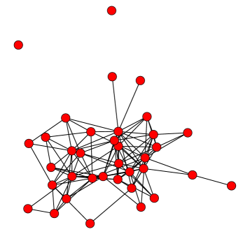
Figure 9: Lazega’s lawyers cowork graph.

5.2.1 Example 1

In this example we want to compare 4 models (Table 9) using the edges, geometrically weighted degrees and geometrically weighted edgewise shared partners (Snijders et al., 2006):

edges	$\sum_{i<j}y_{ij}$
geometrically weighted degree (gwd)	$e^{\phi_{u}}\sum_{k=1}^{n-1}\left\{1-\left(1-e^{-\phi_{u}}\right)^{k}\right\}D_{k}(\textbf{\em y})$
geometrically weighted edgewise	$e^{\phi_{v}}\sum_{k=1}^{n-2}\left\{1-\left(1-e^{-\phi_{v}}\right)^{k}\right\}EP_{k}(\textbf{\em y})$
shared partner (gwesp)

where $\phi_{u}=\log(2)$, $\phi_{v}=\log(2)$, $D_{k}(\textbf{\em y})$ is the number of pairs that have exactly $k$ common neighbours and $EP_{k}(\textbf{\em y})$ is the number of connected pairs with exactly $k$ common neighbours.

Model $m_{1}$	$\textbf{\em y}\sim$ edges
Model $m_{2}$	$\textbf{\em y}\sim$ edges $+$ gwesp($\log(2)$)
Model $m_{3}$	$\textbf{\em y}\sim$ edges $+$ gwesp($\log(2)$) $+$ gwd($\log(2)$)
Model $m_{4}$	$\textbf{\em y}\sim$ edges $+$ gwd($\log(2)$)

Table 9: Competing models.

As happened in the previous example, the pilot-tuned RJ exchange algorithm proved to be ineffective due to the difficulty of the tuning problem. The auto-RJ exchange algorithm was run for $100,000$ iterations using the same flat normal priors of the previous examples and $25,000$ auxiliary iterations for network simulation. The offline run consisted of estimating $\hat{\bm{\mu}}_{l}$ and $\hat{\bm{\Sigma}}_{l}$ for each of the 4 models by using $6,000\times D_{l}$ main iterations (discarding the first $1,000\times D_{l}$ iterations as burnin). The algorithm took about 1 hour and 50 minutes to complete the estimation, the results of which are displayed in Figure 10 and Table 10.

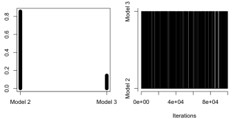
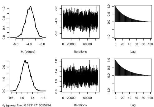
Figure 10: Auto-RJ exchange algorithm output: posterior model probabilities (top) and posterior parameter probabilities for model $m_{2}$ (bottom).

Parameter	Post. Mean	Post. Sd.
Model $m_{2}$ (within-model acc. rate: $0.24$)
$\theta_{1}$ (edge)	-3.93	0.33
$\theta_{2}$ (gwesp($\log(2)$))	1.15	0.16
Model $m_{3}$ (within-model acc. rate: $0.26$)
$\theta_{1}$ (edge)	-4.54	0.56
$\theta_{2}$ (gwesp($\log(2)$))	-1.39	0.23
$\theta_{3}$ (gwd($\log(2)$))	0.79	0.62
Between-model acc. rate: $0.03$

Table 10: Summary of posterior parameter estimates and acceptance rates.

The evidence-based algorithm was carried out using $200$ path points from each of which we sampled $500$ networks. The results are reported in Table 11. The algorithm took 25 seconds to estimate the evidence for model $m_{1}$, 8 minutes for model $m_{2}$, 9 minutes for model $m_{3}$, 1 minute for model $m_{4}$.

Figure 11: ${\mathbb{E}}[\bm{\theta}^{\star T}s(\textbf{\em y})]$ estimated from a ladder of 50 equally-spaced path points.

	Auto-RJ algorithm	Evidence-based method
$BF_{2,1}$	$>10^{6}$	$>10^{6}$
$BF_{2,3}$	$5.72$	$4.65$
$BF_{2,4}$	$>10^{6}$	$>10^{6}$

Table 11: Bayes Factor estimates.

Table 11 displays the Bayes Factor for the comparison between model $m_{2}$ (best model) against the others. There is positive evidence to reject model $m_{3}$ and very strong evidence to models $m_{1}$ and $m_{4}$.

We can therefore conclude that the low density effect expressed by the negative edge parameter combined with the positive transitivity effect expressed by the geometrically weighted edgewise partners parameter are strong structural features not depending on popularity effect expressed by the weighted degrees. These results are in agreement with the findings reported in the literature (see Snijders et al. (2006) and Hunter and Handcock (2006)). However, the advantage of the Bayesian approach used in this paper is that the comparison between competing models is carried out within a fully probabilistic framework while classical approaches test the significativity of each parameter estimate using t-ratios defined as parameter estimate divided by standard error, and referring these to an approximating standard normal distribution as the null distribution.

5.2.2 Example 2

In this example we want to compare the two models specified in Table 12 using the edges, geometrically weighted edgewise shared partners (with $\phi_{v}=\log(2)$) and a set of statistics involving exogenous data based on some nodal attributes available in the Lazega dataset. In particular we consider the following nodal covariates: gender and practice (2 possible values, litigation$=0$ and corporate law$=1$). The covariate statistics are of the form:

$$s(\textbf{\em y},\textbf{\em x})=\sum_{i\neq j}y_{ij}f(x_{i},x_{j})$$

where $f(x_{i},x_{j})$ can either define a “main effect” of a numeric covariate:

$$f(x_{i},x_{j})=x_{i}+x_{j}$$

or a “similarity effect” (or “homophily effect”):

$$f(x_{i},x_{j})=\textbf{\em I}_{\{x_{i}=x_{j}\}}$$

where I is the indicator function.

Model $m_{1}$	Model $m_{2}$
edges	edges
gwesp($\log(2)$)	gwesp($\log(2)$)
practice - homophily	gender - homophily
law-school - homophily	practice - homophily
practice - main effect

Table 12: Competing models.

In this case, due to the high-dimensionality of both the competing models, only the auto-RJ exchange approach was used. The algorithm was run for $50,000$ iterations using the same flat normal priors of the previous examples and $25,000$ auxiliary iterations for network simulation. The offline run consisted of estimating $\hat{\bm{\mu}}_{l}$ and $\hat{\bm{\Sigma}}_{l}$ for each of the 2 models by using $5,000\times D_{l}$ main iterations (discarding the first $1,000\times D_{l}$ iterations as burnin). The algorithm took about 2 hours to complete the estimation, the results of which are displayed in Figure 12 and Table 13.

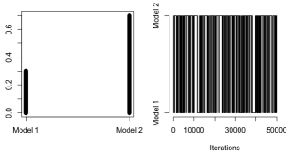
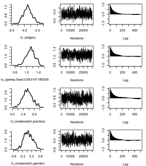
Figure 12: Auto-RJ exchange algorithm output: posterior model probabilities (top) and posterior parameter probabilities for model $m_{2}$ (bottom).

Parameter	Post. Mean	Post. Sd.
Model $m_{2}$ (within-model acc. rate: $0.11$)
$\theta_{1}$ (edge)	$-4.22$	$0.34$
$\theta_{2}$ (gwesp(log(2)))	$1.12$	$0.15$
$\theta_{3}$ (practice - homophily)	$0.55$	$0.17$
$\theta_{4}$ (gender - homophily)	$0.05$	$0.19$
Model $m_{1}$ (within-model acc. rate: $0.13$)
$\theta_{1}$ (edge)	$-4.98$	$0.50$
$\theta_{2}$ (gwesp(log(2)))	$1.14$	$0.17$
$\theta_{3}$ (practice - homophily)	$0.63$	$0.22$
$\theta_{4}$ (gender - homophily)	$0.15$	$0.22$
$\theta_{5}$ (practice - main effect)	$0.20$	$0.08$
Between-model acc. rate: $0.04$

Table 13: Summary of posterior parameter estimates and acceptance rates.

The Bayes Factor for the comparison between model $m_{2}$ (best model) against model $m_{1}$ was around $2.32$ thus implying that there is not strong evidence to reject model $m_{1}$. From the results obtained above, we can state that the collaboration network is enhanced by the practice similarity effect. The first model highlights how the collaboration relations are strongly enhanced by having the same gender or practice. The positive value $\theta_{2}$ in both models indicates the presence of complex transitive effect captured by the edgewise shared partner statistics.

6 Discussion

This paper has explored Bayesian model selection for posterior distributions with intractable likelihood functions. To our knowledge, this work represents a first step in the direction of conducting a Bayesian analysis of model uncertainty for this class of social network models. The methodological developments presented here have applicability beyond exponential random graph models, for example such methodology can be applied to Ising, potts or autologistic models.

We introduced a novel method for Bayesian model selection for exponential random graph models which is based on a trans-dimensional extension of the exchange algorithm for exponential random graph models of Caimo and Friel (2011). This takes the form of an independence sampler making use of a parametric approximation of the posterior in order to overcome the issue of tuning the parameters of the jump proposal distributions and increase within-model acceptance rates. We also note that the methodology may also find use in other recent papers which are also amenable to Bayesian analysis of networks such as Koskinen et al. (2010) for ERGMs in the presence of missing data and Schweinberger and Handcock (2011) who implemented a version of the exchange algorithm adapted to hierarchical ERGMs with local dependence.

This methodology has been illustrated by four examples, and is reproducible using the Bergm package for R (Caimo and Friel, 2012). Additionally we have presented a within-model approach for estimating the model evidence which relies on the path sampling approximation of the likelihood normalizing constant and nonparametric density estimation of the posterior distribution.

The methods described in this paper have their limitations, however. The computational effort required by these algorithms render inference for large networks with hundreds of nodes or models with many parameters, out of range. Moreover, the need to take the final realisation from a finite run Markov chain as an approximate “exact” draw from the intractable likelihood is a practical and pragmatic approach. As yet a perfect sampling algorithm has not been developed for ERGMs, and this would have clear applicability for our algorithms.

References

- Brooks et al. (2003) Brooks, S. P., Giudici, P., and Roberts, G. O. (2003), “Efficient construction of reversible jump Markov chain Monte Carlo proposal distributions (with discussion),” Journal of the Royal Statistical Society, Series B, 65, 3–57.
- Butts (2011) Butts, C. T. (2011), “Bernoulli Graph bounds for general random graphs,” Sociological Methodology, 41, 299–345.
- Caimo and Friel (2011) Caimo, A. and Friel, N. (2011), “Bayesian inference for exponential random graph models,” Social Networks, 33, 41 – 55.
- Caimo and Friel (2012) — (2012), “Bergm: Bayesian exponential random graphs in R,” Tech. rep., University College Dublin, available in e-print format at http://arxiv.org/abs/1201.2770.
- Chib (1995) Chib, S. (1995), “Marginal Likelihood from the Gibbs Output,” Journal of the American Statistical Association, 90, 1313–1321.
- Chib and Jeliazkov (2001) Chib, S. and Jeliazkov, I. (2001), “Marginal Likelihood From the Metropolis-Hastings Output,” Journal of the American Statistical Association, 96, 270–281.
- Erdös and Rényi (1959) Erdös, P. and Rényi, A. (1959), “On random graphs,” Publicationes Mathematicae, 6, 290–297.
- Frank and Strauss (1986) Frank, O. and Strauss, D. (1986), “Markov Graphs,” Journal of the American Statistical Association, 81, 832–842.
- Friel and Pettitt (2008) Friel, N. and Pettitt, A. N. (2008), “Marginal likelihood estimation via power posteriors,” Journal of the Royal Statistical Society, Series B, 70, 589–607.
- Friel and Wyse (2012) Friel, N. and Wyse, J. (2012), “Estimating the statistical evidence – a review,” Statistica Neerlandica, 66, 288–308.
- Gelman and Meng (1998) Gelman, A. and Meng, X. L. (1998), “Simulating normalizing contants: from importance sampling to bridge sampling to path sampling.” Statistical Science, 13, 163–185.
- Green (1995) Green, P. J. (1995), “Reversible jump Markov chain Monte Carlo computation and Bayesian model determination,” Biometrika, 82, 711–732.
- Green (2003) — (2003), “Trans-dimensional Markov chain Monte Carlo,” in Highly Structured Stochastic Systems, Oxford University Press.
- Grelaud et al. (2009) Grelaud, A., Robert, C., Marin, J.-M., Rodolphe, F., and Taly, J.-F. (2009), “ABC likelihood-free methods for model choice in Gibbs random fields,” Bayesian Analysis, 3, 427–442.
- Hage and Harary (1984) Hage, P. and Harary, F. (1984), Structural Models in Anthropology, Cambridge University Press.
- Handcock (2003) Handcock, M. S. (2003), “Assessing Degeneracy in Statistical Models of Social Networks,” Working Paper no.39, Center for Statistics and the Social Sciences, University of Washington.
- Hayfield and Racine (2008) Hayfield, T. and Racine, J. S. (2008), “Nonparametric Econometrics: The np Package,” Journal of Statistical Software, 27.
- Hoeting et al. (1999) Hoeting, J. A., Madigan, D., Raftery, A. E., and Volinsky, C. T. (1999), “Bayesian Model Averaging: A Tutorial,” Statistical Science, 14, 382–401.
- Holland and Leinhardt (1981) Holland, P. W. and Leinhardt, S. (1981), “An exponential family of probability distributions for directed graphs (with discussion),” Journal of the American Statistical Association, 76, 33–65.
- Hunter and Handcock (2006) Hunter, D. R. and Handcock, M. S. (2006), “Inference in curved exponential family models for networks,” Journal of Computational and Graphical Statistics, 15, 565–583.
- Hunter et al. (2008) Hunter, D. R., Handcock, M. S., Butts, C. T., Goodreau, S. M., and Morris, M. (2008), “ergm: A Package to Fit, Simulate and Diagnose Exponential-Family Models for Networks,” Journal of Statistical Software, 24, 1–29.
- Jonasson (1999) Jonasson, J. (1999), “The random triangle model.” Journal of Applied Probability, 36, 852–876.
- Kass and Raftery (1995) Kass, R. E. and Raftery, A. E. (1995), “Bayes factors,” Journal of the American Statistical Association, 90, 773–795.
- Kolaczyk (2009) Kolaczyk, E. D. (2009), Statistical Analysis of Network Data: Methods and Models, Springer.
- Koskinen et al. (2010) Koskinen, J. H., Robins, G. L., and Pattison, P. E. (2010), “Analysing exponential random graph (p-star) models with missing data using Bayesian data augmentation,” Statistical Methodology, 7, 366–384.
- Lazega (2001) Lazega, E. (2001), The collegial phenomenon : the social mechanisms of cooperation among peers in a corporate law partnership, Oxford University Press.
- McGrory and Titterington (2006) McGrory, C. A. and Titterington (2006), “Variational approximations in Bayesian model selection for finite mixture distributions.” Computational Statistics and Data Analysis, 51, 5352–5367.
- Murray et al. (2006) Murray, I., Ghahramani, Z., and MacKay, D. (2006), “MCMC for doubly-intractable distributions,” in Proceedings of the 22nd Annual Conference on Uncertainty in Artificial Intelligence (UAI-06), Arlington, Virginia: AUAI Press.
- Neal (2001) Neal, R. M. (2001), “Annealed importance sampling,” Statistics and Computing, 11, 125–139.
- Pattison and Robins (2002) Pattison, P. and Robins, G. L. (2002), “Neighbourhood-based models for social networks,” Sociological Methodology, 32, 301–337.
- Read (1954) Read, K. E. (1954), “Cultures of the Central Highlands, New Guinea,” Southwestern Journal of Anthropology, 10, 1–43.
- Rinaldo et al. (2009) Rinaldo, A., Fienberg, S. E., and Zhou, Y. (2009), “On the geometry of descrete exponential random families with application to exponential random graph models,” Electronic Journal of Statistics, 3, 446–484.
- Robins et al. (2007a) Robins, G., Pattison, P., Kalish, Y., and Lusher, D. (2007a), “An introduction to exponential random graph models for social networks,” Social Networks, 29, 169–348.
- Robins et al. (2007b) Robins, G., Snijders, T., Wang, P., Handcock, M., and Pattison, P. (2007b), “Recent developments in exponential random graph () models for social networks,” Social Networks, 29, 192–215.
- Schweinberger and Handcock (2011) Schweinberger, M. and Handcock, M. S. (2011), “Hierarchical exponential-family random graph models,” Tech. rep., Pennsylvania State University.
- Shalizi and Rinaldo (2011) Shalizi, C. R. and Rinaldo, A. (2011), “Consistency under sampling of exponential random graph models,” Tech. rep., available in e-print format at http://arxiv.org/abs/1111.3054.
- Snijders et al. (2006) Snijders, T. A. B., Pattison, P. E., Robins, G. L., and S., H. M. (2006), “New specifications for exponential random graph models,” Sociological Methodology, 36, 99–153.
- van Duijn et al. (2004) van Duijn, M. A., Snijders, T. A. B., and Zijlstra, B. H. (2004), “p2: a random effects model with covariates for directed graphs,” Statistica Neerlandica, 58, 234–254.
- Wasserman and Pattison (1996) Wasserman, S. and Pattison, P. (1996), “Logit models and logistic regression for social networks: I. An introduction to Markov graphs and ,” Psycometrica, 61, 401–425.