Perturbation of zeros of the Selberg zeta-function for $\Gamma_{0}(4)$

Abstract.

We study the asymptotic behavior of zeros of the Selberg zeta-function for the congruence subgroup $\Gamma_{0}(4)$ as a function of a one-parameter family of characters tending to the trivial character. The motivation for the study comes from observations based on numerical computations. Some of the observed phenomena lead to precise theorems that we prove and compare with the original numerical results.

Introduction

This paper presents computational and theoretical results concerning zeros of the Selberg zeta-function. The second named author shows in [Fr] that it is possible to use the transfer operator to compute in a precise way zeros of the Selberg zeta-function, and carries out computations for $\Gamma_{0}(4)$ for a one-parameter family of characters. The results show how zeros of the Selberg zeta-function follow curves in the complex plane parametrized by the character. In this paper we observe several phenomena in the behavior of the zeros as the character approaches the trivial character. Motivated by these observations we formulate a number of asymptotic results for these zeros, and prove these results with the spectral theory of automorphic forms. These asymptotic formulas predict certain aspects of the behavior of the zeros more precisely than we guessed from the data. We compare these predictions with the original data. In this way our paper forms an example of interaction between experimental and theoretical mathematics.

Selberg shows in [Se90] that for the group $\Gamma_{0}(4)$ and a specific one-parameter family of characters, the Selberg zeta-function not only has countably many zeros on the central line $\mathrm{Re}\,\beta=\frac{1}{2}$, but has also many zeros in the spectral plane situated on the left of the central line, the so-called resonances. Both type of zeros change when the character changes. As the character approaches the trivial character the resonances tend to points on the lines $\mathrm{Re}\,\beta=\frac{1}{2}$ or $\mathrm{Re}\,\beta=0$, or to the non-trivial zeros of $\zeta(2\beta)=0$, so presumably to points on the line $\mathrm{Re}\,\beta=\frac{1}{4}$. Many of these zeros have a real part tending to $-\infty$ as the parameter of the character approaches other specific values.

In this paper we focus on zeros on or near the central line $\mathrm{Re}\,\beta=\frac{1}{2}$, and consider their behavior as the character approaches the trivial character.

In Section 1 we describe observations in the results of the computations. We state the theoretical results, and compare predictions with the observations in the computational results. The approach of Fraczek is based on the use of a transfer operator, which makes it possible to consider eigenvalues and resonances in the same way. See §7.4 in [Fr].

In Section LABEL:sect-prfs we give a short list of facts from the spectral theory of automorphic forms, and give the proofs of the statements in §1.

In Section LABEL:sect-spth we recall the required results from spectral theory, applied to the group $\Gamma_{0}(4)$. Not all of the facts needed in §LABEL:sect-prfs are readily available in the literature, some facts need additional arguments in the present situation. The spectral theory that we apply uses Maass forms with a bit of exponential growth at the cusps. In this way it goes beyond the classical spectral theory, which considers only Maass forms with at most polynomial growth. We close §LABEL:sect-spth with some further remarks on the method and on the interpretation of the results.

The first named author thanks D. Mayer for several invitations to visit Clausthal, and thanks the Volkswagenstiftung for the provided funds.

1. Discussion of results

The congruence subgroup $\Gamma_{0}(4)$ consists of the elements $\left[{a\@@atop c}{b\@@atop d}\right]\in{\mathrm{PSL}}_{2}(\mathbb{Z})$ with $c\equiv 0\bmod 4$. By $\left[{a\@@atop c}{b\@@atop d}\right]$ we denote the image in ${\mathrm{PGL}}_{2}(\mathbb{R})$ of $\left({a\@@atop c}{b\@@atop d}\right)\in{\mathrm{GL}}_{2}(\mathbb{R})$. The group $\Gamma_{0}(4)$ is free on the generators $\left[{1\@@atop 0}{1\@@atop 1}\right]$ and $\left[{\hfill 1\@@atop\hfill-4}{\hfill 0\@@atop\hfill 1}\right]$. A family $\alpha\mapsto\chi_{\alpha}$ of characters parametrized by $\alpha\in\mathbb{C}\bmod\mathbb{Z}$ is determined by

(1.1) $$\chi_{\alpha}\biggl{(}\left[{1\@@atop 0}{1\@@atop 1}\right]\biggr{)}\;=\;e^{2\pi i\alpha}\,,\quad\chi_{\alpha}\biggl{(}\left[{\hfill 1\@@atop\hfill-4}{\hfill 0\@@atop\hfill 1}\right]\biggr{)}\;=\;1\,.$$

The character is unitary if $\alpha\in\mathbb{R}\bmod\mathbb{Z}$. This is the family of characters of $\Gamma_{0}(4)$ used in [Fr]. See especially §8.1.3. Up to conjugation and differences in parametrization, this is the family of characters considered by Selberg in §3 of [Se90], and by Phillips and Sarnak in [PS92] and [PS94].

For a unitary character $\chi$ of a cofinite discrete group $\Gamma$ the Selberg zeta-function $Z(\Gamma,\chi;\cdot)$ is a meromorphic function on $\mathbb{C}$ with both geometric and spectral relevance. As a reference we mention [He83], Chapter X, §2 and §5. One may also consult [Fi], or Chapter 7 of [Ve90].

The geometric significance is clear from the product representation

(1.2) $$Z(\Gamma,\chi;\beta)\;=\;\prod_{k\geq 0}\prod_{\{\gamma\}}\bigl{(}1-\chi(\gamma)\,e^{-(\beta+k)\ell(\gamma)}\bigr{)}\qquad(\mathrm{Re}\,\beta>1)\,,$$

where $k$ runs over integers and $\gamma$ over representatives of primitive hyperbolic conjugacy classes. By $\ell(\gamma)$ is denoted the length of the associated closed geodesic. This geometric aspect is used in the investigations in [Fr]. By means of a transfer operator, Fraczek is able to compute zeros of the Selberg zeta function for $\Gamma_{0}(4)$ as a function of the character $\chi_{\alpha}$.

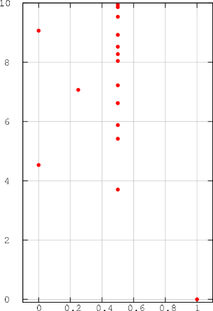
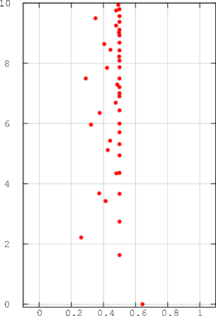
Figure 1. Zeros of the Selberg zeta-function $Z(\alpha,\cdot)=Z(\chi_{\alpha},\cdot)$ in the region $[0,1]\times i[0,10]$ of the spectral plane. On the left for $\alpha=0$, on the right for $\alpha=\frac{1}{10}$.

Via the Selberg trace formula, the zeros of function $Z(\Gamma,\chi;\cdot)$ are related to automorphic forms. This is the relation that we use in Sections LABEL:sect-prfs and LABEL:sect-spth for our theoretical approach.

We denote by $Z(\alpha,\beta)$ the Selberg zeta-function $\beta\mapsto Z\bigl{(}\Gamma_{0}(4),\chi_{\alpha};\beta)$ for $\alpha\in\mathbb{R}$. We consider its zeros in the region $\mathrm{Im}\,\beta>0$.

For each value of $\alpha\in\mathbb{R}$ the zeros of $Z(\alpha,\cdot)$ form a discrete set. In Figure 1 we give the non-trivial zeros of $Z(\alpha,\cdot)$ in the region $[0,1]\times i[0,10]$ in the $\beta$-plane for the trivial character, $\alpha=0$ (Table D.1 in [Fr]), and the nearby value $\alpha=\frac{1}{10}$ (interpolation of data discussed in §8.2 of [Fr]). In the unperturbed situation, $\alpha=0$, the zeros to the left of the central line, the resonances, are known to occur at the zeros of $\zeta(2\beta)$, of which only one falls within the bounds in the figure. There are also zeros at points $\frac{\pi i\ell}{\log 2}$ with $\ell\in\mathbb{Z}$.

We call zeros $\beta$ of $Z(\alpha,\cdot)=0$ with $\mathrm{Re}\,\beta=\frac{1}{2}$ eigenvalues, although we will see in §LABEL:sect-mf that $\beta-\beta^{2}$ qualifies better for that name. The lowest unperturbed eigenvalue is $.5+3.70331\,i$. Perturbation to $\alpha=\frac{1}{10}$ gives a more complicated set of zeros, many of which are eigenvalues.

In [Fr], §8.2, it is explained how zeros are followed as a function of the parameter. They follow curves that either stay on the central line, or move to the left of the central line and touch the central line only at some points.

1.1. Curves of eigenvalues

To exhibit curves of zeros of the Selberg zeta-function on the central line $\mathrm{Re}\,\beta=\frac{1}{2}$ we plot $\mathrm{Im}\,\beta$ as a function of $\alpha$.

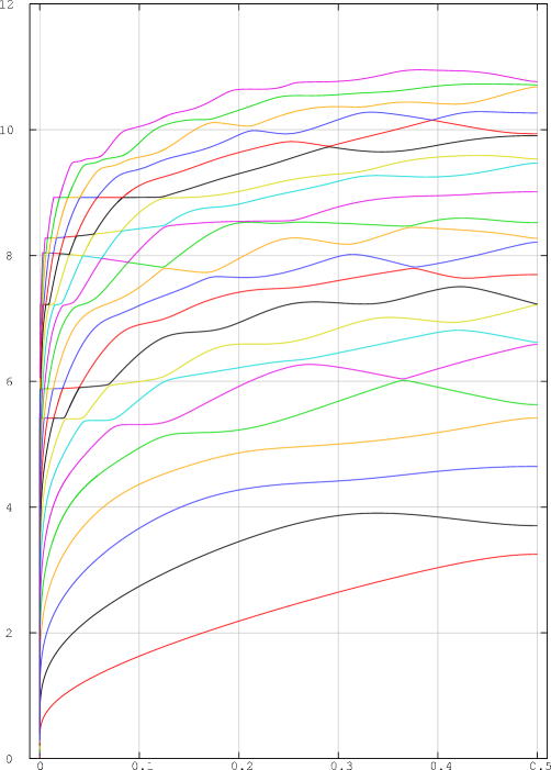
Figure 2. Zeros of $Z(\alpha,\beta)$ with $0<\alpha\leq\frac{1}{2}$, $\beta\in\frac{1}{2}+i(0,10)$. Horizontal: $\alpha$; vertical: $\mathrm{Im}\,\beta$.

The curves in Figure 2 were obtained in [Fr], by first determining for the arithmetical cases $\alpha\in\bigl{\{}\frac{1}{8},\frac{1}{4},\frac{3}{8},\frac{1}{2}\}$ all zeros in a region of the form $\frac{1}{2}+i[0,T]$. Here we display only those zeros which stay on the central line $\mathrm{Re}\,\beta=\frac{1}{2}$. The computations suggest that all these zeros go to $\beta=\frac{1}{2}$ as $\alpha\downarrow 0$, along curves that are almost vertical for small values of $\alpha$. Our first result confirms this impression, and makes it more precise:

Theorem 1.1.

For each integer $k\geq 1$ there are $\zeta_{k}\in(0,1]$ and a real-analytic map $\tau_{k}:(0,\zeta_{k})\rightarrow(0,\infty)$ such that $Z\bigl{(}\alpha,\frac{1}{2}+\nobreak i\tau_{k}(\alpha)\bigr{)}=0$ for all $\alpha\in(0,\zeta_{k})$.

For each $k\geq 1$

(1.3) $$\tau_{k}(\alpha)\;=\;\frac{\pi k}{-\log(\pi^{2}\alpha/4)}+{\mathrm{O}}\Bigl{(}\frac{k^{2}}{(\log\alpha)^{3}}\Bigr{)}\qquad\text{as }\alpha\downarrow 0\,.$$

So there are infinitely many curves of zeros going down as $\alpha\downarrow 0$, and for each curve the quantity $-\pi^{-1}\,\mathrm{Im}\,\beta\,\log\frac{\pi^{2}\alpha}{4}$ tends to an integer. Figure 3 shows that the computational data confirm the asymptotic behavior in (1.3).

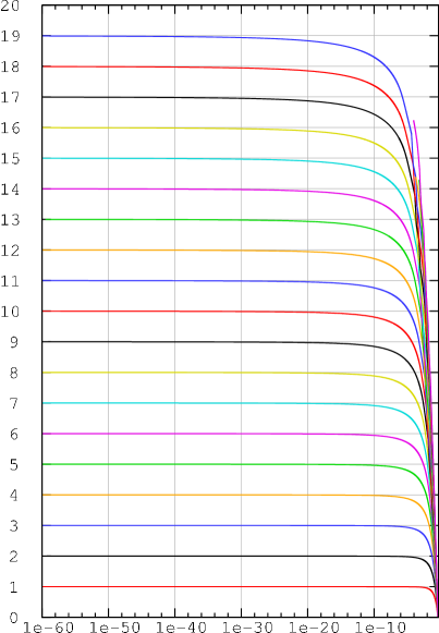
Figure 3. On the vertical axis the quantity $-\pi^{-1}\,\mathrm{Im}\,\beta\,\log\frac{\pi^{2}\alpha}{4}$ is given for those curves in the data set of [Fr] for which $\beta$ goes to $\frac{1}{2}$ along the central line as $\alpha\downarrow 0$. The horizontal axis gives $\alpha$ on a logarithmic scale. So $\alpha\downarrow 0$ means going to the left in the graph.

The theorem does not state that all zeros of the Selberg zeta-function on the central line occur in these families. The spectral theory of automorphic forms allows the possibility that there are other families.

Figure 2 shows also a regular behavior near many parts on the central line. By theoretical means we obtain:

Theorem 1.2.

Let $I\subset(0,\infty)$ be a bounded closed interval such that the interval $\frac{1}{2}+i\,I$ on the central line does not contain zeros of the unperturbed Selberg zeta-function $Z(0,\cdot)$.

Let for $t\geq 0$

(1.4) $$\varphi_{-}(t)\;=\;\arg\pi^{2it}\;\frac{2^{1+2it}-1}{2^{1-2it}-1}\;\frac{\zeta(-2it)}{\zeta(2it)}\,,$$

with $\zeta$ the Riemann zeta-function, be the continuous choice of the argument that takes the value $0$ for $t=0$.

For all sufficiently large $k\in\mathbb{Z}$ there is a function $a_{k}:I\rightarrow(0,1)$ inverting on $I$ the function $\tau_{k}$ of the previous theorem: $\tau_{k}\bigl{(}a_{k}(t))=t$ for $t\in I$. Uniformly for $t\in I$ we have

(1.5) $$a_{k}(t)\;=\;\pi^{-1}e^{\varphi_{-}(1/2+it)/2t+\pi k_{I}/2t}\,e^{-\pi k/t}\,\Bigl{(}1+{\mathrm{O}}\bigl{(}e^{-\pi k/t}\bigr{)}\Bigr{)}\qquad(k\rightarrow\infty)\,,$$

for some $k_{I}\in\mathbb{Z}$.

The theorem gives an assertion concerning the behavior of the zeros on the central line at given positive values $t$ of $\mathrm{Im}\,\beta$, and describes the asymptotic behavior as the parameter $k$ from the previous theorem tends to $\infty$. To compare this prediction with the data we determine by interpolation the value $a_{k}(t)$ for the curves used in Figure 3. The theorem predicts that

(1.6) $$\log\frac{a_{k}(t)}{\pi}+\frac{\pi k}{t}-\frac{\pi_{-}(1/2+it)}{2t}\,\approx\,\frac{\pi k_{I}}{2t}+{\mathrm{O}}\bigl{(}e^{-\pi k/t}\bigr{)}\,.$$

We used the data for the curves with $1\leq k\leq 19$ to compute an approximation of the quantity on the left in (1.6). We consider this as a vector in $\mathbb{R}^{19}$, with coordinates parametrized by $k$, and project it orthogonally on the line spanned by $(1,1,\ldots,1)$ with respect to the scalar product $(x,y)=\sum_{k=1}^{19}k^{20}\,x_{k}\,y_{k}$, and thus obtain approximations of $\pi k_{I}/2t$, which are given in Table 1.

$$\begin{array}[]{|c|ccccccccc|}\hline\cr t:&1&2&3&4&5&6&7&8&9\\ &-2.000&-2.000&-2.000&-2.000&-2.000&2.000&2.000&4.015&10.17\\ \hline\cr\end{array}$$

Table 1. Approximation of $k_{I}$ in (1.6).

Figure 4 illustrates the approximation of $k_{I}$ for more values of $t$ between $0.05$ and $9.00$.

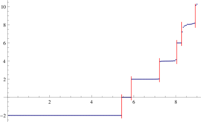
Figure 4. Approximation of $k_{I}$ for $t\in(0,9]\cap\frac{1}{20}\mathbb{Z}$. The vertical lines indicate the position of the unperturbed odd eigenvalues (from Table D.1 in [Fr]).

The intervals $I$ in the theorem should not contain zeros of the unperturbed Selberg zeta-function. Actually, the proofs will tell us that not all unperturbed zeros are not allowed to occur in $I$, only those associated to Maass cusp forms that are odd for the involution induced by $z\mapsto\bar{z}/(2\bar{z}-\nobreak 1)$. We have indicated the corresponding $t$-values by vertical lines in Figure 4.

1.1.1. Avoided crossings.

If one looks at the graphs of the functions $\tau_{k}$ in Figure 2 (ignoring the coloring) it seems that the graphs intersect each other. In the enlargement in Figure 5 most of these intersections turn out to be no intersections after all. This is the phenomenon of avoided crossings that is known to occur at other places as well; for instance in the computations of Strömberg in [Str].

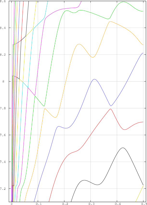
Figure 5. Enlargement of a subregion in Figure 2. Zeros of $Z(\alpha,\beta)$ with $0<\alpha\leq\frac{1}{2}$, $\beta\in\frac{1}{2}+i(7.1,8.6)$.

In the computations for [Fr] care was taken to decrease the step length whenever curves of zeros approached each other. In all cases this indicated that the curves of zeros do not intersect each other. Theoretically, we know that no intersections occur for the zeros moving along the central line in the region indicated in Lemma LABEL:lem-S-.

In Remark LABEL:rmk-av we will discuss that for some of the $t_{0}>0$ for which $Z(0,\frac{1}{2}+\nobreak it_{0})=0$ there may be a curve through $t_{0}$ in the $(\alpha,t)$-plane such that $\tau_{k}^{\prime}(\alpha)$ is relatively small for the value of $\alpha$ for which the graph of $\tau_{k}$ intersects the curve. We show this only under some simplifying assumptions formulated in Proposition LABEL:prop-av.

1.2. Curves of resonances

The zeros of $Z(\alpha,\beta)$ with $\beta$ to the left of the central line are more difficult to depict, since they form curves in the three-dimensional set of $(\alpha,\beta)$ with $\alpha\in(0,1)$ and $\beta\in\mathbb{C}$.

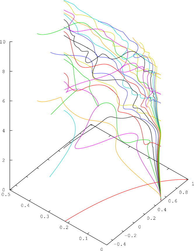
Figure 6. Zeros with $\mathrm{Re}\,\beta<\frac{1}{2}$, $\alpha>0$, in a $3$-dimensional graph. On the vertical axis $\mathrm{Im}\,\beta$ runs from $0$ to $10$. The ‘horizontal’ axis running to the left gives the coordinate $\alpha\in\bigl{(}0,\frac{1}{2}\bigr{)}$, and the ‘horizontal’ axis to the right gives $\mathrm{Re}\,\beta\in\bigl{(}-\frac{1}{2},1\bigr{)}$.

Figure 6 gives a three-dimensional picture. We see one curve in the horizontal plane, corresponding to $\mathrm{Im}\,\beta=0$. In this paper we do not consider real zeros of the Selberg zeta-function. Many curves originate for $\alpha\approx 0$ from $\beta=\frac{1}{2}$ and move upwards in the direction of increasing values of $\mathrm{Im}\,\beta$. On the right we see also a few more curves that wriggle up starting from higher values of $\mathrm{Im}\,\beta$.

In Figure 7

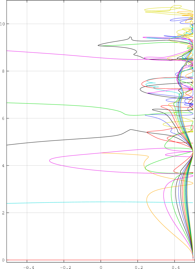
Figure 7. Curves of resonances in the complex plane. The vertical axis carries $\mathrm{Im}\,\beta$ and the horizontal one $\mathrm{Re}\,\beta$.

we project the curves onto the $\beta$-plane. In this projection we cannot see the $\alpha$-values along the curve. We see again the curves starting at $\beta=\frac{1}{2}$. Many of them seem to touch the central line at higher values of $\mathrm{Im}\,\beta$. The curves that start higher up are not well visible in this projection.

We can confirm certain aspects of these computational results by theoretical results. We start with the behavior of the resonances near $\bigl{(}0,\frac{1}{2}\bigr{)}$.

Theorem 1.3.

There are $\varepsilon_{1},\varepsilon_{2},\varepsilon_{3}>0$ such that all $(\alpha,\beta)$ that satisfy $Z(\alpha,\beta)=0$, $\alpha\in(0,\varepsilon_{1}]$, $\frac{1}{2}-\varepsilon_{2}\leq\mathrm{Re}\,\beta<\frac{1}{2}$, and $0<\mathrm{Im}\,\beta\leq\varepsilon_{3}$ occur on countably many curves

$$t\mapsto\bigl{(}\alpha_{k}(t),\sigma_{k}(t)+it\bigr{)}\qquad(0<t\leq\varepsilon_{3})\,,$$

parametrized by integers $k\geq 1$. The functions $\alpha_{k}$ and $\sigma_{k}$ are real-analytic. The values of $\sigma_{k}$ are in $\bigl{[}\frac{1}{2}-\nobreak\varepsilon_{2},\frac{1}{2}\bigr{)}$. For each $k\geq 1$ the map $\alpha_{k}$ is strictly increasing and has an inverse $t_{k}$ on some interval $(0,\zeta_{k}]\subset(0,\varepsilon_{1}]$. As $\alpha\downarrow 0$ we have

(1.7) $$t_{k}(\alpha) \;=\;\frac{\pi k}{|\log\pi^{2}\alpha|}+{\mathrm{O}}\Bigl{(}\frac{1}{|\log\pi^{2}\alpha|^{4}}\Bigr{)}\,,$$

(1.8) $$\sigma_{k}\bigl{(}t_{k}(\alpha)\bigr{)} \;=\;\frac{1}{2}-\frac{2(\pi k\log 2)^{2}}{|\log\pi^{2}\alpha|^{3}}+{\mathrm{O}}\Bigl{(}\frac{1}{|\log\pi^{2}\alpha|^{4}}\Bigr{)}\,.$$

The theorem confirms that there are many curves of resonances that approach the point $(0,\frac{1}{2})$ almost vertically as $\alpha\downarrow 0$. To check this graphically, one may consider the three quantities

(1.9) $$k_{1}(\alpha,\beta) \;=\;\sqrt{\bigl{(}\frac{1}{2}-\mathrm{Re}\,\beta\bigr{)}\,|\log\pi\alpha|^{3}/2\pi^{2}(\log 2)^{2}}\,,$$

$$k_{2}(\alpha,\beta) \;=\;\mathrm{Im}\,\beta\Bigl{(}\frac{\pi}{|\log\pi\alpha|}+\frac{\pi\,\log\pi}{|\log\pi\alpha|^{2}}+\frac{\pi(\log\pi)^{2}}{|\log\pi\alpha|^{3}}\Bigr{)}^{-1}\,,$$

$$k_{3}(\alpha,\beta) \;=\;\frac{2(\log 2)^{2}\,(\mathrm{Im}\,\beta)^{3}}{\pi\bigl{(}\frac{1}{2}-\mathrm{Re}\,\beta)}\,,$$

which should each approximate the “real” $k$ as $\alpha\downarrow 0$. Figure 8 illustrates $k_{3}$. Note that the horizontal scale gives $\alpha$ logarithmically, so the curves should tend to integers when going to the left. Although the data go down to $\alpha=10^{-60}$ the limit behavior is not clear in the picture.

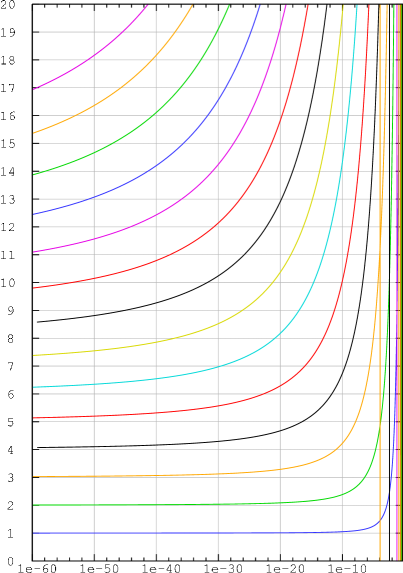
Figure 8. The quantity $k_{3}\bigl{(}\alpha,\beta\bigr{)}$ in (1.9) (vertical) as a function of $\alpha$ (horizontal) on a logarithmic scale, for several curves of resonances in [Fr].

In a non-graphical approach we approximate the limit value by finding the coefficients in a least square approximation

(1.10) $$k_{j}(\alpha,\beta)\;\approx\;\sum_{\ell=1}^{5}\frac{c_{\ell}}{|\log\alpha|^{\ell}}$$

over the $500$ data points with lowest values of $\alpha$ on each of the curves of resonances going to $\bigl{(}0,\frac{1}{2}\bigr{)}$. The coefficient $c_{0}$ should be an approximation of the limit. The data are in Table 2.

file name	$k_{R,1}$	$k_{R,2}$	$k_{R,3}$
S6	1.00000077911	1.00000012847	0.999999581376
S8	1.99993359598	2.00000692659	2.00002268168
S7	2.99969624243	2.99999718822	3.00014897712
S1-1	3.98453704088	3.99972992678	4.00794474117
S3	4.97680447599	4.99941105921	5.01294455984
S16	5.9998899911	5.99996250451	6.00002349805
S19	6.96419831285	6.99744783611	7.03093500105
S23	8.09149912519	7.9904003854	8.02661700448
S26	9.03588236648	8.99230468926	9.04177665474
S11	10.1247216267	9.99015681093	10.0254416847
S34	11.4775951755	10.9860223595	10.9219590835
S43	11.93647544	11.9959050481	12.0661799032
S38	13.3059450769	12.9885322374	12.9785198908
S46	14.0371581712	13.9931918442	14.0160494173

Table 2. Least square approximation of the limits $k_{R,j}$ of the quantities $k_{j}$ in (1.9). (The first column refers to the naming in [Fr] of the curves of zeros.)

This gives a reasonable confirmation that (1.7) and (1.8) describe the asymptotic behavior of the data. We also experimented with direct least square approximation of the coefficients of the expansion of $t_{k}(\alpha)$ and $\sigma_{k}\bigl{(}t_{k}(\alpha)\bigr{)}$ as a function of $\frac{1}{|\log\pi^{2}\alpha|}$. The results from the approximation of $\sigma_{k}\bigl{(}t_{k}(\alpha)\bigr{)}$ were less convincing than those in Table 2.

The next result concerns curves higher up in the $\beta$-plane.

Theorem 1.4.

Let $I$ be a bounded interval in $(0,\infty)$ such that $\{0\}\times\left(\frac{1}{2}+iI\right)$ does not contain zeros of the unperturbed Selberg zeta-function $Z(0,\cdot)$.

There are countably many real-analytic curves of resonances of the form

$$t\mapsto\bigl{(}\alpha_{k}(t),\sigma_{k}(t)+it\bigr{)}\qquad\text{ with }t\in I\,,$$

parametrized by integers $k\geq k_{1}$ for some integer $k_{1}$. Uniformly for $t\in I$ we have the relations

(1.11) $$\alpha_{k}(t) \;=\;\frac{1}{\pi}\,e^{A(1/2+it)/2t}\,e^{-\pi k/t}\,\Bigl{(}1+{\mathrm{O}}\bigl{(}\frac{1}{k}\bigr{)}\Bigr{)}\,,$$

(1.12) $$\frac{1}{2}-\sigma_{k}(t) \;=\;\frac{t}{2\pi k}\,M\bigl{(}\frac{1}{2}+it)+{\mathrm{O}}\Bigl{(}\frac{1}{k^{2}}\Bigr{)}\,,$$

as $k\rightarrow\infty$, where $M(t)$ and $A(t)$ are the real and imaginary part of a continuous choice of

$$\log\Bigl{(}\pi^{2it}\,\bigl{(}2^{1+2it}-1\bigr{)}\,\frac{\zeta(-2it)}{\zeta(2it)}\Bigr{)}\,.$$

If we would use a standard choice of the argument the function $A$ would have discontinuities. The parameter $k$ is determined by the choice of the branch of the logarithm. The theory does not provide us, as far as we see, a way to relate the numbering of the branches for different intervals $I$.

We compare relation (1.11) with the data files in the same way as we used for Theorem 1.4. The theorem says that the relation holds for some choice $A$ of the argument. We picked a continuous choice. Then we expect a factor $e^{\pi k_{I}/t}$ in (1.11) with $k_{I}$ constant on intervals as indicated in the theorem. This leads to Figure 9.

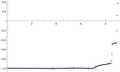
Figure 9. Approximation of $k_{I}$ for $t\in(0,9]\cap\frac{1}{20}\mathbb{Z}$. The vertical lines indicate the position of unperturbed even eigenvalues (from Table D.1 in [Fr]).

The function $M$ in (1.12) has the simple form $M(t)=\log\bigl{|}2^{1+2it}-\nobreak 1\bigr{|}$. Figure 10 gives this function and the approximation of it based on (1.12).

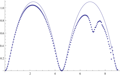
Figure 10. The function $t\mapsto\log\bigl{|}2^{1+2it}-\nobreak 1\bigr{|}$ and its approximation based on (1.12).

Figures 9 and 10 show differences that we do not understand well.

In Figure 7 it seems that at $\beta\approx\frac{1}{2}+4.5\,i$ many curves touch the central line. Moreover, relation (1.12) suggests that there are infinitely many curves that are tangent to the central line at the points $\frac{1}{2}+\frac{\pi i}{\log 2}\ell$ with $\ell\in\mathbb{Z}$. In Figure 7 there seems to be a common touching to the central line at $\beta\approx\frac{1}{2}+9.0\,i$ as well. Figure 11 gives a closer few at the resonances near $\beta=\frac{1}{2}+\frac{\pi i}{\log 2}$ for curves computed in [Fr].

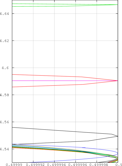
Figure 11. Enlargement of part of Figure 7 near $\beta=\frac{1}{2}+\frac{\pi i}{\log 2}$.

There is no common touching point, but a sequence of tangent points approaching $\frac{1}{2}+\frac{\pi i}{\log 2}$. Conclusions 8.2.32 and 8.2.33 in [Fr] give a further discussion. Concerning this phenomenon we have the following result:

Theorem 1.5.

Suppose that an interval $I$ as in Theorem 1.4 contains in its interior a point $t_{\ell}:=\frac{\pi\ell}{\log 2}$ with an integer $\ell\geq 1$. Then there is $k_{2}\geq k_{1}$ such that for each $k\geq k_{2}$ the curve $t\mapsto\sigma_{k}(t)+\nobreak it$ in Theorem 1.4 is tangent to the central line in a point $\frac{1}{2}+it_{\ell}+i\delta_{k}\in\frac{1}{2}+iI$, and the $\delta_{k}$ satisfy

(1.13) $$\delta_{k}\;=\;\frac{\eta_{2}}{\pi^{2}}e^{A(1/2+it_{\ell})/t_{\ell}}\,e^{-2\pi k/t_{\ell}}\,\Bigl{(}1+{\mathrm{O}}\bigl{(}k^{-1}\bigr{)}\Bigr{)}\,,$$

for some $\eta_{2}\in\mathbb{R}$. The function $A$ is as in Theorem 1.4.

We do not get information concerning $\eta_{2}$ from the theory. Table 8.8 in [Fr] gives approximated tangent points near $\frac{1}{2}+\frac{\pi i}{\log 2}$. In Figure 12 we give the corresponding approximations of $\log\eta_{2}$.

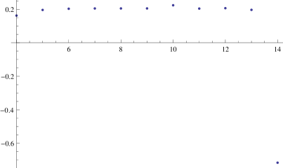
Figure 12. Approximation of $\eta_{2}$ in Theorem 1.5 for $\ell=1$, based on Table 8.8 in [Fr].

Remark 1.6.

Theorems 1.1–1.5 have been motivated by part of the observations of Fraczek. In the next sections we present proofs that do not depend on the computations. The comparisons of the theoretically obtained asymptotic results with the computational data is in some cases convincing, and show in other cases discrepancies that we do not understand fully.