Critical fields and growth rates of the Tayler instability as probed by a columnar gallium experiment

Abstract

Many astrophysical phenomena (such as the slow rotation of neutron stars or the rigid rotation of the solar core) can be explained by the action of the Tayler instability of toroidal magnetic fields in the radiative zones of stars. In order to place the theory of this instability on a safe fundament it has been realized in a laboratory experiment measuring the critical field strength, the growth rates as well as the shape of the supercritical modes. A strong electrical current flows through a liquid-metal confined in a resting columnar container with an insulating outer cylinder. As the very small magnetic Prandtl number of the gallium-indium-tin alloy does not influence the critical Hartmann number of the field amplitudes, the electric currents for marginal instability can also be computed with direct numerical simulations. The results of this theoretical concept are confirmed by the experiment. Also the predicted growth rates of the order of minutes for the nonaxisymmetric perturbations are certified by the measurements. That they do not directly depend on the size of the experiment is shown as a consequence of the weakness of the applied fields and the absence of rotation.

1 Introduction

Sufficiently strong, not current-free toroidal magnetic fields become unstable due to the non-axisymmetric Tayler instability (“TI”; Tayler 1957, 1960, Vandakurov 1972, Tayler 1973). The necessary energy is provided by the electric current, hence the instability also exists without plasma motion, e.g. due to stellar rotation. So far, mostly astrophysics-related numerical simulations of the TI are very rare (Braithwaite & Spruit 2004, Braithwaite 2006, Gellert et al. 2008, Moll et al. 2008).

The existence of the magnetic Tayler instability likely has immense astrophysical consequences. Ott et al. (2006) concluded from their supernova core-collapse simulations (with the rotation of the initial iron core as the free parameter) that the rotation period of a newly born neutron star should not exceed 1 ms, in contrast to the observations that peak with periods around 10–100 ms. Berger et al. (2005) argue for an upper limit of 10 km/s rotation velocity for white dwarfs using their spectroscopy of the rotational broadening of the Ca ii K line. Neutron stars as well as white dwarfs are compact remnants of stellar cores that exhibit a specific angular momentum of $10^{13\dots 14}$ cm²/s. However, for their progenitors, Berger et al.’s simulations provide values of more than 10¹⁶ cm²/s, indicating two missing orders of magnitude between the hydrodynamic theory and the observations. Suijs et al. (2008) indeed show that an evolution scenario for stars with 1–3 M_☉ that includes small-scale Maxwell stresses can explain the extreme spin down of the stellar core by typically two orders of magnitude.

Furthermore, we know from helioseismology that the solar radiative core rotates basically rigidly despite that the microscopic viscosity of the solar plasma yields a diffusion time much longer than the Sun’s lifetime. One would need an effective viscosity of about $10^{5}$ cm²/s to explain the decay of an initial rotation law within the lifetime of the Sun. It is thus tempting to probe whether an instability-driven angular momentum transport – either due to magnetic instabilities of fossil fields and/or of induced internal toroidal fields – is strong enough to produce an increase of the microscopic viscosity in the radiative zone by several orders of magnitude (Eggenberger et al. 2005). For example, one finds for the upper part of the solar radiative core about 600 Gauss as the minimum amplitude of a toroidal field to become unstable.

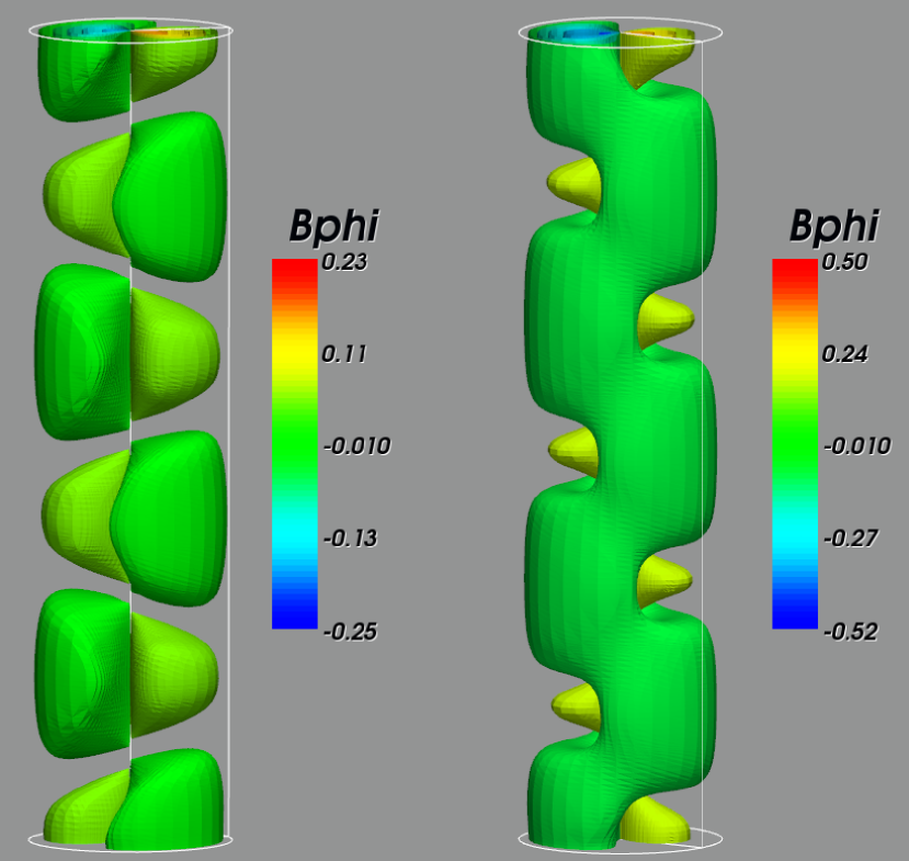
Figure 1: Isosurface plot of the magnetic field perturbation $b_{\phi}$ for a magnetic Prandtl number ${\rm Pm}=0.01$ (left) and ${\rm Pm}=1$ (right). The direct numerical simulation was carried out with an insulating outer cylinder, $R_{\rm in}=0$, a Hartmann number $\rm Ha=30$, and perfect-conducting endplates. Note the rather high amplitudes of the perturbation patterns (normalized with the outer azimuthal background field, not shown).

The lithium at the surface of cool main-sequence stars depletes with a timescale of $\approx$1 Gyr. Lithium is burned at temperatures in excess of $2.6\cdot 10^{6}$ K that, in case of today’s Sun, exist about 40,000 km below the base of the convection zone. Consequently, there must be a diffusion process between the upper layers and the regions of the burning temperature. Its time scale must be one or two orders of magnitude shorter than the molecular diffusion in order to explain the above lithium decay time. On the other hand, any enhanced chemical mixing comes along with an intensified mixing of the angular momentum. Considering transport processes in the radiative interior of massive (15 M_⊙) main-sequence stars, Spruit (2002) and Maeder & Meynet (2003, 2005) computed viscosities up to $10^{13}$ cm²/s for an equatorial rotational velocity of 300 km/s with which the internal stellar rotation becomes rigid after a few thousand years. Heger et al. (2005) and Woosley & Heger (2006) followed on this basis the rotational history of massive main-sequence stars until their collapse-end.

Rotationally induced mixing is also included in the stellar evolution codes by Heger & Langer (2000), and Yoon et al. (2006) presented evolutionary models of rotating stars with different metalicity. As even the lifetime and thus the evolutionary path in the H-R diagram is influenced by the mixing, the action of magnetic instabilities must also influence the ages of young stellar clusters. This may alter the rotation-activity-age relation for low-mass stars which very much depends on the age determination of young clusters (Barnes 2010). Brott et al. (2008) demonstrate that the magnetic-induced chemical mixing in massive stars must even be reduced to avoid conflicts with the observations.

A dynamo action on the basis of TI, as proposed by Spruit (1999, 2002) and Braithwaite (2006), could not be confirmed so far (Zahn et al. 2007). The suggestion is that differential rotation and a magnetic kink-type instability could jointly drive a dynamo in stellar radiative zones. If existent, such a dynamo would also be effective for the angular momentum transport and the chemical mixing in stellar interiors. However, more detailed numerical models are needed to investigate the dynamo efficiency of the TI, e.g. by computing the magnetic-induced (magnetic) dissipation and the possible existence of the predicted kind of $\alpha$-effect.

In general, the search for the possible existence of kinetic/magnetic helicity and/or $\alpha$-effect leads to the investigation of the stability of background fields with finite current helicity $\mbox{\boldmath$B$}\cdot{\rm curl}\ \mbox{\boldmath$B$}$. Such a field geometry results by a combination of axial currents with axial fields. The reason is that the TI of an purely azimuthal field does not produce an instability pattern with finite helicity so that such simple fields would not produce any TI-induced $\alpha$-effect. The rotation of the container only plays here a minor role but spontaneous parity breaking bifurcations of solutions with an equal mixture of both signs of helicity in MHD system which might be unstable, is now under discussion (Chatterjee et al. 2011, Bonanno et al. 2012).

This situation is drastically changed if an axial field is added to the current-induced azimuthal field. Small-scale kinetic and current helicities immediately result which are anticorrelated to the current helicity of the background field. The corresponding $\alpha$-effect is highly anisotropic ($\alpha_{\phi\phi}\cdot\alpha_{zz}<0$) where the $\alpha_{\phi\phi}$ has the same sign as the current helicity of the background field (Gellert et al. 2011). On the other hand, it is clear that the combination of axial currents and axial fields may drastically change the excitation conditions. Bonanno & Urpin (2008) found a stabilization of axisymmetric TI modes for finite axial fields. Also the nonaxisymmetric modes are stabilized for fields with large pitch angle $|B_{z}/B_{\phi}|$ while the fastest growing modes always possess higher azimuthal wave numbers (Bonanno & Urpin 2011, Rüdiger et al. 2011b).

To our knowledge, the pure form of the TI, i.e. its action in an incompressible fluid (Tayler 1960), was unknown in experimental physics so far (see also Meynet & Maeder 2005). This is in contrast to the comprehensive experience in plasma physics where the compressible counterpart of the TI is better known as the kink instability ($m=\pm 1$) in a z-pinch, i.e. the limit of the Kruskal-Shafranov instability when the safety factor goes to zero (Bergerson et al. 2006). In order to place the many magnetic numerical simulations in stellar physics onto a safe fundament, we conducted and present here the first successful realization of the TI in an experiment with an incompressible fluid. The critical magnetic field strength and the supercritical growth rates are calculated both quasi-analytically and by numerical simulations and are compared with the onset of the instability in the columnar “gallium Tayler instability experiment”, dubbed GATE. The design and the technical details of the experiment are given by Seilmayer et al. (2012).

2 Theory and simulations

A cylindrical Taylor-Couette container is considered confining a toroidal magnetic field of given amplitude. The container possesses an inner and an outer cylinder with radii $R_{\rm in}$ and $R_{\rm out}$ with $r_{\rm in}={R_{\rm{in}}}/{R_{\rm{out}}}$. The radius of the inner cylinder is assumed as very small including the limit zero. The fluid between the cylinders is assumed to be incompressible with uniform density and dissipative with both the kinematic viscosity $\nu$ and the magnetic diffusivity $\eta$.

The solution of the stationary induction equation inside the outer cylinder under the presence of a uniform electric current $I$ reads

$$B_{\phi}=\frac{I}{5R^{2}_{\rm out}}R$$ (1)

(see Roberts 1956; Pitts & Tayler 1985; Spies 1988). Rüdiger & Schultz (2010) have shown for all azimuthal Fourier modes that for resting cylinders the critical value of the Hartmann number

$${\rm Ha}=\frac{B_{\rm out}R_{\rm out}}{\sqrt{\mu_{0}\rho\nu\eta}}.$$ (2)

does not depend on the magnetic Prandtl number $\rm Pm=\nu/\eta$. It is thus allowed for the calculation of the critical Hartmann number to solve the complete set of equations only for the numerically most simple case of $\rm Pm=1$. This is not true, however, with respect to the growth rates.

If the radial profiles of the azimuthal field are not too steep the current-driven TI is mainly a non-axisymmetric instability. While for the stability of non-axisymmetric modes the necessary and sufficient condition is

$$\frac{{\rm{d}}}{{\rm{d}}R}(RB_{\phi}^{2})<0$$ (3)

(Tayler 1973), the same reads for axisymmetric modes as

$$\frac{{\rm{d}}}{{\rm{d}}R}\left(\frac{B_{\phi}}{R}\right)^{2}<0$$ (4)

(Velikhov 1959, Chandrasekhar 1961). The stable domain for axisymmetric modes thus always includes the profile $B_{\phi}\propto R$ noted in Eq. (1) which after Eq. (3) will be unstable against non-axisymmetric perturbations. In this case both the modes with $+m$ and $-m$ are simultaneously excited so that the resulting field and flow components do not perform any azimuthal drift. The most unstable mode is $|m|=1$. Figure 1 shows an isosurface plot of the nonaxisymmetric field pattern of the dynamic azimuthal component $b_{\phi}$ from nonlinear simulations for both $\rm Pm=0.01$ and $\rm Pm=1$. The field is normalized with the fixed outer value of the applied toroidal field. One finds a maximum perturbation amplitude of around 50% of the applied field for $\rm Pm=1$. This surprisingly high value varies only weakly with $\rm Pm$: it only varies by a factor of two if $\rm Pm$ varies by two orders of magnitude. The wave number is also nearly constant.

The nonlinear MHD code of Gellert et al. (2007) can be used to compute the critical Hartmann number for $\rm Pm=1$, which then holds for all $\rm Pm$. A first calculation concerns an infinite cylinder with insulating walls while a second one concerns a closed cylinder with perfect-conducting endplates. The resulting instability conditions are ${\rm Ha}\simeq 22.3$ for the infinite container and ${\rm Ha}\simeq 22.5$ for the closed container. As expected for closed containers the TI is slightly stabilized by the endplates because of the wave number restrictions.

The Hartmann number (Eq. 2) determines the electrical current via

$$I=5{\rm Ha}\sqrt{\mu_{0}\rho\nu\eta},$$ (5)

where for the material constant of the used gallium-indium-tin alloy one finds $\sqrt{\mu_{0}\rho\nu\eta}=25.3$ in c.g.s. for a temperature of 300 K ($\rho=6.44$ g/cm³, $\eta=2440$ cm²/s and $\nu=3.25\cdot 10^{-3}$ cm²/s). With these numbers the minimum electric current for excitation of TI becomes 2.8 kA. This is a minimum value which cannot be optimized by variation of the radial size of the container.

3 The linearized system of equations

Sofar the magnetic Prandtl number does not play any role. However, this is not true for both the growth rates and also the wave numbers of the unstable modes for supercritical magnetic fields. Because of the low magnetic Prandtl number for liquid metals they can accurately be computed only with a linear code. The linearized MHD equations for the flow and field perturbations in a conducting fluid subject to a magnetic background field $B$ are

$$\frac{\partial\mbox{\boldmath$u$}}{\partial t}=-\nabla(p/\rho)+$$

$$\quad\quad\quad+\nu\Delta\mbox{\boldmath$u$}+{\rm curl}{\mbox{\boldmath$B$}}\times\mbox{\boldmath$b$}+{\rm curl}\mbox{\boldmath$b$}\times{\mbox{\boldmath$B$},}$$

$$\frac{\partial\mbox{\boldmath$b$}}{\partial t}=\eta\Delta\mbox{\boldmath$b$}+{\rm curl}\big{(}\mbox{\boldmath$u$}\times{\mbox{\boldmath$B$}}\big{)}$$ (6)

with ${\rm div}\ {\mbox{\boldmath$u$}}={\rm div}\ {\mbox{\boldmath$b$}}=0$ and $p$ the pressure fluctuations. The boundary conditions for the flow are always no-slip and the outer cylinder is always assumed to be insulating. For the space within the inner cylinder, two magnetic conditions are possible: a vacuum or a perfect conductor. None of them exactly fits in the limit $R_{\rm in}\to 0$ to the regularity conditions at the axis which for $m=1$ reads ${\rm d}b_{R}/{\rm d}R={\rm d}b_{\phi}/{\rm d}R=b_{z}=0$. These different boundary conditions are applied at $R_{\rm{in}}$. In a series of calculations the limit $R_{\rm{in}}\to 0$ is approached. We found highly convergent solutions for the inner perfect-conductor solutions while the vacuum condition creates severe numerical problems for $r_{\rm in}\to 0$.

The wave number is varied as long as the corresponding Hartmann number takes its minimum. A vanishing growth rate provides the critical Hartmann number or, using Eq. (5), the critical electric current of the TI. Figure 2 provides the behavior of $\rm Ha$ for $R_{\rm in}\to 0$. In this case one finds that $\rm Ha$ is almost independent of $r_{\rm in}$ but for intermediate values $\rm Ha$ increases. For very small $R_{\rm in}$ the result is $\rm Ha=22$. The critical strength of the electric current is thus 2.78 kA, corresponding to Eq. (1) to an outer azimuthal field of about 110 Gauss. Evidently, the above results of the nonlinear simulations for ${\rm Pm}=1$ and the limit of the linear calculations for $R_{\rm in}\to 0$ with ${\rm Pm}=10^{-6}$ indeed coincide.

In a resting container and a fluid with magnetic Prandtl number of order unity one has only two frequencies: the diffusion frequency $\omega_{\eta}=\eta/R_{\rm out}^{2}$ and the Alfvén frequency $\Omega_{\rm A}=B_{\phi}/\sqrt{\mu_{0}\rho R^{2}_{\rm out}}$ of the toroidal field. Its ratio defines the limit of low-conductivity (or weak-field, $\omega_{\eta}\gg\Omega_{\rm A}$) and high-conductivity (or strong-field, $\omega_{\eta}\ll\Omega_{\rm A}$). Hence, the growth rate of the instability must be a linear function of these two frequencies in form of $\Omega_{\rm A}$ and $(\Omega_{\rm A}/\omega_{\eta})\Omega_{\rm A}$. It is also clear that in the high-conductivity limit only the term linear in $\Omega_{\rm A}$ can appear. In the low-conductivity limit the form quadratical in $\Omega_{\rm A}$, i.e.

$$\omega_{\rm gr}=\Gamma\frac{B^{2}_{\rm out}}{\mu_{0}\rho\eta},$$ (7)

may dominate where the factor $\Gamma$ for wide gaps varies only by a factor of four when the magnetic Prandtl number varies by four orders of magnitude (Rüdiger et al. 2011a). Note that in the low-conductivity limit the radial scale does not occur in Eq. (7). For highly supercritical Hartmann numbers Eq. (7) smoothly changes to the linear relation $\omega_{\rm gr}\propto\Omega_{\rm A}$ which does no longer depend on the microscopic diffusivities but which strongly decreases for increasing radius. The transition to the linear relation requires the higher Hartmann numbers the smaller the magnetic Prandtl number is. To date the transition can only be seen numerically, not experimentally.

Figure 2: Numerical values of the critical Hartmann number ${\rm Ha}$ for large gaps ($r_{\rm in}\ll 1$) between (infinitely) long cylinders. The outer boundary condition is vacuum, within the inner cylinder is vacuum or a perfectly conducting material. The curves are valid for all $\rm Pm$.

For $\rm Pm\simeq 10^{-(5\dots 6)}$ the calculation of the growth rates leads to $\Gamma\simeq 0.04$. The high value of the magnetic diffusivity of the fluid conductor leads to growth times of about 300 s for supercritical electric currents of order 4 kA (Fig. 4). These time scales are so long that a secondary circulation may arise in the experiment due to the internal Joule heating of the fluid. In the linear theory there is no magnetic stabilization mechanism as, e.g., it exists for strong fields for the magnetorotational instability (Balbus & Hawley 1991).

The optimized wave numbers prove to be nearly independent of the magnetic field and the geometry of the container (Fig. 3). They describe the axial scale $\delta z$ of the instability pattern after the relation

$$\frac{\delta z}{R_{\rm out}-R_{\rm in}}=\frac{\pi}{k},$$ (8)

so that $k\simeq\pi$ describes a circular cell pattern. As always $k<\pi$ the cells prove to be slightly elongated in axial direction. Moreover, the elongation does not depend on the magnetic field amplitude and the size of the gap. Even slow rotation has a very weak influence with the expected tendency to make the cells more flat.

Figure 3: The optimized wave numbers for two values of the radius of the inner cylinder ($r_{\rm in}=0.05$, $r_{\rm in}=0.12$) with perfect-conductor conditions at both boundaries without (dashed) and with rotation of Reynolds numbers 500, 1000 and 2000. The dotted line gives the wave number for circular-shaped cells after (8). The cells are thus elongated in the axial direction by only 8%. $\rm Pm=10^{-6}$.

4 The experimental results

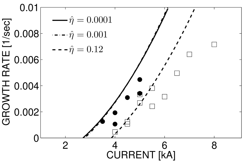
Figure 4: Observed and calculated growth rates in the columnar container with wide gaps: i) inner cylinder with 1.2 cm diameter ($r_{\rm in}=0.12$, open squares; dashed line) and ii) no inner cylinder (full circles, solid line). In the numerical simulations the inner cylinder is considered as vacuum (dashed line) or as perfect conductor (both left lines). For very small $r_{\rm in}$ the growth rates are independent of $r_{\rm in}$ (dot-dashed line: $r_{\rm in}=0.001$, solid line: $r_{\rm in}=0.0001$).

The experimental apparatus consists of an insulating cylinder with a height of 75 cm and a radius $R_{\rm out}$ of 5 cm which is filled with the eutectic alloy GaInSn. An inner cylinder with radius $R_{\rm in}$ of 0.6 cm can be inserted. At the top and bottom, the liquid column is in contact with two massive copper electrodes which are connected by water cooled copper tubes to an electric power supply. This power supply is able to provide up to 8 kA of current. Although for later experiments the use of Ultrasonic Doppler Velocimetry (UDV) for the measurement of the axial velocity perturbation is envisioned, for the first experiment it has been decided not to use any inserts that could disturb the homogeneous current from the copper electrodes to the liquid. With 14 fluxgate sensors the modifications of the magnetic fields that result from the TI are detected. Eleven of these sensors are positioned along the vertical axis, while the remaining three are positioned along the azimuth in the upper part. Such measurements give the geometry of the field, thus its shape in azimuthal and axial direction as well as the minimum current to excite the TI (Seilmayer et al. 2012).

In all cases of instability the observed pattern of the magnetic perturbations is a nonaxisymmetric one with $m=1$. Figure 4 shows the experimental results for the growth rates in comparison with the theoretical calculations for containers with very wide gaps between the cylinders. The theoretical result does not depend on $r_{\rm in}$ for $r_{\rm in}\ll 1$ so that these results may serve as a good proxy for the experiment without any inner cylinder (red asterisks in Fig. 4). For comparison, the data sets of a second experiment with an inner insulating cylinder with $r_{\rm in}=0.12$ (green squares in Fig. 4) are given. As expected this experiment requires clearly stronger electrical currents to excite TI compared to the experiment without an inner cylinder.

For low growth rates the experimental data fit the theoretical curves quite well. The agreement is almost perfect for the container with $r_{\rm in}=0.12$. For this case one finds a relation $\omega_{\rm gr}\simeq\gamma(I^{2}-I_{\rm crit}^{2})$ with $\gamma=2.7\cdot 10^{-10}$ so that after Eq. (1) a value of $\Gamma\simeq 0.038$ results in perfect agreement with the theory. The theory, however, always provides the maximum growth rates optimized with the wave number. The observed growth rates should thus never lie above the theoretical values which indeed is the case (except one single square).

5 Discussion

Motivated by its astrophysical relevance the Tayler instability has been probed by an experiment which showed not only its fundamental existence but also many specific details. To avoid the suppressing action of rotation a resting fluid conductor for the electric current has been used. We have shown that the Tayler instability in the experiment appears at the predicted Hartmann numbers. As expected, the azimuthal Fourier mode with $m=1$ dominates the unstable magnetic pattern. Also confirmed is the theoretical result that the critical Hartmann number for nonrotating fluids does not depend on the magnetic Prandtl number. Finally, the validity of relation (7) for the growth rate is shown for very small magnetic Prandtl numbers, which has previously been derived with a linear theory. This relation holds in the low-conductivity limit $\omega_{\eta}\ll\Omega_{\rm A}$ while for high conductivity the growth rate becomes linear in $\Omega_{\rm A}$. The experiment presented here validates the lower quadratic part of the growth rate curve; the transition shown in Fig. 5 towards the linear relation for high-conductivity, which is characteristic for astrophysical applications, requires larger Hartmann numbers, thus stronger currents.

For slightly supercritical Hartmann numbers the measured growth rates are in near perfect agreement with the theoretical values. For higher Hartmann numbers, however, they lie somewhat below the theoretical values. A stabilization effect evidently exists and is more effective for higher amplitudes of the electrical current than for lower values. A natural explanation of this phenomenon could be the generation of axial field components by nonaxisymmetric axial flows. Test calculations have shown that indeed even a nonaxisymmetric axial field pattern would reproduce the observed reduction of the growth rates for supercritical electric currents. Another possible explanation, at least of parts of this effect, is suggested by Eq. (7) as an amplification of the magnetic diffusivity $\eta$ during the experiment. This can be due to the internal heating of the fluid conductor which leads to higher $\eta$ via its temperature dependence (about 10% by increase of the temperature of 75 K). The counteracting density reduction is much weaker. The data in Fig. 4 do not exclude this possibility. For its final confirmation further measurements for stronger currents are necessary.

Another dynamical stabilization may follow from the production of an extra turbulence diffusivity $\eta_{\rm T}$ by the TI itself. By numerical simulations we have shown that the maximal value of the ratio $\eta_{\rm T}/\eta$ is only of order unity (Gellert & Rüdiger 2009) which could also be consistent with the presented data. Further experiments with special container constructions to reduce the internal heating must show whether the stabilization shown in Fig. 4 is due to the possible axial field component or also due to temperature-effects and dynamical influences.

Figure 5: The normalized growth rate of TI in a container with $r_{\rm in}=0.05$ without rotation (dashed) and with rotation of Reynolds numbers 500, 1000 and 2000. The reference frequency is $\sqrt{\nu\eta}/R^{2}_{\rm out}$. Note the suppression of the instability by the global rotation.

That the radial scale does not appear in the growth rate (7) is an exception. It changes for strong fields ($\omega_{\rm gr}\propto\Omega_{\rm A}$) as well as for weak fields when taking into account the (suppressing) influence of a given basic rotation. Then growth rates also depend on the radial scale. For slow rotation the growth rate (7) then formally must be divided by the magnetic Reynolds number of this rotation so that $\omega_{\rm gr}\propto\Omega_{\rm A}^{2}/\Omega$ results. The calculations show that this rotation-modified theoretical form of the growth rate of the TI can also be probed experimentally. For strong enough magnetic fields, however, the rotation does no longer influence the linear relation between $\omega_{\rm gr}$ and $\Omega_{\rm A}$ . Thus experiments with resting containers only slightly overestimate the characteristic growth rates, if the rotation is not too fast (Fig. 5).

It is obvious that the experiment possesses a great potential for studies about the TI-induced eddy diffusivities and – if the background field is modified by axial field components to helical structures – about the formation and evolution of small-scale kinetic and magnetic helicities and even the $\alpha$-effect.

References

- Balbus & Hawley (1991) Balbus, S. A. & Hawley, J. F. 1991, ApJ, 376, 214
- (2) Barnes, S. A. 2010, ApJ, 722, 222
- (3) Berger, L., Koester, D., Napiwotzki, R., Reid, I. N., & Zuckerman, B. 2005, A&A, 444, 565
- (4) Bergerson, W. F. et al. 2006, Phys. Rev. Lett., 96, 015004
- (5) Bonanno, A., & Urpin, V. 2008, A&A, 488, 1
- (6) Bonanno, A., & Urpin, V. 2011, A&A, 525, A100
- (7) Bonanno, A., Brandenburg, A., Del Sordo, F. & Mitra, D., 2012, arXiv: astro-ph/1204.0081
- (8) Brott, I., Hunter, I., Anders, P., & Langer, N. 2008, in AIP Conf. 990, First Stars III, eds. B.W. O’Shea et al., 273
- (9) Braithwaite, J. 2006, A&A, 449, 451
- (10) Braithwaite, J., & Spruit, H. C. 2004, Nature, 431, 819
- (11) Chandrasekhar, S. 1961, Hydrodynamic and hydromagnetic stability (Oxford: Clarendon)
- (12) Chatterjee, P., Mitra, D., Brandenburg, A. & Rheinhardt, M. 2011, PRE, 84, 5403
- (13) Eggenberger, P., Maeder, A., & Meynet, G. 2005, A&A, 440, L9
- (14) Gellert, M., Rüdiger, G., & Fournier, A. 2007, Astron. Nachr., 328, 1162
- (15) Gellert, M., Rüdiger, G., & Elstner, D. 2008, A&A, 489, L33
- (16) Gellert, M., & Rüdiger, G. 2009, PRE, 80, 46314
- (17) Heger, A., & Langer, N. 2000, ApJ, 544, 1016
- (18) Heger, A., Woosley, S. E., & Spruit, H. C. 2005, ApJ, 626, 350
- (19) Maeder, A., & Meynet, G. 2003, A&A, 411, 543
- (20) Maeder, A., & Meynet, G. 2005, A&A, 440, 1041
- (21) Meynet, G., & Maeder, A. 2005, A&A, 429, 581
- (22) Moll, R., Spruit, H. C., & Obergaulinger, M. 2008, A&A, 492, 621
- (23) Ott, C. D., Burrows, A., Thompson, T. A., Livne, E., & Walder, R. 2006, ApJS, 164, 130
- (24) Pitts, E., & Tayler, R. J. 1985, MNRAS, 216, 139
- (25) Roberts, P. H. 1956, ApJ, 124, 430
- (26) Rüdiger, G., & Schultz, M. 2010, Astron. Nachr., 331, 121
- (27) Rüdiger, G., Schultz, M., & Gellert, M. 2011a, Astron. Nachr., 332, 17
- (28) Rüdiger, G., Schultz, M., & Elstner, D. 2011b, A&A, 530, A55
- (29) Spies, G. O. 1988, Plasma Phys. Controlled Fusion, 30, 1025
- (30) Spruit, H. C. 1999, A&A, 349, 189
- (31) Spruit, H. C. 2002, A&A, 381, 923
- (32) Seilmayer, M., Stefani, M., Gundrum, T., Weier, T., Gerbeth, G., Gellert, M., & Rüdiger, G. 2012, Phys. Rev. Lett., 108, 244501
- (33) Suijs, M.P.L., et al. 2008, A&A, 481, L87
- (34) Tayler, R. J. 1957, Proc. Phys. Soc. B, 70, 31
- (35) Tayler, R. J. 1960, Rev. Modern Phys., 33, 353
- (36) Tayler, R. J. 1973, MNRAS, 161, 365
- (37) Vandakurov, Yu.V. 1972, SvA, 16, 265
- (38) Velikhov, E.P. 1959, Soviet Physics JETP, 9, 995
- (39) Woosley, S.E., & Heger, A. 2006, ApJ, 637, 914
- (40) Yoon, S.-C., Langer, N., & Norman, C. 2006, A&A, 460, 199
- (41) Zahn, J.-P., Brun, A.S., & Mathis, S. 2007, A&A, 474, 145