The stability of the suggested planet in the $\nu$ Octantis system: a numerical and statistical study

Abstract

We provide a detailed theoretical study aimed at the observational finding about the $\nu$ Octantis binary system that indicates the possible existence of a Jupiter-type planet in this system. If a prograde planetary orbit is assumed, it has earlier been argued that the planet, if existing, should be located outside the zone of orbital stability. However, a previous study by Eberle & Cuntz (2010) [ApJ 721, L168] concludes that the planet is most likely stable if assumed to be in a retrograde orbit with respect to the secondary system component. In the present work, we significantly augment this study by taking into account the observationally deduced uncertainty ranges of the orbital parameters for the stellar components and the suggested planet. Furthermore, our study employs additional mathematical methods, which include monitoring the Jacobi constant, the zero velocity function, and the maximum Lyapunov exponent. We again find that the suggested planet is indeed possible if assumed to be in a retrograde orbit, but it is virtually impossible if assumed in a prograde orbit. Its existence is found to be consistent with the deduced system parameters of the binary components and of the suggested planet, including the associated uncertainty bars given by observations.

1 Introduction

The binary system $\nu$ Octantis, consisting of a K1 III star (Houk & Cowley, 1975) and a faint secondary component, identified as spectral type K7–M1 V (Ramm et al., 2009) is located in the southernmost portion of the southern hemisphere, i.e., in close proximity to the Southern Celestial Pole. In 2009, Ramm et al. found new detailed astrometric–spectroscopic orbital solutions, implying the possible existence of a planet around the main stellar component. Thus, $\nu$ Octantis A is one of the very few cases where a planet is found to orbit a giant rather than a late-type main-sequence star; the first case of this kind is the planetary-mass companion to the G9 III star HD 104985 (Sato et al., 2003).

The composition of the $\nu$ Octantis system leads to many open questions particularly about the orbital stability of the proposed planet. The semimajor axis of the binary system has been deduced as $2.55\pm 0.13$ AU with an eccentricity given as $0.2358\pm 0.0003$ (Ramm et al., 2009). Furthermore, the semimajor axis of the planet, with an estimated minimum mass $M_{p}{\sin}i$ of approximately 2.5 $M_{J}$, was derived as $1.2\pm 0.1$ AU (see Table 1). The distance parameters indicate that the proposed planet is expected be located about halfway between the two stellar components. This is a set-up in stark contrast to other observed binary systems hosting one or more planets (Eggenberger, Udry & Mayor, 2004; Raghavan et al., 2006) and, moreover, difficult to reconcile with standard orbital stability scenarios.

A possible solution was proposed by Eberle & Cuntz (2010b). They argued that the planet might most likely be stable if assumed to be in a retrograde orbit relative to the motion of the secondary stellar component. Previous cases of planetary retrograde motion have been discovered, but with respect to the spin direction of the host stars. Examples include (most likely) HAT-P-7b (or Kepler-2b), WASP-8b and WASP-17b that were identified by Winn et al. (2009), Queloz et al. (2010), and Anderson et al. (2010), respectively. These discoveries provide significant challenges to the standard paradigm of planet formation in protoplanetary disks as discussed by Lissauer (1993), Lin, Bodenheimer & Richardson (1996) and others.

The previous theoretical work by Eberle & Cuntz (2010b) explored two cases of orbital stability behaviour for $\nu$ Octantis based on a fixed mass ratio for the stellar components and a starting distance ratio of $\rho_{0}=0.379$ for the putative planet (see definition below). They found that if the planet is placed in a prograde orbit about the stellar primary, it almost immediately faced orbital instability, as expected. However, if placed in a retrograde orbit, stability is encountered for at least $1\times 10^{7}$ yr or $3.4\times 10^{6}$ binary orbits, i.e., the total time of simulation. This outcome is also consistent with the results from an earlier study by Jefferys (1974) based on a Henon stability analysis, which indicates significantly enlarged regions of stability for planets in retrograde orbits.

Nonetheless, there is a significant need for augmenting the earlier study by Eberle & Cuntz (2010b). Notable reasons include: first, Eberle & Cuntz only considered one possible mass ratio and one possible set of values for the semimajor axis and eccentricity for the stellar components, thus disregarding their inherent observational uncertainties. Hence, it is unclear if or how the prograde and retrograde stability regions for the planetary motions will be affected if other acceptable choices of system parameters are made. Second, Eberle & Cuntz chose the 9 o’clock position as the starting position for the planetary component. Thus, it is unclear if or how the timescale of orbital stability will change due to other positional choices in the view of previous studies, which have demonstrated a significant sensitivity in the outcome of stability simulations on the adopted planetary starting angle (e.g., Fatuzzo et al., 2006; Yeager, Eberle & Cuntz, 2011). Third, and foremost, Eberle & Cuntz did not utilize detailed stability criteria for the identification of the onset of orbital instability. Possible mathematical methods for treating the latter include monitoring the Jacobi constant and the zero velocity function (e.g., Szebehely, 1967; Eberle, Cuntz & Musielak, 2008) as well as using the maximum Lyapunov exponent (e.g., Hilborn, 1994; Smith & Szebehely, 1993; Lissauer, 1999; Murray & Holman, 2001). In our previous work reported by Cuntz, Eberle & Musielak (2007), Eberle, Cuntz & Musielak (2008) and Quarles et al. (2011), we extensively used these methods for investigating the orbital stability in the circular restricted 3-body problem. The same methods will be adopted in the present study.

Our paper is structured as follows. In Sect. 2, we discuss our theoretical methods, including the initial conditions of the star-planet system and the stability criteria. The results and discussion, including detailed case studies, are given in Sect. 3. Finally, Sect. 4 conveys our conclusions.

Table 1: Stellar and Planetary Parameters of $\nu$ Octantis

${\centering{\rm Parameter}\@add@centering}$	Value	Reference
Spectral type (1)	K1 III	Houk & Cowley (1975)
Spectral type (2)	K7$-$M1 V	Ramm et al. (2009)
R.A.	21h 41m 28.6463s	ESA (1997)a,b
Decl.	$-$77∘ 23′ 24.167′′	ESA (1997)a,b
Distance (pc)	21.20 $\pm$ 0.87	van Leeuwen (2007)
$M_{v}$ (1)	2.10 $\pm$ 0.13	Ramm et al. (2009)c
$M_{v}$ (2)	$\sim$ 9.9	Drilling & Landolt (2000)
$M_{1}$ $(M_{\odot})$	1.4 $\pm$ 0.3	Ramm et al. (2009)
$M_{2}$ $(M_{\odot})$	0.5 $\pm$ 0.1	Ramm et al. (2009)
$T_{\rm eff,1}$ (K)	4790 $\pm$ 105	Allende Prieto & Lambert (1999)
$R_{1}$ $(R_{\odot})$	5.9 $\pm$ 0.4	Allende Prieto & Lambert (1999)
$P_{b}$ (d)	1050.11 $\pm$ 0.13	Ramm et al. (2009)
$a_{b}$ (AU)	2.55 $\pm$ 0.13	Ramm et al. (2009)
$e_{b}$	0.2358 $\pm$ 0.0003	Ramm et al. (2009)
$M_{p}{\rm sin}\textit{i}$ $(M_{J})$	2.5 $\pm$ $\ldots$	Ramm et al. (2009)d
$a_{p}$ (AU)	1.2 $\pm$ 0.1	Ramm et al. (2009)d
$e_{p}$	0.123 $\pm$ 0.037	Ramm et al. (2009)d

1. Data from SIMBAD, see http://simabd.u-strasbg.fr.

2. Adopted from the Hipparcos catalog.

3. Derived from the stellar parallax, see Ramm et al. (2009).

4. Controversial.

2 Theoretical Approach

2.1 Basic Equations

Using the orbital parameters attained by Ramm et al. (2009), see Table 1, we consider the coplanar restricted 3-body problem (RTP) applied to the system of $\nu$ Octantis. Following the standard conventions pertaining to the coplanar RTP, we write the equations of motion in terms of the parameters $\mu$ and $\rho_{0}$. The parameter $\mu$ and the complementary parameter $\alpha$ are defined by the two stellar masses $m_{1}$ and $m_{2}$ (see below). The planetary distance ratio $\rho_{0}$ depends on $R_{0}$ and $D$, which denote the initial distance of the planet from its host star, the more massive of the two stars with mass $m_{1}$, and the initial distance between the two stars, respectively. In addition, we represent the system in a rotating reference frame, which introduces Coriolis and centrifugal forces. The following equations of motion utilize these parameters (Szebehely, 1967):

$$\dot{x} = u$$ (1)

$$\dot{y} = v$$ (2)

$$\dot{z} = w$$ (3)

$$\dot{u} = 2v+\Omega(x-\alpha{x-\mu\over r_{1}^{3}}-\mu{x+\alpha\over r_{2}^{3}})$$ (4)

$$\dot{v} = -2u+\Omega(y-\alpha{y\over r_{1}^{3}}-\mu{y\over r_{2}^{3}})$$ (5)

$$\dot{w} = -z+\Omega(z-\alpha{z\over r_{1}^{3}}-\mu{z\over r_{2}^{3}})$$ (6)

where

$$\mu = {m_{2}\over m_{1}+m_{2}}$$ (7)

$$\alpha = 1-\mu$$ (8)

$$\Omega = (1+e\>{\rm cos}\>f)^{-1}$$ (9)

$$r_{1} = \sqrt{\left(x-\mu\right)^{2}+y^{2}+z^{2}}$$ (10)

$$r_{2} = \sqrt{\left(x+\alpha\right)^{2}+y^{2}+z^{2}}$$ (11)

$$\rho_{0} = {R_{0}\over D}$$ (12)

The variables in the above equations describe how the state of a planet, commensurate to a test object, evolves due to the forces present. The state is represented in a Cartesian coordinate system $\left\{x,\;y,\;z,\;u,\;v,\;w\right\}$. We use dot notation to represent the time derivatives of the coordinates $\left\{\dot{x}={\rm dx\over dt}\right\}$. Since the variables $\left\{u,\;v,\;w\right\}$ represent the velocities, the time derivatives of these variables represent the accelerations. The variables $\left\{r_{1},\;r_{2}\right\}$ denote the distances of the planet from each star in the rotating reference frame. The value of $f$ describes the true anomaly of the mass $m_{1}$ and $e$ refers to the eccentricity of the stellar orbits.

2.2 Initial Conditions

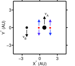
Figure 1: Example of the possible initial starting configurations. The directions of the initial velocities of the stellar components ($\nu$ Oct A and $\nu$ Oct B) are shown with black coloured arrows and appropriate labels. The proposed planet is represented by the red coloured dots in the 3 o’clock position (right) and the 9 o’clock position (left). The possible directions of the initial velocity for the planetary component are either prograde (purple) or retrograde (blue). The arrows indicate the directions in the initial configurations of the system.

The coplanar RTP indicates that the putative planet moves in the same orbital plane as the two stellar components; additionally, its mass is considered negligible. The initial orbital velocity of the planet is calculated assuming a Keplerian circular orbit about its host star; see Fig. 1 for a depiction of the initial system configuration. For simplicity we assume the $(u,w)$ components are equal to zero and the magnitude of the velocity to be in the direction of the $v$ component. The mean value of the eccentricity of the binary, $e_{b}$, is used due to accuracy of the value given. A Taylor expansion in initial orbital velocity of the binary shows that the first order correction would only change the initial orbital velocity of the respective stars by a factor of $10^{-8}$. The initial eccentricity of the planet, $e_{p}$, has been chosen to be equal to zero due to the redundancy it provides in the selection of the initial planetary position. Noting that the inclination angle of the planet, $i_{p}$, has not yet been determined, it is taken to be $90^{\circ}$ consistent with the requirement of the coplanar RTP.

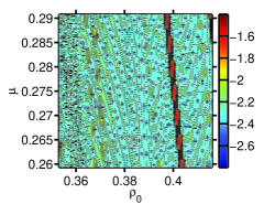
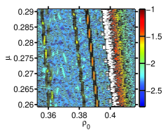
Figure 3: Same as Fig. 2, but now for retrograde planetary motion.

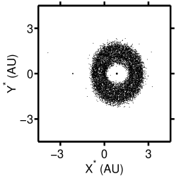
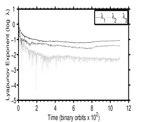
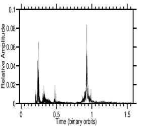
Figure 5: Case study of planetary motion with the planet placed in the 3 o’clock position and in retrograde motion. This case displays the conditions for $\mu=0.2825$ and $\rho_{0}=0.400$.

To integrate the equations of motion, a sixth order symplectic integration method is used (Yoshida, 1990). In the computation of Figs. 2 and 3 a fixed time step of $10^{-3}$ is assumed. This proved to be appropriate since the average relative error in the Jacobi constant is found to be on the order of $10^{-8}$. To increase the precision for the individual cases depicted in Figs. 5 to 9, a fixed time step of $10^{-4}$ is used, which decreased the average relative error to the order of $10^{-10}$. However, this choice entailed a considerable increase of the computation time. Therefore, the models pertaining to Fig. 2 were integrated for 10,000 binary orbits (approximately 29,000 years) and the models pertaining to Fig. 3 were integrated for 1,000 binary orbits (approximately 2,900 years), noting that this figure is considerably less than utilized in the mainframe of our study for the determination of the statistical probability of a prograde planetary configuration. Moreover, the models of Figs. 5 to 9 were integrated for 80,000 binary orbits (approximately 232,000 years).

In the treatment of this problem, four separate types of initial conditions of the system are considered. They encompass the two different starting positions of the planet with respect to the massive host star, which are: the 3 o’clock and 9 o’clock positions (see Fig. 1). With each of these starting positions, we considered the possibility of planetary motion in counter-clockwise and clockwise direction relative to the direction of motion of the secondary stellar component; the directions are referred to as prograde and retrograde, respectively. The primary masses are considered to move in ellipses about the centre of mass of the system.

2.3 Statistical Parameter Space

In the present work we will explore the role(s) of small variations in the system parameters. Notably we will investigate how the stellar mass ratio as well as the semimajor axis and inherently the eccentricity of the stellar components can change the outcome of our orbital stability simulations. Particularly when we consider the statistical probability of prograde orbits for the suggested planet. These variations are due to the observational uncertainties of the respective parameter; see Ramm et al. (2009) and Table 1 for details.

Equation (7) gives the definition of the mass ratio $\mu$ with $m_{1}=1.4\pm 0.3~{}M_{\odot}$ and $m_{2}=0.5\pm 0.1~{}M_{\odot}$. Taking $m_{1}$ and $m_{2}$ as statistically independent from one another, the bounding values for $\mu$ are $\left[0.220,0.306\right]$, i.e., $0.263\pm 0.043$. In this case, we assumed the reported uncertainty bars for the stellar masses to be $1.25~{}\sigma$, noting that through this choice $\mu$ is consistent with the mass ratio $q=0.38\pm 0.03$ derived by Ramm et al. (2009) that was used for computing $m_{2}$ based on the sum of the two masses. Formulas and methods for the propagation-of-error, which in essence employ a first-order Taylor expansion, have been given by, e.g., Meyer (1975); see also Press et al. (1986) for numerical methods if the error is calculated via a Monte-Carlo simulation.

Equation (12) gives the definition for the relative initial distance of the planet, expressed in terms of $R_{0}$ and $D$, i.e., the initial distance of the planet from its host star, the more massive of the two stars with mass $m_{1}$ and the initial distance between the two stars, respectively. This definition also allows to compute the bounding values for $\rho_{0}$. Following the assumption made by Eberle & Cuntz (2010b), the set up of the binary system will be initialized by assuming the secondary stellar component to be located in the apastron starting position, entailing that $D$ is modified as $D=a_{b}\left(1+e_{b}\right)$. Thus, the observation uncertainties of $a_{p}$, $a_{b}$, and $e_{b}$ will be utilized to compute the bounding values for $\rho_{0}$ (see Table 1). As result we obtain $\left[0.344,0.418\right]$, i.e., $0.381\pm 0.037$. These values will be considered in the subsequent set of detailed orbital stability studies by making appropriate choices for $\mu$ and $\rho_{0}$ when setting the initial conditions. The outcome of the various simulations will, in particular, allow a detailed statistical analysis of the mathematical probability for the existence of the suggested planet in a prograde orbit; see Sect. 3.3.

2.4 Stability Criteria

In our approach we employ two independent criteria. One method deals with identifying events that can cause instability, whereas the other method allows us to determine stability. First, we monitor the relative error in the Jacobi constant to detect instabilities. By monitoring this constant we can determine when the integrator loses its accuracy or fails completely. It has been shown that this method is particularly sensitive to close approach events of the planet with any of the stellar components. However, it has previously been shown by Eberle, Cuntz & Musielak (2008) and Eberle & Cuntz (2010a) that these close approach events are preceded by an encounter with the so-called “zero velocity contour” (ZVC) for the coplanar circular RTP.

Generalizing this criteria to the elliptic RTP, an analogous “zero velocity function” (ZVF) can be found that is, however, dependent on the initial distance between the stellar components (Szebehely, 1967). The ZVF can also be described by a pulsating ZVC; see Szenkovits & Makó (2008) for updated results. Note that the ZVC will be largest when the binary components are at apastron and smallest when they are at periastron. Noting that we choose the stars to be at the apastron starting position, the largest ZVC is inherently defined as well. When the planetary body encounters the ZVC, the orbital velocity decreases dramatically, which reduces the $\dot{u}$ and $\dot{v}$-related forces. As a result, the planetary body follows a trajectory that results in a close approach. This behaviour provides an indication that the system will eventually become unstable, resulting in an ejection of the planetary body from the system (most likely outcome) or its collision with one of the stellar components (less likely outcome).

The second criterion utilizes the method of Lyapunov exponents (Lyapunov, 1907), which is commonly used in nonlinear dynamics for determining the onset of chaos in different dynamical systems (e.g., Hilborn, 1994; Musielak & Musielak, 2009). A numerical algorithm that is typically adopted for calculating the spectrum of Lyapunov exponents was originally developed by Wolf et al. (1985). In this approach, a set of tangent vectors $\textbf{x}_{i}$ and their derivatives $\dot{\textbf{x}}_{i}$ with $i=1,\ldots,6$ are introduced and initialized. In our approach, we choose all tangent vectors to be unit vectors for simplicity, and use a standard integrator akin to the Runge-Kutta schemes for computing changes in the tangent vectors within each timestep. After the tangent vectors become oriented along the flow, it is necessary to perform a Gram-Schmidt Renormalization (GSR) to orthogonalize the tangent space. In this specific procedure, we calculate a new orthonormal set of tangent vectors here denoted by primes ($\prime$), and obtain

$$\textbf{x}_{1}^{{}^{\prime}} = {\textbf{x}_{1}\over\left\|\textbf{x}_{1}\right\|}$$ (13)

$$\textbf{x}_{2}^{{}^{\prime}} = {\textbf{x}_{2}-\left\langle\textbf{x}_{2},\>\textbf{x}_{1}^{{}^{\prime}}\right\rangle\textbf{x}_{1}^{{}^{\prime}}\over\left\|\textbf{x}_{2}-\left\langle\textbf{x}_{2},\>\textbf{x}_{1}^{{}^{\prime}}\right\rangle\textbf{x}_{1}^{{}^{\prime}}\right\|}$$ (14)

$$\vdots$$

$$\textbf{x}_{6}^{{}^{\prime}} = {\textbf{x}_{6}-\left\langle\textbf{x}_{6},\>\textbf{x}_{5}^{{}^{\prime}}\right\rangle\textbf{x}_{5}^{{}^{\prime}}-\ldots-\left\langle\textbf{x}_{6},\>\textbf{x}_{1}^{{}^{\prime}}\right\rangle\textbf{x}_{1}^{{}^{\prime}}\over\left\|\textbf{x}_{6}-\left\langle\textbf{x}_{6},\>\textbf{x}_{5}^{{}^{\prime}}\right\rangle\textbf{x}_{5}^{{}^{\prime}}-\ldots-\left\langle\textbf{x}_{6},\>\textbf{x}_{1}^{{}^{\prime}}\right\rangle\textbf{x}_{1}^{{}^{\prime}}\right\|}$$ (15)

With this new set of tangent vectors, the spectrum of Lyapunov exponents is computed by using

$$\lambda_{i}\ =\ {1\over\tau}\left[\lambda_{i-1}+\log\left\|\textbf{x}_{i}-\sum_{j=1}^{i}{\left\langle\textbf{x}_{i},\>\textbf{x}_{j-1}^{{}^{\prime}}\right\rangle\textbf{x}_{j-1}^{{}^{\prime}}}\right\|\right]$$ (16)

where $\lambda_{o}=\textbf{x}_{o}^{{}^{\prime}}=0$.

The Lyapunov exponents have extensively been used in studies of orbital stability in different settings pertaining to the Solar System (e.g., Lecar, Franklin & Murison, 1992; Milani & Nobili, 1992; Lissauer, 1999; Murray & Holman, 2001). Typically, the maximum Lyapunov exponent (MLE) is adopted as a measure of the rate with which nearby trajectories diverge. The reason is that the MLE offers the unique measure of the largest divergence. We previously used the MLE criterion to provide a cutoff for which stability can be assured given the behaviour of the MLE in time. This cutoff value has previously been determined by Quarles et al. (2011); it is given as log $\lambda_{\rm max}=-0.82$ on a logarithmic scale of base 10.

Recalling that the cutoff in MLE is inversely related to the Lyapunov time $t_{\rm L}$, the latter provides an estimate of the predictive period for which stability is guaranteed. The lower (i.e., more negative) the logarithmic value of the MLE, the longer the time for which orbital stability will be ensured. Due to the finite time of integration, this estimate is only valid for the integration timescale considered. But the nature of how the MLE changes in time will provide the evidence to whether the MLE is asymptotically decreasing and thereby allowing to identify orbital stability. Hence this cutoff will be used for establishing orbital stability of the suggested planet in the $\nu$ Octantis system.

Table 2: Survival Counts of the Suggested Planet in $\nu$ Octantis for 1,000 binary orbits.

Configuration		Unstable Count	Stable Count	Stable Percentage
Prograde	3 o’clock	17544	1776	9.2 %
Prograde	9 o’clock	19200	120	0.6 %
Retrograde	3 o’clock	1040	19184	94.9 %
Retrograde	9 o’clock	0	20224	100 %

3 Results and Discussion

3.1 Model Simulations

In the following we report the general behaviour of stability for the set of orbital stability simulations pursued in our study. Our initial focus is on the MLE. In Figs. 2 and 3, the various values of the MLE as a function of $\mu$ and $\rho_{0}$ are denoted using a colour code. The range of colours shows that dark red represents a relatively high (less negative) logarithmic MLE value, whereas dark blue represents a relatively low (more negative) logarithmic MLE value. The white background represents conditions, which failed to complete the respective allotted run time; see Sect. 2.4 for a discussion of possible conditions for terminating a simulation.

Figure 2 shows the result of our simulations for 10,000 binary orbits, i.e., about 29,000 years, in the prograde configuration for starting conditions given by the 3 o’clock or 9 o’clock planetary position. The results were obtained using values of $\mu$ between 0.220 and 0.306 in increments of 0.001. Concerning the initial conditions in $\rho_{0}$, denoting the relative starting position of the planet, we use values between 0.272 and 0.502 in increments of 0.001. We show the $1\sigma$ region in $\rho_{0}$ between 0.344 and 0.418 where $\nu$ Oct is proposed to exist by a grey shaded region; see Sect. 2.3. Between the two bounding values regarding $\rho_{0}$, there exists a region of stability as well as a marginal stability limit. The limit of marginal stability is consistent with previous findings by Holman & Wiegert (1999) for the case with the planetary eccentricity taken into account. This region of marginal stability is more pronounced in the 3 o’clock starting configuration; it begins at $\rho_{0}\approx 0.315$. The marginal stability region decreases as $\mu$ increases, which is expected because the perturbing mass is becoming more significant as the mass ratio $\mu$ increases. There is a noticeable favoritism towards the 3 o’clock starting position as indicated by the survival counts given in Table 2. This outcome is expected as the perturbing mass exerts a lesser force on the planet if initially placed at the 3 o’clock position.

Figure 3 shows the result for the retrograde configuration for 1,000 binary orbits considering both the 3 o’clock and 9 o’clock planetary starting positions. Due to the larger number of conditions that survived during this time interval we have reduced the bounds of initial conditions following the bounding values of Eberle & Cuntz (2010b). Here the bounding values for $\mu$ are given as 0.2593 and 0.2908 with increments of 0.0001. The increment in $\mu$ was reduced to allow better insight into the role of chaos in this type of configuration. The initial conditions of $\rho_{0}$ begin with 0.353 and end with 0.416 in increments of 0.001, which allows to cover the most pronounced features of the retrograde configuration.

Figure 3 demonstrates a broad region of stability within the selected parameter space. The 9 o’clock starting position has many regions of bounded chaos. These regions of bounded chaos exhibit locally less negative values for MLE, which however do not exceed the previously determined cutoff value of log $\lambda_{\rm max}=-0.82$; see Sect. 2.4. The nature of these orbits and the connection to the MLE will be discussed in Sect. 3.2. The greatest region of bounded chaos is obtained for $\rho_{0}\approx 0.41$. This region decreases in $\rho_{0}$ as $\mu$ increases for the same reason as the change in the marginal stability limit in Fig. 2. The 3 o’clock starting position shows similar features but there exists a region of instability with this starting position at $\rho_{0}\approx 0.41$. This region coincides with the extended region of bounded chaos in the 9 o’clock starting position. The nature of this region can be deduced from the parameters given by Ramm et al. (2009); see Table 1. There exists a 5:2 resonance of the planet with the binary that places the suggested planet moving towards the barycentre at the periastron point of the binary inducing an instability. For the 9 o’clock position the suggested planet would be moving away which would provide a large perturbation but insufficient for producing an instability.

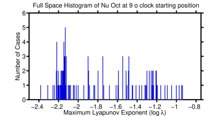
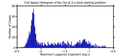
Figure 4: Histograms of configurations that survived 1000 binary orbits in prograde motion. Note the significant difference in scale regarding both the $x$ and $y$-axis.

Figure 4 provides the histograms of simulations pertaining to both starting positions for the prograde configuration. These histograms indicate the number of surviving cases related to the array of initial conditions for the parameter space detailed in Fig. 2. The bin width is 0.01 in the logarithmic MLE scale, corresponding to $1.47\times 10^{-4}$ in the linear MLE scale. Although there is not a case that survives 10,000 binary orbits in the 1 $\sigma$ region, we provide these histograms to demonstrate what different initial conditions entail near the lower and upper uncertainty limits. Figure 2 shows that all the surviving cases cluster towards the lower bound in $\rho_{0}$. Furthermore, it is obtained that the 9 o’clock starting position has far fewer surviving initial conditions than the 3 o’clock starting position. This is also reflected in the histograms. The histogram of the 9 o’clock position is sparse; without the aid of the 3 o’clock histogram there would be too few counts to provide substantial information. But inspecting the 3 o’clock histogram reveals that there is a Gaussian-type distribution about the logarithmic MLE value of $-2.2$. This indicates that for the limited simulation time adopted for this part of our study, there is a very small number of cases indicating stability for the prograde configuration. However, these cases are near the $2\sigma$ or $3\sigma$ limit concerning the permitted values of the planetary position $\rho_{0}$ as discussed in Sect. 3.3.

3.2 Case Studies

In the following we probe some orbits of retrograde configurations in more detail; see Figs. 5 to 9 for information. These figures show from left to right the respective orbital diagram in a rotating reference frame, the associated Lyapunov spectrum, and the Fourier periodogram. Through these diagrams we can assess the nature of these orbits to determine stability and measure the chaos within the system.

Figure 5 with $(\mu,\rho_{0})=(0.2825,0.400)$ is provided to show a case of instability. In this case we find that the orbit presents itself as a wide annulus and already at first glance appears chaotic. The Lyapunov spectrum reveals that the MLE levels off at log $\lambda=-1$ fairly quickly, which is near the proposed cutoff value for unstable chaotic behaviour. For the timespan between 300 and 800 binary orbits, the MLE fluctuates until it finally pushes upward to $\lambda_{\rm max}$. The Fourier periodogram shows that this case is truly chaotic due to the amount of noise presented by the periodogram. There are many periods which may promote the outcome of instability via resonance overlap (e.g., Mudryk & Wu, 2006; Mardling, 2007). The proposed planet is approaching the barycentre when the binary is at its periastron position, which should be considered the main cause of this instability.

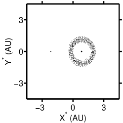
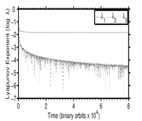
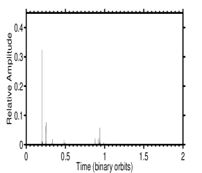
Figure 6: Case study of planetary motion with the planet placed in the 3 o’clock position and in retrograde motion. This case displays the conditions for $\mu=0.2805$ and $\rho_{0}=0.358$.

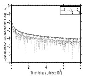
Figure 7: Case study of planetary motion with the planet placed in the 3 o’clock position and in retrograde motion. This case displays the conditions for $\mu=0.2630$ and $\rho_{0}=0.374$.

Figures 6 and 7 with $(\mu,\rho_{0})=(0.2805,0.358)$ and $(0.2630,0.374)$, respectively, exhibit similar features between each other in the orbit diagram and periodogram. However, there is a difference in the respective Lyapunov spectra. Both cases show trends of stability, although Fig. 6 demonstrates bounded chaos. It presents a different nature than the previous case of instability (see Fig. 5) as the MLE settles near log $\lambda=-1.8$ and does not fluctuate enough to reach $\lambda_{\rm max}$. Both cases given as Figs. 6 and 7 represent orbits that form annuli; however, the annulus widths are less than that of the unstable case depicted in Fig. 5. They are thus classified as stable with Fig. 6 being chaotic and Fig. 7 being non-chaotic.

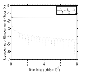
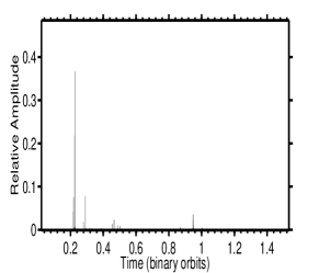
Figure 8: Case study of planetary motion with the planet placed in the 9 o’clock position and in retrograde motion. This case displays the conditions for $\mu=0.2696$ and $\rho_{0}=0.401$.

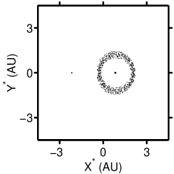
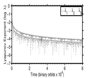
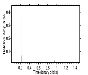
Figure 9: Case study of planetary motion with the planet placed in the 9 o’clock position and in retrograde motion. This case displays the conditions for $\mu=0.2780$ and $\rho_{0}=0.388$.

Figures 8 and 9 with $(\mu,\rho_{0})=(0.2696,0.401)$ and $(0.2780,0.388)$, respectively, reveal similar features compared to the previous set of figures regarding all three diagrams. These cases are provided to demonstrate the similarities between the 3 o’clock starting positions depicted in Figs. 6 and 7 and the 9 o’clock starting positions depicted in Figs. 8 and 9. The comparison between Figs. 6 and 8 indicates a similar orbit diagram and periodogram, but the limiting values of the MLE settle at a slightly more negative value in Fig. 6. Figures 7 and 9 supply similar orbital diagrams but there are minor differences in the periodograms and Lypaunov spectra. These figures display the same behaviour in MLE but there is a difference in the periodic nature of the decrease in MLE, which is also revealed by the difference in the number of peaks in the corresponding periodograms.

Table 3: Statistical Probability of Prograde Planetary Orbits^a.

Mass Ratio	9 o’clock Position		3 o’clock Position
$\mu$	$\sigma$	Probability (%)	$\sigma$	Probability (%)
0.306	$\ldots$	$\ldots$	2.30	1.1
0.263	$\ldots$	$\ldots$	2.11	1.7
0.220	2.95	0.16	1.89	2.9

1. Based on 10,000 binary orbits; see Fig. 2

3.3 Statistical Analysis of Orbital Stability

A significant component of the present study is to provide a statistical analysis regarding whether or not the suggested planet in the $\nu$ Octantis system is able to exist in a prograde or retrograde orbit. Previously, we reported on the general behaviour of orbital stability for the set of simulations with focus on the MLE (see Sect. 2.4). In Figs. 2 and 3, the various values of the MLE were given as function of the mass ratio $\mu$ and the initial planetary distance parameter $\rho_{0}$. The bounding values for $\mu$ were given as $\left[0.220,0.306\right]$, i.e., $0.263\pm 0.043$, and for $\rho_{0}$ as $\left[0.344,0.418\right]$, i.e., $0.381\pm 0.037$. We found that based on the MLE as well as a number count of surviving cases (see Sect. 3.1) that the existence of the suggested planet in a retrograde orbit is almost certainly possible, whereas in a prograde orbit it is virtually impossible.

For prograde orbits based on the “landscape of survival” (see Fig. 2), another type of analysis can be given, see Table 3. We conclude that for the 9 o’clock planetary starting position and for a relatively high stellar mass ratios, i.e., $\mu\mathrel{\hbox to0.0pt{\lower 3.0pt\hbox{$\mathchar 536\relax$}\hss}\raise 2.0pt\hbox{$\mathchar 318\relax$}}0.25$, the planet must start very close to the star, i.e., that the associated probability for $\rho_{0}$ is way outside the statistical $3\sigma$ limit. Only for relatively small stellar mass ratios, i.e., $\mu\simeq 0.22$, the planetary starting distance $\rho_{0}$ would be barely consistent with the $3\sigma$ limit, amounting to a statistical probability of 0.16%. For a 3 o’clock planetary starting position, these probabilities pertaining to the permitted values of $\rho_{0}$ are moderately increased. It is found that the associated probabilities for $\mu$ given as 0.306, 0.263, and 0.220 are 1.1%, 1.7%, and 2.9%, respectively.

Moreover, it should be noted that this statistical analysis refers to a “landscape of survival” that has been obtained for a timespan of 10,000 binary orbits, corresponding to 29,000 years. An analysis of the evolution of that landscape shows that it tends to dissipate if larger timespans are adopted. Even for timespans of 10,000 binary orbits, there are many parameter combinations $(\mu,\rho_{0})$ where, concerning prograde orbits, no orbital stability is found even if $\rho$ values are chosen at or beyond the statistical $3\sigma$ level.

Another perspective is offered through Fig. 10, which provides additional insight into the statistical nature of our simulations. It addresses the view of long term stability. Figure 10 depicts two curves representing the number of surviving configurations as a function of time for each starting position in the prograde configuration. The features of this logarithmic plot show us that for the first 10 binary orbits there is not a preference towards stability of either starting position. After 10 binary orbits the 9 o’clock position shows a significantly steeper trend of instability as indicated by the slope of the respective curve. The 3 o’clock position also shows a trend toward instability but it is asymptotically approaching a limit of 10³ much more smoothly. With these limits, we can estimate the likelihood for a prograde planetary configuration to be extremely small in the framework of long-term simulations. However, for a very large range of $(\mu,\rho_{0})$ combinations, the stability of retrograde planetary configuration appears almost certainly guaranteed, even for timescales beyond $10^{5}$ binary orbits.

4 Conclusions

This study offers detailed insights into the principal possibility of prograde and retrograde orbits for the suggested planet in the $\nu$ Octantis system, if confirmed through future observations. A previous study by Eberle & Cuntz (2010b) concluded that the planet is most likely stable if assumed to be in a retrograde orbit with respect to the secondary system component. In the present work, we were able to confirm this theoretical finding, while taking into account the observationally deduced uncertainty ranges of the orbital parameters for the stellar components and the suggested planet as well as different mass ratios of the stellar components.

In addition, we also employed additional mathematical methods, particularly the behaviour of the maximum Lyapunov exponent (MLE). We found that virtually all cases of prograde orbit became unstable over a short amount of time; the best cases for survival (although barely significant in a statistical framework) were found if a relatively small mass ratio for the two stellar components was assumed and if the initial configuration was set for the planet to start at the 3 o’clock position. This later preference is also consistent with previous general results by Holman & Wiegert (1999) and others.

Thus, our results of the retrograde simulations indicate a high probability for stability within this type of configuration. Moreover, this configuration displays regions in the system where bounded chaos can exist due to the resonances present. Concerning retrograde orbits, there is little preference for the planetary starting position. In summary, we conclude that the $\nu$ Octantis star–planet system is an interesting case for future observational and theoretical studies, including additional long-term orbital stability analyses if the suggested planet is confirmed by follow-up observations.

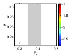
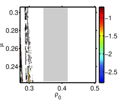
Figure 2: Detailed results of simulations for the parameter space for the case of prograde planetary motion. The left and right panel represent the simulations with the planet initially placed at the 9 o’clock and 3 o’clock position, respectively. The grey area represents the statistical $1\sigma$ range in $\rho_{0}$, which is $0.381\pm 0.037$.

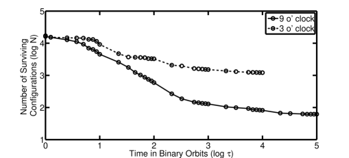
Figure 10: Logarithmic representation of the surviving number of configurations (prograde orbits) as function of time given in units of completed binary orbits.

References

- Anderson et al. (2010) Anderson D. R., et al., 2010, ApJ, 709, 159
- Allende Prieto & Lambert (1999) Allende Prieto C., Lambert D. L., 1999, A&A, 352, 555
- Baker & Gollub (1990) Baker G. L., Gollub J. P., 1990, Chaotic Dynamics: An Introduction. Cambridge Univ. Press, Cambridge
- Benettin et al. (1980) Benettin G., Galgani L., Giorgilli A., Strelcyn J.-M., 1980, Meccanica, 15, 9
- Cuntz, Eberle & Musielak (2007) Cuntz M., Eberle J., Musielak, Z. E., 2007, ApJ, 669, L105
- Drilling & Landolt (2000) Drilling J. S., Landolt A. U., 2000, in A. N. Cox, ed., Allen’s Astrophysical Quantities, 4th edn. Springer-Verlag, New York, p. 381
- Eberle & Cuntz (2010a) Eberle J., Cuntz M., 2010a, A&A, 514, A19
- Eberle & Cuntz (2010b) Eberle J., Cuntz M., 2010b, ApJ, 721, L168
- Eberle, Cuntz & Musielak (2008) Eberle J., Cuntz M., Musielak Z. E., 2008, A&A, 489, 1329
- Eggenberger, Udry & Mayor (2004) Eggenberger A., Udry S., Mayor M., 2004, A&A, 417, 353
- ESA (1997) European Space Agency, 1997, SP-1200, The Hipparcos and Tycho Catalogues. ESA, Noordwijk
- Fatuzzo et al. (2006) Fatuzzo M., Adams F. C., Gauvin R., Proszkow E. M., 2006, Publ. Astron. Soc. Pac., 118, 1510
- Gonczi & Froeschlé (1981) Gonczi R., Froeschlé C., 1981, Cel. Mech. Dyn. Astron., 25, 271
- Hilborn (1994) Hilborn R. C., 1994, Chaos and Nonlinear Dynamics, Oxford Univ. Press, Oxford
- Holman & Wiegert (1999) Holman M. J., Wiegert P. A., 1999, AJ, 117, 621
- Houk & Cowley (1975) Houk N., Cowley A. P., 1975, University of Michigan Catalogue of Two-Dimensional Spectral Types for the HD Stars, Vol. 1. Univ. of Michigan, Ann Arbor
- Jefferys (1974) Jefferys W. H., 1974, AJ, 79, 710
- Lecar, Franklin & Murison (1992) Lecar M., Franklin F., Murison M., 1992, AJ, 104, 1230
- Lin, Bodenheimer & Richardson (1996) Lin D. N. C., Bodenheimer P., Richardson D. C., 1996, Nature, 380, 606
- Lissauer (1993) Lissauer J. J., 1993, Ann. Rev. Astron. Astrophys., 31, 129
- Lissauer (1999) Lissauer J. J., 1999, Rev. Mod. Phys., 71, 835
- Lyapunov (1907) Lyapunov M. A., 1907, Ann. Fac. Sci., University Toulouse, 9, 203
- Meyer (1975) Meyer S. L., 1975, Data Analysis for Scientists and Engineers, Wiley, Hoboken, NJ
- Mardling (2007) Mardling R. A., 2007, in Vesperini E., Giersz M., Sills A., eds, Dynamical Evolution of Dense Stellar Systems, Proc. IAU Symp. 246, p. 199
- Milani & Nobili (1992) Milani A., Nobili A. M., 1992, Nature, 357, 569
- Morais & Correia (2012) Morais M. H. M., Correia A. C. M., 2012, MNRAS, in press (arXiv:1110.3176)
- Mudryk & Wu (2006) Mudryk L. R., Wu Y., 2006, ApJ, 639, 423
- Murray & Holman (2001) Murray N., Holman M., 2001, Nature, 410, 773
- Musielak & Musielak (2009) Musielak Z. E., Musielak D. E., 2009, Int. J. Bifurcation and Chaos, 19, 2823
- Press et al. (1986) Press W. H., Flannery B. P., Teukolsky S. A., Vetterling W. T., 1986, Numerical Recipes, Cambridge University Press, Cambridge, UK
- Quarles et al. (2011) Quarles B., Eberle J., Musielak Z. E., Cuntz M., 2011, A&A, 533, A2
- Queloz et al. (2010) Queloz D., et al., 2010, A&A, 517, L1
- Raghavan et al. (2006) Raghavan D., et al., 2006, ApJ, 646, 523
- Ramm et al. (2009) Ramm D. J., Pourbaix D., Hearnshaw J. B., Komonjinda S., 2009, MNRAS, 394, 1695
- Sato et al. (2003) Sato B., et al., 2003, ApJ, 597, L157
- Smith & Szebehely (1993) Smith R. H., Szebehely V., 1993, Cel. Mech. Dyn. Astron., 56, 409
- Szebehely (1967) Szebehely V., 1967, Theory of Orbits. Academic Press, New York and London
- Szenkovits & Makó (2008) Szenkovits F., Makó Z., 2008, Cel. Mech. Dyn. Astron., 101, 273
- van Leeuwen (2007) van Leeuwen F., 2007, A&A, 474, 653
- Winn et al. (2009) Winn J. A., et al., 2009, ApJ, 703, L99
- Wolf et al. (1985) Wolf A., Swift J. B., Swinney H. L., Vastano J. A., 1985, Physica D, 16, 285
- Yeager, Eberle & Cuntz (2011) Yeager K. E., Eberle J., Cuntz M., 2011, Int. J. Astrobiol., 10, 1
- Yoshida (1990) Yoshida H., 1990 Phys. Lett. A, 150, 262