Beresinskii-Kosterlitz-Thouless transition within the sine-Gordon approach: the role of the vortex-core energy

Abstract

One of the most relevant manifestations of the Beresinskii-Kosterlitz-Thouless transition occurs in quasi-two-dimensional superconducting systems. The experimental advances made in the last decade in the investigation of superconducting phenomena in low-dimensional correlated electronic systems raised new questions on the nature of the BKT transitions in real materials. A general issue concerns the possible limitations of theoretical predictions based on the $XY$ model, that was studied as a paradigmatic example in the original formulation. Here we review the work we have done in revisiting the nature of the BKT transition within the general framework provided by the mapping into the sine-Gordon model. While this mapping was already known since long, we recently emphasized the advantages on such an approach to account for new variables in the BKT physics. One such variable is the energy needed to create the core of the vortex, that is fixed within the $XY$ model, while it attains substantially different values in real materials. This has interesting observable consequences, especially in the case when additional relevant perturbations are present, as a coupling between stacked two-dimensional superconducting layers or a finite magnetic field.

I Introduction

Almost 40 years after the pioneering work by Beresinskii berezinsky and Kosterlitz and Thouless kosterlitz_thouless ; kosterlitz_renormalization_xy the Beresinskii-Kosterlitz-Thouless (BKT) transition is still the subject of an intense experimental and theoretical research. On very general grounds, what makes it so fascinating is the possibility of a phase transition that is not driven by the explicit breaking of a given symmetry, but is based on the emergence of a finite (and measurable) rigidity of the system. The BKT transition was originally formulated within the context of the two-dimensional (2D) $XY$-model, which describes the exchange interaction between classical two-component spins with fixed length $S=1$:

$$H_{XY}=-J\sum_{\langle ij\rangle}\cos(\theta_{i}-\theta_{j}),$$ (1)

where $J$ is the spin-spin coupling constant and $\theta_{i}$ is the angle that the $i$-th spin form with a given direction, and $i$ are the sites of a square lattice. This model admits a continuous $U(1)$ symmetry (encoded in the transformation $\theta_{i}\rightarrow\theta_{i}+\chi$), that cannot be broken at finite temperature by an average magnetization $\langle{\bf S}\rangle=\langle e^{i\theta}\rangle$ different from zero because of the Mermin-Wagner theorem. Nonetheless, the system can become “stiff” at low temperature with respect to fluctuations of the $\theta$ variable, leading to a power-law decay of the spin correlation functions, i.e. $\langle e^{i(\theta(i)-\theta(0))}\rangle\simeq r^{-T/2\pi J}$, in contrast to the exponential one expected in the truly disordered state. Such a change of behavior cannot be “smooth”, i.e. a phase transition occurs in between, which appears to be controlled by the emergence of vortex-like excitations. The original argument used if Ref. kosterlitz_thouless, to capture the temperature scale of such a transition is rather intuitive: in two dimensions both the energy $E$ and the entropy $S$ of a single vortex excitation depend logarithmically on the size $L$ of the system, so that the free energy reads:

$$F=E-TS=(\pi J-2T)\ln\frac{L}{a}.$$ (2)

As a consequence, at temperatures larger than

$$T_{BKT}\simeq\frac{\pi J}{2},$$ (3)

free vortices start to proliferate and destroy the quasi-long-ranged order of the correlation functions.

As it was observed already in the original paperskosterlitz_thouless ; kosterlitz_renormalization_xy , several physical phenomena are expected to belong to the same universality class than the $XY$ model (1), as for example the superfluid transition in two dimensions. Later on it was realized that the same idea can be applied also to superconducting (SC) thin filmsdoniach_films ; halperin_ktfilms , even though in the charged superluid the logarithmic interaction between vortices is screened by the supercurrents at a finite distance $\Lambda=\lambda^{2}/d$, where $\lambda$ is the penetration depth of the magnetic field and $d$ is the film thickness.pearl In practice, for sufficiently thin films with large disorder (so that $\lambda$ is also large) the electromagnetic screening effects are weak enough to expect the occurrence of the BKT transition.

As a matter of fact, the case of SC thin films represented one of the most studied applications of the BKT physics. In principle, in this case one has also several possibilities to access experimentally the specific signatures of the BKT physics. For example, by approaching the transition from below, the superfluid density $n_{s}$ is expected to go to zero discontinuously at the BKT temperature $T_{BKT}$, with an “universal” relation between $n_{s}(T_{BKT})$ and $T_{BKT}$ itselfnelson_univ_jump_prl77 ; review_minnaghen ; giamarchi_book_1d , that is the equivalent of the relation (3), since $J\propto n_{s}$ (see Eq. (5) below). Approaching instead the transition from above one has in principle the possibility to identify the BKT transition from the temperature dependence of the SC fluctuations. Indeed, in 2D the temperature dependence of both the paraconductivity $\Delta\sigma\equiv\sigma-\sigma_{n}$ and the diamagnetism $\chi_{d}$ is encoded in the SC correlation length $\xi(T)$,halperin_ktfilms which increases approaching the transitions due to the increase of SC fluctuations:

$$\Delta\sigma\propto\xi^{2}(T),\quad\chi_{d}\propto-\xi^{2}(T).$$ (4)

Within BKT theory $\xi(T)$ diverges exponentially at $T_{BKT}$ as $\xi_{BKT}(T)\simeq ae^{b/\sqrt{t}}$,kosterlitz_renormalization_xy ; review_minnaghen where $t=T/T_{BKT}-1$, in contrast to the power-law $\xi_{GL}(T)\simeq 1/(T-T_{c})$ expected within Ginzburg-Landau (GL) theoryvarlamov_book . As a consequence, by direct inspection of the paraconductivity or diamagnetism near the transition one could identify the occurrence of vortex fluctuations, which lead to an exponential temperature dependence of the SC correlation length.

Quite interestingly, very direct measurements of the BKT universal jump in the superfluid density of SC films became available only recently,lemberger_InO ; martinoli_films ; lemberger_bilayer ; pratap_apl10 ; pratap_bkt_prl11 ; lemberger_Bifilms_cm11 due to the improvement of the experimental techniques, triggered mostly by the investigation of high-temperature superconductors in the late nineties. In particular, the use of the two-coil mutual inductance techniquelemberger_twocoils turned out to be crucial to obtain the absolute value of the superfluid density at zero temperature, which is needed to compare the experimental data with the BKT predictions. Recently a great deal of information has come also from Tera-hertz spectroscopyarmitage_films_prb07 ; armitage_InO_prb11 ; armitage_natphys11 , which probes the finite-frequency analogous of the superfluid-density jump. At the same time, in the last decade new 2D or quasi-2D SC systems emerged where the BKT transition is expected to occur. To this category belong for example the nanometer-thick layers of SC electron systems formed at the interface between artificial heterostructures made of insulating oxides as LaAlO₃/SrTiO₃triscone_science07 ; triscone_nature08 or LaTiO₃/SrTiO₃biscaras_natcomm10 , or at the liquid/solid interface of field-effect transistors made with organic electrolytesiwasa_natmat10 . A second remarkable example is provided by layered 3D systems as cuprate high-temperature superconductors, where the weak interlayer coupling makes it plausible that at least in same regions of the phase diagram a BKT transition could be at playemery ; review_lee . Even though the existence of a BKT transition in bulk (3D) samples is still controversial, as we shall discuss below, nonetheless in cuprates the proximity of the SC phase to the Mott insulator leads to a large penetration depth without need of introducing strong disorder, making in principle thin-films of cuprate superconductors the best candidate to study BKT physicscorson_nature99 ; martinoli_films ; triscone_fieldeffect ; lemberger_bilayer ; lemberger_Bifilms_cm11 ; armitage_natphys11 . Recently, much attention has been devoted also to artificial heterostructures made of cuprates at different doping levelyuli_prl08 ; bozovic_science09 , where the observation of BKT physics in the SC films is complicated even more by the proximity to the non-SC correlated insulator.

A common characteristic of the cases mentioned above is that the BKT transition is expected to occur in systems where electronic correlations are not necessarily in the weak-coupling limit. This can be due to the presence of strong disorder, as it is the case for thin disordered films of conventional superconductors, to the artificial spatial confinement, as in the SC interfaces, or to the intrinsic nature of the system, as it occurs in cuprate superconductors. As a consequence, several experimental results seem to point towards a kind of “unconventional” BKT physics, which needs to be addressed using a wider perspective than the one proposed in the original formulation. A paradigmatic example of an apparent failure of the standard BKT approach is posed by recent measurements of the universal superfluid-density jump in InOarmitage_films_prb07 ; armitage_InO_prb11 and NbNpratap_apl10 ; pratap_bkt_prl11 films. In a quasi-2D superconductor of thickness $d$ the energy scale corresponding to the coupling $J$ of the $XY$ model (1) is the so-called superfluid stiffness, which is connected to the (areal) density of superfluid electrons $\rho_{s}^{2d}\equiv n_{s}d$, which in turn is measured via the inverse penetration depth $\lambda$ of the magnetic field:

$$J=\frac{\hbar^{2}\rho_{s}^{2d}}{4m}=\frac{\hbar^{2}c^{2}d}{16\pi e^{2}\lambda^{2}}.$$ (5)

This coupling has itself a bare temperature dependence $J(T)$ due to the presence of quasiparticle excitations: however, one would expect that at a temperature scale corresponding to the relation (3) free vortices start to proliferate, so that $n_{s}(T)$ jumps discontinuously to zero. In the experiments of Ref. pratap_apl10, ; pratap_bkt_prl11, one can clearly see that as the film thickness decreases $n_{s}(T)$ starts to deviate abruptly from its BCS temperature dependence. However, such a deviation seems to occur at a temperature lower than the one predicted by Eq. (3). The same observation holds for finite-frequency measurements of $n_{s}(T)$ in InO filmsarmitage_films_prb07 ; armitage_InO_prb11 , casting some doubt on that “universal” relation between the superfluid density and the critical temperature that is one of the hallmarks of the BKT transition.

It is worth noting that while the measurement of the superfluid-density behavior gives access to the most straightforward manifestation of BKT physics, its identification via SC fluctuations is much more subtle. Indeed, according to the general result (4), one needs in this case a controlled procedure to first extract the SC fluctuations contribution, and then to fit it with the BKT expression for the correlation length. Such a procedure is in general applied to the paraconductivity, even though much care should be used to disentangle GL from BKT fluctuations, as it has been discussed in a seminal paper long ago by Halperin and Nelsonhalperin_ktfilms (HN). Indeed, the BKT fit should be applied only in the region between the BCS mean-field temperature $T_{c}$ and the true $T_{BKT}$, that do not differ considerably in thin films of conventional superconductors. In contrast, recent applications to paraconductivity measurements in thin films of cuprate superconductorstriscone_fieldeffect or in SC interfacestriscone_science07 ; schneider_finitesize09 seem to suggest that in these systems the whole fluctuation regime above $T_{BKT}$ is dominated by BKT vortex fluctuations, and deviations only occur near the transition because of finite-size effect. Also in this case, one would like to distinguish unconventional effects due possibly to the nature of the underlying system, from spurious results due to an incorrect application of BKT theory. As we discussed recently in Ref. [benfatto_kt_interfaces, ] a BKT fit of the paraconductivity must be done taking into account from one side the existence of unavoidable constraints on the values of the fitting parameters, and from the other side the existence of inhomogeneity on mesoscopic scales, that can partly mask the occurrence of a sharp BKT transition. A very interesting example of application of such a procedure has been recently provided by NbN thin filmspratap_bkt_prl11 , where the direct comparison between superfluid-density data below $T_{BKT}$ and resistivity data above $T_{BKT}$ provided a paradigmatic example of BKT transition in a real system.

The issue of the inhomogeneity emerges also within the context of high-temperature cuprate superconductors. It is worth noting that in the literature the discussion concerning the occurrence of BKT physics in these layered anisotropic superconductors has been often associated to a somehow related issue, i.e. the nature of the pseudogap state above $T_{c}$. Indeed, despite the intense experimental and theoretical research devoted to it, no consensus has been reached yet concerning its origin, with two main lines of interpretation based either on a preformed-pair scenario, or on the existence of a competing order, associated to fluctuations in the particle-hole channelreview_lee . The preformed-pair scenario has in turn triggered the attention on the role of SC phase fluctuations, which are expected to be very soft in these materials having a small superfluid density. Finally, the experimental observation of a large Nerst effectong_nerst_prb06 ; ong_natphys07 ; li_nerst_prb10 and diamagnetismli_magn_epl05 ; li_nerst_prb10 ; rigamonti_prb10 well above $T_{c}$ has been used to support the notion that phase fluctuations have a vortex-like character, as it is indeed the case within the BKT picture. However, the overall interpretation of the experimental data in terms of BKT physics is not so straightforward, despite several theoretical attempts based both on the mapping into the Coulomb-gas problemsondhi_kt ; huse_prb08 or on numerical simulations for the $XY$ model.podolsky_prl07 On the other hand, a large Nerst effect arises also from the Fermi-surface reconstruction associated to stripe order taillefer_nerst09 , or from ordinary GL fluctuations,varlamov_prb11 as observed for example in thin films of conventional superconductorslesueur_nerst . Moreover, while the SC fluctuations contribution to the diamagnetism seems to fit the BKT behavior of the SC correlation lengthli_magn_epl05 , the paraconductivity shows usually more direct evidence of GL fluctuationsleridon_prb07 ; rullier-albenque_prb11 . Also the issue of the superfluid-density jump is controversial: while it has been clearly identified in very thin filmslemberger_bilayer ; armitage_natphys11 ; lemberger_Bifilms_cm11 , it seems to be absent in bulk materials even for highly underdoped samplesbroun_prl07 , where the low superfluid density and the weak interplane coupling would make more plausible the presence of BKT physics. The aim of this paper is not to give a detailed overview of all the arguments in favor or against the occurrence of the BKT transition in cuprates, but to focus on the correct identification of the BKT signatures in a non-conventional quasi-2D superconductor. In general, a layered system with very low in-plane superfluid density and very weak interlayer coupling is one of the best candidates to observe those signatures of BKT physics that we mentioned above, i.e. a rapid downturn of the superfluid density coming from below $T_{c}$ and a regime of vortex-like excitations above $T_{c}$. However, since the underlying superconductor is an unconventional one, the occurrence of the BKT physics could be masked by other effects, making its identification more subtle than in films of conventional superconductors. We notice that addressing this issue does not solve the more general problem of the nature of the pseudogap phase: for example, to estimate the extension in temperature of the regime of BKT fluctuations above $T_{c}$ one needs to consider physical ingredients that are beyond the BKT problem addressed here. Nonetheless, a deeper understanding of what could be the signatures of BKT physics can help discriminating its occurrence or not in unconventional superconductors.

On the light of the above discussion, we will review in the present manuscript the work we have done in the last years to investigate the outcomes of the BKT transition in the presence of some additional ingredients that influence its occurrence in real systems without invalidating the basic physical picture behind it. The first ingredient that we will consider is the role played by the vortex-core energy $\mu$, both in quasi-2D systems and in layered ones. As we shall see, while in the original formulation of BKT theory based on the $XY$ model (1) $\mu$ is just a fixed constant times the coupling $J$, in real materials $\mu/J$ can depend crucially on the microscopic nature of the underlying system. Since it represents the energy scale needed to create the core of the vortex, having “cheap” or “expensive” vortices can influence in a non-trivial way the tendency of vortex formation below and above the transition. Thus, while in 2D the critical behavior will not change, in the layered 3D case the existence of expensive vortices can move the vortex-unbinding transition away from the temperature where it would occur in each (uncoupled) layer. The second aspect that we will discuss is the presence of inhomogeneity on a mesoscopic scale. This issue is somehow related to the effect of disorder on the BKT transition: however, instead of considering a model of microscopic disorder, we will implement a simpler approach where the spatial inhomogeneity of the superfluid density can be mapped in a probability distribution of the possible realizations of the superfluid-density values. This issue is in part motivated by several experimentalsacepe_stm_prl08 ; sacepe_stm_natcom10 ; sacepe_stm_natphys11 ; pratap_prl11 ; pratap_stm_cm11 ; yazdani_07 and theoreticalfeigelman_review10 ; dubi_nature07 ; trivedi_cm10 suggestions that inhomogeneity on a mesoscopic scale can occur both in highly-disordered films of conventional superconductorssacepe_stm_prl08 ; sacepe_stm_natcom10 ; sacepe_stm_natphys11 ; pratap_prl11 ; pratap_stm_cm11 and in layered cuprate superconductorsyazdani_07 , making then timely to investigate its effect on the BKT transition. Finally, we will discuss the role of a finite external magnetic field, an issue that is strictly related to the peculiarity of the BKT transition in a charged superfluid. In this case the motivation comes in part from recent experiments in cuprate superconductors, where anomalous non-linear magnetization effects have been reportedli_magn_epl05 ; ong_natphys07 ; li_nerst_prb10 even for those samplesli_magn_epl05 where apparently clear signatures of BKT physics appear. However, the main focus here is to establish a clear theoretical framework to deal with this complicated problem, based on the mapping into the sine-Gordon model. This last methodology aspect will serve as a general guideline for the present review paper. Indeed, we shall argue in the present manuscript that the mapping between the BKT transition in two dimensions and the quantum phase transition within the sine-Gordon model in one spatial dimension is the most powerful approach to explore the outcomes of the BKT physics beyond the standard results based on the original $XY$ model. In particular, such a mapping provides us with a straightforward framework to explore the role of arbitrary values of $\mu/J$, to include the effects of relevant perturbations (in the RG sense) as the interlayer coupling or the magnetic field, and to account at a basic level for the presence of inhomogeneities. Due to the several subtleties of such a mapping we shall first review the basic steps of its derivation in Sec. II, taking the point of view of the longitudinal vs transverse current decoupling in the $XY$ model. Once established the general formalism and clarified the role of the vortex-core energy we shall address in Sec. III the consequences for the universal vs non-universal behavior of the superfluid density. In relation to the superfluid-density and paraconductivity behavior we shall give in Sec. IV a short account about the role of inhomogeneity and its observation in recent experiments in several systems. Finally, in Sec. V we give a detailed derivation of the sine-Gordon mapping in the presence of an external magnetic field, that completes our overview on the approach to the BKT physics in a real superconductor, and we discuss only briefly some physical outcomes related to the previous Sections. The concluding remarks are reported in Sec. VI.

II Mapping on the sine-gordon model and the vortex-core energy

As it is well known, the BKT transition occurs in three different physical phenomena, that belong to the same universality class: the vortex-unbinding transition within the $XY$ model (1), the charge-unbinding transition in the 2D Coulomb gas, and the quantum metal-insulator transition in the 1D Luttinger liquid, as described by the sine-Gordon model. In the first two cases we are dealing with a classical model of point-like objects (vortices or charges) interacting via a logarithmic potential, that becomes short-ranged when the objects are free to move and to screen the interaction. In the latter case we deal with a quantum 1D model, that becomes effectively a 2D one at $T=0$ where dynamic degrees of freedom provide the extra dimension. Even though all these analogies have been reviewed several times in the literature (see for example [review_minnaghen, ; giamarchi_book_1d, ; nagaosa_book, ] just to mention a few references), nonetheless we will recall in this Section the main steps of the mapping between the classical $XY$ model and the quantum 1D sine-Gordon model. We shall take as a starting point of view the separation between longitudinal and transverse excitations of the phase, and we shall derive as an intermediate step the mapping on the Coulomb-gas problem, to make the physical aspects of the problem more evident. Instead in Sec. V, where we discuss the case of a finite magnetic field, we shall use a more formal approach, that has however the great advantage to provide us with an elegant and powerful formalism to discuss the case of a superconductor embedded in an external electromagnetic potential.

As a starting point we shall consider a low-temperature limit for the $XY$ model (1), where one could expect that the difference in angle between neighboring spins varies very slowly on the scale $a$ of the lattice, so that one can approximate $\theta_{i}-\theta_{i+\hat{\delta}}\approx a\partial\theta({\bf r})/\partial\hat{\delta}$ where $\theta({\bf r})$ is a smooth function and $\hat{\delta}=x,y$. Moreover, by retaining the leading powers in the phase differences from the cosine in Eq. (1) we find that in the low-temperature phase the model reduces to:

$$H_{XY}=\frac{J}{2}\int d{\bf r}(\nabla\theta)^{2}=\frac{J}{2}\int d{\bf r}\,{\bf j}^{2}({\bf r}),$$ (6)

where we introduced, in analogy with the case of the superfluid, a current proportional to the phase gradient, ${\bf j}=\nabla\theta$. Because of the smoothness assumption the approximation (6) accounts only for the longitudinal component ${\bf j}_{\parallel}$ of the current, while vortices, i.e. singular configuration of the phase, can be associated to a transverse current component ${\bf j}_{\perp}$. Indeed, a vortical configuration for the phase $\theta_{i}$ of the $XY$ model (1) corresponds to a non-vanishing circuitation of the phase gradient along a closed line, that is nonzero only for a transverse current ${\bf j}_{\perp}$:

$$\oint{\bf j}\cdot d\ell=\int_{S}(\nabla\times{\bf j})\cdot d{\bf s}=\int_{S}(\nabla\times{\bf j}_{\perp})\cdot d{\bf s}=2\pi\sum_{i}q_{i},$$ (7)

where $q_{i}=\pm m$ is the vorticity of the $i$-th vortex, with $m$ integer. We can then decompose in general the current of Eq. (6) as ${\bf j}={\bf j}_{\parallel}+{\bf j}_{\perp}$, where $\nabla\times{\bf j}_{\parallel}=0$ and $\nabla\cdot{\bf j}_{\perp}=0$. One can easily see that the mixed terms $\int d{\bf r}{\bf j}_{\parallel}\cdot{\bf j}_{\perp}=0$ in Eq. (6) vanish, so that longitudinal and transverse degrees of freedom decouple $H=H_{\parallel}+H_{\perp}$, and we can focus on the term $H_{\perp}=\int d{\bf r}{\bf j}_{\perp}^{2}$ to describe the interaction between vortices. By introducing a scalar function $W$ the transverse current can be written as ${\bf j}_{\perp}=\nabla\times(\hat{z}W)=(\partial_{y}W,-\partial_{x}W,0)$, so that $\nabla\times{\bf j}_{\perp}=(0,0,-\nabla^{2}W)$ and inserting it into Eq. (7) we conclude that $W$ must satisfy the equation:

$$\nabla^{2}W({\bf r}) = -2\pi\rho({\bf r}),\quad\rho({\bf r})=\sum_{i}q_{i}\delta({\bf r}-{\bf r}_{i}).$$ (8)

Eq. (8) is exactly the Poisson equation in 2D for the potential $W$ generated by a distribution of point-like charges $q_{i}$ at the positions ${\bf r}_{i}$. Its solution is in general:

$$W({\bf r})=2\pi\int d{\bf r}^{\prime}V({\bf r}-{\bf r}^{\prime})\rho({\bf r}^{\prime}),$$ (9)

where $V({\bf r})$ is the solution of the homogeneous equation for the Coulomb potential in 2D

$$\nabla^{2}V({\bf r})=-\delta({\bf r})\quad\Rightarrow V({\bf r})=\int\frac{d{\bf k}}{(2\pi)^{2}}\frac{e^{i{\bf k}\cdot{\bf r}}}{{\bf k}^{2}},$$ (10)

so that $V(r)\simeq-\ln r$ at large distances. Thanks to the results (8)-(9) $H_{\perp}$ can be written as:

$$H_{\perp} = \frac{J}{2}\int d{\bf r}{\bf j}_{\perp}^{2}=\frac{J}{2}\int d{\bf r}(\nabla\times\hat{z}W)^{2}=\frac{J}{2}\int d{\bf r}(\nabla W)^{2}=-\frac{J}{2}\int d{\bf r}W\nabla^{2}W=$$ (11)

$$= \pi J\int d{\bf r}W({\bf r})\rho({\bf r})=2\pi^{2}J\int d{\bf r}d{\bf r}^{\prime}\rho({\bf r})V({\bf r}-{\bf r}^{\prime})\rho({\bf r}^{\prime})=$$

$$= 2\pi^{2}J\sum_{ij}q_{i}q_{j}V({\bf r}_{i}-{\bf r}_{j}).$$

Eq. (11) expresses the electrostatic energy for a Coulomb gas with charge density $\rho({\bf r})$, completing thus the analogy between the system of vortices and the system of charges. The 2D Coulomb potential (10) shows the characteristic infrared divergence which reflects on the divergence of $V({\bf r}=0)$ in the thermodynamic limit, leading to the neutrality constraint for the gas. Indeed, by close inspection of Eq. (10) one sees that $V({\bf r}=0)=\int_{1/L}dk(1/k)\sim\ln L\rightarrow\infty$ as $L\rightarrow\infty$. If we separate this divergent term by defining

$$V({\bf r})=V(0)+G({\bf r}),$$ (12)

where now $G(r=0)=0$, in Eq. (11) we obtain:

$$2\pi^{2}J\sum_{ij}q_{i}q_{j}[V(0)+G({\bf r}_{i}-{\bf r}_{j})]=2\pi^{2}JV(0)\left(\sum_{i}q_{i}\right)^{2}+2\pi^{2}J\sum_{ij}q_{i}q_{j}G({\bf r}_{i}-{\bf r}_{j}).$$ (13)

Since the Boltzmann weight of each configuration is $e^{-\beta H_{\perp}}$, the divergence of $V(0)$ in the thermodynamic limit leads to a vanishing contribution to the partition function, unless

$$\sum_{i}q_{i}=0,$$ (14)

which means that only neutral configurations are allowed. A second consequence of the above discussion is that one should include a cut-off for the smallest possible distance between two vortices. Starting from the lattice $XY$ model (1) a natural cut-off is provided by the lattice spacing $a$ in the original model, which translates in the correlation length $\xi_{0}$ when applied to SC systems. The exact form of the function $G({\bf r})$ at short distances defines then the energetic cost of a vortex on the smallest scale of the system, i.e. the so-called vortex-core energy. By computing $G({\bf r})$ on the lattice (see also Eq. (60) below), one can see that that at distances $r\geq a$ it can be well approximated as

$$G(r)\simeq-\frac{1}{4}-\frac{1}{2\pi}\ln\left(\frac{r}{a}\right).$$ (15)

Using the neutrality condition (14), the fact that $G(0)=0$ (so that in the last term of Eq. (13) one can use $i\neq j$) and the form (15), Eq. (11) can be written as:

$$H_{\perp} = 2\pi^{2}J\sum_{i\neq j}q_{i}q_{j}G({\bf r}_{i}-{\bf r}_{j})=-2\pi^{2}J\sum_{i\neq j}\left[\frac{1}{4}+\frac{1}{2\pi}\ln\left(\frac{r_{ij}}{a}\right)\right]q_{i}q_{j}=$$ (16)

$$= -\frac{\pi^{2}J}{2}\sum_{i\neq j}q_{i}q_{j}-\pi J\sum_{i\neq j}\ln\left(\frac{r_{ij}}{a}\right)q_{i}q_{j}=\mu\sum_{i}q_{i}^{2}-\pi J\sum_{i\neq j}\ln\left(\frac{r_{ij}}{a}\right)q_{i}q_{j}$$

where we used $\sum_{i\neq j}q_{i}q_{j}=-\sum_{i}q_{i}^{2}$ from Eq. (14) and we identified the vortex-core energy $\mu$ with

$$\mu=\mu_{XY}\equiv\frac{\pi^{2}J}{2}$$ (17)

Finally, we can use the neutrality condition (14) by imposing that there are $n$ pairs of vortices of opposite vorticity. Moreover, we shall consider in what follows only vortices of the lower vorticity $q_{i}=\pm 1$, so that $H_{\perp}$ reads:

$$H_{\perp} = 2n\mu-\pi J\sum_{i\neq j}^{2n}\ln\left(\frac{r_{ij}}{a}\right)\varepsilon_{i}\varepsilon_{j},\quad\varepsilon_{i}=\pm 1.$$ (18)

Eq. (18) describes the interaction between vortices in a given configuration with $n$ vortex pairs. In the partition function of the system we must consider all the possible values of $n$, taking into account that interchanging the $n$ vortices with same vorticity gives the same configuration (so one should divide by a factor $1/(n!)^{2}$). In conclusion $Z$ reads:

$$Z = \sum_{n=1}^{\infty}\frac{1}{(n!)^{2}}\int d{\bf r}_{1}\dots d{\bf r}_{2n}e^{-\beta 2n\mu}e^{\pi\beta J\sum_{i\neq j}^{2n}\ln\left(\frac{r_{ij}}{a}\right)\varepsilon_{i}\varepsilon_{j}}$$ (19)

$$= \sum_{n=1}^{\infty}\frac{1}{(n!)^{2}}y^{2n}\int d{\bf r}_{1}\dots d{\bf r}_{2n}e^{\sum_{i<j}^{2n}2\pi\beta J\ln\left(\frac{r_{ij}}{a}\right)\varepsilon_{i}\varepsilon_{j}},$$

where we introduced the vortex fugacity

$$y=e^{-\beta\mu}.$$ (20)

The explicit derivation of the partition function $Z$ has the great advantage to allow us to recognize immediately the analogy with the quantum sine-Gordon model, defined by the Hamiltonian:

$$H_{sg}=\frac{v_{s}}{2\pi}\int_{0}^{L}dx\left[K(\partial_{x}\theta)^{2}+\frac{1}{K}(\partial_{x}\phi)^{2}-\frac{g_{u}}{a^{2}}\cos(2\phi)\right],$$ (21)

wheregiamarchi_book_1d $\theta$ and $\partial_{x}\phi$ represent two canonically conjugated variables for a 1D chain of length $L$, with $[\theta(x^{\prime}),\partial_{x}\phi(x)]=i\pi\delta(x^{\prime}-x)$, $K$ is the Luttinger-liquid (LL) parameter, $v_{s}$ the velocity of 1D fermions, and $g_{u}$ is the strength of the sine-Gordon potential. In this formulation, the role of the SC phase is played by the field $\theta$. Indeed, when the coupling $g_{u}=0$ one can integrate out the dual field $\phi$ to get the action

$$S_{0}=\frac{K}{2\pi}\int dxd\tau\left[(\partial_{x}\theta)^{2}+(\partial_{\tau}\theta)^{2}\right],$$ (22)

equivalent to the gradient expansion (6) of the model (1), once considered that the rescaled time $\tau\rightarrow v_{s}\tau$ plays the role of the second (classical) dimension. The dual field $\phi$ describes instead the transverse vortex-like excitations. This can be easily understood by considering the quantum nature of the operators within the usual language of the sine-Gordon model. Indeed, a vortex configuration requires that $\oint\nabla\theta=\pm 2\pi$ over a closed loop, see Eq. (7) above. Since $\phi$ is the dual field of the phase $\theta$, a $2\pi$ kink in the field $\theta$ is generated by the operator $e^{i2\phi}$,giamarchi_book_1d i.e. by the sine-Gordon potential in the Hamiltonian (21). More formally, one can show that the partition function of the $\phi$ field in the sine-Gordon model corresponds to the (19) derived above. To see this, let us first of all integrate out the $\theta$ field in Eq. (21), to obtain

$$S_{SG}=\frac{1}{2\pi K}\int d{\bf r}(\nabla\phi)^{2}-\frac{g}{\pi}\int d{\bf r}\cos(2\phi).$$ (23)

The overall factor $Z_{\parallel}=\Pi_{q>0}(1/\beta J{\bf q}^{2})$ due to the integration of the $\theta$ field (corresponding to the longitudinal excitations $Z_{\parallel}=\int{\cal{D}}\theta_{\parallel}e^{-\beta H_{\parallel}}$ in Eq. (6) above) will be omitted in what follows. We can treat the first term of the above action as the free part $S_{0}$, and we can expand the exponential of the interacting part in series of powers, so that

$$Z=\int{\cal{D}}\phi e^{-S_{0}}\sum_{p=0}^{\infty}\frac{1}{p!}d{\bf r}_{1}\dots d{\bf r}_{p}\left(\frac{g}{\pi}\right)^{p}\cos(2\phi({\bf r}_{1}))\dots\cos(2\phi({\bf r}_{p})).$$ (24)

Here $\int{\cal{D}}\phi$ is the functional integral over the $\phi$ field. When we decompose each cosine term as

$$\cos(2\phi({\bf r}_{i}))=\frac{e^{i\phi({\bf r}_{i})}+e^{-i\phi({\bf r}_{i})}}{2}=\sum_{\epsilon=\pm 1}\frac{e^{i\epsilon\phi({\bf r}_{i})}}{2},$$ (25)

we recognize that in Eq. (24) we are left with the calculation of average value of exponential functions over the Gaussian weight $S_{0}$, i.e of factors

$$\langle{e^{2i\sum_{i}\epsilon_{i}\phi({\bf r}_{i})}}\rangle=e^{2K\sum_{i<j}\ln\left(\frac{r_{ij}}{a}\right)\varepsilon_{i}\varepsilon_{j}}.$$ (26)

Here we used the well-known properties of Gaussian integralsgiamarchi_book_1d ; nagaosa_book that impose that the above expectation value is non zero only for neutral configurations $\sum_{i=1}^{p}\varepsilon_{i}=0$, in full analogy with the result found above for the vortices. We then put again $p=2n$. Taking for instance $\varepsilon_{1},\dots\varepsilon_{n}=+1$ while $\varepsilon_{n+1},\dots\varepsilon_{2n}=-1$ the combinatorial prefactor $1=p!\equiv 1/(2n)!$ in Eq. (24) should be multiplied times the number $\left(2n\atop n\right)=(2n)!/(n!)^{2}$ of possibilities to choose the $n$ positive $\varepsilon_{i}$ values over the $2n$ ones. Thus, Eq. (24) reduces to:

$$Z = \sum_{n=1}^{\infty}\frac{1}{(n!)^{2}}\left(\frac{g}{2\pi}\right)^{2n}\int d{\bf r}_{1}\dots d{\bf r}_{2n}e^{2K\sum_{i<j}^{2n}\ln\left(\frac{r_{ij}}{a}\right)\varepsilon_{i}\varepsilon_{j}}.$$ (27)

By comparing Eq. (19) and Eq. (27) we see that the vortex problem (as well as the Coulomb-gas problem) is fully mapped into the sine-Gordon model, provided that we identify:

$$K = \frac{\pi J}{T},$$ (28)

$$g = 2\pi e^{-\beta\mu}.$$ (29)

As it is clear from the above derivation, within the $XY$ model there exists a precise relation (17) between the value of the vortex-core energy $\mu$ and the value of the superfluid coupling $J$. This is somehow a natural consequence of the fact that the $XY$ model (1) has only one coupling constant, $J$. Thus, when deriving the mapping on the continuum Coulomb-gas problem (18) $\mu$ is fixed by the short length-scale interaction, that fixes the behavior of $G(r)$ in Eq. (15) and consequently the vortex-core energy value (17). In contrast, within the sine-Gordon language $\mu$ is determined by the value of the interaction $g$ for the model (23), which can attain in principle arbitrary values. Thus, such a mapping is the more suitable one to investigate situations where $\mu$ actually deviates from the $XY$-model value, as it is suggested by the physics of various systems.

A typical example is provided by the case of ordinary films of superconductors, where usually the BCS approximation -and its dirty-limit version- reproduces quite well the values of the SC quantities, like the gap and the transition temperature.pratap_apl10 ; pratap_bkt_prl11 In this case, one would also expect that $\mu$ has a precise physical analogous with the loss in condensation energy within a vortex core of size of the order of the coherence length $\xi_{0}$,

$$\mu=\pi\xi_{0}^{2}\varepsilon_{cond}$$ (30)

where $\varepsilon_{cond}$ is the condensation-energy density. In the clean case Eq. (30) can be expressed in terms of $J_{s}$ by means of the BCS relations for $\varepsilon_{cond}$ and $\xi_{0}$. Indeed, since $\varepsilon_{cond}=dN(0)\Delta^{2}/2$, where $N(0)$ is the density of states at the Fermi level and $\Delta$ is the BCS gap, and $\xi_{0}=\xi_{BCS}=\hbar v_{F}/\pi\Delta$, where $v_{F}$ is the Fermi velocity, and assuming that $n_{s}=n$ at $T=0$, where $n=2N(0)v_{F}^{2}m/3$, one has

$$\mu_{BCS}=\frac{\pi\hbar^{2}n_{s}d}{4m}\frac{3}{\pi^{2}}=\pi J_{s}\frac{3}{\pi^{2}}\simeq 0.95J_{s},$$ (31)

so that it is quite smaller than in the $XY$-model case (17). This can have profound physical consequences on the manifestation of the BKT signatures in real materials, as we shall discuss in more details in the next Section.

III The universal jump of the superfluid density

The above derivation of the mapping between the $XY$ model and the sine-Gordon model can be used directly to identify the two relevant running couplings $K$ and $g$ that must be considered under renormalization group. The coupling $K$ (28) is connected to the superfluid behavior of the system, thanks to the identification (5) of $J$ with the superfluid stiffness of the system. Such an identification relies on the analogy between Eq. (6) and the kinetic energy of a superfluid. As a consequence, when also vortex excitations are present the physical $J_{s}$ must account also for vortex-antivortex pairs at short distances.nelson_univ_jump_prl77 This physical picture has a precise correspondence on the values of the coupling constants under RG flow, whose well-known equations arekosterlitz_renormalization_xy ; review_minnaghen ; giamarchi_book_1d :

$$\frac{dK}{d\ell} = -K^{2}g^{2},$$ (32)

$$\frac{dg}{d\ell} = (2-K)g.$$ (33)

where $\ell=\ln a/a_{0}$ is the rescaled length scale. The superfluid stiffness is then identified by the limiting value of $K$ as one goes to large distances, i.e.

$$J_{s}\equiv\frac{TK(\ell\rightarrow\infty)}{\pi}.$$ (34)

Even though the behavior of the RG equations (32)-(33) has been described at length in several papers, we want to recall here the basic ingredients needed to describe the BKT transition. There are two main regimes: for $K\gtrsim 2$ the r.h.s. of Eq. (33) is negative, so that $g\rightarrow 0$ and $K$ tends to a finite value $\rightarrow K^{*}$ that determines the physical stiffness $J_{s}$, according to Eq. (34). Instead for $K\lesssim 2$ the vortex fugacity grows under RG flow, $K$ in Eq. (32) scales to zero, and $J_{s}=0$. The BKT transition temperature is defined as the highest value of $T$ such that $K$ flows to a finite value. This occurs at the fixed point $K=2,g=0$, so that at the transition one always have

$$K(\ell\rightarrow\infty,T_{BKT})=2,\Rightarrow\frac{\pi J_{s}(T_{BKT})}{T_{BKT}}=2.$$ (35)

As soon as one goes to temperatures larger than $T_{BKT}$ $K\rightarrow 0$, so also $J_{s}\rightarrow 0$. As a result, one finds $J(T_{BKT}^{+})=0$, i.e. the superfluid density jumps discontinuously to zero right above the transition. The equation (35) describes the so-called universal relation between the transition temperature $T_{BKT}$ and the value of the superfluid stiffness $J_{s}$ at the transition, and represents a more refined version of the relation (3) based on the balance between the the energy and the entropy of a single-vortex configuration.

It should be noticed that the BKT RG equations account only for the effect of vortex excitations, so that any other excitation that contributes to the depletion of the superfluid stiffness must be introduced by hand in the initial values of the running couplings. For example, in real superconductors there are also quasiparticle excitations, while in the XY model there are also longitudinal phase fluctuations, that give rise to a linear depletion to the superfluid stiffness $J_{0}(T)=J(1-T/4J)$. As a consequence the hand-waving argument usually adopted in the literature to estimate $T_{BKT}$ in a system that is expected to have a BKT transition is to look for the intersection between the universal line $2T/\pi$ and the $J(T)$ expected from the remaining excitations except than vortices. However, such a procedure can only be approximate, since in the relation (35) the temperature dependence of $J_{s}(T)$ is determined also by the presence of bound vortex-antivortex pairs, which can renormalize $J_{s}$ already below $T_{BKT}$. This effect is usually negligible when $\mu$ is large, as it is the case for superfluid filmsbishop_prb80 or within the standard $XY$ model. However, as $\mu$ decreases the renormalization of $J_{s}$ due to bound vortex pairs increases, and consequently $T_{BKT}$ is further reduced with respect to the mean-field critical temperature $T_{c}$. As an example we show in Fig. 1 the behavior of $J_{s}(T)$ using a bare temperature dependence as in the $XY$ model and switching the vortex-core energy from the value (17) to values smaller or larger. As one can see, for decreasing $\mu$ the effect of bound vortex-antivortex pairs below $T_{BKT}$ is significantly larger, moving back the transition temperature to smaller values. The very same effect has been recently observed in thin films of NbNpratap_apl10 ; pratap_bkt_prl11 , where it has been shown experimentally that the deviation of $J_{s}(T)$ from the BCS curve starts significantly below the transition temperature. Interestingly, the direct comparison between the experimental $J_{s}(T)$ and the results of the RG equations allowed the authors to show that the vortex-core energy in this system attains indeed a value of the order of the BCS estimate (31).

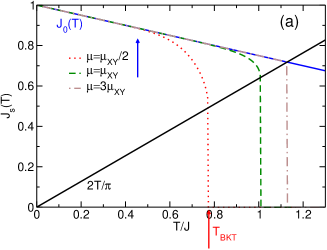
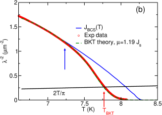
Figure 1: (a) Temperature dependence of the superfluid density for different values of the ratio $\mu/J$, measured in units of the value (17) it has within the XY model. Notice that for small $\mu$ values the deviation from $J_{0}(T)$ starts much before (blue arrow) than the temperature where the universal jump (red arrow) occurs. This behavior is indeed observed in thin NbN films, panel (b). Here we report data from Ref. [pratap_bkt_prl11, ] along with the theoretical BKT fit. Notice that the jump here is further smeared out by the inhomogeneity, see Sec. IV below.

It must be emphasized that the case of thin NbN films must be seen as a paradigmatic example of manifestation of the universal relation (35), despite the fact that $T_{BKT}$ is lower than expected for a standard view based on the $XY$-model results. Indeed, in this system once that the renormalized stiffness is of the order of $2T/\pi$ the transition actually occurs. A different behavior is instead observed in the case we discussed recentlybenfatto_kt_rhos within the context of cuprate superconductors, that can be well modeled as weakly coupled 2D layers. In this case, an additional energy scale exists, i.e. the Josephson coupling $J_{c}$ between layers, which is also a relevant coupling under RG flow, so that a vortex-core energy different from the $XY$-model value can lead to a qualitatively different behavior. We notice that the case of weakly-coupled layered superconductors has been widely investigated in the past within the framework of a layered version of the $XY$-model (1). In this case the presence of a finite interlayer coupling $J_{c}\ll J$ cuts off the logarithmic divergence of the in-plane vortex potential at scales $\sim a/\sqrt{\eta}$,cataudella where $\eta=J_{c}/J$, so that the superfluid phase persists above $T_{BKT}$, with $T_{c}$ at most few percent larger than $T_{BKT}$. chattopadhyay ; friesen ; pierson As far as the superfluid density is concerned, there is some theoreticalchattopadhyay and numericalminnaghen_mc_xymodel evidence that even for moderate anisotropy the universal jump at $T_{BKT}$ is replaced by a rapid downturn of $\rho_{s}(T)$ at a temperature $T_{d}$ larger than the $T_{BKT}$ of each layer, but still very near to it $T_{d}\simeq T_{KT}$. Once more this result must be seen as an indication that the (only) scale $J$ dominates the problem: the result can be different when $\mu$ is allowed to vary, making the competition with the interlayer coupling more subtle.

The analysis of the more general case has been done in a very convenient way in Ref. benfatto_kt_rhos, within the framework of the sine-Gordon model (21), that must be suitable extended to include the interlayer coupling. As we said, in the sine-Gordon model (21) the variable $\theta$ represents the SC phase. Since the phases in neighboring layers are coupled via a Josephson-coupling like interaction, the most natural assumption is an additional cosine term of strength $J_{c}$ for the interlayer phase difference, which translates in an interchain hopping term in the language of the 1D quantum model. A similar model has been also derived recently in Ref. [nandori_jpcm07, ] by using as the starting point the Lawrence-Doniach model for the layered superconductor. The full Hamiltonian that we consider is:benfatto_kt_rhos

$$H=\sum_{m}H_{sg}[\phi_{m},\theta_{m}]-\frac{v_{s}g_{J_{c}}}{2\pi a^{2}}\sum_{\langle m,m^{\prime}\rangle}\int_{0}^{L}dx\cos[\theta_{m}-\theta_{m^{\prime}}],$$ (36)

where $m$ is the layer (chain) index and $g_{J_{c}}\equiv\pi J_{c}/{T}$. In Ref. benfatto_kt_rhos, we derived the perturbative RG equations for the couplings of the model (36) by means of the operator product expansion, in close analogy with the analysis of Ref. [ho_deconfinement_short, ; cazalilla_deconfinement_long, ] for the multichain problem. Under RG flow an additional coupling $g_{\perp}$ between the phase in neighboring layers is generated:

$$\frac{g_{\perp}}{2\pi}\sum_{\langle m,m^{\prime}\rangle}\int dx\left[-K(\partial_{x}\theta_{m})(\partial_{x}\theta_{m^{\prime}})+\frac{1}{K}(\partial_{x}\phi_{m})(\partial_{x}\phi_{m^{\prime}})\right],$$ (37)

which contributes to the superfluid stiffness $K_{s}$, defined as usual as the second-order derivative of the free energy with respect an infinitesimal twist $\delta$ of the phase, $\partial_{x}\theta_{m}\rightarrow\partial_{x}\theta_{m}-\delta$. Thus, one immediately sees that Eq. (37) represents an interlayer current-current term, which contributes to the in-plane stiffness $J_{s}$ as:

$$K_{s}=K-nKg_{\perp},\quad J_{s}=\frac{K_{s}(\ell\rightarrow\infty)T}{\pi},$$ (38)

where $n=2$ corresponds to the number of nearest-neighbors layers. The full set of RG equations for the couplings $K,K_{s},g_{u},g_{J_{c}}$ reads:

$$\frac{dK}{d\ell} = 2g_{J}^{2}-K^{2}g_{u}^{2},$$ (39)

$$\frac{dg_{u}}{d\ell} = (2-K)g_{u},$$ (40)

$$\frac{dK_{s}}{d\ell} = -g_{u}^{2}K_{s}^{2},$$ (41)

$$\frac{dg_{J_{c}}}{d\ell} = \left(2-\frac{1}{4K}-\frac{K_{s}}{4K^{2}}\right)g_{J_{c}}.$$ (42)

Observe that for $g_{J_{c}}=0$ the first two equations reduce to the standard ones (28)-(29) of the BKT transition, and $K_{s}$ coincides with $K$. Instead, as an initial value $g_{J_{c}}\neq 0$ is considered, the interlayer coupling increases under RG,chattopadhyay ; friesen ; pierson contributing to stabilize the $K$ parameter in Eq. (39), with a consequent slowing down of the increase of the $g_{u}$ coupling in Eq. (40). As in the pure 2D case, in the regime where $K$ goes to zero $g_{u}$ increases, see Eq. (40), and vortices proliferate. However, in contrast to the single-layer case where $g_{u}$ becomes always relevant near $K\simeq 2$, here thanks to the $g_{J_{c}}$ term in Eq. (39), $K$ can become smaller than 2 before than $g_{u}$ starts to increase. Since $K_{s}$ is controlled by the $g_{u}$ coupling alone, this means that the system remains superfluid in a range of temperature above $T_{BKT}$ that depends on the competition between vortices ($g_{u}$) and interlayer coupling ($g_{J_{c}}$).

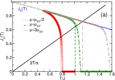
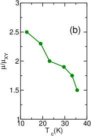
Figure 2: (a) Temperature dependence of the superfluid stiffness $J_{s}(T)$ in the layered 3D case (symbols), taken from Ref. [benfatto_kt_rhos, ]. Here $J_{0}(T)=J(1-T/4J)$ (solid line) mimics the effect of longitudinal excitations within the $XY$ model. It is also shown for comparison the 2D case (lines), see Fig. 1. For $\mu\leq\mu_{XY}$ $J_{s}(T)=0$ at $T_{d}\simeq T_{BKT}$. As $\mu$ increases $T_{d}$ increases as well, so that at $T_{BKT}$ no signature is observed in $J_{s}(T)$ of the jump present in the 2D case. (b) Vortex-core energy in units of $\mu_{XY}$ as a function of the critical temperature of several YBa₂Cu₃O_6+x samples, as derived in Ref. [benfatto_kt_bilayer, ].

The resulting temperature dependence of the superfluid stiffness $J_{s}$ for different values of the vortex-core energy is reported in Fig. 2a, where we added for the sake of completeness a temperature dependence of the bare coupling $J_{0}(T)=J(1-T/4J)$, which mimics the effect of long-wavelength phase fluctuations in the $XY$ model (1). Here the lines represent the pure 2D case (already shown in Fig. 1a above), while the symbols are the result of the RG equations (32)-(42) for a fixed value $J_{c}/J=10^{-4}$ of the interlayer coupling. As one can see, as soon as a finite interlayer coupling is switched on, the jump of $J_{s}(T)$ at $T_{BKT}$ disappears and it is replaced by a rapid bending of $J_{s}(T)$ at some temperature $T_{d}$. However, while for $\mu\leq\mu_{XY}$ $T_{d}$ coincides essentially with $T_{KT}$, for a larger vortex-core energy $T_{d}$ rapidly increases and deviates significantly from the temperature scale where $J_{s}(T)$ intersects the universal line $2T/\pi$.

These results offer a possible interpretation of the measurements of superfluid density reported in strongly-underdoped samples of YBa₂Cu₃O_6+xbroun_prl07 . These systems are exactly the ones where a BKT behavior could be expected: they have a very low in-plane superfluid density and a large ($\eta\sim 10^{-4}$ ) anisotropy of the coupling constants. However, the measured $J_{s}(T)$ goes smoothly across the $T_{BKT}$ estimated from the 2D relation (35). In view of the above discussion, such a behavior does not automatically rules out the possibility that any BKT physics is at play: indeed, if the vortex-core energy is larger than in the $XY$ model the transition can move away from the universal 2D case. Moreover, the effect of inhomogeneity can further round off the downturn induced by vortex proliferation (see next section), making it hardly visible in the experiments. In analogy with the case of conventional superconductors discussed above, a hint on the realistic value of the vortex-core energy in cuprate systems can be inferred by the direct comparison between superfluid-density measurements and the theoretical prediction. We carried out such an analysis in the case of bilayer films of underdoped YBCOlemberger_bilayer for several doping values, showing that $\mu$ attains always values larger than in the $XY$ model, with $1.5<\mu/\mu_{XY}<3$, see Fig. 2b. Moreover, both $\mu$ and the inhomogeneity increase as the system gets underdoped, supporting further the interpretation that a similar effect can be at play also in the data of Ref. [broun_prl07, ]. Interestingly, a very similar trend has been reported recently in NbN systems as disorder increasespratap_bkt_prl11 , and it has been interpreted by the authors as an effect of the increasing separation between the energy scales associated to local pairing and superfluid stiffness as disorder increases. These results suggest that also disorder and inhomogeneity play a crucial role in the understanding of the BKT transition, as we shall discuss in the next section.

IV Inhomogeneity

As we mentioned in the introduction, detailed measurements of superfluid density in thin films of superconductors became available only recently thanks to the efficient implementation of the two-coils mutual inductance technique, which gives access to the absolute value of the penetration depth of thin SC materials. Quite interestingly, in all the cases reported so far in the literature, concerning both conventional superconductorspratap_apl10 ; pratap_bkt_prl11 and high-temperature superconductorsmartinoli_films ; lemberger_bilayer ; bozovic_science09 ; armitage_natphys11 ; lemberger_Bifilms_cm11 the BKT transition is never really sharp. At first sight one could wonder if any finite-size effect is at play, as due to several factors: (i) the existence of a finite screening length $\Lambda\simeq 2\lambda^{2}/d$ due to the supercurrents in a charged superfluidpearl ; (ii) the finite dimension of the system or (iii) the finite length $r_{\omega}$ intrinsically associated to the probe, which uses an ac field at a typical frequency $\omega$ of the order of the KHz. In all the above cases one should cut-off the RG equations (32)-(33) at a finite scale $\ell_{max}=\ln L_{max}/a_{0}$, leading to a rounding of the abrupt jump of the stiffness at $T_{BKT}$. However, in practice such rounding effects are hardly visible, since the decrease of $K(\ell)$ at $T>T_{BKT}$ is very fast, leading to visible rounding effect only for very short cut-off length scales of order of $\ell\simeq 2-3$. In real systems the cut-off length scales are usually much larger: for example, both in the case of the NbN films of Ref. [pratap_apl10, ] and in the case of thin YBCO films from Ref. [lemberger_bilayer, ] $1/\lambda^{2}$ is or order of about 1 $\mu$m^-2 near the transition and $d$ is of the order of 1 nm, so that the Pearl length $\Lambda$ is of the order of 1mm, i.e. comparable to the system size, leading to $\ell_{max}$ around $10$ ($a_{o}$ is of the order of the coherence length $\xi_{0}\sim 1$ nm), which is practically an infinite cut-off for the RG. At the same time $r_{\omega}=\sqrt{14D/\omega}$ is the maximum length probed by the oscillating field, where $D\sim\hbar/m=10^{16}$ Ų/s is the diffusion constant of vortices and $\omega\simeq 50$ KHz is the frequency of the measurementslemberger_bilayer ; pratap_apl10 , giving again a large cut-off scale $r_{\omega}\sim 0.1$ mm and no visible rounding effect, see Fig. 3a. It is worth noting that in the case of the experiments of Ref. lemberger_bilayer, a second indication of the existence of pronounced rounding effects come from the experimental observation of a wide peak in the imaginary part of the conductivity around $T_{BKT}$. Following the dynamical BKT theory of Ambegaokar et al.ambegaokar_fin_freq and Halperin and Nelsonhalperin_ktfilms such a peak is due to the bound- and free-vortex excitations contribution to the complex dielectric constant $\varepsilon(\omega)=\varepsilon^{1}+i\varepsilon^{2}$ which appears in the complex conductivity $\sigma=\sigma_{1}+i\sigma_{2}$ at a finite frequency $\omega$:

$$\sigma(\omega)=-\frac{1}{\lambda^{2}e^{2}\mu_{0}}\frac{1}{i\omega\varepsilon(\omega)}.$$ (43)

Here $\mu_{0}$ is the vacuum permettivity and we used MKS units as in Ref.s [benfatto_kt_bilayer, ; lemberger_bilayer, ]. As in the case of the superfluid-density jump, we estimatedbenfatto_kt_bilayer the width $\Delta T_{\omega}$ in $\sigma_{1}(\omega)$ due to the finite frequency $\omega$ of the measurements and we showed that it is expected to be much smaller than the experimental observations in Ref. lemberger_bilayer, , see Fig. 3a.

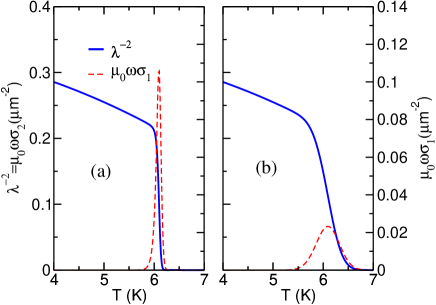
Figure 3: Role of inhomogeneity, from Ref. [benfatto_kt_bilayer, ]. (a) $1/\lambda^{2}$ and $\mu_{0}\omega\sigma_{1}$ evaluated at $\omega=50$ KHz for a single $\bar{J}(T)$ curve using parameter values appropriate for YBa₂Cu₃O_6+x films from Ref. [lemberger_bilayer, ]. Here $\mu=3\mu_{XY}$. The finite frequency leads to a sharp but continuous decrease of $1/\lambda^{2}$ across $T_{BKT}$, along with a peak in $\sigma_{1}$. (b) $1/\lambda^{2}$ and $\mu_{0}\omega\sigma_{1}$ evaluated at finite frequency taking into account the presence of inhomogeneities, as explained in the text.

On the light of the above discussion, we proposed in Ref. benfatto_kt_bilayer, that a more reasonable explanation for the rounding effects in the superfluid density and the large transient region in $\sigma_{1}(\omega)$ observed in the experiments is the sample inhomogeneity. In the case of cuprate systems such inhomogeneity is suggested by tunneling measurements in other families of cuprates,yazdani_07 where Gaussian-like fluctuations of the local gap value are observed. Recently similar local-gap distributions have been reported also in tunneling experiments in thin films of strongly-disordered conventional superconductorssacepe_stm_prl08 ; sacepe_stm_natcom10 ; sacepe_stm_natphys11 ; pratap_prl11 ; pratap_stm_cm11 , showing that an intrinsic tendency towards mesoscopic inhomogeneity appears even for systems with homogeneous intrinsic disorder. Even though the issue of the microscopic origin of this effect is beyond the scope of our work, nonetheless we found that a Gaussian-like distribution of the superfluid-stiffness $J_{0}$ values around a given $\bar{J}$ can account very well for the data of Ref. [lemberger_bilayer, ] on two-unit-cell thick films of YBa₂Cu₃O_6+x. Thus, we compared with the experiments the quantity $J_{inh}(T)=\int dJ_{0}P(J_{0})J(T,J_{0})$, where each $J(T,J_{0})$ curve is obtained from the 2D RG equations using a bare superfluid stiffness $J=J_{0}-\alpha T^{2}$. Each initial value $J_{0}$ has a probability $P(J_{0})=\exp[-(J_{0}-\bar{J}_{0})^{2}/2\sigma^{2}]/(\sqrt{2\pi}\sigma)$ of being realized, where the bare average stiffness follows the typical temperature dependence due to quasiparticle excitations in a (disordered) $d$-wave superconductor, i.e. $\bar{J}(T)=\bar{J}_{0}-\alpha T^{2}$, with $\bar{J}_{0}$ and $\alpha$ fixed by the experimental data at low $T$, where $J_{exp}(T)$ is practically the same as $\bar{J}(T)$. Using a variance $\sigma=0.05\bar{J}_{0}$ we obtained a very good agreement with the experiments near the transition, as far as both both the tail of $\lambda^{-2}$ and the position and width of $\sigma_{1}(\omega)$ are concerned, see Fig. 3b.

Even though our approach to the issue of inhomogeneity is quite phenomenological, it has been shown more recently that it accounts very well also for the superfluid-density behavior in films on NbNpratap_apl10 ; pratap_bkt_prl11 . In all these cases indeed the rounding effect due to inhomogeneity is far more relevant than any finite-size effect due to screening or finite-frequency probes, explaining the lack of a very sharp jump even for relatively weakly-disordered films (see Fig. 1(b) above). Quite interestingly a similar physical picture seems to be relevant also for a completely different class of materials, i.e. the SC metal-oxides interfaces, where experimental data for the superfluid density are not yet available, but the nature of the SC transition can be investigated in an indirect way by means of the analysis of the paraconductivity above $T_{BKT}$triscone_science07 . For these systems as well a BKT transition is likely to be expected, since the SC interfaces are very thintriscone_science07 , of the order of 15 nm, which is much lower than the SC coherence length $\xi_{0}\simeq 70$ nm. Moreover, despite what occurs in thin films of conventional superconductorspratap_bkt_prl11 , the drop of the resistivity above the transition is very smooth, suggesting that inhomogeneities on a mesoscopic scale broaden considerably the transition, as we discussed in details in Ref. [benfatto_kt_interfaces, ]. On this respect, it is worth recalling that any analysis of the BKT transition based on the paraconductivity data alone can suffer of the unavoidable lack of knowledge about the exact extension of the BKT fluctuation regime. Indeed, as we mentioned in the introduction, the contribution of SC fluctuations to the paraconductivity is encoded in the temperature dependence of the correlation length $\xi(T)$ both within the BKT and GL theory, see Eq. (4). Thus, if the transition has BKT character, one should expect a crossover from the BKT exponential temperature dependence of $\xi(T)$,

$$\xi_{BKT}=A\exp(b/\sqrt{t}),\quad t\equiv\frac{T-T_{BKT}}{T_{BKT}},$$ (44)

to the power-law GL one, $\xi_{GL}\sim\xi_{0}T_{c}/(T-T_{c})$, where $T_{c}$ is the BCS mean-field critical temperature. In the case of thin films of superconductors the BKT regime is in practice restricted to a very small range of temperatures near $T_{BKT}$, due to the fact that $T_{c}$ at most twenty per cent larger than $T_{BKT}$. In the case of the SC interfaces it has been proposed instead in the recent literaturetriscone_science07 ; triscone_nature08 ; schneider_finitesize09 that $T_{c}$ is far larger than $T_{BKT}$, so that the whole fluctuation regime above $T_{BKT}$ is dominated by BKT fluctuations alone, while the large tails observed experimentally near $T_{BKT}$ should be ascribed to finite-size effects, see Fig. 4a. There is however a serious drawback in such interpretation, that originates from an incorrect application of the BKT relation (44) in the analysis of the experimental data. As we showed in details in Ref. [benfatto_kt_interfaces, ] by means of a RG analysis of the correlation length, the parameter $b$ which appears in the usual BKT formula (44) is directly connected to the distance $t_{c}=(T_{c}-T_{BKT})/T_{BKT}$ between the mean-field $T_{c}$ and the BKT transition temperature and to the value of the vortex-core energy with respect to the superfluid stiffness:

$$b_{theo}\sim\frac{4}{\pi^{2}}\frac{\mu}{J_{s}}\sqrt{t_{c}},\quad t_{c}=\frac{T_{c}-T_{BKT}}{T_{BKT}}.$$ (45)

As a consequence, $b$ increases when the BKT fluctuation regime extends in temperature. In the typical fits of the resistivity proposed in Ref. triscone_nature08 ; schneider_finitesize09 one obtains values of the $b$ parameter that, according to Eq. (45) above, would imply a mean-field $T_{c}$ very near to $T_{BKT}$, see for instance Fig. 4a. In other words, the fit leads to values of $b$ that contradict the a-priori assumption that the whole fluctuations regime is dominated by BKT fluctuation, as described by Eq. (44). Moreover, also the interpretation of the tails extending below $T_{BKT}$ as due to finite-size effectsschneider_finitesize09 leads to unphysical low values for the size of the homogeneous domains.benfatto_kt_interfaces One would have thus to invoque a BKT transition of a completely differente nature (dislocations of a vortex crystalgabay_melting ), as it has been suggested in Ref. [triscone_science07, ]. However, even in this case there is no theoretical understanding how to reconcile such contradictory numbers obtained in the analysis of the resistive transition.

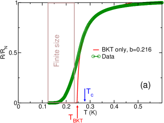
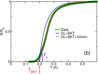
Figure 4: Analysis of the paraconductivity effect on the resistivity of SC interfaces at the $T_{BKT}$ transition. The experimental data for the resistivity $R$ normalized to the normal-state value $R_{N}$ are taken from Ref. [triscone_nature08, ]. Panel (a) shows an example of the approach proposed in [triscone_science07, ; triscone_nature08, ; schneider_finitesize09, ], where the whole range of temperatures above $T_{BKT}$ is dominated by SC fluctuations having BKT character, and finite-size effects are responsible for the resistive tail below $T_{BKT}$. However, the $b$ value obtained by the BKT fit based on Eq. (44) for the correlation length implies, according to Eq. (45), the $T_{c}$ value marked by the blue arrow, invalidating thus the assumption itself that the whole fluctuation regime has BKT character. Panel (b) is taken from Ref. caprara_prb11, (Fig. 5.1 in that paper) and elucidates the approach developed in Refs. benfatto_kt_interfaces, ; caprara_prb11, , based on the interpolation scheme (46) between BKT and GL fluctuation. The curve labeled “GL+BKT+inhom” has been computed by solving a random-resistor network problem with a Gaussian distribution ($\sigma=0.035$ K) of the critical temperatures centered around $\bar{T}_{BKT}=0.2$ K, marked by an arrow along with the corresponding $\bar{T}_{c}=0.22$ K. The paraconductivity of each resistor follows Eq. (46) with $b=0.25$, which according to Eq. (45) corresponds to $t_{c}=0.1$ when $\mu/J_{s}\simeq 2$, an intermediate value between the $XY$ model (17) and BCS (31) estimates. The curve labeled “GL+BKT” corresponds to the homogeneous case with a transition temperature $\bar{T}_{BKT}$.

An alternative, and less far fetched, interpretation of the resistivity data can be based instead on the use of the interpolation formula for $\xi(T)$ proposed long ago by Halperin and Nelsonhalperin_ktfilms

$$\frac{R}{R_{N}}=\frac{1}{1+(\xi/\xi_{0})^{2}},\quad\xi(T)=\xi_{0}A\sinh\frac{b}{\sqrt{t}}.$$ (46)

One can easily see that Eq. (46) reduces to $\xi_{BKT}$ for small $t$ and to $\xi_{GL}$ for large $t$. Using the estimate (45) for the $b$ parameter one realizes that the crossover occurs around $t\simeq b^{2}\propto t_{c}$, so that for (realistic) small values of $t_{c}$ most of the fluctuation regime is dominated by GL-type fluctuations. Moreover, we attributed the broadening of the transition to the effect of inhomogeneity, that induces a distribution of possible realizations of local $R/R_{N}$ values corresponding to the local $J$ values discussed above. An example is shown in Fig. 4b, where the average resistivity has been computed by solving a random-resistor-network model for a set of resistors undergoing a metal-superconductor transition, as discussed recently in Ref. [caprara_prb11, ]. It must be emphasized that the issue of the physical value of the $b$ parameter in the BKT expression (44) of the correlation length has been often overlooked in the literature also in contexts of other materialstriscone_fieldeffect ; iwasa_natmat10 , leading to questionable conclusions concerning the existence of a BKT physics based only on erroneous fits of the resistivity. In contrast, a recent analysis on NbN filmspratap_bkt_prl11 , based on the comparison between the estimate of $b$ deduced from the analysis of the superfluid density below $T_{BKT}$ and the resistivity above $T_{BKT}$ has confirmed the theoretical estimate (45) of the $b$ parameter, that must be used as an unavoidable constraint in any BKT fit of the paraconductivity.

V The case of a finite magnetic field

As we discussed in the previous Sections, the sine-Gordon model provided us with the most appropriate formalism to investigate not only the role of a vortex-core energy value different from the $XY$-model one, but also the occurrence of BKT physics in the presence of a relevant perturbation (in the RG sense), as the interlayer coupling. It is then worth asking the question of the possible relevance of such a mapping for an other typical relevant perturbation, i.e. a finite external magnetic field. The nature of the BKT physics in the presence of a magnetic field has been of course already investigated in the pastreview_minnaghen ; doniach_films ; minnaghen_finitefield , with a renewed interest in the more recent literaturesondhi_kt ; huse_prb08 ; podolsky_prl07 triggered once more by experiments in cuprate superconductors carried out at finite field, as the measurement of the Nerst effect or the magnetization. Unfortunately, contrary to the case of the ${\bf B}=0$ transition, the efforts have been partly unsatisfactory. In particular most of the literature on the subject rested on the use of the mapping into the Coulomb-gas problem, where the effects of the magnetic field can be incorporated as an excess of positive charges, in analogy with the finite population of vortices with a given vorticity due to the presence of the external field. There is however a fundamental drawback of this approach, since it gives the physical observables as a function of the magnetic induction ${\bf B}$ instead of the magnetic field ${\bf H}$. This is of course not convenient at low applied field, since inside the superconductor ${\bf B}$ vanishes even for a finite external field ${\bf H}$. Motivated by this observation and by the occurrence of an anomalous non-linear regime for the magnetization measured in cuprate systems, we showed recentlybenfatto_kt_magnetic that a suitable mapping into the sine-Gordon model provides a very simple and physically transparent way to deal with the finite magnetic-field case, leading to a straightforward definition of the physical observables and clarifying the role of both ${\bf B}$ and ${\bf H}$. Since the construction of the mapping has not been shown in Ref. [benfatto_kt_magnetic, ] due to space limitation, we shall discuss here both the model derivation and its basic physical consequences. This will complete our overview of the sine-Gordon approach to the BKT physics, and it will allow us also to clarify some aspects of the charged superfluid that have not been underlined yet in the previous Sections.

As a starting point we use again the $XY$ model (1), where the coupling to $B$ is introduced via the minimal-coupling prescription for the vector potential ${\bf A}$,

$$H=J\sum_{<i,j>}[1-\cos(\theta_{i}-\theta_{j}-F_{ij})]$$ (47)

where

$$F_{ij}=F_{\mu}(r)=\frac{2\pi}{\Phi_{0}}\int_{r}^{r+\mu}{\bf A}\cdot d{\bf l}\approx\frac{2\pi a}{\Phi_{0}}{\bf A}_{\mu}(r).$$ (48)

Here $\mu=\hat{x},\hat{y}$ is the vector from one site to the neighboring one and $\Phi_{0}=hc/2e$ is the flux quantum. As a first step we make use of the Villain approximation, that amounts to replace the cosine in Eq. (47) with a function having the same minima for each multiple $2\pi m$ of the gauge-invariant phase difference, i.e.

$$\exp[-\beta J(1-\cos(\theta_{i}-\theta_{j}-F_{ij})]\Rightarrow\sum_{m=-\infty}^{m=\infty}\exp\left[-\frac{\beta J}{2}(\theta_{i}-\theta_{j}-F_{ij}-2\pi m)^{2}\right].$$ (49)

By following the analogous derivation given in Ref. [nagaosa_book, ] for the case ${\bf A}=0$, we make use of the Poisson summation formula

$$\sum_{m=-\infty}^{m=\infty}h(m)=\sum_{l=-\infty}^{l=\infty}\int dzh(z)e^{2\pi ilz},$$ (50)

and by performing explicitly the integration over $z$ for each link $ij$ we are left with the following structure of the partition function:

$$Z=Z_{J}\sum_{\{l_{ij}\}}\int_{0}^{2\pi}d\theta_{1}...d\theta_{N}e^{-\sum_{<i,j>}\frac{l_{ij}^{2}}{2\beta J}+i\sum_{\langle i,j\rangle}l_{ij}(\theta_{i}-\theta_{j}-F_{ij})},$$ (51)

where $N$ is the number of lattice sites and $l_{ij}$ are $2N$ integer variables defined for each link $ij$. The prefactor $Z_{J}=[(1/\beta J)^{1/2}]^{2N}=(1/\beta J)^{N}$ accounts for the $z$ integration above for each link. Since each $\theta$ variable is defined on a period, we have that $\int_{0}^{2\pi}d\theta e^{i\theta\alpha}=\delta(\alpha)$. As a consequence, the integration over the $\theta_{i}$ variables in the above equation leads to $N$ constraint equations:

$$\sum_{\mu}l_{\mu}({\bf r})-l_{\mu}({\bf r}-\mu)=0,$$ (52)

which are the discrete equivalent of $\nabla\cdot{\bf l}=0$. These equations can be satisfied by defining for each site of the lattice a field $n$ such that:

$$l_{x}({\bf r})=n({\bf r})-n({\bf r}-y),$$ (53)

$$l_{y}({\bf r})=n({\bf r}-x)-n({\bf r}),$$ (54)

i.e. the discrete equivalent of the relation ${\bf l}=\nabla\times(n\hat{z})$. By means of Eqs. (53)-(54) Eq. (51) can be then rewritten as:

$$Z=Z_{J}\sum_{\{n({\bf r})\}}e^{\sum_{{\bf r},\mu}\frac{1}{2\beta J}(\Delta_{\mu}n({\bf r}))^{2}}e^{-i\frac{2\pi a}{\Phi_{0}}\sum_{\bf r}\hat{z}\cdot({\bf A}\times\Delta n)},$$ (55)

where $\Delta_{\mu}=n({\bf r}+\mu)-n({\bf r})$ is the discrete derivative. Finally, we can use again the Poisson summation formula to get:

$$Z=Z_{J}\int{\cal{D}}\phi({\bf r})\sum_{\{m({\bf r})\}}e^{-\sum_{{\bf r},\mu}\frac{1}{2\beta J}(\Delta_{\mu}\phi({\bf r}))^{2}+2\pi i\sum_{\bf r}\phi({\bf r})m({\bf r})-i\frac{2\pi a}{\Phi_{0}}\sum_{\bf r}\hat{z}\cdot({\bf A}\times\Delta\phi)},$$ (56)

where the $m({\bf r})$ variables assume arbitrary positive and negative integer values. Before completing the mapping into the sine-Gordon model we notice that in the above equation the $\phi$ variables can be integrated out exactly. By rewriting the last term in the action as $\sum_{\bf r}\hat{z}\cdot({\bf A}\times\Delta\phi)=\sum_{\bf r}\phi\hat{z}\cdot(\Delta\times{\bf A})=Ba\sum_{\bf r}\phi$ one can easily see that the final result is given by

$$Z=Z_{\parallel}\sum_{\{m({\bf r})\}}e^{-2\pi^{2}\beta J\sum_{{\bf r},{\bf r}^{\prime}}[m({\bf r})-f]U(r-r^{\prime})[m({\bf r}^{\prime})-f]},\quad f=\frac{Ba^{2}}{\Phi_{0}}$$ (57)

Here $Z_{\parallel}=Z_{J}\Pi_{q>0}(\beta J/{\bf q}^{2})\equiv\Pi_{q>0}(1/\beta J{\bf q}^{2})$ is the overall contribution due to the longitudinal excitations. In full analogy with the result of Sec. II, the longitudinal modes decouple from the transverse ones, so their contribution $Z_{\parallel}$ to the partition function can be discarded in what follows. The function $V({\bf r})=\sum_{\bf k}e^{i{\bf k}\cdot{\bf r}}U({\bf k})$ is defined trough the Fourier transform $U^{-1}({\bf k})=(4-2\cos k_{x}-2\cos k_{y})$ of the $\Delta_{\mu}$ operator on the square lattice, i.e.

$$V({\bf r})=\int\frac{d^{2}{\bf k}}{(2\pi)^{2}}\frac{e^{i{\bf k}\cdot{\bf r}}}{[4-2\cos k_{x}-2\cos k_{y}]}.$$ (58)

Eq. (57) generalizes the Coulomb-gas formula (11) above to the case of a finite magnetic field. As we did in Sec. (II), we can separate in $V({\bf r})$ the singular part in ${\bf r}=0$ by defining the regular function $G({\bf r})$, i.e. $V({\bf r})=V(0)+G({\bf r})$. Then one sees that

$$\sum_{{\bf r},{\bf r}^{\prime}}[m({\bf r})-f]V(r-r^{\prime})[m({\bf r}^{\prime})-f]=$$

$$= V(0)\left[\sum_{\bf r}(m({\bf r})-f)\right]^{2}+\sum_{{\bf r},{\bf r}^{\prime}}[m({\bf r})-f]G(r-r^{\prime})[m({\bf r}^{\prime})-f]$$

It then follows that also in this case only neutral configurations have a statistical weight different from zero. However, in the presence of a magnetic field the neutrality condition reads:

$$\sum_{\bf r}(m({\bf r})-f)=N_{v}-\frac{Ba^{2}N}{\phi_{0}}=0$$ (59)

which means that the total flux $N_{v}\Phi_{0}$ carried out by the (unbalanced) vortices equals the total flux $Ba^{2}N$ of the magnetic field across the sample. The definition (58) allows us also to determine the value (17) of the chemical potential $\mu$ in the lattice $XY$ model. Indeed, one can see that at the scale of the lattice spacing $V({\bf r})-V(0)$ gives:

$$V({\bf r}=\hat{x})-V(0) = \int\frac{d^{2}{\bf k}}{(2\pi)^{2}}\frac{\cos k_{x}-1}{[4-2\cos k_{x}-2\cos k_{y}]}=$$ (60)

$$= \frac{1}{2}\int\frac{d^{2}{\bf k}}{(2\pi)^{2}}\frac{\cos k_{x}+\cos k_{y}-2}{[4-2\cos k_{x}-2\cos k_{y}]}=-\frac{1}{4},$$

so that from Eq. (57) it follows that the cost to put two vortices at distance $a$ apart is $\beta\mu=\beta\pi^{2}J/2$, consistent with the value (17) that we quoted above.

Let us now go back to the Eq. (56) and let us complete the mapping into the sine-Gordon model. We notice that in Eq. (56) the variable $\phi$ is still defined on the square lattice. We can however resort to a continuum approximation by taking into account the energetic cost $\mu$ of the vortex creation on the shortest length scale of the problem via a chemical-potential like term $e^{\ln y\sum_{\bf r}m^{2}({\bf r})}$ in Eq. (56):

$$Z=\int{\cal{D}}\phi({\bf r})\sum_{\{m({\bf r})\}}e^{-\sum_{{\bf r},\mu}\frac{1}{2\beta J}(\Delta_{\mu}\phi({\bf r}))^{2}+2\pi i\sum_{\bf r}\phi({\bf r})m({\bf r})-i\frac{2\pi a}{\Phi_{0}}\sum_{\bf r}\hat{z}\cdot({\bf A}\times\Delta\phi)}e^{\ln y\sum_{\bf r}m^{2}({\bf r})}$$ (61)

The vortex-core energy term favors the formation of vortices of smallest vorticity, i.e. $m({\bf r})=0,\pm 1$. If we limit ourselves to this case the sum over the integer variables $m({\bf r})$ can be performed explicitly as:

$$\sum_{m({\bf r})=0,\pm 1}e^{\ln ym^{2}+2\pi im\phi}=1+2y\cos(2\pi\phi)\approx e^{2y\cos(2\pi\phi)}$$ (62)

Inserting this into Eq. (56), taking the limit of the continuum $(\sum_{\bf r}\rightarrow(1/a^{2})\int d^{2}{\bf r})$, and rescaling $\phi\rightarrow\phi/\pi$ we finally obtain a partition function expressed in terms of the $\phi$ field only, that generalizes Eq. (23) above:

$$S_{B}=\int d{\bf r}dz\left[\frac{(\nabla\phi)^{2}}{2\pi K}\!-\!\frac{g}{\pi a^{2}}\cos 2\phi+\frac{2i}{\Phi_{0}}{\bf A}\!\cdot\!(\nabla\times\hat{z}\phi)\right]\delta(z),\,$$ (63)

where we used again the definitions (28)-(29) for $K,g$. In Eq. (63) we added also the explicit $z$ dependence of the action, which is needed since the ${\bf A}$ field depends in general also on the $z$ out-of-plane coordinate. The $\delta(z)$ function gives the proper boundary conditions for a truly 2D case (where there is no SC current outside the plane), while in the physical case of a SC film of finite thickness $d$ we shall assume that the sample quantities are averaged over $|z|<d/2$.

The action (63) and its corresponding partition function $Z=\int{\cal{D}}\phi e^{-S_{B}}$ allow for a straightforward definition of the physical observables at finite field. For example, the electrical current follows as usual from the functional derivative of $F=-(1/\beta)\ln Z$ with respect to the gauge field ${\bf A}$, i.e

$${\bf J}_{s}({\bf r},z)=-c\frac{\partial F}{\partial{\bf A}({\bf r},z)}=-\frac{2ick_{B}T}{\Phi_{0}}\langle\nabla\times\hat{z}\phi({\bf r})\rangle\delta(z).$$ (64)

The Eq. (64) makes it evident that the current is purely transverse, as expected for vortex excitations, according to the discussion given in Sec. II above. A second quantity that can be easily obtained is the magnetization ${\bf M}=({\bf B}-{\bf H})/4\pi$, defined as the functional derivative of $F$ with respect to ${\bf B}({\bf r},z)=\nabla\times{\bf A}$. By integrating by part and using the identity $\int({\bf A}\times\nabla\phi)\cdot\hat{z}=\int\nabla\phi\cdot(\hat{z}\times{\bf A})=-\int\phi\nabla\cdot(\hat{z}\times{\bf A})=\int\phi\hat{z}\cdot(\nabla\times{\bf A})$, we can rewrite the last term of Eq. (63) as

$$S_{B}=\int d{\bf r}dz\left[\frac{(\nabla\phi)^{2}}{2\pi K}\!-\!\frac{g}{\pi a^{2}}\cos 2\phi+\frac{2i}{\Phi_{0}}{\bf B}({\bf r},z)\cdot\hat{z}\phi({\bf r})\right]\delta(z),\,$$ (65)

As a consequence the functional derivative with respect to ${\bf B}$ gives immediately

$${\bf M}({\bf r})=-\frac{1}{d}\int dz\frac{\partial F}{\partial{\bf B}({\bf r},z)}=-\hat{z}\frac{2ik_{B}T}{d\Phi_{0}}\left\langle\phi({\bf r})\right\rangle,$$ (66)

and analogously the uniform magnetic susceptibility $\chi=\partial M_{z}/\partial B_{z}$ is:

$$\chi=-(4k_{B}T)/(d\phi_{0}^{2})\int d{\bf r}\left[\langle\phi({\bf r})\phi(0)\rangle-\langle\phi({\bf r})\rangle\langle\phi(0)\rangle\right].$$ (67)

Notice that the total magnetic moment $\cal M$ associated to the current ${\bf J}_{s}$ is ${\cal M}=(1/2c)\int d{\bf r}dz\,({\bf r}\times{\bf J}_{s})$landau_iv . Using the definition (64) of ${\bf J}_{s}$, one can easily verify that ${\cal M}=\int d^{2}{\bf r}dz{\bf M}$, i.e. the magnetization is the density of magnetic moment of the sample, as expectedlandau_iv . Finally, by exploiting the fact that $e^{-\beta\mu}e^{\pm i2\phi}$ is the operator which creates up and down vortices with density $n_{\pm}$ respectively, we have a straightforward definition of the average vortex number $n_{F}=a^{2}(\langle n_{+}\rangle+\langle n_{-}\rangle)$ and of the excess vortex number $n=a^{2}(\langle n_{+}\rangle-\langle n_{-}\rangle)$ per unit cell as a function of $\phi$ as:

$$n_{F}=2e^{-\beta\mu}\langle\cos(2\phi)\rangle,\quad n=2e^{-\beta\mu}\langle\sin(2\phi)\rangle.$$ (68)

In Eq. (66) above the average value of $\phi$ is computed with the action (63), so that the magnetization is given as a function of the magnetic induction ${\bf B}$. However, as we mentioned above, at low external field it would be more convenient to compute ${\bf M}$ as a function of the applied field ${\bf H}$. This can be achieved by using the Gibbs free energy ${\cal{G}}=-k_{B}T\ln Z_{G}$, where the partition function $Z_{G}$ includes also the contribution of the electromagnetic field $Z_{G}=\int{\cal{D}}\phi{\cal{D}}Ae^{-S}$ and:

$$S=S_{B}+\int{d{\bf r}dz}\left\{\frac{(\nabla\times{\bf A})^{2}}{8\pi k_{B}T}-\frac{(\nabla\times{\bf A})\cdot{\bf H}}{4\pi k_{B}T}\right\}.$$ (69)

Before discussing explicitly the case of a finite external field ${\bf H}$ we would like to stress how Eq. (69) gives also a very convenient description of the role of charged supercurrents in a 2D superconductor. Indeed, even when ${\bf H}=0$ the electromagnetic field ${\bf A}$ in Eq. (69) above describes the magnetic field created by the current themselves in a charged superfluid. In this case, since the SC currents live in the plane, also ${\bf A}$ is a two-dimensional vector, so that $\nabla\times{\bf A}=(-\partial_{z}A_{y},\partial_{z}A_{x},\partial_{x}A_{y}-\partial_{y}A_{x})$. Moreover, is we choose the Coulomb (or radial) gauge $\nabla\cdot{\bf A}=0$, we have that in Fourier space $({\bf k}_{\parallel}\times{\bf A})^{2}=k_{\parallel}^{2}{\bf A}^{2}$. We can then rewrite in Fourier space the terms in ${\bf A}$ of Eq. (69) at ${\bf H}=0$ as:

$$\int\frac{d^{3}{\bf k}}{(2\pi)^{3}}\left\{-\frac{2}{\Phi_{0}}\phi({\bf k}_{\parallel})|{\bf k}_{\parallel}\times A({\bf k}_{\parallel},k_{z})|-\frac{(k^{2}_{z}+{\bf k}_{\parallel}^{2})}{8\pi T}{\bf A}^{2}({\bf k}_{\parallel},k_{z})\right\}.$$ (70)

By integrating out ${\bf A}$ at Gaussian level we obtain a $\phi^{2}$ contribution to the action of the form:

$$\int\frac{d^{3}{\bf k}}{(2\pi)^{3}}\frac{8\pi T}{\Phi_{0}^{2}}\frac{{\bf k}_{\parallel}^{2}}{(k^{2}_{z}+{\bf k}_{\parallel}^{2})}|\phi({\bf k}_{\parallel})|^{2}.$$ (71)

Since $\phi$ depends on ${\bf k}_{\parallel}$ only, we can integrate out $k_{z}$ and obtain that the overall Gaussian action for the $\phi$ field reads:

$$S_{G}=\int\frac{d^{2}{\bf k}_{\parallel}}{(2\pi)^{2}}\frac{1}{2\pi K}[k_{\parallel}^{2}+k_{\parallel}\Lambda^{-1}]|\phi({\bf k}_{\parallel})|^{2},$$ (72)

where we defined:

$$\frac{1}{\Lambda}=\frac{8\pi^{2}KT}{\Phi_{0}^{2}}\equiv\frac{d}{2\lambda^{2}}.$$ (73)

The last equality follows from the definitions (28) and (5) of $K=\pi J/T$ and $J=\Phi_{0}^{2}d/16\pi^{3}\lambda^{2}$, respectively, and it allows us to identify $\Lambda$ with the so-called Pearl screening lengthpearl . Indeed, due to the $k_{\parallel}\Lambda^{-1}$ terms in Eq. (72), one sees that the potential between vortices, which according to the above discussion is the Fourier transform of the Gaussian $\phi$ propagator, decays as $e^{-r/\Lambda}$ at scales $r\gg\Lambda$, instead of the usual $\log r$ dependence observed at all length scales in neutral superfluids.

Let us go back now to the case of a finite external field in Eq. (69) and let us integrate again the gauge field ${\bf A}$. Since now it is present an additional term $-(i/4\pi T){\bf A}({\bf k})\cdot({\bf k}\times{\bf H}(-{\bf k}))$ in $S$, one obtains the following contribution to the action:

$$\frac{8\pi T}{k^{2}}\left|\frac{\phi(-{\bf k}_{\parallel})}{\phi_{0}}(\hat{z}\times{\bf k}_{\parallel})+\frac{i}{8\pi T}({\bf k}\times{\bf H}(-{\bf k}))\right|^{2}.$$ (74)

The quadratic term in $\phi$ corresponds to Eq. (71) above, leading to the screening of the vortex potential. The remaining terms can be written as:

$$S_{\phi-H}=\int\frac{d^{3}{\bf k}}{(2\pi)^{3}}\frac{2i}{\Phi_{0}k^{2}}(\hat{z}\times{\bf k}_{\parallel}\phi({\bf k}_{\parallel}))\cdot({\bf k}\times{\bf H}(-{\bf k})),$$ (75)

and

$$S_{H-H}=\int\frac{d^{3}{\bf k}}{(2\pi)^{3}}\frac{1}{8\pi T}\frac{({\bf k}\times{\bf H})^{2}}{k^{2}}.$$ (76)

Using the identity

$$\int\frac{d^{3}{\bf k}}{(2\pi)^{3}}F_{1}({\bf k})F_{2}(-{\bf k})\frac{1}{{\bf k}^{2}}=\int d^{3}{\bf r}d^{3}{\bf r}^{\prime}F_{1}({\bf r})F_{2}({\bf r}^{\prime})\frac{1}{4\pi|{\bf r}-{\bf r}^{\prime}|},$$ (77)

and the Maxwell equation relating the magnetic field ${\bf H}$ to the distribution of the external current ${\bf J}_{ext}$ producing the field itself

$$\nabla\times{\bf H}=\frac{4\pi}{c}{\bf J}_{ext},$$ (78)

one can easily see that Eq.s (75) and Eq. (76) can be written in real space as:

$$S_{\phi-H}=2i\int d^{3}{\bf r}d^{3}{\bf r}^{\prime}\frac{[\hat{z}\times\nabla\phi({\bf r})]\cdot[\nabla^{\prime}\times{\bf H}({\bf r}^{\prime})]}{4\pi|{\bf r}-{\bf r}^{\prime}|},$$ (79)

and

$$S_{H-H}=-\frac{1}{8\pi T}\int d^{3}{\bf r}d^{3}{\bf r}^{\prime}\frac{{\bf J}_{ext}({\bf r})\cdot{\bf J}_{ext}({\bf r}^{\prime})}{4\pi|{\bf r}-{\bf r}^{\prime}|},$$ (80)

respectively. By integration by part Eq. (79) can be rewritten as:

$$S_{\phi-H} = \frac{2i}{c}\int d^{3}{\bf r}d^{3}{\bf r}^{\prime}\frac{[\hat{z}\times\nabla\phi({\bf r})]\cdot{\bf J}_{ext}({\bf r}^{\prime})}{|{\bf r}-{\bf r}^{\prime}|}=$$ (81)

$$= -\frac{2i}{c}\int d^{3}{\bf r}d^{3}{\bf r}^{\prime}\phi({\bf r})\nabla_{\bf r}\cdot\frac{[{\bf J}_{ext}({\bf r}^{\prime})\times\hat{z}]}{|{\bf r}-{\bf r}^{\prime}|}=$$

$$= \frac{2i}{c}\int d^{3}{\bf r}d^{3}{\bf r}^{\prime}\phi({\bf r})\hat{z}\cdot\frac{[{\bf J}_{ext}({\bf r}^{\prime})\times({\bf r}-{\bf r}^{\prime})]}{|{\bf r}-{\bf r}^{\prime}|^{3}}=$$

$$= \frac{2i}{\Phi_{0}}\int d^{3}{\bf r}\phi({\bf r})\hat{z}\cdot{\bf H}^{0}({\bf r}).$$

In the last equality of Eq. (81) we introduced the reference field ${\bf H^{0}}$, which corresponds to the magnetic field generated by the same distribution of currents ${\bf J}_{ext}$ in the vacuum. According to the Laplace formula, ${\bf H}^{0}$ is given exactly by

$${\bf H}^{0}({\bf r})=\frac{1}{c}\int d^{3}{\bf r}^{\prime}\frac{{\bf J}_{ext}({\bf r}^{\prime})\times({\bf r}-{\bf r}^{\prime})}{|{\bf r}-{\bf r}^{\prime}|^{3}},$$ (82)

leading to Eq. (81) above. One can also recognize in the term (80) the magnetic energy density associated to the reference field ${\bf H}^{0}$,

$$S_{H-H}=-\frac{1}{8\pi T}\int d^{3}{\bf r}({\bf H}^{0})^{2}.$$ (83)

Indeed, since ${\bf H}^{0}$ is the field created by the currents ${\bf J}_{ext}$ in the vacuum it satisfies $\nabla\cdot{\bf H}^{0}=0$, so that $({\bf k}\times{\bf H}^{0})^{2}=({\bf H}^{0})^{2}k^{2}$. Thus ${\bf H}^{0}({\bf k})^{2}=(\nabla\times{\bf H}^{0})/k^{2}={\bf J}_{ext}({\bf k})^{2}/k^{2}$ that is the Fourier transform of Eq. (80). In summary, the full sine-Gordon action after integration of the gauge field can be rewritten as:

$$S=\int\frac{d^{2}{\bf k}_{\parallel}}{(2\pi)^{2}}\frac{k_{\parallel}^{2}+k\Lambda^{-1}}{2\pi K}|\phi({\bf k}_{\parallel})|^{2}-\frac{g}{\pi a^{2}}\int d{\bf r}\cos 2\phi$$

$$+\frac{2i}{\Phi_{0}}\int d{\bf r}\,\phi\,\hat{z}\cdot{\bf H}^{0}({\bf r},z=0)-\int d{\bf r}dz\frac{({\bf H}^{0})^{2}}{8\pi k_{B}T}.$$ (84)

Eq. (84) is the desired result to be used to evaluate the physical observable as a function of the reference field ${\bf H}^{0}$. Once more, the sine-Gordon mapping turns out to provide a quite powerful framework for the investigation of the BKT physics of a superconductor embedded in an external field. Indeed, apart from the fact that it includes automatically the screening effect of the supercurrents discussed above, the action (84) expressed in terms of ${\bf H}^{0}$ has two main advantages. First of all, ${\bf H}^{0}$ is the field quoted in the experimental measurements, since what is known a priori are only the generating currents ${\bf J}_{ext}$. Indeed, ${\bf H}^{0}$ does not coincide in general with the real field ${\bf H}$ even outside the sample, since the ${\bf H}$ configuration takes into account also the field exclusion from the SC sample, the so-called demagnetization effects. For simple sample geometries one can include these effects in a demagnetization coefficient $\eta$, and write in general the following relation between ${\bf B}={\bf H}+4\pi{\bf M}$ and ${\bf H}^{0}$ landau_iv :

$$(1-\eta){\bf H}+\eta{\bf B}={\bf H}^{0}\Rightarrow{\bf B}={\bf H}^{0}+4\pi(1-\eta){\bf M}.$$ (85)

In the complete Meissner phase one has ${\bf B}=0$, which implies $-4\pi{\bf M}={\bf H}$. However, from Eq. (85) it follows that ${\bf H}={\bf H}^{0}/(1-\eta)$ so that:

$${\bf M}=-\frac{1}{4\pi}\frac{{\bf H}^{0}}{1-\eta}.$$ (86)

While for a cylinder $\eta=0$ and ${\bf H}={\bf H}^{0}$, for a film of thickness $d$ and transversal dimension $R$ one has that $\eta\sim 1-d/R$, so one expects to find ${\bf M}\sim(R/d){\bf H}^{0}$ below $H_{c1}$, i.e. a much smaller critical field with respect to the same system in the 3D geometryfetter_films ; landau_iv . Since the magnetization $M$ calculated from Eq. (84) is already a function of ${\bf H}^{0}$, it will include automatically all the demagnetization effects and the complications of the thin-film geometry.

These properties have been derived in Ref. [benfatto_kt_magnetic, ], where the magnetization has been computed by means of a variational approximation for the cosine term in the model (84). While we refer the reader to Ref. [benfatto_kt_magnetic, ] for more details concerning these calculations, we would like to mention here one particular result, that is related to the discussion of the previous Sections. It concerns the behavior of the field-induced magnetization above $T_{BKT}$, that is expectedhalperin_ktfilms to be proportional to $H$ with a coefficient depending on the SC correlation length:

$$M=-\frac{k_{B}T}{d\Phi_{0}^{2}}\xi^{2}H.$$ (87)

In full analogy with the paraconductivity discussed in the previous Sections, the functional dependence of the low-field magnetization $M$ on the BKT correlation length $\xi$ in Eq. (87) is the same as in the GL theory. While this result was already known in the literaturehalperin_ktfilms ; sondhi_kt , our calculations based on the model (84) allowed to establish an upper limit $H_{l}$ for the validity of the linear regime (87)

$$\,H\lesssim H_{l}=0.1\frac{\Phi_{0}}{\xi^{2}}\sqrt{\frac{T-T_{BKT}}{T}}.$$ (88)

Notice that the above relation can be approximately expressed as the condition $\xi\gg\ell_{B}$ for the low-field limit to be applied, where $\ell_{B}^{2}=\Phi_{0}/H$ is the magnetic length scale.lesueur_nerst As $T$ approaches $T_{BKT}$ $\xi$ increases rapidly and the field $H_{l}$ becomes rapidly smaller than the lowest field accessible in the standard experimental set-up. This effect can explain for example the non-linear magnetization effects reported recently in several measurements in cuprate superconductorsli_magn_epl05 ; ong_natphys07 ; li_nerst_prb10 . Indeed, the persistence of a non-linear magnetization up to $H\sim 0.01$ T in a wide range of temperatures above $T_{BKT}$ can be a signature of the rapid decrease of $H_{l}$ as $T\rightarrow T_{BKT}$, which does not contradict but eventually support the BKT nature of the SC fluctuations in these systems. Moreover, since $\xi$ increases as $\mu$ increases, the extremely low values of $H_{l}$ measured in Ref. li_magn_epl05, suggest a value of $\mu$ larger than $\mu_{XY}$, in agreement with the result discussed in Sec. III based on the analysis of the superfluid density. On the other hand also the existence of inhomogeneities can alter the straightforward manifestation of a linear magnetization above $T_{BKT}$, an issue that has not been explored yet neither in the context of cuprates nor in the case of conventional superconductors. Finally, we would like to mention that even though some theoretical work existssondhi_kt on the RG approach to the BKT transition at finite magnetic field based on the Coulomb-Gas analogy, a full analysis of the more general model (84) is still lacking. Such an approach could eventually improve the estimate (88) of the linear regime, based on a variational calculation that is not expected to capture the correct critical behavior as the transition is approached.

VI Conclusions

It is clear that BKT theory has profoundly changed our understanding of quasi-2D superconductors and given us a tool to tackle such challenging and interesting problems. However, more than 40 years after the original discovery, the occurrence of the BKT transition in several quasi-2D superconducting materials remains partly controversial. One can in general identify two possible sources of discrepancies between theoretical predictions and the current experimental scenario. From one side, the original formulation was based on the paradigmatic case of the $XY$ model, that is only one possible model where the BKT transition occurs. Even though it correctly reproduces the critical behavior of all the systems belonging to the same universality class, quantitative discrepancies away from criticality can be observed in different models. This is the case of the strong superfluid-stiffness renormalization below the transition temperature $T_{BKT}$ in the case of superconducting films of conventional superconductors, where the vortex-core energy attains values significantly different from the $XY$ model prediction. From the other side, emerging new materials and improved experimental techniques offer new scenarios for the occurrence of the BKT transition, which coexists with several other phenomena. An example is provided by the case of cuprate superconductors, that are layered systems formed by strongly-correlated 2D SC layers. In this case, the deviations of the vortex-core energy from the $XY$-model value can eventually lead to a qualitative different behavior of the superfluid-density jump at the transition or to strong non-linear field-induced magnetization effects above $T_{BKT}$. In the present article we reviewed a possible approach to all these issues based on the sine-Gordon model. Even though this is certainly not a new approach for the pure 2D case, in the presence of additional relevant perturbations it provides a very convenient framework to investigate the BKT physics. Indeed, it allows not only to incorporate easily the effects of a vortex-core energy value different from the $XY$ model, but also to describe the coupling to the electromagnetic field in a clear way, giving a straightforward and elegant description of the charged superfluid. Finally, we would like to emphasize once more that a quite interesting issue, that applies equally well to conventional and unconventional superconductors, is posed by the role of the intrinsic sample inhomogeneity. Even though we outlined here a kind of mesoscopic approach to the emergence of spatially inhomogenous SC properties, a more microscopic approach to the effect of disorder on the BKT transition would be required, as suggested by some recent numerical worksmeir_epl10 ; meir_transport_prb11 . The theoretical and experimental investigation of this issue will certainly offer an other perspective on the BKT transition in low-dimensional superconductors.

References

- (1) V. L. Berezinsky, Sov. Phys. JETP. 34, 610, (1972).
- (2) J. M. Kosterlitz and D. J. Thouless, J. Phys. C. 6, 1181, (1973).
- (3) J. M. Kosterlitz, J. Phys. C. 7, 1046, (1974).
- (4) S. Doniach and B. A. Huberman, Phys. Rev. Lett. 42, 1169, (1979).
- (5) B. I. Halperin and D. R. Nelson, J. Low. Temp. Phys. 36, 599, (1979).
- (6) J. Pearl, Appl. Phys. Lett. 5, 65, (1964).
- (7) D. R. Nelson and J. M. Kosterlitz, Phys. Rev. Lett. 39, 1201, (1977).
- (8) P. Minnaghen, Rev. Mod. Phys. 59, 1001, (1987).
- (9) T. Giamarchi, Quantum Physics in One Dimension. (Oxford University Press, Oxford, 2004).
- (10) A. Larkin and A. A. Varlamov, Theory of fluctuations in superconductors. (Oxford University Press, Oxford, 2005).
- (11) S. J. Turneaure, T. R. Lemberger, and J. M. Graybeal, Phys. Rev. B. 63, 174505, (2001).
- (12) A. Rüfenacht, J.-P. Locquet, J. Fompeyrine, D. Caimi, and P. Martinoli, Phys. Rev. Lett. 96, 227002, (2006).
- (13) I. Hetel, T. R. Lemberger, and M. Randeria, Nat. Phys. 3, 700, (2007).
- (14) A. Kamlapure, M. Mondal, M. Chand, A. Mishra, J. Jesudasan, V. Bagwe, L. Benfatto, V. Tripathi, and P. Raychaudhuri, Appl. Phys. Lett. 96, 072509, (2010).
- (15) M. Mondal, S. Kumar, M. Chand, A. Kamlapure, , G. Saraswat, G. Seibold, L. Benfatto, and P. Raychaudhuri, Phys. Rev. Lett. 106, 047001, (2011).
- (16) J. Yong, M. Hinton, A. McCray, M. Randeria, M. Naamneh, A. Kanigel, and T. Lemberger. arXiv:1109.4549, (2011).
- (17) S. J. Turneaure, E. R. Ulm, and T. R. Lemberger, J. Appl. Phys. 79, 4221, (1996).
- (18) R. W. Crane, N. P. Armitage, A. Johansson, G. Sambandamurthy, D. Shahar, and G. Grüner, Phys. Rev. B. 75, 094506, (2007).
- (19) W. Liu, M.Kim, G. Sambandamurthy, and N. Armitage, Phys. Rev. B. 84, 024511, (2011).
- (20) L. S. Bilbro, R.V.Aguilar, G.Logvenov, O.Pelleg, I. Bozović, and N. P. Armitage, Nat. Phys. 7, 298, (2011).
- (21) N. Reyren, S. Thiel, A. D. Caviglia, L. F. Kourkoutis, G. Hammerl, C. Richter, C. W. Schneider, T. Kopp, A.-S. Rüetschi, D. Jaccard, M. Gabay, D. A. Muller, J.-M. Triscone, and J. Mannhart, Science. 317, 1196, (2007).
- (22) A. D. Caviglia, S. Gariglio, N. Reyren, D. Jaccard, T. Schneider, M. Gabay, S. Thiel, G. Hammerl, J. Mannhart, and J.-M. Triscone, Nature (London). 456, 624, (2008).
- (23) J. Biscaras, N. Bergeal, A. Kushwaha, T. Wolf, A. Rastogi, R. Budhani, and J. Lesueur, Nat. Comm. 1, 89, (2010).
- (24) J.T.Ye, S. Inoue, K. Kobayashi, Y. Kasahara, H. T. Yuan, H. Shimotani, and Y. Iwasa, Nature Mater. 9, 125, (2010).
- (25) V. Emery and S. Kivelson, Nature (London). 374, 434, (1995).
- (26) P. A. Lee, N. Nagaosa, and X.-G. Wen, Rev. Mod. Phys. 78, 17, (2006).
- (27) J. Corson, R. Mallozzi, J. Orenstein, J. Eckstein, and J. N. Bozovic, Nature. 398, 221, (1999).
- (28) D. Matthey, N. Reyren, T. Schneider, and J.-M. Triscone, Phys. Rev. Lett. 98, 057002, (2007).
- (29) O. Yuli, I. Asulin, O.Millo, D. Orgad, L.Iomin, and G.Koren, Phys. Rev. Lett. 101, 057005, (2008).
- (30) G. Logvenov, A. Gozar, and I. Bozovic, Science. 326, 699, (2009).
- (31) T. Schneider, A. Caviglia, S. Gariglio, N. Reyren, and J.-M. Triscone, Phys. Rev. B. 79, 184502, (2009).
- (32) L. Benfatto, C. Castellani, and T. Giamarchi, Phys. Rev. B. 80, 214506, (2009).
- (33) Y. Wang, L. Li, and N. P. Ong, Phys. Rev. B. 73, 024510, (2006).
- (34) L. Li, J. G. Checkelsky, S. Komiya, Y. Ando, and N. P. Ong, Nat. Phys. 3, 311, (2007).
- (35) L. Li, Y. Wang, S. Komiya, S. Ono, Y. A. G. D. Gu, and N. P. Ong, Phys. Rev. B. 81, 054510, (2010).
- (36) L. Li, Y. Wang, M. J. Naughton, S. Ono, Y. Ando, and N. P. Ong, Europhys. Lett. 72, 451, (2005).
- (37) E. Bernardi, A. Lascialfari, A. Rigamonti, L. Romanò, M. Scavini, and C. Oliva, Phys. Rev. B. 81, 064502, (2010).
- (38) D. A. H. V. Oganesyan and S. L. Sondhi, Phys. Rev. B. 73, 094503, (2006).
- (39) S. Raghu, D. Podolsky, A. Vishwanath, and D. A. Huse, Phys. Rev. B. 78, 184520, (2008).
- (40) D. Podolsky, S. Raghu, and A. Vishwanath, Phys. Rev. Lett. 99, 117004, (2007).
- (41) O. Cyr-Choinière, R. Daou, F. Laliberté, D. LeBoeuf, N. Doiron-Leyraud, J. C. J.-Q. Yan, J.-G. Cheng, J.-S. Zhou, J. B. Goodenough, S. Pyon, T. Takayama, H. Takagi, Y. Tanaka, and L. Taillefer, Nature (London). 458, 743, (2009).
- (42) A. Levchenko, M. R. Norman, and A. A. Varlamov, Phys. Rev. B. 83, 020506, (2011).
- (43) A. Pourret, H. Aubin, J. Lesueur, C. A. Marrache-Kikuchi, L. Berge, L. Dumoulin, and K. Behnia, Nat. Phys. 2, 683, (2006).
- (44) B. Leridon, J. Vanacken, T. Wambecq, and V. V. Moshchalkov, Phys. Rev. B. 76, 012503, (2007).
- (45) F. Rullier-Albenque, H. Alloul, and G. Rikken, Phys. Rev. B. 84, 014522, (2011).
- (46) D. M. Broun, W. A. Huttema, P. J. Turner, S. Ozcan, B. Morgan, R. Liang, W. N. Hardy, , and D. A. Bonn, Phys. Rev. Lett. 99, 237003, (2007).
- (47) B. Sacépé, C. Chapelier, T. I. Baturina, V. M. Vinokur, M. R. Baklanov, and M. Sanquer, Phys. Rev. Lett. 101, 157006, (2008).
- (48) B. Sacépé, C. Chapelier, T. I. Baturina, V. M. Vinokur, M. R. Baklanov, and M. Sanquer, Nature Communications. 1, 140, (2010).
- (49) B. Sacépé, T. Dubouchet, C. Chapelier, M. Sanquer, M. Ovadia, D. Shahar, M. Feigel’man, and L. Ioffe, Nature Phys. 7, 239, (2011).
- (50) M. Mondal, A. Kamlapure, M. Chand, G. Saraswat, S. Kumar, J. Jesudasan, L. Benfatto, V. Tripathi, and P. Raychaudhuri, Phys. Rev. Lett. 106, 047001, (2011).
- (51) M. Chand, G. Saraswat, A. Kamlapure, M. Mondal, S. Kumar, J.Jesudasan, V. Bagwe, L. Benfatto, V. Tripathi, and P.Raychaudhuri. arXiv:1107.0705, (2011).
- (52) K. K. Gomes, A. N. Pasupathy, A. Pushp, S.Ono, Y. Ando, and A. Yazdani, Nature. 447, 569, (2007).
- (53) M. V. Feigel’man, L. B. Ioffe, V. E. Kravtsov, and E. Cuevas, Ann. Phys. 325, 1390, (2010).
- (54) Y. Dubi, Y. Meir, and Y. Avishai, Nature. 449, 876, (2008).
- (55) K. Bouadim, Y. L. Loh, M. Randeria, and N. Trivedi. arXiv:1011.3275, (2011).
- (56) N. Nagaosa, Quantum Field Theory in Condensed Matter Physics. (Springer, New York, 1999).
- (57) D. J. Bishop and J. D. Reppy, Phys. Rev. B. 22, 5171, (1980).
- (58) L. Benfatto, C. Castellani, and T. Giamarchi, Phys. Rev. Lett. 98, 117008, (2007).
- (59) V. Cataudella and P. Minnaghen, Physica C. 166, 442, (1990).
- (60) B. Chattopadhyay and S. R. Shenoy, Phys. Rev. Lett. 72, 400, (1994).
- (61) M. Friesen, Phys. Rev. B. 51, 632, (1995).
- (62) S. W. Pierson, Phys. Rev. B. 51, 6663, (1995).
- (63) P. Minnaghen and P. Olsson, Phys. Rev. B. 44, 4503, (1991).
- (64) I. Nandori, J. Phys. Cond. Matt. 19, 236226, (2007).
- (65) A. F. Ho, M. A. Cazalilla, and T. Giamarchi, Phys. Rev. Lett. 92, 130405, (2004).
- (66) M. A. Cazalilla, A. F. Ho, and T. Giamarchi, New. J. of Phys. 8, 158, (2006).
- (67) L. Benfatto, C. Castellani, and T. Giamarchi, Phys. Rev. B. 77, 100506(R), (2008).
- (68) V. Ambegaokar, B. I. Halperin, D. R. Nelson, and E. D. Siggia, Phys. Rev. B. 21, 1806, (1979).
- (69) M. Gabay and A. Kapitulnik, Phys. Rev. Lett. 71, 2138, (1993).
- (70) S. Caprara, M. Grilli, L. Benfatto, and C. Castellani, prb. 84, 014514, (2011).
- (71) P. Minnaghen, Phys. Rev. B. 23, 5745, (1981).
- (72) L. Benfatto, C. Castellani, and T. Giamarchi, Phys. Rev. Lett. 99, 207002, (2007).
- (73) L. D. Landau and E. M. Lifchitz, Electrodynamics of Continuous Media. (Pergamon, Oxford, 1984).
- (74) A. L. Fetter and P. C. Hohenberg, Phys. Rev. 159, 330, (1967).
- (75) A. Erez and Y. Meir, Europhys. Lett. 91, 47003, (2010).
- (76) G. Y. Conduit and Y. Meir, Phys. Rev. B. 84, 064513, (2011).