Self-similarity and long-time behavior of solutions of the diffusion equation with nonlinear absorption and a boundary source

Abstract

This paper deals with the long-time behavior of solutions of nonlinear reaction-diffusion equations describing formation of morphogen gradients, the concentration fields of molecules acting as spatial regulators of cell differentiation in developing tissues. For the considered class of models, we establish existence of a new type of ultra-singular self-similar solutions. These solutions arise as limits of the solutions of the initial value problem with zero initial data and infinitely strong source at the boundary. We prove existence and uniqueness of such solutions in the suitable weighted energy spaces. Moreover, we prove that the obtained self-similar solutions are the long-time limits of the solutions of the initial value problem with zero initial data and a time-independent boundary source.

Dedicated to Hiroshi Matano on the occasion of his 60th birthday.

1 Introduction

In the studies of reaction-diffusion equations, one canonical problem deals with the following equation [11, 2]:

$$u_{t}=\Delta u-u^{p},\qquad(x,t)\in\mathbb{R}^{d}\times(0,\infty).$$ (1)

Here $p>1$ is a constant and $u=u(x,t)>0$ can be viewed as the concentration of a chemical species diffusing in the $d$-dimensional space subject to degradation whose rate is an increasing function of the species concentration. Usually, one considers the associated Cauchy problem with some non-negative initial data $u(x,0)=u_{0}(x)$. During the 1980’s, this problem attracted a considerable attention, in particular in the case of measure-valued initial data (e.g., when $u_{0}$ is a Dirac mass) [2, 13, 3, 17, 8, 24]. In the course of these studies, it was discovered that (1) possess self-similar solutions for all $1<p<(2+d)/d$, which are smooth for all $t>0$ and converge to zero outside the origin, while blowing up at the origin when $t\to 0^{+}$ [11, 3] (see also [8] for a variational approach). These solutions play important roles in determining the long-time behavior of the solutions of the Cauchy problem for general classes of initial data and in some sense describe the transient dynamics in systems described by (1) [11, 17, 24, 10, 4, 31, 15]. In particular, a special class of self-similar solutions of (1) called very singular solutions attract the physically important class of initial data with sufficiently fast asymptotic decay [17, 9, 11].

Equation (1) with $p\geq 1$ on domains with boundaries also arises as a canonical model of morphogen gradient formation (for recent reviews, see [27, 20, 25, 30]). Morphogen gradients are concentration fields of molecules acting as spatial regulators of cell differentiation in developing tissues [22]. In particular, the case $p>1$ was proposed to describe a robust patterning mechanism whereby morphogen increases the production of molecules which, in turn, increase the rate of morphogen degradation [7]. For example, a protein called Sonic hedgehog (Shh) is known to induce the expression of its receptor Patched, which both transduces the Shh signal and mediates Shh degradation by cells in the Drosophila embryo [5, 16].

An important aspect of morphogen dynamics is the presence of localized sources at the boundary of the morphogenetic field. This leads to the need to consider initial boundary value problems, whose prototype is the following one-dimensional problem:

$$\left\{\begin{array}[]{ll}u_{t}=u_{xx}-u^{p}&(x,t)\in[0,\infty)\times(0,\infty),\\ u_{x}(0,t)=-\alpha&t\in(0,\infty),\\ u(x,0)=0&x\in[0,\infty).\end{array}\right.$$ (5)

This problem can be viewed as an extension of the Cauchy problem for (1) defined for $x>0$ in the presence of a boundary source at $x=0$. Here $\alpha>0$ is a constant characterizing the source strength of morphogen production, and the zero initial condition corresponds to the absence of the morphogen at the onset of patterning. In what follows, we will restrict our attention only to this simplest model of morphogen gradient formation.

In the context of morphogenesis, one is often interested in the establishment of a stationary morphogen profile and the transient dynamics that leads to it. The stationary problem for (5) can be written as the following boundary value problem:

$$v_{xx}-v^{p}=0,\qquad v_{x}(0)=-\alpha,\qquad v(\infty)=0,$$ (6)

whose unique solution for any $p>1$ is explicitly given by

$$v(x)=\left(\frac{2(p+1)}{(p-1)^{2}}\right)^{1\over p-1}(a+x)^{-\frac{2}{p-1}},\quad a=\left(\frac{2^{\frac{p}{p+1}}(p+1)^{\frac{1}{p+1}}}{p-1}\right)\alpha^{-\frac{p-1}{p+1}}.$$ (7)

In fact, it is easy to see that the stationary solution $v(x)$ in (6) is the limit of the solution $u(x,t)$ of (5) as $t\to\infty$ for each $x\geq 0$, and is approached monotonically from below [14]. However, as we noted in [14], this approach is not uniform in $x$ and for each fixed $x\geq 0$ occurs on the diffusive time scale $\tau_{p}(x)=O(x^{2})$, which diverges as $x\to\infty$. Thus, the timing of the establishment of the steady morphogen concentration at a given point depends rather sensitively on the location of that point.

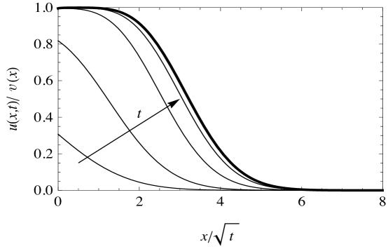
Figure 1: Numerical solution of (5) in self-similar variables for $p=2$ and $\alpha=1$. Thin lines show snapshots of the solution corresponding to $t=0.1,1,10,100$ (the direction of time increase is indicated by the arrow). The bold line shows the asymptotic solution.

To better understand the dynamics of the approach of the solution of (5) to the stationary solution, we undertook numerical studies of the initial boundary problem in (5) for various values of $p>1$. In those studies, we discovered that when the ratio of the solution at a given $x$ to the value of the stationary solution at $x$ is plotted vs. the diffusion similarity variable $x/\sqrt{t}$, the numerical solution approaches some universal limit curve depending only on the value of $p$ [23]. This process is illustrated in Fig. 1, where the results are presented for the biophysically important case $p=2$. This observation suggested to us some hidden self-similarity in the behavior of solutions of (5) [1]. A simple scaling argument indicates that the long-time behavior of the solution of (5) for a fixed value of $\alpha>0$ is closely related to the behavior of solutions of (5) at fixed $x>0$ and $t>0$ as $\alpha\to\infty$ [23]. We found numerically that in the limit $\alpha\to\infty$ the solutions of (5) attain a self-similar profile (see the following section for precise definitions) [23]. The purpose of this paper is to substantiate these numerical observations by establishing existence and properties of what we will call ultra-singular self-similar solutions in the limit of infinite boundary source strength. We also prove that these solutions are indeed the long-time limits of the solutions of (5) in the above sense.

We note that the solutions constructed by us form a new class of self-similar solutions to (1) in $d=1$. Indeed, our solutions can be trivially extended to the whole real line by a reflection and can be viewed as singular solutions of (1) that blow up at the origin. We point out that these solutions are different from the self-similar solutions studied in [11, 3]. The ultra-singular solutions of (1) constructed by us can be viewed as the more singular counterparts of the very singular solutions of [3] in the following sense: the singularity in the former is concentrated on a half-line ($x=0,t>0$) in the $(x,t)$ plane, while the singularity in the latter occurs only at a single point ($x=0,t=0$). Similarly, our convergence result for the solutions of (5) with $\alpha\in(0,\infty)$ may be viewed as a counterpart of the result of [17], in the sense that in the former case the solution can be viewed as the distributional solution of (1) with an added term $2\alpha\delta(x)$ in the right-hand side, while in the latter case one can think of the solution as the distributional solution of (1) with the term $\alpha\delta(x)\delta(t)$ added to the right-hand side.

Before concluding this section, let us briefly mention a few possible extensions and open problems related to our present work. It would be interesting to understand the role our self-similar solutions play for the singular solutions of the initial value problem associated with (1) for general non-zero initial data. Let us point out that even the basic questions of existence and uniqueness of such singular solutions for the considered parabolic problems in suitable function classes are currently open (see [29] for a very recent related work). Other natural extensions include higher dimensional versions of the considered problem, as well as a proof of global stability of self-similar solutions. These studies are currently ongoing. From the point of view of applications, it is also important to consider solutions of (1) with added time-varying singular sources, for which both the very singular and the ultra-singular solutions may be relevant.

Our paper is organized as follows. In Sec. 2, we introduce a singular version of the initial boundary value problem in (5) and prove existence, uniqueness, monotonicity and limiting behavior of the self-similar solution to this singular problem. Then, in Sec. 3 we prove that the obtained self-similar solutions are the long-time limits of the solutions of (5) in an appropriate sense.

2 Singular solutions and the similarity ansatz

Let us consider (5) with infinite source at the boundary, i.e., the following singular initial boundary value problem:

$$\left\{\begin{array}[]{ll}u_{t}=u_{xx}-u^{p}&(x,t)\in(0,\infty)\times(0,\infty),\\ u(0,t)=\infty,&t\in(0,\infty),\\ u(x,0)=0&x\in(0,\infty).\end{array}\right.$$ (11)

By a solution to (11), we mean a classical solution for all $(x,t)\in(0,\infty)\times(0,\infty)$ decaying sufficiently fast as $x\to+\infty$ for all $t>0$, and continuous up to $t=0$ for all $x>0$. Note that for each $p>1$ this problem possesses a singular stationary solution

$$v_{\infty}(x)=\left(\frac{2(p+1)}{(p-1)^{2}}\right)^{1\over p-1}\left({1\over x}\right)^{2\over p-1},$$ (12)

which is the limit of $v_{\alpha}(x)$ as $\alpha\to\infty$ for each $x>0$.

Consistently with the discussion in the introduction, we now seek solutions of (11) in the form

$$u(x,t)=v_{\infty}(x)\phi(\zeta),\quad\zeta=\ln(x/\sqrt{t}),$$ (13)

for some function $0\leq\phi(\zeta)\leq 1$, which will be referred to as the self-similar profile. Substituting the similarity ansatz from (13) into (11), after some algebra we obtain the following equation for the self-similar profile $\phi$:

$${d^{2}\phi\over d\zeta^{2}}+\left(\frac{e^{2\zeta}}{2}-\frac{p+3}{p-1}\right){d\phi\over d\zeta}+\frac{2(p+1)}{(p-1)^{2}}\phi(1-\phi^{p-1})=0,$$ (14)

which must hold for all $\zeta\in(-\infty,\infty)$, supplemented with the limit behavior

$$\lim_{\zeta\to-\infty}\phi(\zeta)=1,\qquad\lim_{\zeta\to-\infty}{d\phi(\zeta)\over d\zeta}=0,$$ (15)

$$\lim_{\zeta\to+\infty}\phi(\zeta)=0,\qquad\lim_{\zeta\to+\infty}{d\phi(\zeta)\over d\zeta}=0.$$ (16)

Existence and multiplicity of solutions of (14) satisfying (15) and (16) are not at all a priori obvious in view of both the non-linearity and the presence of singular terms in the considered boundary value problem. In [23], we were able to construct such solutions numerically for several values of $p$. Here we establish their existence and uniqueness for all $p>1$ within a natural class of functions.

We will prove existence and uniqueness of solutions of (14) satisfying (15) and (16) in the weighted Sobolev space $H^{1}(\mathbb{R},d\mu)$, which is obtained as the completion of the family of smooth functions with compact support with respect to the Sobolev norm $||.||_{H^{1}(\mathbb{R},d\mu)}$, defined as

$$||w||_{H^{1}(\mathbb{R},d\mu)}^{2}=||w_{\zeta}||_{L^{2}(\mathbb{R},d\mu)}^{2}+||w||_{L^{2}(\mathbb{R},d\mu)}^{2},$$ (17)

where $||w||_{L^{2}(\mathbb{R},d\mu)}^{2}=\int_{\mathbb{R}}w^{2}(\zeta)d\mu(\zeta)$, and the measure $d\mu$ is

$$d\mu(\zeta)=\rho(\zeta)d\zeta,\qquad\rho(\zeta)=\exp\left\{\frac{e^{2\zeta}}{4}-\left(\frac{p+3}{p-1}\right)\zeta\right\}.$$ (18)

Our existence and uniqueness result is given by the following theorem.

Theorem 1.

There exists a unique weak solution $\phi$ of (14), such that $\phi-\eta\in H^{1}(\mathbb{R},d\mu)$, with $\mu$ defined in (18), for every $\eta\in C^{\infty}(\mathbb{R})$, such that $\eta(\zeta)=1$ for all $\zeta\leq 0$ and $\eta(\zeta)=0$ for all $\zeta\geq 1$. Furthermore, $\phi\in C^{\infty}(\mathbb{R})$, satisfies (14) classically and $0<\phi<1$. In addition, $\phi$ is strictly decreasing and satisfies (15) and (16).

Before proceeding to the proof of Theorem 1, let us establish a basic technical lemma needed to deal with the weighted spaces introduced above, which is an extension of [21, Lemma 4.1] for exponentially weighted Sobolev spaces (cf. also [8, Lemma 1.5]).

Lemma 1.

Let $w\in H^{1}(\mathbb{R},d\mu)$. Then there exists $R_{0}>0$ such that

$$\int_{R}^{\infty}w^{2}d\mu\leq\frac{e^{-2R}}{2}\int_{R}^{\infty}\left(\frac{dw}{d\zeta}\right)^{2}d\mu\qquad\qquad\forall R\geq R_{0},$$ (19)

and

$$\rho(R)w^{2}(R)\leq 2e^{-R}\int_{R}^{\infty}\left(\frac{dw}{d\zeta}\right)^{2}d\mu\qquad\qquad\text{for a.e. }R\geq R_{0}.$$ (20)

Moreover, there exists $R_{0}^{\prime}<0$ such that

$$\int_{-\infty}^{R}w^{2}d\mu\leq 8\left(\frac{p-1}{p+3}\right)^{2}\int_{-\infty}^{R}\left(\frac{dw}{d\zeta}\right)^{2}d\mu\qquad\qquad\forall R\leq R_{0}^{\prime},$$ (21)

and

$$\rho(R)w^{2}(R)\leq 8\left(\frac{p-1}{p+3}\right)\int_{-\infty}^{R}\left(\frac{dw}{d\zeta}\right)^{2}d\mu\qquad\qquad\text{for a.e. }R\leq R_{0}^{\prime}.$$ (22)

Proof. Arguing by approximation, observe that by an explicit computation and an application of Cauchy-Schwarz inequality we have

$$\frac{1}{2}\left(w^{2}(R)\rho(R)+\int_{R}^{\infty}\left(\frac{d}{d\zeta}\ln\rho\right)w^{2}d\mu\right)\qquad\qquad\qquad\qquad$$

$$=-\int_{R}^{\infty}w\frac{dw}{d\zeta}d\mu\leq\left(\int_{R}^{\infty}w^{2}d\mu\int_{R}^{\infty}\left(\frac{dw}{d\zeta}\right)^{2}d\mu\right)^{1/2}.$$ (23)

In particular, (18) and (23) yield

$$\left(\frac{e^{2R}}{2}-\frac{p+3}{p-1}\right)^{2}\int_{R}^{\infty}w^{2}d\mu\leq 4\int_{R}^{\infty}\left(\frac{dw}{d\zeta}\right)^{2}d\mu,$$ (24)

which for large enough $R$ implies (19). Next, since ${d\over d\zeta}\ln\rho>0$ for large positive $\zeta$, dropping the second term in the left-hand side of (23) and using (19), we obtain (20).

Similarly, we note that

$$\frac{1}{2}\left(w^{2}(R)\rho(R)-\int_{-\infty}^{R}\left(\frac{d}{d\zeta}\ln\rho\right)w^{2}d\mu\right)\qquad\qquad\qquad\qquad$$

$$=\int_{-\infty}^{R}w\frac{dw}{d\zeta}d\mu\leq\left(\int_{-\infty}^{R}w^{2}d\mu\int_{-\infty}^{R}\left(\frac{dw}{d\zeta}\right)^{2}d\mu\right)^{1/2},$$ (25)

which implies

$$\left(\frac{p+3}{p-1}-\frac{e^{2R}}{2}\right)^{2}\int_{-\infty}^{R}w^{2}d\mu\leq 4\int_{-\infty}^{R}\left(\frac{dw}{d\zeta}\right)^{2}d\mu,$$ (26)

and thus (21) holds for sufficiently large negative $R$. Finally since ${d\over d\zeta}\ln\rho<0$ for large negative $\zeta$, from (25) and (21) we obtain (22). ∎

Proof of Theorem 1. The proof consists of five steps.

Step 1. We first note that (14) is the Euler-Lagrange equation for the energy functional

$${\cal E}[\phi]=\int_{\mathbb{R}}\Biggl{\{}\frac{1}{2}\left({d\phi\over d\zeta}\right)^{2}+{\eta\over p-1}-\frac{\phi^{2}(p+1-2\phi^{p-1})}{(p-1)^{2}}\Biggr{\}}d\mu,$$ (27)

where $\eta(\zeta)$ is as in the statement of the theorem. Indeed, the functional $\mathcal{E}$ in (27) is continuously differentiable in $H^{1}(\mathbb{R},d\mu)$ in the natural admissible class $\mathcal{A}$ defined as:

$$\mathcal{A}:=\{\phi\in H^{1}_{\mathrm{loc}}(\mathbb{R}):\phi-\eta\in H^{1}(\mathbb{R},d\mu),\hskip 2.84526pt0\leq\phi\leq 1\}.$$ (28)

Note that the role of $\eta$ in the definition of $\mathcal{E}$ is to ensure that the integral in (27) converges for all $\phi\in\mathcal{A}$. The precise form of $\eta(\zeta)$ is unimportant. Then it is easy to see that the weak form of (14) in $H^{1}(\mathbb{R},d\mu)$ is precisely the condition that the Fréchet derivative of $\mathcal{E}[\phi]$ is zero.

Step 2. We now establish weak sequential lower-semicontinuity and coercivity of the functional $\mathcal{E}$ in the admissible class $\mathcal{A}$ in the following sense: let $\phi_{k}=\eta+w_{k}$, where $w_{k}\rightharpoonup w$ in $H^{1}(\mathbb{R},d\mu)$. Then 1) $\liminf_{k\to\infty}\mathcal{E}[\phi_{k}]\geq\mathcal{E}[\phi]$, where $\phi=\eta+w$, and 2) if $\mathcal{E}[\phi_{k}]\leq M$ for some $M\in\mathbb{R}$, then $||w_{k}||_{H^{1}(\mathbb{R},d\mu)}\leq M^{\prime}$ for some $M^{\prime}>0$.

Let us introduce the notation $\mathcal{E}[\phi,(a,b)]$ for the integral in (27), in which integration is over all $\zeta\in(a,b)$. Then, using (19) from Lemma 1 we find that for $R\geq 1$

$$\mathcal{E}[\phi_{k},(R,+\infty)]\geq\left(e^{2R}-{p+1\over(p-1)^{2}}\right)\int_{R}^{\infty}w_{k}^{2}d\mu>0.$$ (29)

Similarly, taking into account that the integrand in (27) is non-negative for $\zeta\leq 0$, we have $\mathcal{E}[\phi_{k},(-\infty,-R)]\geq 0$ for every $R\geq 0$. Since $\mathcal{E}[\cdot,(-R,R)]$ is lower-semicontinuous by standard theory [6], we obtain $\mathcal{E}[\phi_{k}]\geq\mathcal{E}[\phi_{k},(-R,R)]$, yielding the first claim by passing to the limit $R\to\infty$.

To prove coercivity, we first note that by (19)

$$\mathcal{E}[\phi_{k},(R,+\infty)]\geq\int_{R}^{\infty}\left\{\frac{1}{2}\left({dw_{k}\over d\zeta}\right)^{2}-{p+1\over(p-1)^{2}}w_{k}^{2}\right\}d\mu$$

$$\geq\frac{1}{4}\int_{R}^{\infty}\left\{\left({dw_{k}\over d\zeta}\right)^{2}+w_{k}^{2}\right\}d\mu,$$ (30)

for large positive $R$. On the other hand, since $p-1-\phi^{2}(p+1-2\phi^{p-1})\geq(p-1)(1-\phi)^{2}$ for all $0\leq\phi\leq 1$, we have

$$\mathcal{E}[\phi_{k},(-\infty,0)]\geq\int_{-\infty}^{0}\left\{\frac{1}{2}\left({dw_{k}\over d\zeta}\right)^{2}+{w_{k}^{2}\over p-1}\right\}d\mu.$$ (31)

Finally, by boundedness of $\phi_{k}$ and $\eta$, we also have

$$\mathcal{E}[\phi_{k},(0,R)]\geq\frac{1}{2}\int_{0}^{R}\left\{\left({dw_{k}\over d\zeta}\right)^{2}+w_{k}^{2}\right\}d\mu-CR,$$ (32)

for some $C>0$ independent of $w_{k}$. So the second claim follows.

Step 3. In view of the lower-semicontinuity and coercivity of $\mathcal{E}$ proved in Step 2, by the direct method of calculus of variations there exists a minimizer $\phi\in\mathcal{A}$ of $\mathcal{E}$. Noting that since the barriers $\phi=0$ and $\phi=1$ solve (14) as well, we also have (see e.g. [19]) that $\phi$ is a weak solution of (14) by continuous differentiability of $\mathcal{E}$ in $H^{1}(\mathbb{R},d\mu)$ noted in Step 1. Furthermore, by standard elliptic regularity theory [12], $\phi\in C^{\infty}(\mathbb{R})$ and is, in fact, a classical solution of (14). Also, by strong maximum principle [12], we have $0<\phi<1$. To show monotonicity, suppose, to the contrary, that $\phi(a)<\phi(b)$ for some $a<b$. Then $\phi(\zeta)$ attains a local minimum for some $\zeta_{0}\in(-\infty,b)$. However, by (14) we have $d^{2}\phi(\zeta_{0})/d\zeta^{2}<0$, giving a contradiction. By the same argument $d\phi/d\zeta=0$ is also impossible for any $\zeta\in\mathbb{R}$. Finally, since $\phi-\eta\in H^{1}(\mathbb{R},d\mu)$, monotonicity implies the first condition in (15) and (16).

Step 4. We now discuss the asymptotic behavior of minimizers obtained in Step 3 as $\zeta\to\pm\infty$ and, in particular, prove the second parts of (15) and (16) and the fact that every solution of (14) belonging to $\mathcal{A}$ has the same asymptotic decay, which will be needed later. Let us first consider the case of $\zeta\to+\infty$. Performing the Liouville transformation by introducing

$$\psi=\phi\sqrt{\rho}\in L^{2}(R,+\infty),$$ (33)

where $\rho$ is defined in (18) and $R\geq 1$ is arbitrary, we rewrite (14) in the form

$${d^{2}\psi\over d\zeta^{2}}=q(\zeta)\psi,\qquad\zeta\geq R.$$ (34)

Here $q(\zeta)=q_{0}(\zeta)+q_{1}(\zeta)$, where

$$q_{0}(\zeta) =\frac{1}{4}\left(\frac{e^{4\zeta}}{4}+\frac{p-5}{p-1}e^{2\zeta}+1\right),$$ (35)

$$q_{1}(\zeta) =\frac{2(p+1)}{(p-1)^{2}}\,\phi^{p-1}(\zeta).$$ (36)

Observe that $q(\zeta)\geq q_{0}(\zeta)\geq\tfrac{1}{4}>0$ for all $\zeta\geq R$, with $R$ sufficiently large positive. Therefore, (34) has two linearly-independent positive solutions $\psi_{1}$ and $\psi_{2}$, such that $\psi_{1}\to 0$ and $\psi_{2}\to\infty$ together with their derivatives as $\zeta\to+\infty$ (see e.g. [28]). In particular, $\psi=C\psi_{1}\in L^{2}(R,+\infty)$ for some $0<C<\infty$, and by direct computation

$${d\phi\over d\zeta}={C\over\sqrt{\rho}}\left({d\psi_{1}\over d\zeta}-\frac{\psi_{1}}{2}{d\over d\zeta}\ln\rho\right)\to 0\qquad\text{as}\quad\zeta\to+\infty.$$ (37)

On the other hand, as follows from (20), we have

$$q_{1}(\zeta)=o(\rho^{1-p\over 2}),$$ (38)

so $q_{1}(\zeta)$ has a super-exponential decay as $\zeta\to+\infty$. Let $\psi_{0}$ be the unique positive solution of (34) with $q=q_{0}$ and $\psi_{0}(R)=1$ which goes to zero as $\zeta\to+\infty$. Then we claim that $\psi_{1}(\zeta)/\psi_{0}(\zeta)\to c$ for some $0<c<\infty$. Indeed, functions $\psi_{1}$ and $\psi_{0}$ satisfy

$${d^{2}\psi_{1}\over d\zeta^{2}}=(q_{0}(\zeta)+q_{1}(\zeta))\psi_{1},\quad{d^{2}\psi_{0}\over d\zeta^{2}}=q_{0}(\zeta)\psi_{0},\qquad\zeta\geq R.$$ (39)

Multiplying the first and the second equation of (39) by $\psi_{0}$ and $\psi_{1}$, respectively, and taking the difference, we obtain

$$\frac{d}{d\zeta}\left(\psi_{0}{d\psi_{1}\over d\zeta}-\psi_{1}{d\psi_{0}\over d\zeta}\right)=q_{1}(\zeta)\psi_{0}\psi_{1}.$$ (40)

Integrating this equation and taking into account that $\psi_{0},\psi_{1}$ and their derivatives vanish as $\zeta\to+\infty$, we have

$$\psi_{0}(\zeta){d\psi_{1}(\zeta)\over d\zeta}-\psi_{1}(\zeta){d\psi_{0}(\zeta)\over d\zeta}=-\int_{\zeta}^{\infty}q_{1}(s)\psi_{0}(s)\psi_{1}(s)ds,$$ (41)

and therefore

$${d\over d\zeta}\ln\left({\psi_{1}\over\psi_{0}}\right)=-\int_{\zeta}^{\infty}q_{1}(s){\psi_{1}(s)\psi_{0}(s)\over\psi_{1}(\zeta)\psi_{0}(\zeta)}ds.$$ (42)

Integrating this equation again, we obtain

$$\ln\left({\psi_{1}(\zeta)\over\psi_{0}(\zeta)}\right)=\ln\left({\psi_{1}(R)\over\psi_{0}(R)}\right)-\int_{R}^{\zeta}\int_{\sigma}^{\infty}q_{1}(s){\psi_{1}(s)\psi_{0}(s)\over\psi_{1}(\sigma)\psi_{0}(\sigma)}dsd\sigma.$$ (43)

In a view of boundedness of functions $\psi_{0}$ and $\psi_{1}$, we have $|\psi_{0}(s)/\psi_{0}(\sigma)|,|\psi_{1}(s)/\psi_{1}(\sigma)|\leq C$ for some $C>0$ and all $s\geq\sigma\geq R$. Moreover, the estimate in (38) gives $|q_{1}(s)|\leq C^{\prime}\exp(-s)$ for some $C^{\prime}>0$ and all $s\in[R,\infty)$. Therefore, the integral in the right-hand side of (43) converges:

$$\int_{R}^{\zeta}\int_{\sigma}^{\infty}\left|q_{1}(s){\psi_{1}(s)\psi_{0}(s)\over\psi_{1}(\sigma)\psi_{0}(\sigma)}\right|dsd\sigma\leq C\int_{R}^{\zeta}\int_{\sigma}^{\infty}e^{-s}dsd\sigma\leq Ce^{-R}<\infty,$$ (44)

which immediately implies that the ratio of $\psi_{0}$ and $\psi_{1}$ approaches a finite non-zero limit as $\zeta\to+\infty$.

We can use a similar treatment to establish the asymptotic behavior of minimizers when $\zeta\to-\infty$. The Liouville transformation

$$\theta=(1-\phi)\sqrt{\rho}\in L^{2}(-\infty,R),$$ (45)

with $\rho$ defined by (18) and arbitrary $R\leq 0$ applied to (14) yields

$${d^{2}\theta\over d\zeta^{2}}=r(\zeta)\theta,\qquad\zeta\leq R.$$ (46)

Here $r(\zeta)=r_{0}(\zeta)+r_{1}(\zeta)$, where

$$r_{0}(\zeta) =\frac{1}{4}\left(\left(\frac{3p+1}{p-1}\right)^{2}+\frac{p-5}{p-1}e^{2\zeta}+\frac{e^{4\zeta}}{4}\right),$$ (47)

$$r_{1}(\zeta) =\frac{2(p+1)}{(p-1)^{2}}\left(\frac{\phi(1-\phi^{p-1})}{1-\phi}+1-p\right).$$ (48)

By direct computation, note that in the limit $\zeta\to-\infty$ we have

$$r_{0}(\zeta)\to\frac{1}{4}\left(\frac{3p+1}{p-1}\right)^{2},\qquad r_{1}(\zeta)\to 0^{-}.$$ (49)

Therefore, $r_{0}(\zeta)\geq r(\zeta)\geq\tfrac{1}{4}>0$ for all $\zeta\leq R$ with $R$ sufficiently large negative, and (46) has two linearly-independent positive solutions $\theta_{1}$ and $\theta_{2}$ such that $\theta_{1}\to 0$ and $\theta_{2}\to\infty$ together with their derivatives as $\zeta\to-\infty$. In particular, $\theta=C\theta_{1}\in L^{2}(-\infty,R)$ for some $0<C<\infty$, and

$${d\phi\over d\zeta}=-{C\over\sqrt{\rho}}\left({d\theta_{1}\over d\zeta}-\frac{\theta_{1}}{2}{d\over d\zeta}\ln\rho\right)\to 0\qquad\text{as}\quad\zeta\to-\infty.$$ (50)

On the other hand, as follows from (22) we have

$$r_{1}(\zeta)=o(\rho^{-1/2}),$$ (51)

so $r_{1}(\zeta)$ has an exponential decay as $\zeta\to-\infty$. Computations practically identical to those presented above show that the ratio of $\theta_{0}$ (the solution of (46) with $r=r_{0}$ which decays as $\zeta\to-\infty$) and $\theta_{1}$ tends to a positive constant as $\zeta\to-\infty$.

Step 5. We now prove uniqueness of the obtained solution, taking advantage of a sort of convexity of $\mathcal{E}$ similar to the one pointed out in [18]. Suppose, to the contrary, that there are two functions $\phi_{1},\phi_{2}\in\mathcal{A}$ which solve (14). Define

$$\phi^{t}:=\sqrt{t\phi_{2}^{2}+(1-t)\phi_{1}^{2}}.$$ (52)

We claim that $\phi^{t}\in\mathcal{A}$ as well. Indeed, in view of the result of Step 4 we have $m<\phi_{1}/\phi_{2}<M$ for some $M>m>0$ and, therefore,

$$||\phi^{t}||_{L^{2}((0,1),d\mu)} \leq C,\quad||\phi^{t}||_{L^{2}((1,\infty),d\mu)}^{2}\leq||\phi_{1}||_{L^{2}((1,\infty),d\mu)}^{2}+||\phi_{2}||_{L^{2}((1,\infty),d\mu)}^{2},$$ (53)

$$||1-\phi^{t}||_{L^{2}((-\infty,0),d\mu)}^{2} =\int_{-\infty}^{0}\left({1-t\phi_{2}^{2}-(1-t)\phi_{1}^{2}\over 1+\sqrt{t\phi_{2}^{2}+(1-t)\phi_{1}^{2}}}\right)^{2}d\mu$$

$$\leq C(||1-\phi_{1}||_{L^{2}((-\infty,0),d\mu)}+||1-\phi_{2}||_{L^{2}((-\infty,0),d\mu)})^{2},$$ (54)

$$||d\phi^{t}/d\zeta||_{L^{2}(\mathbb{R},d\mu)}^{2} =\int_{\mathbb{R}}{1\over t\phi_{2}^{2}+(1-t)\phi_{1}^{2}}\left(t\phi_{2}{d\phi_{2}\over d\zeta}+(1-t)\phi_{1}{d\phi_{1}\over d\zeta}\right)^{2}d\mu$$

$$\leq C(||d\phi_{1}/d\zeta||_{L^{2}(\mathbb{R},d\mu)}+||d\phi_{2}/d\zeta||_{L^{2}(\mathbb{R},d\mu)})^{2},$$ (55)

for some $C>0$. In fact, it is easy to see that the function $E(t):=\mathcal{E}[\phi^{t}]$ is twice continuously differentiable for all $t\in[0,1]$. A direct computation yields

$${d^{2}E(t)\over dt^{2}}=\int_{\mathbb{R}}\Biggl{\{}{\phi_{1}^{2}\phi_{2}^{2}\over(t\phi_{2}^{2}+(1-t)\phi_{1}^{2})^{3}}\left(\phi_{2}{d\phi_{1}\over d\zeta}-\phi_{1}{d\phi_{2}\over d\zeta}\right)^{2}$$

$$+{p+1\over 2p-2}(\phi_{1}^{2}-\phi_{2}^{2})^{2}(t\phi_{2}^{2}+(1-t)\phi_{1}^{2})^{p-3\over 2}\Biggr{\}}d\mu(\zeta).$$ (56)

Therefore, $d^{2}E(t)/dt^{2}>0$ for all $t\in[0,1]$, and so $E(t)$ is strictly convex. However, since the map $t\mapsto\phi^{t}-\eta$ is of class $C^{1}([0,1];H^{1}(\mathbb{R},d\mu))$, which can be seen by a computation analogous to the one in (2), this contradicts the fact that $dE(0)/dt=dE(1)/dt=0$ by the assumption that $\phi_{1}$ and $\phi_{2}$ solve weakly (14) and hence are critical points of $\mathcal{E}$. $\Box$

Remark 1.

Results of Step 4 of the proof above allow to obtain the precise asymptotic behavior of the solution of (14) constructed in Theorem 1 by using the exact solutions of the associated linearizations of (14) about $\phi=0$ and $\phi=1$. These asymptotics read [23]:

$$\phi(\zeta)\sim\exp\left(-\frac{e^{2\zeta}}{4}+\frac{5-p}{p-1}\zeta\right),\quad \zeta\to+\infty,$$

$$1-\phi(\zeta)\sim\exp\left(\frac{2(p+1)}{p-1}\zeta\right),\quad \zeta\to-\infty.$$ (57)

3 Long time behavior of solutions for problem (5)

In this section we prove that the ultra-singular solutions constructed in Sec. 2 have a direct relevance to the long time behavior of solutions for the problem in (5). Specifically, solutions of (5) converge to self-similar profile $\phi$ at the fixed ratio $x/\sqrt{t}$ as $t\to\infty$. That is, the following result holds:

Theorem 2.

Given $\alpha>0$, let $u$ and $v$ be the solutions of (5) and (6), respectively, and set

$$F(\zeta,t)=\frac{u(x,t)}{v(x)},\quad\zeta=\ln\left(\frac{x}{\sqrt{t}}\right).$$ (58)

Then

$$\lim_{t\to\infty}F(\zeta,t)=\phi(\zeta)\quad\forall\zeta\in\mathbb{R}.$$ (59)

Moreover,

$$\phi(\xi)\leq F(\zeta,t)\leq\phi(\zeta)$$ (60)

where $\xi(\zeta,t)=\ln(e^{\zeta}+bt^{-1/2})$ and $b$ is some large enough constant.

Proof. The proof relies on a direct application of the comparison principle. We start with a formulation of the comparison principle which will be applied to (5). Define the following quantities

$$P[u]=u_{t}-u_{xx}+u^{p},$$ (61)

$$Q[u]=u_{x}+\alpha,$$ (62)

assume that the functions $\bar{u}$ and $\underline{u}$ satisfy the differential inequalities

$$P[\bar{u}]\geq 0,\quad t>0,\quad x>0,$$ (63)

$$Q[\bar{u}]\leq 0,\quad t>0,\quad x=0,$$ (64)

and

$$P[\underline{u}]\leq 0,\quad t>0,\quad x>0,$$ (65)

$$Q[\underline{u}]\geq 0,\quad t>0,\quad x=0.$$ (66)

and, in addition, assume that $\bar{u}(x,t=0)=\underline{u}(x,t=0)=0$. Such functions are called super- and sub-solutions for (5) and have the property [26]:

$$\underline{u}(x,t)\leq u(x,t)\leq\bar{u}(x,t),\quad(x,t)\in[0,\infty)\times[0,\infty).$$ (67)

In what follows we will explicitly construct sub- and super-solutions for (5).

We first show that the function

$$\underline{u}(x,t)=v(x)\phi(z),\quad z=\ln\left(\frac{x+b}{\sqrt{t}}\right),$$ (68)

is a sub-solution, provided $b\geq a$ is large enough. Here $\phi$ verifies (14), (15) and (16), and $a$ is defined in (7). Direct substitution of (68) into (65) gives:

$$P[\underline{u}] =\frac{v(x)}{(x+b)^{2}}$$

$$\times\left\{\frac{4}{p-1}\left(1-\frac{x+b}{x+a}\right)\left(-\frac{d}{dz}\phi\right)+\frac{2(p+1)}{(p-1)^{2}}\left(1-\left(\frac{x+b}{x+a}\right)^{2}\right)\phi(1-\phi^{p-1})\right\}.$$ (69)

In view of the fact that $d\phi/dz<0$ we have

$$P[\underline{u}]\leq 0\qquad\forall x>0,\quad\forall t>0,$$ (70)

provided that $b\geq a$.

Next, direct computations also give

$$Q[\underline{u}(x=0,t)]=\frac{2A}{(p-1)a^{\frac{p+1}{p-1}}}\left(1-\phi(z_{b})+\frac{1}{b}\frac{a(p-1)}{2}\frac{d}{dz}\phi(z_{b})\right),\quad z_{b}=\ln\left(\frac{b}{\sqrt{t}}\right).$$ (71)

Let us show that $Q[\underline{u}(x=0,t)]\geq 0$ for $t>0$ when $b$ is large. To do so, it is enough to show that

$$g(z):=1-\phi(z)+\varepsilon\frac{d}{dz}\phi(z)\geq 0\qquad\forall z\in\mathbb{R},$$ (72)

for $\varepsilon>0$ small. Indeed, observe first that $\lim_{z\to+\infty}g(z)=1$ and $\lim_{z\to-\infty}g(z)=0$. So, if (72) is violated, $g(z)$ has a local minimum at some point $z^{*}\in\mathbb{R}$ with $g(z^{*})<0$. Since $z^{*}$ is a critical point we have

$$0 = \frac{d}{dz}g(z^{*})=-\frac{d}{dz}\phi(z^{*})+\varepsilon\frac{d^{2}}{dz^{2}}\phi(z^{*})=$$ (73)

$$-\left(1+\varepsilon\frac{e^{2z^{*}}}{2}-\varepsilon\,\frac{p+3}{p-1}\right)\frac{d}{dz}\phi(z^{*})-2\varepsilon\frac{(p+1)}{(p-1)^{2}}(\phi(z^{*})-\phi^{p}(z^{*})).$$

Therefore, there exists $\varepsilon\in(0,1)$ such that

$$|\phi_{z}(z^{*})|\leq 1-\phi(z^{*}),$$ (74)

Thus, from the definition of $g$ we have

$$g(z^{*})\geq\left(1-\varepsilon\right)(1-\phi(z^{*}))\geq 0,$$ (75)

contradicting our assumption about $g(z^{*})$. Finally, choosing $b=\max\{a,\frac{a(p-1)}{2\varepsilon}\}$ we have that the conditions in (65) and (66) are satisfied and thus (68) is indeed a sub-solution for $u$.

Now we turn to the construction of a super-solution, which we will seek in the form

$$\bar{u}(x,t)=v(x)\phi(\zeta),\quad\zeta=\ln\left(\frac{x}{\sqrt{t}}\right).$$ (76)

Straightforward computations give

$$P[\bar{u}(x,t)]= \frac{v(x)}{x^{2}}\Big{\{}\frac{4}{p-1}\left(1-\frac{x}{x+a}\right)\left(-\frac{d}{d\zeta}\phi\right)$$

$$+\frac{2(p+1)}{(p-1)^{2}}\left(1-\left(\frac{x}{x+a}\right)^{2}\right)\phi(1-\phi^{p-1})\Big{\}},$$ (77)

and

$$Q[\bar{u}(x=0,t)]=\frac{2A}{(p-1)a^{\frac{p+1}{p-1}}}\lim_{\zeta\to-\infty}\left(1-\phi(\zeta)+\frac{1}{\sqrt{t}}\frac{a(p-1)}{2}e^{-\zeta}\frac{d}{d\zeta}\phi(\zeta)\right),$$ (78)

It is clear that $P[\bar{u}(x,t)]\geq 0$ for all $t>0$ and $x>0$. Let us now show that

$$Q[\bar{u}(x=0,t)]=0\qquad\forall t>0.$$ (79)

Since by (15) and (16)

$$\lim_{\zeta\to-\infty}(1-\phi(\zeta))=0,$$ (80)

we only need to show that

$$\lim_{\zeta\to-\infty}e^{-\zeta}\frac{d}{d\zeta}\phi(\zeta)=0.$$ (81)

Indeed, multiplying (14) by $\rho$ we have

$$\frac{d}{d\zeta}\left(\rho\frac{d}{d\zeta}\phi\right)=-\frac{2(p+1)}{(p-1)^{2}}\rho\phi(1-\phi^{p-1}).$$ (82)

Integrating this equation and rearranging terms involving $\rho$, we obtain

$$e^{-\zeta}\frac{d}{d\zeta}\phi(\zeta) = \exp\left(-\frac{e^{2\zeta}}{4}+\frac{4}{p-1}\zeta\right)$$ (83)

$$\times\left(\rho(R)\frac{d}{d\zeta}\phi(R)+\frac{2(p+1)}{(p-1)^{2}}\int_{\zeta}^{R}\rho(s)\phi(s)(1-\phi^{p-1}(s))ds\right).$$

By (1) we have $\rho(\zeta)\phi(\zeta)(1-\phi^{p-1}(\zeta))\sim\exp(\zeta)$ as $\zeta\to-\infty$ and thus the integral in the right-hand side of (83) converges as $\zeta\to-\infty$, which readily implies (81). Therefore, both conditions (63) and (64) are satisfied and so (76) is a super-solution.

Finally, the statement of the theorem follows from (67), (68) and (76). $\Box$

Remark 2.

Note that the result of Theorem 2 may be extended to problem (5) in which the constant $\alpha$ is replaced by a bounded, monotonically increasing function $\alpha(t)>0$.

Acknowledgements.

This work was supported, in part, by NSF via grant DMS-1119724. CBM would also like to acknowledge partial support by NSF via grant DMS-0908279. We wish to thank S. Shvartsman for suggesting this problem to us and V. Moroz for helpful comments. PVG also would like to acknowledge valuable discussions with S. Kamin.

References

• [1] G. I. Barenblatt. Scaling, self-similarity, and intermediate asymptotics. Cambridge University Press, 1996.
• [2] H. Brézis and A. Friedman. Nonlinear parabolic equations involving measures as initial conditions. J. Math. Pures Appl., 62:73–97, 1983.
• [3] H. Brezis, L. A. Peletier, and D. Terman. A very singular solution of the heat equation with absorption. Arch. Rational Mech. Anal., 95:185–209, 1986.
• [4] J. Bricmont and A. Kupiainen. Stable non-Gaussian diffusive profiles. Nonlinear Anal., 26:583–593, 1996.
• [5] Y. Chen and G. Struhl. Dual roles for patched in sequestering and transducing hedgehog. Cell, 87:553–563, 1996.
• [6] G. Dal Maso. An Introduction to $\Gamma$-Convergence. Birkhäuser, Boston, 1993.
• [7] A. Eldar, D. Rosin, B. Z. Shilo, and N. Barkai. Self-enhanced ligand degradation underlies robustness of morphogen gradients. Devel. Cell, 5:635–646, 2003.
• [8] M. Escobedo and O. Kavian. Variational problems related to self-similar solutions of the heat equation. Nonlinear Anal., 11:1103–1133, 1987.
• [9] M. Escobedo and O. Kavian. Asymptotic behaviour of positive solutions of a nonlinear heat equation. Houston J. Math., 14:39–50, 1988.
• [10] M. Escobedo, O. Kavian, and H. Matano. Large time behavior of solutions of a dissipative semilinear heat equation. Comm. Partial Differential Equations, 20:1427–1452, 1995.
• [11] V. A. Galaktionov, S. P. Kurdyumov, and A. A. Samarskiĭ. Asymptotic “eigenfunctions” of the Cauchy problem for a nonlinear parabolic equation. Mat. Sb. (N.S.), 126:435–472, 1985.
• [12] D. Gilbarg and N. S. Trudinger. Elliptic Partial Differential Equations of Second Order. Springer-Verlag, Berlin, 1983.
• [13] A. Gmira and L. Véron. Large time behaviour of the solutions of a semilinear parabolic equation in ${\bf R}^{N}$. J. Differential Equations, 53:258–276, 1984.
• [14] P. V. Gordon, C. Sample, A. M. Berezhkovskii, C. B. Muratov, and S. Y. Shvartsman. Local kinetics of morphogen gradients. Proc. Natl. Acad. Sci. US., 108:6157–6162, 2011.
• [15] L. Herraiz. Asymptotic behaviour of solutions of some semilinear parabolic problems. Ann. Inst. H. Poincaré Anal. Non Linéaire, 16:49–105, 1999.
• [16] J. P. Incardona, J. H. Lee, C. P. Robertson, K. Enga, R. P. Kapur, and H. Roelink. Receptor-mediated endocytosis of soluble and membrane-tethered sonic hedgehog by patched-1. Proc. Natl. Acad. Sci. USA, 97:12044–12049, 2000.
• [17] S. Kamin and L. A. Peletier. Singular solutions of the heat equation with absorption. Proc. Amer. Math. Soc., 95:205–210, 1985.
• [18] B. Kawohl. When are solutions to nonlinear elliptic boundary value problems convex? Comm. Partial Differential Equations, 10:1213–1225, 1985.
• [19] D. Kinderlehrer and G. Stampacchia. An Introduction to Variational Inequalities and Their Applications. Academic Press, New York, 1980.
• [20] A. D. Lander, W. C. Lo, Q. Nie, and F. Y. Wan. The measure of success: constraints, objectives, and tradeoffs in morphogen-mediated patterning. Cold Spring Harbor Perspectives in Biology, 1:a002022, 2009.
• [21] M. Lucia, C. B. Muratov, and M. Novaga. Linear vs. nonlinear selection for the propagation speed of the solutions of scalar reaction-diffusion equations invading an unstable equilibrium. Commun. Pure Appl. Math., 57:616–636, 2004.
• [22] A. Martinez-Arias and A. Stewart. Molecular principles of animal development. Oxford University Press, New York, 2002.
• [23] C. B. Muratov, P. V. Gordon, and S. Y. Shvartsman. Self-similar dynamics of morphogen gradients. Phys. Rev. E, 84:041916 pp. 1–4, 2011.
• [24] L. Oswald. Isolated positive singularities for a nonlinear heat equation. Houston J. Math., 14:543–572, 1988.
• [25] H. G. Othmer, K. Painter, D. Umulis, and C. Xue. The intersection of theory and application in elucidating pattern formation in developmental biology. Math. Model. Nat. Phenom., 4:3–82, 2009.
• [26] M. H. Protter and H. F. Weinberger. Maximum principles in differential equations. Springer-Verlag, New York, 1984.
• [27] G. T. Reeves, C. B. Muratov, T. Schüpbach, and S. Y. Shvartsman. Quantitative models of developmental pattern formation. Devel. Cell, 11:289–300, 2006.
• [28] Giovanni Sansone. Equazioni Differenziali nel Campo Reale, Vol. 2. Nicola Zanichelli, Bologna, 1949. 2d ed.
• [29] L. Veron. A note on maximal solutions of nonlinear parabolic equations with absorption. arXiv:0906.0669v2 [math.AP], 2011.
• [30] O. Wartlick, A. Kicheva, and M. Gonzalez-Gaitan. Morphogen gradient formation. Cold Spring Harbor Perspectives in Biology, 1(3):a001255, 2009.
• [31] C. E. Wayne. Invariant manifolds for parabolic partial differential equations on unbounded domains. Arch. Rational Mech. Anal., 138:279–306, 1997.