Binding energy of the positronium negative ion via dimensional scaling

Abstract

We determine the binding energy of the negative positronium ion in the limits of one spatial dimension and of infinitely many dimensions. The numerical result for the one-dimensional ground state energy seems to be a rational number, suggesting the existence of an analytical solution for the wave function. We construct a perturbation expansion around the infinitely-dimensional limit to compute an accurate estimate for the physical three-dimensional case. That result for the energy agrees to five significant figures with variational studies.

I Introduction

The negative positronium ion Ps^- is a bound state of two electrons and a positron. It is the simplest bound three body system from the theoretical point of view, since it does not contain a hadronic nucleus. It provides an important testing ground for quantum electrodynamics (QED), which should be able to describe this purely leptonic bound state with high precision.

Because of the $e^{+}e^{-}$ annihilation, Ps^- is unstable, with a lifetime of about four times that of para-positronium. It decays predominantly into two or three photons, with the one-photon decay possible but extremely rare. It is weakly bound and has no excited states in the discrete spectrum PhysRevA.24.3242 ; PhysRevA.80.054502 (for a discussion of resonances, see Basu2011 ; Kar2011119 ).

Following its prediction by Wheeler in 1946 wheeler1946 and experimental observation in 1981 by Mills mills1981 , the positronium ion has been subject to much theoretical study. Its non-relativistic bound state energy, decay rate, branching ratios of various decay channels, and polarizabilities have been computed accurately using variational methods bhatia1983 ; PhysRevA.48.4780 ; Frolov99 ; frolov2006 ; Frolov2007 ; drake ; Puchalski:2007ck ; PhysRevA.75.062510 .

Recently, intense positronium sources have become available, opening new possibilities for experimental studies of Ps^- canexp . The measured decay rate mills1983 ; fleischer2006 agrees with the theoretical prediction. Improved measurements of the decay rate, the three-photon branching ratio, and the binding energy have been proposed FleischerInKarsh .

A challenge in the theoretical study of this three-body system is that its wave function is not known analytically, even if only the Coulomb interaction is considered. Since all particle masses and magnitudes of their charges are equal, it is not possible to use the Born-Oppenheimer approximation. So far all precise theoretical predictions of Ps^- properties have relied on variational calculations.

In the present paper we explore a different approach to computing the wave function and the binding energy of Ps^-. We use dimensional scaling (DS) method, in which the dimensionality of space $D$ is a variable. We focus on the limits $D\rightarrow 1$ and $D\rightarrow\infty$. A precise result for $D=3$ may be obtained by interpolating between the two limits using perturbation theory in $1/D$. The advantage of DS is that the two limits of the Schrödinger equation often have relatively simple solutions. Full inter-particle correlation effects are included at every order in the perturbation expansion in $1/D$. More information about dimensional scaling and further references can be found in dimscale ; dunn:5987 ; goodson:8481 ; PhysRevA.46.5428 ; PhysRevA.51.R5 ; witten1980 .

It is important to note that the dimensional limits considered here are not physical in the sense that the form of the potential energy is taken to be $1/r$, regardless of the dimension. A physical limit of a system would use an appropriate Coulomb potential that is the solution of a $D$-dimensional Poisson equation. For example for $D=1$ it is linear, logarithmic for $D=2$, and depends on charge separation as $r^{-(D-2)}$ for $D>2$. Since we are ultimately interested in $D=3$ physics, it is useful to fix the potential to be the $D=3$ Coulomb interaction. The $D\rightarrow 1$ limit used here offers the additional simplification that after coordinate and energy rescaling the potential takes form $(D-1)/r$ , which can be formally replaced by a Dirac delta function PhysRevA.34.2654 .

We find that the DS provides a useful complement to the variational method. In the future, it can be employed to independently check matrix elements of operators needed in precise studies of Ps^-.

This paper is organized as follows. In Section II we consider the $D=1$ limit of the Ps^- system. We solve the Schrödinger equation numerically to find an eigenvalue that approaches a simple rational number, possibly hinting at the existence of an analytical solution.

In Section III we consider the $D\rightarrow\infty$ limit and describe the resulting $1/D$ expansion. We sum up the perturbation series for the ground state energy and evaluate it at $D=3$. The binding energy we find agrees with variational studies to five significant figures. We conclude in Section IV.

II $D=1$ Limit of Ps^-

In the one dimensional limit, the Coulomb potential is represented by the Dirac delta function PhysRevA.34.2654 . Delta function models have been used extensively also in condensed matter physics. A simple analytical wave function exists for any number of identical particles interacting via attractive potentials McGuire1964 . The case of all repulsive potentials with periodic boundary conditions has been treated by Lieb and Liniger Lieb1963 , and Yang Yang1967 . More recent works have studied one dimensional systems with both attractive and repulsive delta interactions. Craig et al. considered the dependence of the energy on the number of particles in a system of equal numbers of positively and negatively charged bosons Craig1992 . Li and Ma studied a system of $N$ identical particles with an impurity with periodic boundary conditions Li1995 .

The $D=1$ limit of the Ps^- quantum problem is a delta function model with two attractive and one repulsive delta functions with non-periodic boundary conditions, which, to the best of our knowledge, has not yet been solved. We present a derivation of a one dimensional integral equation for the solution to this problem, analogous to the helium case treated by Rosenthal rosenthal .

The time independent Schrödinger equation for the relative motion of $\mbox{Ps}^{-}$ takes the dimensionless form

$$\left(-\frac{1}{2}\left[\nabla_{1}^{2}+\nabla_{2}^{2}+\nabla_{1}\cdot\nabla_{2}\right]-\frac{1}{r_{1}}-\frac{1}{r_{2}}+\frac{1}{r}\right)\psi=\varepsilon\psi,$$ (1)

where $r_{1}$ and $r_{2}$ are the electron-positron distances, $r$ is the inter-electron distance (in units of $2(m\alpha)^{-1}$ with $\hbar=c=1$) and $\varepsilon$ determines the energy eigenvalue, $E=\varepsilon m\alpha^{2}/2$. This choice of units helps compare intermediate results with Rosenthal’s delta function model of helium rosenthal .

In the limit $D\rightarrow 1$, we let $\vec{r}_{1}\rightarrow x$ and $\vec{r}_{2}\rightarrow y$, where $-\infty<x,\,y<\infty$; the gradients become partial derivatives and the Coulomb potentials are replaced by Dirac delta functions (this limit is described in detail in twoelec1d ). Equation (1) is replaced by

$$\left[-\frac{1}{2}\left(\frac{\partial^{2}}{\partial x^{2}}+\frac{\partial^{2}}{\partial y^{2}}+\frac{\partial^{2}}{\partial x\partial y}\right)-\delta(x)-\delta(y)+\delta(x-y)\right]\psi$$

$$\hskip 28.45274pt=\varepsilon\psi.$$ (2)

Using Fourier transformation, we rewrite this Schrödinger equation as a one-dimensional integral equation,

$$G(k_{1},k_{2})=\frac{F(k_{1})+F(k_{2})-H(k_{1}+k_{2})}{\frac{1}{2}(k_{1}^{2}+k_{2}^{2}+k_{1}k_{2}+p^{2})},$$ (3)

where the Fourier transforms of the wave function $\psi(x,y)$ are

$$G(k_{1,}k_{2}) = \int\!\!\!\int e^{-ik_{1}x-ik_{2}y}\psi(x,y)dxdy,$$ (4)

$$F(k) = \int e^{-ikx}\psi(x,0)dx,$$ (5)

$$H(k) = \int e^{-ikx}\psi(x,x)dx,$$ (6)

and $p^{2}/2=-\varepsilon$. We now invert the transformation (4), and use the resulting $\psi$ in eqs. (5,6) to obtain a system of two integral equations for $F(k)$ and $H(k)$. These are easily decoupled and yield

$$F(k) = \frac{2F(k)}{\sqrt{3k^{2}+4p^{2}}}+\frac{1}{\pi}\int\frac{F(k^{\prime})dk^{\prime}}{k^{2}+k^{\prime 2}+kk^{\prime}+p^{2}}$$ (7)

$$- \frac{2}{\pi^{2}}\int\frac{\sqrt{3k^{\prime 2}+4p^{2}}}{2+\sqrt{3k^{\prime 2}+4p^{2}}}\frac{1}{k^{2}+k^{\prime 2}-kk^{\prime}+p^{2}}\left(\int\frac{F(k^{\prime\prime})dk^{\prime\prime}}{k^{\prime 2}+k^{\prime\prime 2}-k^{\prime}k^{\prime\prime}+p^{2}}\right)dk^{\prime},$$

and

$$H(k)=\frac{2}{\pi}\frac{\sqrt{3k^{2}+4p^{2}}}{2+\sqrt{3k^{2}+4p^{2}}}\int\frac{F(k^{\prime})dk^{\prime}}{k^{2}+k^{\prime 2}-kk^{\prime}+p^{2}}.$$ (8)

Once $F(k)$ is found one can compute $H(k)$. The two-dimensional eigenvalue problem is thus reduced to a one-dimensional integral equation (7), which we solve numerically. The integral equation is discretized using Gauss-Legendre quadrature, casting it into a system of homogeneous linear equations for $F(k_{i})$, where $k_{i}$ are the abscissas. The system has a non-trivial solution when the determinant of the discretized integral kernel vanishes. This condition fixes the value of $p$ and thus the $D=1$ binding energy.

The wave function is then determined by solving the linear system for $F(k_{i})$. One finds that $F(k_{i})$ spans the null space of the discretized kernel and can be computed using its singular value decomposition. We used cubic spline interpolation on the set $\{F(k_{i})\}$ to interpolate between the quadrature points and generate an approximation for $F(k)$.

Once $F(k)$ is known, the functions $H(k)$ and $G(k_{1},k_{2})$ are constructed using eq. (8) and (3). Finally, the wave function $\psi(x,y)$ is obtained by the inverse Fourier transformation of $G(k_{1},k_{2})$.

We performed this procedure for various quadrature sizes $N$ with the results summarized in Table 1.

Quadrature size $N$	$\varepsilon$
$10$	$-0.6666657902370426$
$20$	$-0.6666666661283767$
$50$	$-0.6666666666666257$
$100$	$-0.6666666666666660$

Table 1: Binding energy of the one-dimensional model of the positronium ion, in units $m\alpha^{2}/2$. For $N\geq 100$ the eigenvalue appears to converge to $-2/3$. For these large quadrature sizes the uncertainty in the energy is in the last digit due to finite precision used in the calculation.

We see that as $N$ increases, $\varepsilon$ approaches $-2/3$. For $N=100$ the $16$ decimal place precision limit of the double data type used in the calculation is almost reached. This simple numerical result suggests that the one dimensional Schrödinger equation has an analytical solution. The wave function and its Fourier transform are plotted in Figures 1 and 2. We observe that the wavefunction has ridges at $x=0$, $y=0$ and $x=y$ as expected from the delta function potential of eq. (2). A simple numerical comparison of $H(k)$ with the Fourier transform of $\exp(-a|x|)$ indicates that the wavefunction fall-off in the $x=y$ direction is nearly exponential.

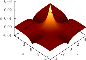
Figure 1: (Color online) The unnormalized wave function $\psi(x,y)$ satisfying eq. (2). The distances are in units $2/(m\alpha)$.

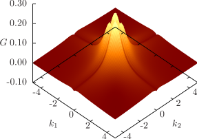
Figure 2: (Color online) The Fourier transform $G(k_{1},k_{2})$ of the ground state position-space wave function $\psi(x,y)$ of eq. (2) computed numerically. The Fourier space coordinates have units $m\alpha/2$.

The result $\varepsilon=-2/3$ translates into the energy eigenvalue $E$ equal $-1/3$ atomic unit of energy (1 a.u. $=m\alpha^{2}$) or $-9.07$ eV. This is in qualitative agreement with the actual value that is about $-0.26$ a.u., just below $-1/4$ a.u. (this fraction is the binding energy of a positronium atom in the non-relativistic approximation).

We note that the eigenvalue that can be obtained for the two-body problem (the positronium or the hydrogen atom) in the one dimensional delta model coincides precisely with the physical value. This is the case because the wave function in the delta model has the same cusp at the origin as the radial wave function in the physical space. Thus the delta model reproduces that radial wave function exactly. For the three-body problem the agreement is only rough.

It would be interesting to determine the one dimensional wave function analytically. We remark that the Schrödinger equation of the three body problem (2) can be rewritten, with a simple change of variables $x,y$, in the form of a one-particle motion in the external potential consisting of two attractive and one repulsive delta function ridges.

In the following section we focus on the opposite limit of very many dimensions. We shall find that an expansion around that limit can be constructed, giving a very accurate determination of the binding energy of $\mathrm{Ps}^{-}$. Interestingly, the $D=1$ method will be again useful: it will provide an important subtraction term that we will use to accelerate the convergence of a perturbative expansion.

III $D\rightarrow\infty$ and Dimensional Perturbation Theory

The first step in taking the $D\rightarrow\infty$ limit is to generalize the Ps^- Schrödinger equation to $D$ dimensions. We are interested in the ground state, which is completely described by the three inter-particle distances $\rho_{ij}=|\vec{r}_{i}-\vec{r}_{j}|$. The Schrödinger equation takes the form

$$H\phi\equiv(T+U+V)\phi=E\phi,$$ (9)

where $E$ is the energy in atomic units $m\alpha^{2}$ (note that it differs by a factor 1/2 from the $\varepsilon$ used in $D=1$ in the previous section) and

$$T = -\frac{1}{2}\sum_{i\neq j}\left(\frac{\partial^{2}}{\partial\rho_{ij}^{2}}+\sum_{k\neq i,j}\frac{\rho_{ij}^{2}+\rho_{ik}^{2}-\rho_{jk}^{2}}{2\rho_{ij}\rho_{ik}}\frac{\partial^{2}}{\partial\rho_{ij}\partial\rho_{ik}}\right),$$

$$U = \frac{(D-1)(D-5)}{8\Upsilon^{2}}\left(\rho_{13}^{2}+\rho_{23}^{2}+\rho_{12}^{2}\right),$$

$$V = \frac{1}{\rho_{12}}-\frac{1}{\rho_{13}}-\frac{1}{\rho_{23}},$$ (10)

and $\phi=\Upsilon^{(D-1)/2}\psi$ is the rescaled wave function with

$$\Upsilon = 2\sqrt{s(s-\rho_{12})(s-\rho_{13})(s-\rho_{23})},$$ (11)

$$s = \frac{1}{2}(\rho_{12}+\rho_{13}+\rho_{23}).$$ (12)

Note that the characteristic $D^{2}$ dimensional dependence is confined to $U$. (The $U$ term in the effective potential is the usual centrifugal contribution from the kinetic energy found by expressing the Laplacian in terms of $\rho_{ij}$.) In order to obtain a finite limit the coordinates and the energy must be rescaled, $\rho_{ij}=D^{2}r_{ij}$ and $E=\epsilon/D^{2}$. This introduces a factor of $1/D^{2}$ in front of the kinetic energy term, eq. (10), so in the limit $D\rightarrow\infty$ it is suppressed. In terms of the rescaled quantities, the Schrödinger equation is written as

$$(\delta^{2}T+\delta^{2}U+V)\phi=\epsilon\phi,$$ (13)

where $\delta=1/D.$

In the limit $\delta\rightarrow 0$, terms containing derivatives vanish in eq. (13). Since the ground state energy is the smallest eigenvalue of the Hamiltonian, we seek to minimize the effective potential

$$V_{\mathrm{eff}}=\delta^{2}U+V$$ (14)

at $\delta=0$, under the constraint that $r_{ij}$ define a triangle. Unfortunately, in $D\to\infty$, the Ps^- system described by the potential in eq. (10) is unbound (even if the positron were very heavy, its charge would have to be larger than 1.228 for a bound state to exists PhysRevA.51.R5 (see also Hogaasen:2010 ; PhysRevA.71.052505 )). The qualitative explanation of this is that even though we have increased the number of spatial dimensions, we have retained the $1/r$ behavior of the Coulomb potential. Thus it is relatively stronger at large distances than in three dimensions and the electron-electron repulsion plays a more important role even if the electrons are on the opposite sides of the positron.

However, the strict $\delta=0$ regime is unphysical. We are interested in the $\delta=1/3$ case, so we are free to modify the potential as long as it reduces to the correct form at $\delta=1/3$. This can be done by reducing the strength of the electron-electron repulsion, as was done for H^- PhysRevA.51.R5 ,

$$V=\frac{\lambda_{0}+3(1-\lambda_{0})\delta}{r_{12}}-\frac{1}{r_{13}}-\frac{1}{r_{23}},$$ (15)

where $\lambda_{0}$ is a free numerical parameter. Note that at $\delta=1/3$, eq. (15) reduces to eq. (10), as required. We have used $\lambda_{0}=0.5$ throughout our computations since this value gave the best results for the H^- system, but other values of $\lambda_{0}$ may result in better convergence of the perturbation series for $\mbox{Ps}^{-}$. The effective potential, eq. (14), is minimized at

$$\bar{r}_{12} = 0.773603828324(1),$$

$$\bar{r}_{13}=\bar{r}_{23} = 0.5866862922582(4),$$ (16)

with the minimum value of $V_{0}=-1.381325607963162(1)$. The errors are estimated by performing the calculation again with higher precision and smaller tolerances. Convergence is ensured by restarting the minimization from a slightly perturbed location. We note that this result corresponds to the energies rescaled by $\delta^{2}$. Thus, to compare with the physical value, we have to divide this result by $3^{2}=9$, obtaining the first estimate of the binding energy $\simeq-0.15$ a.u., to be compared with the known value (see Table 2) of about $-0.26$ a.u.

The static $\delta=0$ limit is the zeroth order in $1/D$ expansion but, without the kinetic energy, it does not allow us to generate further orders in the perturbation expansion. In order to construct such an expansion, we consider the next simplest case, the harmonic approximation to the potential. This will yield a complete set of states that can be used to generate an expansion. The natural expansion parameter for eq. (13) is $\delta^{1/2}$. This follows from the dominant balance argument applied to the Schrödinger equation. One finds that, for $\delta^{1/2}$, the harmonic terms in the expansion of the potential are of the same order as the constant coefficient terms in the kinetic energy expansion.

Details of the procedure used to construct the expansion are described in the Appendix. The summation of the resulting series in powers of $\delta=1/D$ is complicated by the fact that the expansion is divergent at high orders due to a singularity at $\delta=0$ elout:5112 , so we expect the convergence of the naive summation

$$E(\delta)=\delta^{2}\sum_{k=0}^{\infty}E_{k}\delta^{k}$$ (17)

to be slow. In the above expression $E_{0}=V_{0}$ and $E_{k}=\epsilon_{2k-2}$ for $k>0$, where $\epsilon_{k}$ are expansion coefficients of the rescaled energy that appears in eq. (13). There are also poles at $D=1$ that slow down the asymptotic convergence of the expansion at low values of $D$. A better estimate for $E$ can be obtained by subtracting these poles from the expansion. To this end, the residues of the poles must be determined. Following PhysRevA.51.R5 ; elout:5112 we define

$$E(\delta)=\delta^{2}\left[\frac{a_{-2}}{(1-\delta)^{2}}+\frac{a_{-1}}{1-\delta}+\sum_{k=0}^{\infty}E_{k}^{\prime}\delta^{k}\right],$$ (18)

where

$$E_{k}^{\prime}=E_{k}-(k+1)a_{-2}-a_{-1}.$$ (19)

The residue of the second order pole, $a_{-2}$, corresponds to the ground state energy in the $D=1$ limit (more precisely $a_{-2}=4E_{D=1}$). We have computed it employing again the method described in Section II, this time with the rescaled charges of electrons and the positron so as to satisfy eq. (15). We find

$$a_{-2}=-1.102499999999999(1),$$ (20)

which again (see Table 1) resembles a rational number, indicating that there are likely analytical solutions of the $D=1$ model even for an arbitrary charge of the positron (not necessarily equal in magnitude to that of the electron). As in Table 1, the uncertainty in this converged residue is due to finite precision, as was checked by using larger quadrature sizes.

To find the residue of the single pole, $a_{-1}$, we subtract the double pole from both sides of eq. (18) and multiply by $1-\delta$. We get the condition

$$a_{-1}=\lim_{\delta\rightarrow 1}\sum_{k=0}^{\infty}(E_{k}-E_{k-1}-a_{-2})\delta^{k},$$ (21)

where $E_{-1}=0$. In practice we only have a finite number of terms in the sums in equations (18) and (21). Padé approximants have been shown to work well for summing up $1/D$ expansions PhysRevA.46.5428 ; PhysRevA.51.R5 . Using this method to compute the limit in eq. (21) we get for Ps^-,

$$a_{-1}=0.427(2).$$ (22)

This result was obtained with the first 21 terms in the sum in eq. (21). The uncertainty in the computed value was estimated by varying the order of the Padé approximant for $a_{-1}$ as $[N/M]\rightarrow[(N-1)/(M+1)]$ PadeEncyclopedia . If the result has converged, the order of the approximant should not matter (barring the introduction of spurious poles in the denominator of the approximant). We use this method to estimate the error for all quantities computed using Padé approximants. In our calculations we use the full unrounded result for $a_{-1}$ which gives a slightly worse result for the bound state energy than eq. (22). As has been noted in Ref. PhysRevA.46.5428 , this way of determining $a_{-1}$ is not very accurate. An exact value for $a_{-1}$ (in principle obtainable from expansions about $D=1$) would improve the convergence of the $1/D$ expansion. For He we used $a_{-2}=-3.15546$ rosenthal to get $a_{-1}=0.313(1)$ using an identical calculation with 21 energy expansion coefficients. We then evaluated eq. (18) (with the summation truncated again at 21 terms) at $\delta=1/3$. For helium, this yields a ground state energy that agrees with the variational calculation of korobov2002 to five digits, which is consistent with the result of goodson:8481 for this summation method and perturbation expansion cutoff. The same calculation for the positronium ion yields a five digit agreement with the results in frolov2006 ; Frolov2007 ; Puchalski:2007ck . These results are summarized in Table 2.

	Known energy (1 a. u. = $m\alpha^{2}$)	$1/D$ Expansion
He	$-2.9037243770341196$ korobov2002	$-2.90374(1)$
Ps-	$-0.2620050702329801$ Frolov2007	$-0.262005(2)$

Table 2: Results of summation of the $1/D$ expansion using Padé summation with first and second order poles removed. The first $21$ non-zero terms were used in the summation.

Figure 3 shows the improvements to the energy that are obtained by summing more terms. Higher orders yield better accuracy despite the poor behaviour of the $1/D$ expansion coefficients (see Table 3). In fact, the pole subtraction and Padé resummation described above are necessary to get a sensible answer.

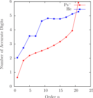
Figure 3: (Color online) Number of accurate digits in the ground state energy, defined as $-\log_{10}[(E-E_{\mbox{\footnotesize exact}})/E_{\mbox{\footnotesize exact}}]$ as a function of the number of terms in the summation of eq. (18).

Aside from computing higher orders in perturbation theory, precision of the result may be improved by using a different summation method. For example, Ref. goodson:8481 found that Padé-Borel summation gives better results for helium than Padé summation.

IV Conclusions

We have investigated the viability of dimensional scaling for making accurate predictions for the positronium ion system. Equal masses and correlation strengths make $\mbox{Ps}{}^{-}$ a good candidate for the dimensional scaling treatment. We considered the $D=1$ limit and found that the Schrödinger equation can be reduced to a one dimensional integral equation. The numerical solution for the energy eigenvalue approaches a simple rational number suggesting the possibility of a completely analytical solution. While this energy is not physically relevant by itself, it can be used to accelerate the convergence of the $1/D$ perturbation series.

We constructed such a perturbative series by expanding the solution of the full Schrödinger equation about the $D\rightarrow\infty$ limit. Each coefficient was computed exactly in the harmonic basis. To obtain an accuracy of five significant figures required expanding up to order $41$ in perturbation theory. While the accuracy of the energy expansion at this order is not yet competitive with variational calculations, the present method provides a valuable alternative approach to few body systems. It can be used to check a variety of matrix elements that have previously been computed only variationally.

In the future, higher orders in the $1/D$ perturbation series can be determined without sacrificing speed if the analytical expansions can be replaced with numerical evaluations of series coefficients through finite differencing. It would also be very valuable to establish how the convergence of this expansion depends on the value of the parameter $\lambda_{0}$ introduced in eq. (15). Finally, the accuracy of the obtained wave function should be determined by evaluating matrix element of various operators and comparing them with the variational approach.

Appendix A Perturbative expansion in $1/D$

In this Appendix we describe how the coefficients of the $1/D$ expansion were determined. Our procedure follows the matrix method of ref. dunn:5987 . In terms of the displacement coordinates $x_{i}$ defined by

$$r_{12} = \bar{r}_{12}+\delta^{1/2}x_{1}$$

$$r_{13} = \bar{r}_{13}+\delta^{1/2}x_{2}$$

$$r_{23} = \bar{r}_{23}+\delta^{1/2}x_{3},$$ (23)

($\bar{r}_{ij}$ are the coordinates of the minimum of the effective potential, eq. (16)), the Schrödinger equation takes the form

$$(\delta T+V_{\mathrm{eff}})\phi=\epsilon\phi.$$ (24)

The Hamiltonian is expanded in powers of $\delta^{1/2}$ such that

$$T = \sum_{i=0}^{\infty}T_{i}\delta^{i/2},$$ (25)

$$V_{\mathrm{eff}} = \sum_{i=0}^{\infty}V_{i}\delta^{i/2}.$$ (26)

Since the expansion is about the minimum of $V_{\mathrm{eff}}$, there is no linear term in its expansion and $V_{1}=0$. Also the kinetic energy $T$ starts contributing only in the second order in $\delta^{1/2}$, so the energy $\epsilon$ has the form

$$\epsilon=V_{0}+\delta\sum_{i=0}^{\infty}\epsilon_{i}\delta^{i/2},$$ (27)

For second order in $\delta^{1/2}$ in eq. (24) we have

$$T_{0} = -{1\over 2}\sum_{i+j+k=2}t_{ijk}\left(\frac{\partial}{\partial x_{1}}\right)^{i}\left(\frac{\partial}{\partial x_{2}}\right)^{j}\left(\frac{\partial}{\partial x_{3}}\right)^{k},$$

$$V_{2} = v_{000}+\sum_{i+j+k=2}v_{ijk}x_{1}^{i}x_{2}^{j}x_{3}^{k},$$ (28)

where $t_{ijk}$ and $v_{ijk}$ are expansion coefficients that are functions of $\bar{r}_{ij}$. This order in perturbation theory corresponds to three coupled harmonic oscillators. To solve the Schrödinger equation they need to be decoupled.This procedure yields normal mode frequencies $\omega_{i}$ and the corresponding normal coordinates $q_{i}$, related to $x_{i}$ by a linear transformation $S$,

$$q_{i}=\sum_{j=1}^{3}(S^{-1})_{ij}x_{j}.$$ (29)

In terms of coordinates $q_{i}$,

$$T_{0} = -\frac{1}{2}\sum_{i=1}^{3}\frac{\partial^{2}}{\partial q_{i}^{2}},$$ (30)

$$V_{2} = v_{000}+\frac{1}{2}\sum_{i=1}^{3}\omega_{i}^{2}q_{i}^{2}.$$ (31)

Defining

$$H_{i}=T_{i}+V_{i+2},$$ (32)

the Hamiltonian can be written as

$$H=\delta T+V_{\mathrm{eff}}=V_{0}+\delta\sum_{i=0}^{\infty}H_{i}\delta^{i/2}.$$ (33)

Next we consider the wave function expansion

$$\phi=\sum_{i=0}^{\infty}\phi_{i}\delta^{i/2}.$$ (34)

Without loss of generality $\phi_{i}$ can be normalized as

$$\langle\phi_{0}|\phi_{j}\rangle=\delta_{0,j}.$$ (35)

Collecting like powers of $\delta^{\frac{1}{2}}$ in eq. (24) yields

$$\sum_{i=0}^{p}(H_{i}-\epsilon_{i})\phi_{p-i}=0.$$ (36)

The $p=0$ order equation is a system of three independent harmonic oscillators with the solution

$$\phi_{0} = h_{\nu_{1}}(q_{1})h_{\nu_{2}}(q_{2})h_{\nu_{3}}(q_{3}),$$ (37)

$$\epsilon_{0} = v_{000}+\sum_{i=1}^{3}\left(\nu_{i}+\frac{1}{2}\right)\omega_{i},$$ (38)

with

$$h_{\nu}(q_{i})=\sqrt[4]{\frac{\omega_{i}}{\pi}}\frac{1}{\sqrt{2^{\nu}\nu!}}H_{\nu}\left(\sqrt{\omega_{i}}q_{i}\right)e^{-\omega_{i}q_{i}^{2}/2},$$ (39)

where $H_{\nu}$ is the $\nu$’th Hermite polynomial. For the ground state, $\nu_{i}=0$.

To compute further orders in the perturbation expansion, $\phi_{j}$ from eq. (34) are projected onto the harmonic oscillator basis

$$\phi_{j}=\sum_{i_{1},i_{2},i_{3}}{{}_{j}}a^{i_{1}i_{2}i_{3}}h_{i_{1}}(q_{1})h_{i_{2}}(q_{2})h_{i_{3}}(q_{3}).$$ (40)

Here ${{}_{j}}a^{i_{1}i_{2}i_{3}}$ are the expansion coefficients. The advantage of using the Hermite function basis is that only a finite basis at every order of perturbation theory is needed, since the perturbations are polynomials in $q_{i}$. Thus the perturbation expansion coefficients can be computed exactly. We note that ${}_{0}a^{i_{1}i_{2}i_{3}}=\delta_{0,i_{1}}\delta_{0,i_{2}}\delta_{0,i_{3}}$. Equation (35) then implies that for any $p>0$

$${{}_{p}}a^{000}=0.$$ (41)

The matrix elements of the operators $H_{j}$ defined in eq. (32) are computed by noting that each $H_{j}$ is a sum of terms of the form

$$q_{1}^{i_{1}}q_{2}^{i_{2}}q_{3}^{i_{3}}\left(\frac{\partial}{\partial q_{1}}\right)^{\alpha_{1}}\left(\frac{\partial}{\partial q_{2}}\right)^{\alpha_{2}}\left(\frac{\partial}{\partial q_{3}}\right)^{\alpha_{3}},$$ (42)

where $\alpha_{1}+\alpha_{2}+\alpha_{3}=2$ for the kinetic terms and $\alpha_{i}=0$ for terms coming from $V_{\mathrm{eff}}$. The matrix elements of $q_{i}$ and $\frac{\partial}{\partial q_{i}}$ are derived from the recurrence relations of the Hermite functions dunn:5987 ,

$$q_{i} = \frac{1}{\sqrt{2\omega_{i}}}\left(\begin{array}[]{ccccc}0&\sqrt{1}&0&0\\ \sqrt{1}&0&\sqrt{2}&0\\ 0&\sqrt{2}&0&\sqrt{3}&\cdots\\ 0&0&\sqrt{3}&0\\ &&\vdots&&\ddots\end{array}\right),$$ (48)

$$\frac{\partial}{\partial q_{i}} = \sqrt{\frac{\omega_{i}}{2}}\left(\begin{array}[]{ccccc}0&\sqrt{1}&0&0\\ -\sqrt{1}&0&\sqrt{2}&0\\ 0&-\sqrt{2}&0&\sqrt{3}&\cdots\\ 0&0&-\sqrt{3}&0\\ &&\vdots&&\ddots\end{array}\right),$$ (54)

so $H_{j}$ is a linear combination of direct products of such matrices. We denote the matrix representation of $H_{j}$ by $\mathbf{H}_{j}$, and by $\mathbf{a}_{j}$ the tensor with elements ${}_{j}a^{i_{1}i_{2}i_{3}}$ in the harmonic basis. Finally we derive the recursion relations for computation of the energy and wave function expansion coefficients. First, we rewrite eq. (36) in the harmonic basis

$$\sum_{i=0}^{p}(\mathbf{H}_{i}-\epsilon_{i})\mathbf{a}_{p-i}=0,$$ (55)

and then contract with $\mathbf{a}_{0}$ and solve for $\epsilon_{p}$, which yields

$$\epsilon_{p}=\mathbf{a}_{0}\sum_{i=1}^{p}\mathbf{H}_{i}\mathbf{a}_{p-i}.$$ (56)

To compute the wave function expansion coefficients we need the pseudo-inverse $\mathbf{K}$ of the operator $\mathbf{H}_{0}-\epsilon_{0}$, defined component-wise as

$$\mathbf{K}_{i_{1}i_{2}i_{3}}^{k_{1}k_{2}k_{3}}=\begin{cases}0&i_{\alpha}=k_{\alpha}=0\mbox{ }\forall\alpha\\ \left(\sum_{j=1}^{3}\omega_{j}i_{j}\right)^{-1}\delta_{i_{1}i_{2}i_{3}}^{k_{1}k_{2}k_{3}}&\mbox{otherwise}\end{cases}.$$ (57)

The operator $\mathbf{K}$ is defined such that $\mathbf{K}(\mathbf{H}_{0}-\epsilon_{0})=1$ everywhere except for the subspace spanned by the harmonic ground state wave function $\phi_{0}$, where the inverse of $\mathbf{H}_{0}-\epsilon_{0}$ would be undefined and it is convenient to choose $\mathbf{K=}0$. Contracting $\mathbf{K}$ with eq. (55) gives

$$\mathbf{a}_{p}=\mathbf{K}\sum_{i=1}^{p}(\epsilon_{i}-\mathbf{H}_{i})\mathbf{a}_{p-i}.$$ (58)

Together equations (56) and (58) allow us to compute the ground state energy and wave function to any order.

We implemented the steps required to compute the $1/D$ expansion to arbitrary order in Mathematica mathematica and in C++. The determination of the Taylor expansion coefficients of the Hamiltonian is done with Mathematica. The computation of the perturbation series (eqs. (56) and (58)) is done in C++, for its speed of operations with large arrays (corresponding to the various tensor contractions in these equations). We have computed $20$ $1/D$ expansion coefficients (which required expanding up to order $41$ in perturbation theory). The result is presented in Table 3. Also in this table are the corresponding coefficients for helium (from an identical calculation), which agree to at least five significant figures with Table I of goodson:8481 (after accounting for a difference in units, which amounts to diving by $Z^{2}=4$) and serve as a check of our calculations. Note that the coefficients in Table 3 become large at high orders. This is due to the essential singularity at $\delta=0$. The nature of this singularity has been investigated in Ref. goodson:8481 .

Due to the large number of algebraic operations required to generate the $1/D$ expansion we need to check for round off error in our coefficients; one way to do this is to repeat the C++ computation at higher precision (there should be no need to redo the Mathematica part, since Mathematica does arbitrary precision computations by default, as long as one does not invoke numerical solvers). We have implemented a version of the C++ code using the arbitrary precision arithmetic package ARPREC Bailey02arprec:an .

$p$	$\epsilon_{p}$ for $\mbox{Ps}{}^{-}$	$\epsilon_{p}$ for He
$0$	$-1.185438078904337(1)$ E0	$-2.423036748379509(1)$ E1
$2$	$-2.78770519314798(1)$ E0	$-3.544873487874171(2)$ E1
$4$	$-7.2695509791874(1)$ E0	$-5.56025516084019(2)$ E1
$6$	$6.7347904088005(2)$ E1	$-2.174685942637(1)$ E1
$8$	$-2.1412953632562(1)$ E3	$-3.30958097736(1)$ E2
$10$	$7.8884951280128(7)$ E4	$5.2508188805(2)$ E2
$12$	$-3.519438146299(1)$ E6	$4.0504015254(2)$ E4
$14$	$1.842029153744(1)$ E8	$-1.7333557830(1)$ E6
$16$	$-1.107117203726(1)$ E10	$5.6857880174(1)$ E7
$18$	$7.51651405108(1)$ E11	$-1.77525788344(2)$ E9
$20$	$-5.69017274005(1)$ E13	$5.528541546(1)$ E10
$22$	$4.75290730575(1)$ E15	$-1.732045588(2)$ E12
$24$	$-4.34262756760(1)$ E17	$5.409411228(4)$ E13
$26$	$4.30867078063(3)$ E19	$-1.638399579(2)$ E15
$28$	$-4.6135902290(1)$ E21	$4.4914966(2)$ E16
$30$	$5.3029755999(1)$ E23	$-8.6523653(2)$ E17
$32$	$-6.512769125044(1)$ E25	$-1.289717(2)$ E19
$34$	$8.5114570184(2)$ E27	$3.152243(3)$ E21
$36$	$-1.17941098599(2)$ E30	$-2.796124(6)$ E23
$38$	$1.7272349225(1)$ E32	$2.031490(1)$ E25
$40$	$-3.253630209(1)$ E34	$-1.705787919969(3)$ E33

Table 3: $1/D$ energy expansion coefficients in eq. (27), in units of $m\alpha^{2}$. Terms with odd $p$ vanish. Letter E indicates powers of 10 multiplying the entries. The uncertainty in each coefficient was estimated using a similar calculation with $20$ digit precision as described in the text.

The relative effect of round off error is shown in Fig. 4. We see that the error introduced by finite precision arithmetic is much smaller than the accuracy of the final ground state energy obtained by resumming the $1/D$ expansion. Higher order calculations will require better precision when the fractional error becomes of the same order as the accuracy required.

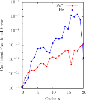
Figure 4: (Color online) Fractional error in the $1/D$ expansion coefficients defined as $|(E_{n}^{(16)}-E_{n}^{(20)})/E_{n}^{(20)}|$ as a function of the order $n$. The coefficients $E_{n}^{(16)}$ were obtained using the standard double precision arithmetic ($\approx 16$ digits of precision), while $E_{n}^{(20)}$ were obtained using the ARPREC arbitrary precision library (with $20$ digits of precision).

References

- (1) A. P. Mills, Phys. Rev. A 24, 3242 (1981).
- (2) J.-M. Richard, Phys. Rev. A 80, 054502 (2009).
- (3) A. Basu, in press in Eur. Phys. J. D, http://dx.doi.org/10.1140/epjd/e2011-20277-x (2011).
- (4) S. Kar and Y. Ho, Comp. Phys. Comm. 182, 119 (2011).
- (5) J. A. Wheeler, Ann. N. Y. Acad. Sci. 48, 219 (1946).
- (6) A. P. Mills, Jr., Phys. Rev. Lett. 46, 717 (1981).
- (7) A. K. Bhatia and R. J. Drachman, Phys. Rev. A 28, 2523 (1983).
- (8) Y. K. Ho, Phys. Rev. A 48, 4780 (1993).
- (9) A. M. Frolov, Phys. Rev. A 60, 2834 (1999).
- (10) A. M. Frolov, Phys. Rev. E 74, 027702 (2006).
- (11) A. M. Frolov, J. Phys. A 40, 6175 (2007).
- (12) G. W. F. Drake and M. Grigorescu, J. Phys. B 38, 3377 (2005).
- (13) M. Puchalski, A. Czarnecki, and S. G. Karshenboim, Phys. Rev. Lett. 99, 203401 (2007).
- (14) A. K. Bhatia and R. J. Drachman, Phys. Rev. A 75, 062510 (2007).
- (15) F. Fleischer et al., Can. J. Phys. 83, 413 (2005).
- (16) A. P. Mills, Jr., Phys. Rev. Lett. 50, 671 (1983).
- (17) F. Fleischer et al., Phys. Rev. Lett. 96, 063401 (2006).
- (18) F. Fleischer, The negative ion of positronium: Decay rate measurements and prospects for future experiments, in S. Karshenboim (ed.), Precision Physics of Simple Atoms and Molecules, Lecture Notes in Physics Vol. 745, pp. 261–281, Springer, Berlin, 2008.
- (19) D. R. Herschbach, J. Avery, and O. Goscinski (eds.), Dimensional Scaling in Chemical Physics (Kluwer Academic Publishers, Dordrecht, 1992).
- (20) M. Dunn et al., J. Chem. Phys. 101, 5987 (1994).
- (21) D. Z. Goodson, M. López-Cabrera, D. R. Herschbach, and J. D. Morgan III, J. Chem. Phys. 97, 8481 (1992).
- (22) D. Z. Goodson and D. R. Herschbach, Phys. Rev. A 46, 5428 (1992).
- (23) D. K. Watson and D. Z. Goodson, Phys. Rev. A 51, R5 (1995).
- (24) E. Witten, Physics Today 33, 38 (1980).
- (25) D. J. Doren and D. R. Herschbach, Phys. Rev. A 34, 2654 (1986).
- (26) J. B. McGuire, J. Math. Phys. 5, 622 (1964).
- (27) E. H. Lieb and W. Liniger, Phys. Rev. 130, 1605 (1963).
- (28) C. N. Yang, Phys. Rev. Lett. 19, 1312 (1967).
- (29) T. W. Craig, D. Kiang, and A. Niégawa, Phys. Rev. A 46, 2271 (1992).
- (30) Y.-Q. Li and Z.-S. Ma, Phys. Rev. B 52, R13071 (1995).
- (31) C. M. Rosenthal, J. Chem. Phys. 55, 2474 (1971).
- (32) D. J. Doren and D. R. Herschbach, J. Chem. Phys. 87, 433 (1987).
- (33) H. Høgaasen, J.-M. Richard, and P. Sorba, Am. J. Phys. 78, 86 (2010).
- (34) T. Li and R. Shakeshaft, Phys. Rev. A 71, 052505 (2005).
- (35) M. O. Elout et al., J. Math. Phys. 39, 5112 (1998).
- (36) G. A. Baker, Jr. and P. Graves-Morris, Padé approximants, 2nd ed. (Cambridge Univ. Press, Cambridge, UK, 1996).
- (37) V. I. Korobov, Phys. Rev. A 66, 024501 (2002).
- (38) S. Wolfram, Mathematica 7 (Wolfram Research Inc., Champaign, Illinois, 2008).
- (39) D. H. Bailey, Y. Hida, X. S. Li, and O. Thompson, ARPREC: An arbitrary precision computation package, http://crd.lbl.gov/ dhbailey/dhbpapers/arprec.pdf, 2002.