A Radiation Transfer Solver for Athena using Short Characteristics

Abstract

We describe the implementation of a module for the Athena magnetohydrodynamics (MHD) code which solves the time-independent, multi-frequency radiative transfer (RT) equation on multidimensional Cartesian simulation domains, including scattering and non-LTE effects. The module is based on well-known and well-tested algorithms developed for modeling stellar atmospheres, including the method of short characteristics to solve the RT equation, accelerated Lambda iteration to handle scattering and non-LTE effects, and parallelization via domain decomposition. The module serves several purposes: it can be used to generate spectra and images, to compute a variable Eddington tensor (VET) for full radiation MHD simulations, and to calculate the heating and cooling source terms in the MHD equations in flows where radiation pressure is small compared with gas pressure. For the latter case, the module is combined with the standard MHD integrators using operator-splitting: we describe this approach in detail, including a new constraint on the time step for stability due to radiation diffusion modes. Implementation of the VET method for radiation pressure dominated flows is described in a companion paper. We present results from a suite of test problems for both the RT solver itself, and for dynamical problems that include radiative heating and cooling. These tests demonstrate that the radiative transfer solution is accurate, and confirm that the operator split method is stable, convergent, and efficient for problems of interest. We demonstrate there is no need to adopt ad-hoc assumptions of questionable accuracy to solve RT problems in concert with MHD: the computational cost for our general-purpose module for simple (e.g. LTE grey) problems can be comparable to or less than a single timestep of Athena’s MHD integrators, and only few times more expensive than that for more general (non-LTE) problems.

1. Introduction

Radiation is of fundamental importance for the thermodynamics of most astrophysical systems. It can be the dominant source of heating and cooling of astrophysical plasmas. Even in those systems where it plays a minor role in energy transport, it is the dominant mechanism through which we perceive and explore the universe. Nevertheless, it has often proven difficult to directly model the effects of radiation accurately in modern multidimensional astrophysical (magneto)hydrodynamic (MHD) codes due to both computational expense and conceptual complexity.

Most approaches to adding radiative transfer to dynamical simulations are based on adopting restrictive assumptions or approximations. For example, often the flow is assumed to be optically thin to radiation everywhere and for all time, or the radiation field is assumed to originate in a small number of point sources, with the diffuse emission from scattered or reradiated photons ignored (such as in Cosmological reionization problems e.g.Abel & Wandelt 2002; Mellema et al. 2006; Rijkhorst et al. 2006; Whalen & Norman 2006; Reynolds et al. 2009; Finlator et al. 2009).

For problems in which the diffuse emission cannot be ignored, the dynamics of the radiation field is often treated by solving the radiation moment equations using ad hoc closure prescriptions to handle the transition from optically thick to optically thin regimes, such as flux-limited diffusion (e.g. Levermore & Pomraning, 1981, hereafter FLD). This includes applications such as accretion flows, star formation, neutrino transport in supernovae, stellar atmospheres and winds, cosmological reionization, and many others. Indeed, there is a large and growing list of astrophysical MHD codes that utilize FLD or a similar prescribed closure relation (including e.g. Turner & Stone, 2001; Bruenn et al., 2006; Hayes et al., 2006; González et al., 2007; Krumholz et al., 2007a; Gittings et al., 2008; Swesty & Myra, 2009; Commerçon et al., 2011; van der Holst et al., 2011; Zhang et al., 2011).

Numerical methods for directly solving radiative transfer (RT) have been implemented (e.g. Stone et al., 1992; van Noort et al., 2002; Hayes & Norman, 2003; Hubeny & Burrows, 2007), but their application to astrophysical problems has been somewhat limited, especially in full 3D. A notable exception is the progress made in simulating the atmospheres of the Sun and other cool stars. In the solar physics community, multidimensional MHD simulations of convection with realistic RT have been performed for decades with increasing sophistication. (see e.g. Nordlund, 1982; Stein & Nordlund, 1998; Vögler et al., 2005; Heinemann et al., 2007; Hayek et al., 2010)

Encouraged by recent work modeling the departure of the radiation field from local thermodynamic equilibrium (LTE) due to the presence of electron scattering in three-dimensional MHD simulations (see e.g. Hayek et al., 2010), we have implemented a general-purpose RT solver in Athena (Stone et al., 2008), based on the methods widely used in the stellar atmospheres community. Athena is a general purpose astrophysical MHD code, which is being actively developed and already includes several modules for handling a variety of physical processes. Effectively, we have combined Athena with a modern stellar atmospheres code. In fact, Athena already has a RT module that computes the effects of ionization radiation from a single point source on the surrounding gas (Krumholz et al., 2007b). However, this module is not well-suited for modeling the radiation from diffuse continuum emission.

The addition of a RT solver to Athena enables three goals: (1) it can be used as a diagnostic tool to compute self-consistently spectra and images from time-dependent MHD simulations for direct comparison to astronomical observations; (2) it allows us to compute a variable Eddington tensor (VET) for the integration of the coupled MHD and radiation moment equations (Sekora & Stone 2010; Jiang et al., submitted to ApJS, hereafter JSD12) for full radiation MHD simulations in regimes where both energy and momentum transport by photons is important; and (3) it allows us to compute the radiation source terms in the energy equations and directly couple them to the MHD integrator to compute the dynamics of flows where radiation pressure can be ignored.

This paper focuses on describing our implementation of methods to solve the RT equation, and the coupling of the solver with the MHD integrator to compute the radiation source term in the energy equation. The computation of the VET and solution of the radiation moment equations is described in JSD12. The plan of this work is as follows: In Section 2 we summarize the equations that are solved. In section 3 we describe the detailed implementation of our solver and the iterative methods used model deviations from LTE and handle certain (e.g. periodic) boundary conditions. In section 4 we describe how we compute the radiation source terms in the energy equation and incorporate them into the MHD integration. In Section 5 we present the results of several test problems not only to assess the accuracy of the RT solver, but also to evaluate the performance of the MHD integrator when the energy source terms are included. We summarize our results in Section 6.

2. MHD Equations with RT

In this work we solve the usual equations of compressible MHD, including the source term in the energy equation to account for heating and cooling due to radiation. These source terms are computed directly from a formal solution of the time-independent RT equation. Thus, the basic equations are continuity

$$\frac{\partial\rho}{\partial t}+\mathbf{\nabla}\cdot\left(\rho\mathbf{v}\right)=0,$$ (1)

momentum conservation

$$\frac{\partial\left(\rho\mathbf{v}\right)}{\partial t}+\mathbf{\nabla}\cdot\left(\rho\mathbf{v}\mathbf{v}+{\sf T}\right)=0,$$ (2)

the induction equation

$$\frac{\partial\mathbf{B}}{\partial t}-\mathbf{\nabla}\times\left(\mathbf{v}\times\mathbf{B}\right)=0,$$ (3)

and energy conservation

$$\frac{\partial E}{\partial t}+\mathbf{\nabla}\cdot\left(E\mathbf{v}+{\sf T}\cdot\mathbf{v}\right)=Q_{\rm rad}.$$ (4)

In the above, $\rho$ is the gas density, $p$, $\mathbf{v}$ is the fluid velocity, and $\mathbf{B}$ is the magnetic field. The total stress tensor $\sf T$ is defined as

$${\sf T}=(p+B^{2}/2){\sf I}-\mathbf{B}^{\rm T}\mathbf{B},$$ (5)

and $E$ is the total (fluid) energy

$$E=\frac{p}{\gamma-1}+\frac{1}{2}\rho v^{2}+\frac{B^{2}}{2},$$ (6)

where $p$ is the gas pressure and $\sf I$ is identity matrix.

The source term on the right hand side of equation (4) is the net gain or loss of energy due to radiative heating and cooling and is given (for a static medium) by

$$Q_{\rm rad}=4\pi\int^{\infty}_{0}\chi^{\rm tot}_{\nu}\left(J_{\nu}-S_{\nu}\right)d\nu.$$ (7)

This is an integral over frequency $\nu$ of the difference between mean intensity $J_{\nu}$ and the total source function $S_{\nu}$, weighted by the total opacity We do not attempt to add the corresponding radiation source term to the momentum equation. This limits us to applications in which radiation pressure is at most a modest fraction of gas pressure. An integrator for the coupled MHD and radiation moment equations based on the one-dimensional algorithms discussed in Sekora & Stone (2010) has been implemented in Athena and extended to multidimensions by JSD12. These more advanced techniques are needed to handle the stiff source terms and modified dynamics in radiation pressure dominated flows.

In order to compute the energy source term due to radiation, the MHD equations must be supplemented by the time-independent equation for RT

$$\hat{n}\cdot\nabla I_{\nu}=\chi^{\rm tot}_{\nu}\left(S_{\nu}-I_{\nu}\right),$$ (8)

where $I_{\nu}$ is the specific intensity for an angle defined by the unit vector $\hat{n}$. In this work, we consider opacities due to scattering $\chi^{\rm sc}_{\nu}$ and true absorption $\chi^{\rm abs}_{\nu}$, with $\chi^{\rm tot}_{\nu}=\chi^{\rm abs}_{\nu}+\chi^{\rm sc}_{\nu}$. It is convenient to define the photon destruction probability $\epsilon_{\nu}=\chi^{\rm abs}_{\nu}/\chi^{\rm tot}_{\nu}$. The source function is then given by

$$S_{\nu}=\epsilon_{\nu}B_{\nu}+(1-\epsilon_{\nu})J_{\nu},$$ (9)

where $B_{\nu}$ is thermal source function. The mean intensity $J_{\nu}$ is the “zeroth” moment, or average, of $I_{\nu}$ over solid angle

$$J_{\nu}=\frac{1}{4\pi}\int I_{\nu}(\hat{n})d\Omega.$$ (10)

When absorption dominates $\epsilon_{\nu}\rightarrow 1$ and $S_{\nu}\rightarrow B_{\nu}$, but when scattering dominates $\epsilon_{\nu}\rightarrow 0$ and $S_{\nu}\rightarrow J_{\nu}$. Note that this expression assumes that scattering is isotropic. Although this is not strictly true for many scattering processes (e.g. electron scattering), it will generally be a good approximation for problems of interest.

In addition to $J_{\nu}$ we will also use ${\bf H}_{\nu}$ and ${\sf K}_{\nu}$, the first and second moments, respectively. Their components are given by

$$H^{i}_{\nu} = \frac{1}{4\pi}\int I_{\nu}(\hat{n})\mu_{i}d\Omega,$$ (11)

$$K^{ij}_{\nu} = \frac{1}{4\pi}\int I_{\nu}(\hat{n})\mu_{i}\mu_{j}d\Omega,$$ (12)

where $d\Omega$ is the differential of solid angle, and $\mu_{i}\equiv\hat{n}\cdot\hat{x}_{i}$. These moments are related to the radiation energy density $E_{\rm rad}$, radiation flux $\mathbf{F}_{\rm rad}$, and radiation pressure ${\sf P}_{\rm rad}$ via the standard definitions

$$E_{\rm rad} = \frac{4\pi}{c}\int^{\infty}_{0}J_{\nu}d\nu,$$ (13)

$$\mathbf{F}_{\rm rad} = 4\pi\int^{\infty}_{0}\mathbf{H}_{\nu}d\nu,$$ (14)

$${\sf P}_{\rm rad} = \frac{4\pi}{c}\int^{\infty}_{0}{\sf K}_{\nu}d\nu.$$ (15)

Integration of equation (8) over solid angle yields

$$-\mathbf{\nabla}\cdot\mathbf{F}_{\rm rad}=4\pi\int^{\infty}_{0}\chi^{\rm tot}_{\nu}\left(J_{\nu}-S_{\nu}\right)d\nu.$$ (16)

and provides an alternative (differential) form for the radiation source term in equation (4). The differential form tends to perform better in regions where optical depths across a gridzone are large, while the integral form is preferable in regions of low optical depth. Hence, we will use both expressions, as discussed in section 4.

We have not been forced to make distinctions between the Eulerian and comoving frame for radiation variables as we have dropped all velocity dependent terms in equations (7), (8), and (16). We neglect these terms because they are negligible for the tests considered in this paper. However, we anticipate solving problems where the velocity dependent terms may be important and can implement terms that are first order in $v/c$ in our RT solver, where necessary. For consistency with the VET solver (JSD12), we will adopt the mix frame approach where $I_{\nu}$, its moments, $\nu$, and $\hat{n}$ are Eulerian frame variables, while opacities and emissivities are defined in the comoving frame. Derivations of the mixed frame equations can be found in Mihalas & Klein (1982), Mihalas & Mihalas (1984), Lowrie et al. (1999), and Hubeny & Burrows (2007).

Since we neglect the time derivative of $I_{\nu}$ and terms that are first order in $v/c$ in equation (8), our method is only formally reliable in the static diffusion and free streaming-limits. Specifically, the timescale for fluid flow $t_{\rm f}\sim L/v$ across a characteristic length scale $L$ in the simulation domain must be longer than the time it takes for radiation to diffuse $t_{\rm dif}\sim L^{2}\chi^{\rm tot}/c$ or free-stream $t_{\rm fs}\sim L/c$ across the domain (see e.g. Mihalas & Mihalas, 1984)). This is sufficient for the test problems considered here and should be adequate for many of the problems of primary interest to us. When necessary, we can retain terms first order in $v/c$ in equations (7) and (8) and the code will be formally accurate in the dynamic diffusion limit ($t_{\rm f}\lesssim t_{\rm dif}$) as well.

Throughout this work $B_{\nu}$ is assumed to correspond to the Planck function and is a function only of $\nu$ and gas temperature $T$. We assume an ideal equation of state with $p=\rho RT$ and gas thermal energy density $E_{\rm gas}=p/(\gamma-1)$. Here $R$ is the gas constant and $\gamma$ is the adiabatic index. The adiabatic sound speed is $a=\sqrt{\gamma p/\rho}$.

The methods for solving the MHD equations without the radiation source term are described in detail in previous publications (Gardiner & Stone, 2008; Stone et al., 2008; Stone & Gardiner, 2009) and are unchanged by the solution of radiation transfer. The computation of RT is described in Section 3 and the interface of the RT solver and MHD integrator is described in Section 4. The sequence for a single timestep can summarized as follows:

1) Using the hydrodynamic variables (typically $T$ and $\rho$) from the previous timestep as inputs, we compute $\chi^{\rm tot}_{\nu}$, $\epsilon_{\nu}$, and $B_{\nu}$, or each frequency in each grid zone.

2) We solve Equation (8) using the methods described in Section 3, yielding $S_{\nu}$ and $J_{\nu}$ everywhere in the domain.

3) Using $S_{\nu}$ and $J_{\nu}$ (or $H_{\nu}$), we compute the radiation source term $Q_{\rm rad}$ and update equation (4) as described in Section 4.

4) We advance the MHD variables using the standard Athena integrators.

3. Solution of Radiation Transfer

An extensive literature on the solution of RT for astrophysical problems in multidimensions exists and there are numerous monographs and review articles on the topic (e.g. Mihalas & Mihalas, 1984; Castor, 2004; Carlsson, 2008). With this literature to draw from, we have largely adopted a strategy of implementing existing, well-developed algorithms. Since there are many different methods with different strengths and weaknesses, the major challenge is finding a method which best suits our particular needs. Our most salient constraints include:

1) The method needs to be amenable to domain decomposition since this is the primary algorithm for parallelizing the solution of the MHD equations in Athena.

2) The method must be able to handle the explicit dependence of the source term on $J_{\nu}$ in equation (9) for problems in which scattering is important (i.e. we must be able solve non-LTE problems).

3) The method needs to be able to handle (shearing) periodic boundary conditions.

4) The method must be robust and capable of handling discontinuities in temperature and density which arise when shocks are present in the flow.

5) Ideally, the method should be efficient enough that for simple problems (e.g. LTE with grey or mean opacities), neither the memory constraints nor the total computational time is dominated by the solution of RT.

With these considerations in mind, we have implemented a short-characteristics based solver (Mihalas et al., 1978; Olson & Kunasz, 1987; Kunasz & Auer, 1988). In this method the specific intensity is discretized on a set of rays at each cell center in the simulation domain. Equation (8) is integrated along each ray using initial intensities interpolated from neighboring grid zones. Since only neighboring grid zones are used for this integration, the total computational cost (per iteration) scales linearly with the number of gridzones in the domain. This is also simple to parallelize with domain decomposition as only information from cells on the faces of the neighboring sub-domains need to be passed.

This is in contrast to a long characteristics method (e.g. Feautrier, 1964), which would integrate the RT equation along each ray through all gridzones intersected by the ray until the edges of the simulation domain are reached. Such a method is generally more computationally expensive since computation of the specific intensity in each gridzone typically requires integrating equation (8) through $\sim N^{1/3}$ gridzones (where $N$ is the total number of gridzone in the domain). It is also more cumbersome to use with domain decomposition (see, however, Heinemann et al., 2006) since it may require the passing of larger blocks of data, including information from non-neighboring subdomains.

Although short characteristic methods are computationally more expedient, they suffer from greater numerical diffusion due to the interpolation that is required to compute the intensity in neighboring gridzones (Kunasz & Auer, 1988). For problems where a few gridzones (or point sources) dominate the total emissivity, a short characteristics solver may require very high angular resolution to accurately resolve the radiation field far from the dominant source. If the angular resolution is too low, anomalous structure (e.g. spokes) in the heating and cooling rates will emanate from the dominant sources (see e.g. Finlator et al., 2009). (In this case the numerical diffusion introduced by interpolation can be beneficial.) Instead, the emission from point sources is better handled by suitably designed long characteristics methods (Abel & Wandelt 2002; Krumholz et al. 2007b, although see also Rijkhorst et al. 2006). For the applications of interest in this work (e.g. accretion flows), the diffuse radiation field dominates. Moreover, even when point sources are present, the diffuse radiation field due to scattering or re-emission (e.g. HII regions) cannot generally be ignored, and therefore we anticipate such problems may be accommodated in the future by a hybrid scheme which uses short characteristics for the diffuse emission, and long characteristics for bright point sources.

Non-LTE problems are handled via iteration. For each time step the formal solution of the whole domain is repeated, updating $J_{\nu}$ and $S_{\nu}$ during each iteration, until some formal convergence criterion is met. As discussed below, we implement an accelerated (or approximate) lambda iteration (hereafter ALI) algorithm based on the Gauss-Seidel method of Trujillo Bueno & Fabiani Bendicho (1995) (hereafter TF95). The TF95 method is efficient for solving non-LTE problems because it significantly increases the convergence rate without significantly increasing the computational cost (or memory footprint) per iteration.

Iteration is also used in LTE problems to handle boundary conditions at the interface of subdomains and for physical periodic boundary conditions at domain edges. On each iteration the incoming intensity from the neighboring subdomain is fixed from the previous iteration (or timestep for the first iteration). The outgoing intensity, which corresponds to the incoming intensity in the neighboring subdomain, is then updated and the formal solution is iterated to convergence. For LTE problems, this is not the most efficient method for handling the subdomain boundaries (see e.g. Heinemann et al., 2006). For the moment, we are primarily interested in non-LTE problems where iteration is required regardless. We generally find fairly rapid convergence (requiring only a few iterations) for most of our LTE test problems when iterations is used, so this is not a significant limitation.

In many respects our short-characteristics RT solver is similar to those of van Noort et al. (2002) and Hayek et al. (2010) in that both implement ALI to handle deviations from LTE and both utilize domain decomposition for parallelization. Hayek et al. (2010) used their code to solve the RT equation including scattering, in MHD simulations of stellar atmospheres on three-dimensional Cartesian grids. Hence, the effectiveness of several key aspects of our module have already been demonstrated in a sophisticated MHD code and applied to realistic astrophysical applications.

3.1. Frequency Discretization

The scheme we have implemented allows for the computation of frequency dependent, grey, or monochromatic RT. Radiation variables (moments and specific intensities) and radiative properties of the fluid such as the opacities, thermal source function, and photon destruction parameter are tabulated on a grid of $n_{\rm f}\geq 1$ discrete frequencies or frequency groups. For flexibility, the functional form of opacities and emissivities can be specified via user-defined functions. In general, the computational cost and memory footprint of problems scale linearly with $n_{\rm f}$.

These frequency bins can simply be discrete frequencies when RT is used to generate diagnostic outputs such as images and spectra. Group mean opacities and emissivities (e.g. Mihalas & Mihalas, 1984; Skartlien, 2000) and corresponding quadrature weights must be specified when the RT solver is used to compute the radiation source terms or VET. In the simplest case, $n_{f}=1$ and an appropriate frequency integrated mean opacity is specified.

Unless otherwise noted, we will drop subscripts denoting the frequency dependence of radiation variables and only describe the monochromatic problem hereafter. For the problems under present consideration, there is no explicit coupling of the specific intensity at different frequencies so the frequency dependent calculation is a trivial generalization of the monochromatic problem.

3.2. Angular Discretization

We discretize the specific intensity on both angular and spatial grids. For one-dimensional problems, the discretization is chosen so that polar angles correspond to the abscissas for Gaussian quadrature. In multidimensions, discretization of the angles proceeds according to the algorithm described in Appendix B of Bruls et al. (1999), which is based on the principles of type A quadrature described in Carlson (1963).

This method attempts to distribute the rays as evenly as possible over the unit sphere, subject to the constraint that each octant of the unit sphere is discretized identically. Hence the angle discretization is invariant for 90^∘ rotations about the coordinate axes. This is desirable because Athena is designed to be a general purpose code, and there is often no preferred direction with which to align the angular grid (as in some atmosphere calculations). Without this constraint, the result would generally depend on the orientation of boundary and initial conditions relative to the coordinate axes.

The user specifies the number of polar angles $n_{\mu}$, and the code generates an array of $n_{\rm a}$ rays covering the unit sphere. In one dimension, this corresponds to $n_{\rm a}=n_{\mu}$ rays because of axisymmetry. For multidimensional domains $n_{\rm a}=n_{\mu}(n_{\mu}+2)$ rays. However, in two-dimension only half of these are unique due to the implied invariance of physical quantities in the third dimension and $n_{\rm a}=n_{\mu}(n_{\mu}+2)/2$.

Setting $n_{\mu}=2$ in a one-dimensional calculation is analogous to invoking the two-stream approximation, in which the radiation field of each hemisphere is approximated by transfer along a single ray. This assumption is commonly used to derive analytic solutions, and allows the ratio of $H/J$ to vary but keeps the ratio of $K/J$ fixed at 1/3, consistent with the Eddington approximation. In two (three) dimensional calculations, choosing $n_{\mu}=2$ approximates each quadrant (octant) with a single ray and also yields $K_{ij}=1/3\delta_{ij}J$. The algorithm is well-defined and unique only for $n_{\mu}\leq 12$ (Bruls et al., 1999), corresponding to $n_{\rm a}=168$ (84 in two dimensions). This should not be prohibitive for the problems of interest.

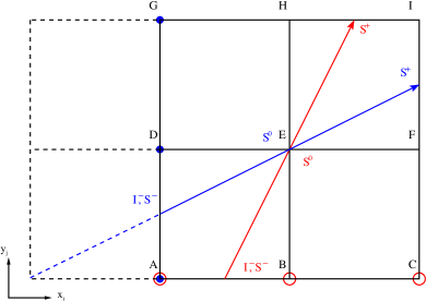
Figure 1.— Schematic of the RT solution for an individual gridzone whose cell center correspond to vertex E in a two-dimensional radiation grid. In this case $S^{0}$, and $\chi^{0}$ are known at E, and $I^{0}$ is to be computed. $I^{0}$ is computed along a each ray using equation (20). Since quantities $I^{-}$, $S^{\pm}$, and $\chi^{\pm}$ do not correspond to vertices of the grid, they must be computed via interpolation from neighboring grid zones. The red ray intersects rows between vertices A and B (upwind) or H and I (downwind). Hence the values of $S$, $\chi$ and $I$ at these vertices are used to interpolate $S^{\pm}$, $\chi^{\pm}$, and $I^{-}$. Vertices C and G are also used with quadratic interpolation. A similar case holds for the blue ray, but with interpolation performed on columns A-D-G and C-F-I. The open and closed circles denote vertices which are used for the interpolation of $I^{-}$. The dashed curve is an extension of the blue ray which intersects A-B-C row.

For each ray $\hat{n}_{k}$, we compute a vector of direction cosines $(\mu_{0k},\mu_{1k},\mu_{2k})$ with $\mu_{ik}=\hat{n}_{k}\cdot\hat{x}_{i}$ and quadrature weights $w_{k}$. Then equations (10)-(12) become

$$J = \sum_{k=0}^{n_{a}-1}w_{k}I_{k}$$ (17)

$$H_{i} = \sum_{k=0}^{n_{a}-1}w_{k}I_{k}\mu_{ik}$$ (18)

$$K_{ij} = \sum_{k=0}^{n_{a}-1}w_{k}I_{k}\mu_{ik}\mu_{jk},$$ (19)

where $I_{k}\equiv I(\hat{n}_{k})$.

3.3. Implementation of the Short-Characteristics Algorithm

The short characteristic method (Mihalas et al., 1978; Olson & Kunasz, 1987; Kunasz & Auer, 1988) has been discussed previously by several authors. The basic computation step for a single gridzone in both LTE and non-LTE problems is illustrated in Figure 1 for the two-dimensional case. Fluid radiative properties and radiation variables (e.g. $\chi^{\rm tot}$, $B$, $\epsilon$, $I_{k}$, $J$, $S$) are defined on a radiation grid. The vertices of this grid correspond to the cell centers of the MHD domain so that fluid radiative properties are computed directly from the cell centered MHD fluid variables. Generalizing to three dimensional domains is straight-forward.

At each vertex, the specific intensity $I^{0}_{k}$ at $\mathbf{x}^{0}$ is computed along each ray $\hat{n}_{k}$ from $\mathbf{x}^{-}_{k}$ to $\mathbf{x}^{+}_{k}$. For second-order interpolation the intensity is given by

$$I^{0}_{k} = I^{-}_{k}e^{(-\Delta\tau^{-}_{k})}+\Psi^{-}_{k}S^{-}_{k}+\Psi^{0}_{k}S^{0}+\Psi^{+}_{k}S^{+}_{k},$$ (20)

where $\Psi^{-}_{k}$, $\Psi^{0}_{k}$, and $\Psi^{+}_{k}$ denote interpolation coefficients which depend on the opacities $\chi^{-}_{k}$, $\chi^{0}$, and $\chi^{+}_{k}$ through the optical depth intervals $\Delta\tau^{-}_{k}$ and $\Delta\tau^{+}_{k}$.

The form of the interpolation coefficients $\Psi^{-}_{k}$, $\Psi^{0}_{k}$, and $\Psi^{+}_{k}$ depends on the interpolation method used. The standard expressions for second order interpolation are listed in equations (7a)-(9c) of Kunasz & Auer (1988). One drawback of these expression is that they are subject to overshoot where gradients in $S^{\pm}_{k}$ and $\chi^{\pm}_{k}$ are steep. Fortunately, these cases can be handled with Bézier-type interpolation as described in Auer (2003) and Hayek et al. (2010). With Bézier-type interpolation schemes, one can utilize a control point $S^{\rm c}_{k}=S^{0}-0.5\Delta\tau^{-}_{k}(\partial S/\partial\tau)^{0}_{k}$ to determine if overshoots are present in the standard second-order expressions. If $S^{\rm c}_{k}<{\rm min}(S^{-}_{k},S^{0})$ or $S^{\rm c}_{k}>{\rm max}(S^{-}_{k},S^{0})$ overshoots are present and alternative expressions are utilized. Suitable choices follow from setting $S^{\rm c}_{k}=S^{-}_{k}$ or $S^{\rm c}_{k}=S^{0}$. Hayek et al. (2010) provide the corresponding expressions for $\Psi^{\pm}_{k}$ and $\Psi^{0}_{k}$ in their Appendix A. Similar methods are also used to compute intervals $\Delta\tau^{\pm}_{k}$ (see e.g. equation A.3 of Hayek et al. 2010).

For one-dimensional problems, $\mathbf{x}^{-}_{k}$ and $\mathbf{x}^{+}_{k}$ correspond to neighboring grid vertices $x_{i-1}$ and $x_{i+1}$. Hence, $I^{-}_{k}=I_{i-1,k}$, which was just computed in the neighboring zone while $S^{\pm}_{k}$, and $\chi^{\pm}_{k}$ can be computed directly from hydrodynamics variables at $x_{i\pm 1}$. In multidimensional problems, $\mathbf{x}^{-}_{k}$ and $\mathbf{x}^{+}_{k}$ no longer correspond to vertices of the radiation grid and variables $I^{-}_{k}$, $S^{\pm}_{k}$, and $\chi^{\pm}_{k}$ must be interpolated. We implement and test both first-order (linear) and monotonic second order (quadratic) interpolation schemes (Auer & Paletou, 1994). Both methods prevent overshoots and enforce positivity of the interpolants. The choice is particularly relevant for $I_{k}$, as second-order methods generally produce much less diffusion of the radiation beam. A drawback of second order interpolation is that it places additional constraints on the order in which one sweeps through gridzones and the stencil used for the evaluation of $I_{k}$.

Consider the two rays depicted in Figure 1. We compute interpolants $S^{\pm}_{k}$ and $\chi^{\pm}_{k}$ using known quantities at vertices of the radiation grid. If row A-B-C or column A-D-G correspond to ghost (boundary) zones, $I_{k}^{-}$ can be computed from the (prescribed) boundary intensities. If they are not ghost zones, interpolation can only be performed on zones in which $I_{k}$ has already been computed. If we first sweep along rows of fixed $y_{j}$ (as in Figure 2), $I_{k}$ has only been computed at vertices A, B, C, and D. This means that $I_{k}$ is known for all vertices used in the linear interpolation of $I^{-}_{k}$ as well as for quadratic interpolation (and any higher order interpolation) of rays which intersect row A-B-C.

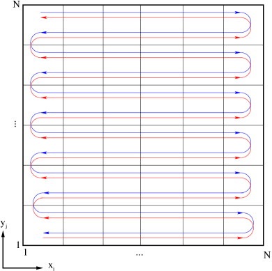
Figure 2.— Progression of the sweep through a two-dimensional grid (domain or subdomain) when linear interpolation is used. The forward sweep (red curve) first progresses parallel to $\hat{y}$, computing RT only for upward pointing rays ($\hat{n}\cdot\hat{y}>0$). For each row (fixed $y_{j}$), one first sweeps parallel to $\hat{x}$, computing RT along rays with $\hat{n}\cdot\hat{x}>0$ until reaching the grid edge $x_{N}$, then reverses direction and computes along rays with $\hat{n}\cdot\hat{x}<0$ until reaching the grid edge $x_{0}$. This continues until one reaches gridzone $(x_{0},y_{N})$. The backward sweep (blue curves) inverts the forward sweep, computing RT only for downward pointing rays ($\hat{n}\cdot\hat{y}<0$). In the Gauss-Seidel method, updated values of $S_{i,j}$ are incorporated into the backward sweep, beginning with $S_{N,N}$. The three-dimensional case is a straightforward generalization.

We refer to rays that intersect the column A-D-G, such as the blue one in Figure 1, as “shallow” rays. Shallow rays are a potential problem for quadratic (and higher order) interpolation, since $I_{k}$ at G has not been computed. When quadratic or higher order interpolation is desired, such rays can be handled in a number of ways. One possibility is to switch the order of the sweep for shallow rays so that it first proceeds in the y direction along columns of fixed $x_{i}$. In this case $I_{k}$ for shallow rays will be known at vertices A, B, D, and G. The main drawback (discussed further in Section 3.4 below) is that one is unable to implement a Gauss-Seidel iteration for non-LTE problems.

One can also construct alternatives by extending the stencil beyond vertices A-I. For example, one can extend shallow rays until they intersect row A-B-C as shown by the dashed curve in Figure 1. A drawback of this solution is that it requires modest additional effort for computing $\Psi^{-}_{k}$, although this can be alleviated by computing only on the first iteration and reusing it for subsequent iterations (e.g. Hayek et al., 2010). Alternatively quadratic interpolation could be preformed using A, D, and the vertex directly below A (Kunasz & Auer, 1988).

These two solutions share common drawbacks. For parallelization with domain decomposition, only one ghost zone is needed per grid zone on a subdomain face, when only vertices A-I are used. Extension of shallow rays beyond this stencil requires the passing of additional data and associated bookkeeping. More philosophically, we feel it is desirable to treat all rays as consistently as possible. In either of these schemes, RT along some rays will be computed using only neighboring grid zones, while other rays will not. Our preference is to treat all rays on the same footing.

For this reason, we have decided to switch the order of the sweep for shallow rays. Athena is implemented so that each sub-grid of the domains has regular spacing and therefore gridzones with fixed aspect ratio. This means that the distinction between rays that are shallow and those that are not is equivalent for each grid zone. However, our definition of a shallow ray depends upon the direction of the sweep. The blue ray in Figure 1 is shallow because we first traverse the grid along rows of fixed $y_{j}$, only moving to $y_{j+1}$ when intensity has been computed for all gridzones in the row $y_{j}$, as depicted in Figure 2.

If we reverse the sweep so that we first traverse columns of fixed $x_{i}$, the blue ray will no longer be shallow, as the intensity at G will be computed before it is needed for the computation of the intensity at E. In this case the red ray is now a shallow ray as the intensity at C will not have been computed before it is needed to compute the intensity at E. Hence, by varying the sweep direction, we can handle all rays and accommodate a quadratic interpolation scheme which computes all intensities in a gridzone $(x_{i},y_{j})$ only using intensities from neighboring gridzones $(x_{i\pm 1},y_{j\pm 1})$.

3.4. Iterative Methods for Non-LTE Problems

We now describe how we handle non-LTE problems iteratively. Following common convention we denote the angle averaged formal solution of the RT equation (hereafter, simply the formal solution) in operator notation as

$$J=\Lambda S.$$ (21)

Here, $\Lambda$ is a linear operator representing the (discretized) formal solution, and $J$ and $S$ are vectors spanning each gridzone in the simulation domain. Using equation (9) to eliminate $J$, one obtains an equation for $S$ in terms of $B$

$$S=(1-\epsilon)\Lambda[S]+\epsilon B.$$ (22)

Since $\Lambda$ is a linear operator we can solve for $S$

$$S=[1-(1-\epsilon)\Lambda]^{-1}[\epsilon B].$$ (23)

If one can invert $\Lambda$ a formal solution of the non-LTE problem follows from solving (23) and obtaining $J$ from (21). However, for three-dimensional problems $\Lambda$ is a very large matrix and not sparsely populated when systems are far from LTE so its direct inversion is impractical. Therefore, equation (22) is usually solved via iteration.

A simple iterative scheme for solving equation (22) begins with an initial guess for the source function $S^{N}$, which is then used to compute an improved estimate $S^{n+1}=(1-\epsilon)\Lambda[S^{n}]+\epsilon B$. However, this method (often referred to as Lambda Iteration) has very poor convergence properties. For practical problems, ALI methods (Cannon, 1973) are commonly used. Rybicki & Hummer (1991), Hubeny (2003) and TF95 provide useful reviews of ALI methods and we refer the reader to these works for a more in-depth discussion. Here we just summarize the basic concepts involved.

In ALI methods one solves equation (23) directly, but using an approximate form $\Lambda^{*}$ which is easier to invert then the full $\Lambda$ operator. Since only the approximate $\Lambda^{*}$ is used, iteration is still necessary. Numerous choices for $\Lambda^{*}$ have been proposed, but it has been argued that simply taking the diagonal elements of the full $\Lambda$ matrix represents a near-optimal choice (Olson et al., 1986). Olson & Kunasz (1987) provide expressions for diagonal elements of $\Lambda$ when short characteristics are used. In each grid zone the change in the source functions $\Delta S_{i}=S^{n+1}_{i}-S^{n}_{i}$ can be written as

$$\Delta S_{i}=\frac{(1-\epsilon_{i})J^{n}_{i}+\epsilon_{i}B_{i}-S^{n}_{i}}{1-(1-\epsilon_{i})\Lambda_{ii}},$$ (24)

where the subscript $i$ enumerates all gridzones in the domain.

As TF95 discuss, when $J^{n}$ is exclusively used in equation (24), the ALI scheme is equivalent to the Jacobi iterative method for solving linear systems. TF95 show that one can construct a Gauss-Seidel algorithm by incorporating the new values of $J^{n+1}_{i^{\prime}<i}$ in equation (24) as these become available. Here $i^{\prime}<i$ refers to gridzones where $J$ has already been updated. The complexity of devising a Gauss-Seidel algorithm for RT comes from the fact that the computation of specific intensity $I_{i,k}$ for some subset of the rays $\hat{n}_{k}$ need to be computed using $S^{n}_{i^{\prime}<i}$ rather than $S^{n+1}_{i^{\prime}<i}$ (i.e. old rather than new values of the source function). Therefore the contribution from these particular rays to $J^{n+1}_{i^{\prime}<i}$ must be corrected as the updated values $S^{n+1}_{i^{\prime}<i}$ become available.

TF95 give a detailed description of how to implement such an algorithm on a one-dimensional domain. The algorithm requires storing a modest amount of data in each gridzone, but very little additional computation. The convergence rate is improved by a factor of two, so problems requiring several iterations gain nearly a factor of two decrease in computational effort for only a minor increase in code complexity.

When linear interpolation is used, the generalization of their one-dimensional method to two and three-dimensional domains is straight-forward. The two-dimensional sweep proceeds as depicted in Figure 2. The vertices in the radiation grid correspond to cell centers $(x_{i},y_{j})$. The sweep generally proceeds with $i$ as the more rapidly varying index. Consider a domain with $N_{x}=N_{y}=N$ for simplicity. In each gridzone $(x_{i},y_{j})$, we first compute the intensity $I_{k}$ for all upward directed rays $(\hat{n}_{k}\cdot\hat{y}>0)$ in the forward sweep and then for all downward directed rays $(\hat{n}_{k}\cdot\hat{y}<0)$ on the reverse sweep.

On the reverse sweep, the upper right gridzone $(x_{N},y_{N})$ is the first in which the computation of all new intensities $I^{n+1}_{k}$ is completed. At this point $J^{n+1}_{N,N}$ is completely specified and we compute $S^{n+1}_{N,N}$. From here on, all subsequent RT computations use $S^{n+1}_{N,N}$ rather than $S^{n}_{N,N}$. However, this alone is not sufficient to make it a Gauss-Seidel scheme, because the contributions to $J^{n+1}_{N-1,N}$, $J^{n+1}_{N,N-1}$, and $J^{n+1}_{N-1,N-1}$ from upward directed rays on the forward sweep used $S^{n}_{N,N}$. These must also be updated using $\Delta S_{N,N}=S^{n+1}_{N,N}-S^{n}_{N,N}$ and weights which were saved on the forward sweep. We also update the outgoing intensities $I^{n+1}_{k}$ (since they were also computed using $S^{n}_{N,N}$) as they correspond to the incoming intensities in neighboring gridzones. Since the corresponding weights have already been computed as part of the forward sweep, the additional computational cost is very modest.

Following the discussion in Section 3.3, we note that feasibility of performing a Gauss-Seidel iteration with quadratic interpolation is dependent on the way shallow rays are handled. Reorienting the sweep for shallow rays so that $j$ is more rapidly varying index, but keeping $i$ as the rapidly varying index for remaining rays does not allow for an efficient Gauss-Seidel scheme because some of the necessary $J^{n+1}$ (and therefore $S^{n+1}$) are not available when the backward sweep begins. In the light of this issue, we have implemented Gauss-Seidel routines only with linear interpolation. For problems where quadratic interpolation is preferable, we default to the Jacobi method (i.e. standard ALI).

We continue the iteration until some convergence criterion is met. Consistent with previous work, we stop iterating when the maximum relative change in the source function over the whole domain is less than some prescribed threshold $\delta_{c}$

$$\max\left(\frac{|\Delta S_{i}|}{S_{i}}\right)\leq\delta_{c}.$$ (25)

For LTE problems that use iteration to handle boundary conditions, $S$ does not change from one iteration to the next and we replace $S_{i}$ with $J_{i}$ in equation (25).

The choice of $\delta_{c}$ is clearly an important input to the method, but there is no firmly established criterion and the optimal choice depends on a number of considerations that may be problem dependent. Since the computational cost of the method generally scales linearly with the number of iterations performed and a lower threshold leads to more iterations, there is a tradeoff between accuracy and computational expediency. With the exception of the uniform temperature non-LTE atmosphere, the tests presented in section 5 were performed using $\delta_{c}=10^{-5}$. Increasing $\delta_{c}$ to $10^{-4}$ had a negligible impact on the linear wave tests.

Our expectations based on the tests we have performed so far are that for the problems of primary interest to us (e.g. shearing box simulations of accretion disks) $\delta_{c}\sim 10^{-5}-10^{-3}$ will be sufficient, consistent with studies using similar methods (e.g. Hayek et al., 2010). However, we emphasize that the appropriate choice will be problem dependent and must be assessed on a case-by-case basis. We view the choice of $\delta_{c}$ in roughly the same terms as we view the choice of grid resolution. One can adopt a threshold based on previous results and experience, but ultimately one needs to compute the problem using a range of $\delta_{c}$ and choose a sufficiently small value such that the results are insensitive to the choice.

3.5. Boundary Conditions and Parallelization

Boundary conditions and domain decomposition in Athena are both implemented for MHD via the use of ghost zones, and we implement RT boundary conditions in an analogous way. The solver computes RT in gridzones on a boundary (domain or subdomain) in the same way as an interior gridzone, but using the intensities and source functions from the ghost zones to compute the relevant integration weights and interpolants. The intensities and source functions in the ghost zones are determined according to prescribed boundary conditions.

In general, boundary conditions for the MHD integrator will not translate directly to boundary conditions for the RT solver. Different problems with the same MHD boundary conditions may require different boundaries for the radiation field. Hence separate boundary conditions must be prescribed when using the RT solver. For the code test problems presented in section 5, we have implemented two types of boundary conditions specifying either fixed incident intensity or periodic intensities on the boundaries. Other boundary conditions can be specified via user defined functions.

Athena runs on parallel machines using domain decomposition implemented through MPI calls. The MHD integrator passes all conserved variables and passive scalars from faces of neighboring subdomains to ghost zones. The MHD integrator requires either four or five ghost zones for each gridzone on the subdomain face. The RT solver operates analogously, passing intensities and source functions, but only requires one ghost zone for each gridzone on a subdomain face.

The main differences between the RT solver and the MHD integrator are the frequency and quantity of data that must be passed. For each frequency bin in every ghost zone $I$ must be passed for all $n_{a}$ rays with quadratic interpolation or, alternatively, $n_{a}/2$ incoming rays with linear interpolation. For non-LTE problems $S$ and $\mathbf{H}$ must also be passed. Hence for quadratic interpolation, the code passes a total of $n_{f}(n_{a}+1+n_{\rm dim})$ floating point variables per face gridzone per iteration, where $n_{\rm dim}$ is the number of dimensions in the domain. In contrast, the MHD integrator typically passes $\sim 50$ floating point variables per face gridzone per timestep. For problems where $n_{a}$ and $n_{f}$ are small and few iterations are required (e.g. an LTE grey problem), the volume of RT data is therefore comparable to and may even be less than the amount of data passed by the MHD integrator.

We note that the use of iteration to handle subdomain boundary conditions may lead to some dependence on the number of subdomains that are used. We have considered the sensitivity of our results to this issue by performing most of the tests described in section 5 both with and without domain decomposition. In practice, the converged mean intensities do not differ (relative to the non decomposed domain) by more than $\sim\delta_{c}J$. The sensitivity is highest for problems where the optical depth across an individual subdomain is of order unity or smaller, Problems with optically thick subdomains generally lead to smaller discrepancies. Since we already choose our convergence criterion to be at a level that minimizes the impact on our results, this sensitivity to the domain decomposition should not lead to significant errors.

4. Interface of the Radiative Transfer Solver to the MHD Integrator

There are two regimes in which the effect of radiation on the MHD is important. The first is when the radiation field is a significant contribution to both the energy and momentum fluxes in the flow. In this regime, the radiation source terms in the MHD equations can be very stiff, and the equations contain wave modes which propagate at close to the speed of light. Both of these properties require significant modification to the underlying MHD integrators in order to enable accurate and stable integration. In JSD12 we describe a method for this regime based on an extension of the modified Godunov method of SS10 to multidimensions, with a VET (defined as ${\sf f}={\sf P_{\rm rad}}/E_{\rm rad}$) computed from a formal solution of the RT equation using the module described in this paper. At each time step, the RT solver computes the radiation field as described in Section 3, evaluating ${\sf K}$ and $J$ via equations (17) and (19). We the compute the VET using ${{\sf f}=\sf K}/J$ as described in section 3.4 of JSD12.

The second regime is when the radiation pressure can be ignored, and the effect of radiation is only through the heating and cooling source terms in the energy equations. In principle, the modified Godunov method adopted in JSD12 would be an attractive approach for handling the stiff energy source term that can arise in this regime as well. However, the modified Godunov method requires that one compute the gradient of radiation source terms on the plane of primitive variables. This in turn requires analytic expression for the radiation sources in terms of the fluid variables. Hence, it is generally not a viable method for problems where the radiation properties are complicated functions of frequency and fluid variables, as may be the case with bound-free and bound-bound atomic opacities or Compton scattering.

These limitations motivate us to implement an alternative method to directly compute the radiation source term in the fluid energy equation (4) and couple it to the standard MHD integrators. When operating in this mode, we perform the formal solution at the beginning of each timestep. We first compute fluid radiation properties in each gridzone $\mathbf{x}_{i}$ of the domain. This includes the variables $\chi^{\rm tot}_{i}$, $B_{i}$, and $\epsilon_{i}$, which are computed via user-defined functions of the conserved MHD variables and passive scalars from the previous timesteps. We use these, along with $J_{i}$ from the previous time-step, to initialize $S_{i}$. Once the formal solution is completed, we account for the source function on the right hand side of equation (4) via an operator split update of $E$. We first compute the radiative source function in each zone and then update the total energy

$$\Delta E_{i}=\delta t(Q_{\rm rad})_{i}.$$ (26)

The standard MHD integration algorithm then proceeds using this “new” value for $E_{i}$.

We compute $Q_{\rm rad}$ in one of two ways, depending on the characteristic optical depth. We either use the integral form

$$Q^{\rm int}_{i}=4\pi\chi^{\rm tot}_{i}(J_{i}-S_{i})=4\pi\chi^{\rm abs}_{i}(J_{i}-B_{i}),$$ (27)

or the differential form

$$Q^{\rm dif}_{i}=-4\pi\mathbf{\nabla}\cdot\mathbf{H}_{i},$$ (28)

Previous work (Bruls et al., 1999, and references therein) has demonstrated that the integral form is inaccurate when the optical depth per gridzone is large. In this case $J_{i}-B_{i}\ll B_{i}$ while $\chi^{\rm abs}_{i}$ is large so round-off errors can be greatly amplified. The integral form, however, is more accurate when $\chi^{\rm abs}_{i}\Delta\mathbf{x}_{i}\lesssim 1$ (Bruls et al., 1999).

Therefore, we have designed our RT solver to compute either form of $Q_{\rm rad}$, depending on the regime of the computation. In most applications of interest, there is a transition from optically thick to optically thin regions, so we must specify a criterion for switching between the differential and integral forms in the same domain. For the test problems considered here, we find a simple switch

$$(Q_{\rm rad})_{i}=\left\{\begin{array}[]{ll}Q^{\rm int}_{i}&{\rm if}\;\chi^{\rm tot}_{i}\Delta x_{i}\leq 1\\ Q^{\rm dif}_{i}&{\rm otherwise}\end{array}\right.$$

to be sufficient. This has the advantage that it is a purely local criterion. Using a method which more smoothly interpolates between the two regimes (see e.g. Hayek et al., 2010) did not improve performance in a measurable way, but may be preferable for more sophisticated applications.

Due to the explicit update, we must take care in choosing a time step. In the absence of radiation the MHD integrator chooses a time step $\delta t_{\rm C}$ based on the CFL constraint. In principle, this time step can be much larger than the radiative cooling time, which could lead to obvious errors, such as the energy density becoming negative. As we elaborate upon in section 5.4, one can derive a generalized CFL condition for a radiating fluid based on the need to resolve the damping time for a non-equilibrium radiation diffusion mode. This time scale $\delta t_{\rm rd}$ is generally most restrictive when the optical depth per gridzone $\chi^{\rm tot}\Delta x\sim 1$, in which case

$$\delta t_{\rm rd}\approx\frac{E_{\rm gas}}{E_{\rm rad}}\frac{a}{c}\delta t_{\rm C},$$ (29)

assuming the adiabatic sound speed $a$ (rather than the Alfvén speed) sets the CFL condition. This generalized CFL constraint can be quite stringent, requiring short time steps and increasing computational costs if either $a\ll c$ or $E_{\rm rad}\gtrsim E_{\rm gas}$. Hence, many problems will require the use of the VET method described in JSD12, which uses timesteps determined by the standard (non-radiative) CFL constraint. In practice, we are almost always limited to problems with $E_{\rm gas}<E_{\rm rad}$, so we do not attempt to include the radiation momentum source term in equation (2) as it is generally small for problems that are computationally feasible with operator splitting.

The algorithm described above will, in general, only be first order convergent. Note that we could construct a second-order scheme when using Athena’s VL+CT integrator (Stone & Gardiner, 2009), by performing the operator split update before the corrector step in the predictor-corrector scheme. However, some of the advantages of the second order convergence will be lost due to the increased diffusivity of the VL+CT relative to the CTU+CT scheme (Gardiner & Stone, 2008). Hence, we have not yet pursued the possibility although it may prove to be a useful avenue for future work.

5. Tests

Our test problems fall into roughly two categories: stand-alone tests of the RT solver on fixed domains and tests of the coupled MHD integrator and RT solver in fully time dependent calculations. The former are particularly useful for evaluating the RT solvers performance on multidimensional and non-LTE problems. For the latter, we focus primarily on simpler LTE problems, so we can compare the simulations result directly to precise analytic or semi-analytic solutions.

Further tests of the RT solver as part of the VET method are presented in JSD12.

Figure 3.— Convergence of the ALI methods on a highly non-LTE uniform atmosphere with $\epsilon=10^{-6}$. The curves show the maximum relative difference between the numerically computed $S$ and the analytic solutions implied by equation (30) for the Jacobi (solid) and Gauss-Seidel (dotted) methods. We compute the numerical solutions using a one-dimensional domain with 9 gridzones per decade in optical depth.

5.1. Uniform Temperature Non-LTE Atmosphere

We begin by solving the monochromatic RT problem in a uniform temperature, one-dimensional scattering dominated atmosphere. This test is particularly useful for evaluating the RT solver’s performance on a non-LTE systems and evaluating the convergence properties of Jacobi and Gauss-Seidel iterative schemes. We adopt the two-stream approximation for the RT solver so we can compare directly with analytic solutions based on the Eddington approximation. Since we assume a uniform opacity $\kappa$ and temperature $T$, the analytic solution is only a function of optical depth $d\tau=\chi dz$, the thermal source function $B$ and photon destruction probability $\epsilon$. With these assumptions the mean intensity $J$ is given by

$$J=B\left(1-\frac{e^{-\sqrt{3\epsilon}\tau}}{1+\sqrt{\epsilon}}\right).$$ (30)

We assume that $\chi\propto\rho$ and $\rho$ increases exponentially (but keep $\epsilon$ constant) with distance from the upper boundary, which has no incoming intensity. This provides an exponential variation in $\tau$ which is well-suited for resolving the transition from LTE to non-LTE within the atmosphere.

Figure 3 shows the convergence of the true error of the numerically derived solutions. This is evaluated as the maximum relative difference $|\Delta S|/S$, with $\Delta S$ the difference of the numerically derived $S$ from the analytic solution. We first consider a one-dimensional domain with $\epsilon=10^{-6}$, as this gives a highly non-LTE atmosphere and facilitates direct comparison with Figure 3 in TF95. We initialize the radiation field to be in LTE everywhere ($J=B$). We consider two different iterative schemes: Jacobi and Gauss-Seidel. As expected, the convergence rate of the Gauss-Seidel methods is nearly a factor of two better than Jacobi. We assume nine gridzones per decade in $\tau$ to match TF95 and our convergence rates agree reasonably well with those shown their Figure 3.

Figure 4.— Comparison of numerical (solid) and analytic (dashed) solutions of the source function monochromatic, uniform non-LTE atmospheres as a function of optical depth. Each set of curves corresponds to a different photon destruction parameter, running from $\epsilon=10^{-2}$ to $10^{-10}$ from top to bottom. We compute the numerical solutions simulations using cubic three-dimensional domains with $64^{3}$ gridzones, distributed over 64 MPI subdomains. The optical depth variation is aligned with the $z$-axis of the simulation domain and the solution is uniform in the horizontal directions.

We have also implemented the successive over-relaxation (SOR) method of TF95, and find rapid convergence, consistent with that shown in Figure 3 of TF95. We have tested SOR on both one-dimensional and two-dimensional domains and find that it is an effective method as long as all boundary intensities are fixed during iteration. However, if the intensities on one of the boundaries vary from one iteration step to the next, the method is generally not stable. For example, instability occurred when we used periodic boundary conditions or when we employed subdomain decomposition. Since most of our primary science goals involve problems that require the use of periodic boundary conditions or domain decomposition, we do not consider SOR a generally viable method for our work. Nevertheless, it may be an effective method for a modest sized problem that can be run serially with fixed boundary intensities.

We next consider the same test problem, but use a cubic three-dimensional domain with $n_{\mu}=2$. We align the variation of density with the $z$ axis of the domain and use periodic boundaries in the horizontal directions. Figure 4 shows a comparison of the numerical and analytical solutions for various choices of $\epsilon$. The agreement between the numeric and analytic solutions is quite good overall, but tends to be poorest at low optical depths. For fixed resolution, the discrepancies with the analytic solution tends to increase as $\epsilon$ decreases and the domain deviates more strongly from LTE. The accuracy of the numerical solution improves with increasing resolution, but the number of iterations needed for convergence increases roughly linearly with resolution. The number of iterations required for convergence also increases as $\epsilon$ decreases. Hence, greater deviations from LTE require a greater number of iterations for convergence, as one would expect.

Figure 5.— Comparison of Athena (diamonds) and Feautrier (solid) emission spectra from the upper boundary of a one dimensional atmosphere. Both calculations assume isotropic electron scattering and free-free (Bremsstrahlung) absorption and emission for a completely ionized H plasma. The intensities are computed using the same angular grid corresponding to abscissas of a 16 point Gauss-Legendre quadrature of the interval (1,1). The plotted intensities (from top to bottom) correspond to $\cos i=$0.10, 0.28, 0.46, 0.62, 0.76, and 0.99. The atmospheres have constant temperature ($10^{6}$ K) and density which varies exponentially with distance, rising from $10^{-6}$ g/$\rm cm^{2}$ at the upper (surface) boundary to $10^{-4}$ g/$\rm cm^{2}$ and lower boundary. For comparison, we plot the corresponding blackbody at $10^{6}$ K as a dashed curve.

Although some RT problems do require explicit frequency coupling (e.g. Compton scattering, partial redistribution), many problems can be treated in the approximation that frequencies are not explicitly coupled. Multifrequency problems are then just a series of single frequency calculations and, hence, a straightforward generalization of the monochromatic problem. Figure 5 shows the intensity spectrum from a multifrequency calculation done with Athena for a uniform temperature atmosphere. We again assume $\rho$ varies exponentially with distance, rising from $10^{-6}$ g/$\rm cm^{2}$ at the upper boundary to $10^{-4}$ g/$\rm cm^{2}$ and lower boundary. The results plotted here are for $N_{x}=256$.

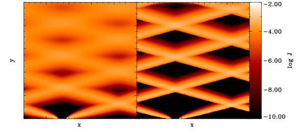
Figure 6.— Mean intensity $J$ due to incident beams propagating through a rarefied, two-dimensional domain. The source function and opacity are zero everywhere and the horizontal boundaries are periodic. The boundary condition at the top and bottom of the domain are zero incident intensity except for two gridzones at the base of the domain. In each of these gridzones $I$ is non-zero for a single ray. The two rays make the same angle with the y-axis, but are oppositely directed in x, with $\hat{n}\cdot\hat{y}=0.174$ and $\hat{n}\cdot\hat{x}=\pm 0.628$. The left and right panels show results from computations with linear interpolation and monotonic quadratic interpolation,respectively.

Incoming intensity at the upper boundary is assumed to be zero and $I_{\nu}=B_{\nu}$ at the lower boundary. We include isotropic electron scattering opacity and free-free (Bremsstrahlung) emission and absorption. The electron scattering is modeled as isotropic and the cross-section is the Thomson cross-section. For simplicity free-free processes are computed assuming a Gaunt factor of unity. The plasma is assumed to be completely ionized Hydrogen. Hence, $\epsilon_{\nu}$, $B_{\nu}$, and $\chi_{\nu}$ are all functions of frequency. However, for an individual frequency the calculations are very similar to those described above. The only difference is that $\epsilon_{\nu}$ is now a function of depth as well, due to the different dependence of scattering and absorption opacity on $\rho$.

Figure 5 also shows the results of a Feautrier calculation for the same atmosphere using the same angular grid. The two calculations generally agree quite well, although there is a tendency for the Athena solver to give slightly higher intensities for frequencies where the spectrum deviates from blackbody. The discrepancy between the results is a function of spatial resolution with agreement between the two codes improves as the $N_{x}$ is increased in the Athena calculation. Calculations on two and three dimensional domains (but with density varying only in one dimension) yield similar results.

5.2. Beam Tests in Two Dimensions

We now consider the propagation of crossing beams of radiation, incident on the boundary of a rarefied ($B=0$, $\chi=0$), periodic domain. This test is particularly useful for evaluating the amount of diffusion associated with the interpolation schemes for the specific intensity. It is also useful testing the performance of periodic and subdomain boundary conditions.

The results for a two-dimensional domain with periodic boundary condition in the horizontal direction are shown in Figure 6. The figure compares a computation with linear interpolation to one with quadratic monotonic interpolation. Our implementation of these methods is described in Section 3.3. It is clear from Figure 6 that linear interpolation leads to substantially greater diffusion of the radiation beam.

Depending upon the application, the additional diffusion in the linear interpolation scheme can be either advantageous or problematic. On one hand, a less diffusive scheme allows one to model important effects, such as shadowing by optically thick material, with greater fidelity. Indeed, the ability to more accurately capture such effects is an important motivation for using RT instead of more ad hoc closure prescriptions, such as FLD.

However, computational expedience limits the angular resolution we can achieve. When only a modest number of rays are used with a less diffusive scheme, fan-shaped “spokes” can appear in the mean intensities and Eddington factors, if the emission in a small number of grid zones significantly exceed that of surrounding zones. Indeed, our short characteristics based method is not well suited to problems with bright point sources for this reason, but even in applications with distributed emission regions, there can be relatively confined regions with larger than averaged emission (e.g. due to magnetic dissipation). In such cases, a greater degree of diffusion in the intensity can mitigate unphysical effects which would otherwise arise due to the limited angular resolution.

A related test of an RT routine is its ability to cast a shadow when an optically thick obstruction is present in the domain. We present such a calculation in Section 5.5 of JSD12, where the ablation of an optically thick cloud is studied. In this case the RT solver was used to compute the radiation field using linear interpolation for the intensity field of neighboring zones. Figure 14 of JSD12 demonstrates that our RT solver can produce sharply defined umbra and penumbra under such conditions. FLD and other approximate moment methods generally fail this test (see e.g. Hayes & Norman, 2003).

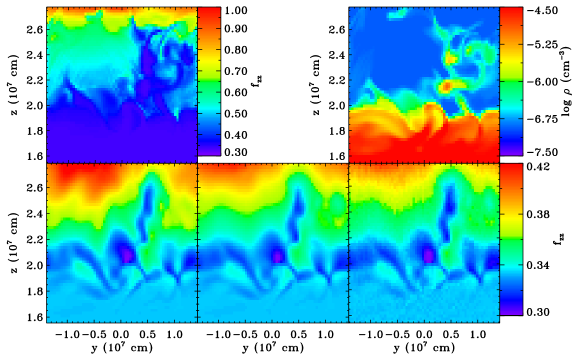
Figure 7.— Comparison of Eddington factors computed using our RT scheme with MC and FLD computations in a representative two-dimensional slice near the top of a three-dimensional domain. We plot the $f_{zz}$ component of the Eddington tensor for computations with our Athena solver using either 24 (bottom, left) or 168 (bottom, center) angle bins, and for the MC (bottom, right) and FLD methods (top, left). We also plot $\rho$ in the same slice for comparison (top, right). Note the larger range for the color bar in the panel showing the Eddington factor for the FLD computation.

5.3. Comparison with Monte Carlo and FLD Methods

We now focus on comparing the performance of our short characteristics solver (referenced throughout this section as the SC method) with two alternative methods: FLD and Monte Carlo (MC). Our motivation is two-fold: in part, we want to evaluate the performance on a fully three dimensional domain, but impose as few restrictive assumptions (e.g. the Eddington approximation) on the radiation field as possible. Since there is a paucity of such truly three dimensional problems with analytic solutions, comparison with alternative RT solution methods is the best alternative. In addition, FLD and MC methods are, in principle, some of the most computationally efficient alternatives to short characteristics solvers, so direct comparison may allow us to assess the relative merits of different methods.

For this comparison we use a three dimensional snapshot from a stratified shearing box simulation, corresponding to a gas pressure dominated patch of an accretion disk (Hirose et al., 2006). This simulation was computed with the Zeus MHD code, using the FLD solver developed by Turner & Stone (2001) and subsequently modified by Hirose et al. (2006). They solved the radiation moment equations using a flux limiter of the type described in Levermore & Pomraning (1981). Further details about the particular snapshot used here can be found in Blaes et al. (2006). From the $E_{\rm rad}$ dump, we compute $F_{\rm rad}$ and the Eddington factor $\sf f$, using finite differences and flux limiters consistent with those employed in the numerical simulation.

We solve the RT equation on this snapshot using both our SC solver and the MC code described in Davis et al. (2009). For both calculations, we assume isotropic electron scattering and monochromatic RT (i.e. a single frequency bin) with mean opacities equal to those used in the Zeus simulation ($\chi^{\rm abs}=3.7\times 10^{53}\rho^{11/2}E_{\rm gas}^{7/2}$ and $\chi^{\rm sc}=0.33\rho$, both in cgs units). We assume no incoming intensity at the surface boundaries and periodicity in the horizontal directions. The latter assumption is inconsistent with the use of shearing periodic boundaries in the radial direction in the numerical simulation, but this does not contribute significantly to the discrepancy between the SC and FLD methods

We compare the radiation moments (${\sf P}_{\rm rad}$, $\sf f$, $\mathbf{H}_{\rm rad}$, and $E_{\rm rad}$) output by the SC/MC solvers with those determined by the FLD method. Independent of the variable used for comparison, we find reasonable agreement between the SC and MC solvers, but discrepancies with the FLD approximation. For brevity we will focus on a single scalar quantity, $f_{zz}$, since it characterizes the variation of angular distribution of the radiation field across methods.

Figure 7 shows a comparison of $f_{zz}$ among the various methods for a representative two-dimensional slice near the top boundary of the simulation domain. In the top row, the left and middle panels show results from the SC solver, using 24 and 168 angles, respectively. The top right panel shows the MC results and the bottom left panel shows the Eddington values computed with the FLD approximation. The bottom right panel shows $\rho$ for the same two-dimensional slice.

We first compare the SC and MC calculations which provide similar results. The consistency of the solution computed by these two very different numerical methods strongly suggests that they are providing accurate results. As can be seen for $f_{zz}$ in Figure 7 the agreement between the radiation moments improves as the angular resolution in the SC solver is increased (i.e. between the top left and top right panels). However, even with higher angular resolution there are some modest discrepancies in the $f_{zz}$ near the surface. This in part due to the statistical noise in the MC calculation, for which S/N generally decreases as $z$ increases. This MC calculation was run with $\sim 12$ billion photon packets with a total computation time that exceeded the SC solver by a factor of $\sim 100$.

Since the improvement in S/N only increases as roughly $\sqrt{N}$, where $N$ is the number of photon packets, further improving S/N involves a substantial increase in the computational time. Even for this rather large number of photon packets, substantial noise remains in the radiation field. Such a high level of statistical noise could lead to numerous problems when coupled to the MHD integrator. Hence, schemes which use MC methods to solve RT will generally require a large number of packets. Our results suggest that standard MC methods need to be much more efficient or parallelized with effective load balancing between the MHD integrator and the MC RT solver to be competitive with SC methods when the simulation domain is far from LTE. Alternatively, it may be possible to significantly improve on this performance by implementing some sort of hybrid MC scheme to handle optically thick regions more efficiently (e.g. Densmore et al., 2007) since a significant fraction of the time in our MC computation is spent solving RT in regions that are very optically thick to scattering (so $f_{zz}\sim 1/3$) but still optically thin to absorption.

There are several discrepancies between the SC/MC and FLD calculations. The most obvious is that with FLD, $f_{zz}$ approaches unity by construction in the optically thin limit. Obtaining $f_{\rm zz}=1$, requires the radiation field to be concentrated in a pencil beam of negligible solid angle around the $z$ axis, and is only achieved on the $z$ axis at very large distances from a finite source. Therefore, it is not appropriate for the upper boundary of a patch of an accretion disk where the radiation field is still rather broadly distributed over solid angle. Indeed, $f_{zz}\sim 0.42$ is consistent with estimates for a scattering dominated semi-infinite atmosphere (Chandrasekhar, 1960). In principle, one could tailor the flux-limiter to approach an alternative, problem dependent value, although one can imagine applications where the appropriate limit will be difficult to estimate a priori.

Furthermore, the FLD results yield $f_{zz}>0.332$ everywhere, but in both the MC and SC calculations $f_{zz}\lesssim 0.3$ is frequently obtained in localized regions, consistent with a more horizontally directed radiation field. It is also clear that the FLD Eddington factors correlate with $\rho$ to a much higher degree that in the SC or MC calculations. Although some correlation is present in the MC and SC calculations as well, it is more prevalent in the optically thick regions and becomes much weaker in the optically thin regions where the radiation field should be more diffuse and more sensitive non-local variations in $T$ and $\rho$.

Further discrepancies between the VET and FLD approaches are discussed in JSD12. The level at which these differences affect the overall dynamics and thermodynamics remains unclear and ultimately requires comparison with full numerical simulations using the SC/VET methods. We note that the horizontally averaged flux in the SC and FLD methods differs by $\lesssim 5\%$ at the top of the domain. Hence the global thermodynamic properties of the simulations may not be greatly modified even though local properties of the radiation field differ. Since simulations of accretion disk dynamics in the shearing box approximation is one of our primary applications, we expect to be able to make direct comparison with FLD-based results (e.g. Hirose et al., 2006) in the near future.

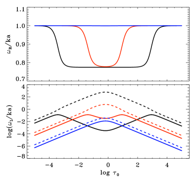
Figure 8.— Real (top) and imaginary (bottom) parts of frequencies of radiatively modified acoustic modes versus optical depth per wavelength $\tau_{0}$. We plot three sets of curves and symbols corresponding to different Boltzmann numbers Bo = 0.01 (black), 1 (red), 10, and 100 (blue). The curves correspond to radiation modified acoustic modes (solid) and a non-equilibrium radiation diffusion mode (dashed). We normalize $\omega_{R}$ and $\omega_{I}$ by the product of the wave number $k$ and the adiabatic sound speed $a$. The real part of $\omega$ is zero for the radiative diffusion mode.

5.4. Radiating Linear Waves

We now turn to tests of the RT solver when coupled to the MHD integrator. We first compute the radiative damping rate of linear (acoustic) waves (Stein & Spiegel, 1967). The closely related problem of the spatial damping of driven harmonic disturbances is covered in Mihalas & Mihalas (1984). We briefly review the derivation of the dispersion relation for such wave and refer the reader to these references for further discussion. We consider an ideal gas with a static, uniform background state in LTE, with a grey absorption opacity $\chi$ and frequency integrated thermal source function $B=\sigma_{\rm B}T^{4}/\pi$. Adopting the notation of Mihalas & Mihalas (1984), we define background and perturbed quantities with subscripts “0” and “1” respectively. The background states has $\mathbf{v}=0$ with $\chi_{0}$ and $I_{0}=J_{0}=B_{0}$ constant everywhere.

With these assumptions and some algebra the linearly perturbed versions of equations (1)-(4) reduce to

$$\frac{\partial T_{1}}{\partial t}-\left(\gamma-1\right)\frac{T_{0}}{\rho_{0}}\frac{\partial\rho_{1}}{\partial t}-\frac{4\pi(\gamma-1)\chi_{0}}{R\rho_{0}}\left(J_{1}-B_{1}\right)=0,$$ (31)

and

$$\left(\frac{\partial^{2}}{\partial t^{2}}-a^{2}_{\rm I}\nabla^{2}\right)\rho_{1}-R\rho_{0}\nabla^{2}T_{1}=0,$$ (32)

where we $a_{\rm I}=a/\sqrt{\gamma}$ is the isothermal sound speed. Similarly, equation (8) becomes

$$\hat{n}\cdot\nabla I_{1}=\chi_{0}\left(B_{1}-I_{1}\right).$$ (33)

Figure 9.— Real (top) and imaginary (bottom) parts of frequencies of radiatively damped linear waves versus optical depth per wavelength $\tau_{0}$. The curves are analytic solutions to eq. (38) and the symbols are estimates derived from simulations. We plot four sets of curves and symbols corresponding to different Boltzmann numbers Bo = 0.1 (dot-dashed, squares), 1 (dashed, triangles), 10 (dotted, crosses), and 100 (solid, diamonds). We normalize $\omega_{R}$ by the product of the wave number $k$ and the adiabatic sound speed $a$.

To linear order we can assume

$$B_{1}=\left(\frac{\partial B}{\partial T}\right)_{0}T_{1}=4B_{0}\frac{T_{1}}{T_{0}},$$ (34)

and solve equation (33) directly to evaluate $J_{1}$ in equation (31). We have

$$I_{1}=\frac{4B_{0}}{T_{0}}\int^{\infty}_{0}T_{1}(\mathbf{x}_{0}-\hat{n}s)e^{-\chi_{0}s}ds,$$ (35)

where is $ds$ is a displacement parallel to $\mathbf{k}$. We consider plane wave solutions of the form $T_{1}\propto e^{i(\omega t-\mathbf{k}\cdot\mathbf{x})}$. Defining $\mu=\mathbf{k}\cdot\hat{n}$ and integrating over solid angle, we obtain (Mihalas & Mihalas, 1984)

$$J_{1}=\frac{4B_{0}T_{1}}{T_{0}}\int^{1}_{0}d\mu\int^{\infty}_{0}dy\cos{(k\mu y/\chi_{0})}\;e^{-y}.$$ (36)

The integral evaluates to

$$J_{1}=\frac{4B_{0}T_{1}}{T_{0}}\frac{\chi_{0}}{k}\tan^{-1}\left(\frac{k}{\chi_{0}}\right).$$ (37)

We can now solve for the dispersion relation using equations (31), (32), and (37)

$$\omega^{3}-i\omega^{2}\nu_{0}\Xi_{0}-\gamma a^{2}_{\rm I}k^{2}+ia^{2}_{\rm I}k^{2}\nu_{0}\Xi_{0}=0,$$ (38)

in agreement with equation (16) of Stein & Spiegel (1967). We have defined

$$\Xi=1-\frac{\chi}{k}\cot^{-1}\left(\frac{\chi}{k}\right),$$ (39)

and

$$\nu=\frac{16\pi\chi B}{E_{\rm gas}},$$ (40)

and the “0” subscript denotes that quantities are evaluated using the background values. To order unity $\nu_{0}$ is the reciprocal of the radiative relaxation time in the background flow.

Figure 10.— Convergence of the norm of L1 error as a function of resolution for linear wave in a one-dimensional domain. The top panel shows the error norm for waves in the adiabatic regime corresponding to Bo=100, $\tau_{0}=0.01$ (crosses); Bo=100, $\tau_{0}=100$ (squares); and Bo=0.1, $\tau_{0}=10^{4}$ (diamonds). The Bottom panels shows the error norm for waves in the isothermal regime corresponding to Bo=0.01, $\tau_{0}=0.01$ (crosses) and Bo=1, $\tau_{0}=1$ (diamonds). The dashed curves show the expected trends for first-order ($N^{-1}$) and second order ($N^{-2}$) convergence.

Figure 8 shows the solutions to equation (38) for various $\tau_{0}\equiv\chi_{0}/k$ (approximately the optical depth per wavelength) and Boltzmann number

$${\rm Bo}=\frac{\rho_{0}c_{p}T_{0}a}{\sigma_{\rm B}T_{0}^{4}}=\frac{16\gamma a\chi_{0}}{\nu_{0}}.$$ (41)

Here $c_{p}$ is the specific heat at constant pressure, so Bo is the ratio of the enthalpy flux (evaluated for $v=a$) to radiative flux. There are two types of modes: radiatively damped acoustic waves (solid and dashed curves) with phase velocity $v_{\rm ph}=\omega_{R}/k$ varying between $a_{I}$ and $a=\sqrt{\gamma}a_{\rm I}$ and a purely damped ($\omega_{R}=0$) non-equilibrium radiation diffusion mode (dotted curve).

The dimensionless ratio $\nu_{0}\Xi_{0}/(ka_{\rm I})$ determines the importance of radiation. When this ratio is small equation (38) reduces to the standard adiabatic dispersion relation with sound speed $a$ and the damping rate is approximately $\nu_{0}(\gamma-1)/(2\gamma)$. For $\nu_{0}\Xi_{0}/(ka_{\rm I})\gtrsim 1$ the phase speed $\omega/k$ decreases, approaching the $a_{\rm I}$ when $k\sim\chi_{0}$ and $\nu_{0}\gg a_{\rm I}k$, and the damping rate is again small compared to $ka$.

For acoustic waves, the damping rate $\omega_{I}\lesssim ak$ for all Bo and $\tau_{0}$. However, this is not true for radiation diffusion mode. For $\tau_{0}\sim 1$, $t^{-1}_{\rm rd}=\omega_{I}\sim\nu_{0}\Xi_{0}$ and transitions to $t^{-1}_{\rm rd}\sim\nu_{0}\Xi_{0}/\gamma$ for $\tau_{0}\gg 1$ or $\tau_{0}\ll 1$. Near $\tau_{0}\sim 1$, $\Xi_{0}\sim 1$, so the maximum decay rate has $t^{-1}_{\rm rd}\sim\nu_{0}$. If $\delta t>t_{\rm rd}$ then spurious, small-amplitude oscillations may grow due to our failure to adequately resolve the radiative diffusion mode.

Figure 11.— Convergence of the norm of L1 error as a function of resolution for non-grid-aligned linear wave in a three-dimensional domain. The crosses represent waves in the isothermal regime (Bo=1, $\tau_{0}=1$) and the diamonds in the adiabatic regime (Bo=100, $\tau_{0}=0.01$). As in the one-dimensional case, waves in the adiabatic regime converge at nearly second order, but the isothermal waves are nearly second order at low $N$, then plateau, and finally transition to a regime of first-order convergence. The waves are computed on a $2N\times N\times N$ domain, as described in the text.

Indeed, we find exactly this type of numerical instability for a range of $\tau_{0}$ if ${\rm Bo}\lesssim 1$. The unstable range of $\tau_{0}$ corresponds to values for which $\delta t_{\rm C}\gtrsim t_{\rm rd}$ for modes with wavelengths comparable to the minimum grid spacing ($k\simeq 1/\Delta x$). Since we have an exact analytic solution for the radiation source term from equation (37), we can check this result by turning off the RT solver and updating the total energy using the exact expression for $Q_{\rm rad}$. Even when the exact expression is used the code is numerically unstable, as expected from the argument above. Limiting the time step to be less than or equal to

$$\delta t_{\rm rd}={\rm min}\left(\frac{1}{\nu_{i}}\left[1-\frac{\chi_{i}\Delta x_{i}}{\pi}\cot^{-1}\left(\frac{\chi_{i}\Delta x_{i}}{\pi}\right)\right]^{-1}\right),$$ (42)

stabilizes the solution when either the exact analytic expression or the full numerical RT solution is used to compute $Q_{\rm rad}$.

Since $\nu\propto\chi$ this constraint is most stringent where $\chi_{i}\Delta x_{i}\sim 1$ in which case $\delta t_{\rm rd}={\rm min}(1/\nu_{i})$. Assuming $\delta t_{\rm C}\simeq{\rm min}(\Delta x_{i}/a_{i})$, this implies that

$$\frac{\delta t_{\rm rd}}{\delta t_{\rm C}}\propto{\rm min}({\rm Bo}).$$ (43)

Hence, whenever the Bo number in any gridzone of the domain is less than unity, the maximum allowed time step will be determined by the radiation constraint, unless some other physics (e.g. microphysical dissipation or magnetic fields) enforces a shorter time scale.

We now use these solutions to evaluate the convergence properties of the MHD integrator when our RT solver is used. We simulate periodic domains with different combinations of $\tau_{0}$ and Bo. We initialize the background with $\mathbf{v}=0$, $\rho_{0}=1$ and $\gamma=5/3$. The initial perturbation is an eigenfunction with dimensionless amplitude $A=10^{-6}$. We simulate for one adiabatic crossing time $t_{f}=L/a$ and fit for the decay rate and phase velocity.

Figure 9 shows a comparison of the numerically derived dispersion relation with solutions of equation (38). Each symbol corresponds to fits to a simulation of a one-dimensional domain with $N=256$. Each curve corresponds to a different choice of Bo. We find good agreement with theory for the phase velocities $\omega_{R}/k$ and properly capture the transition from adiabatic to isothermal and back to adiabatic as $\tau_{0}$ increases. The agreement for decay rates $(\sim\omega_{I}^{-1})$ is also good except for very low or very high $\tau_{0}$ and high Bo. In this case, the damping rate $\omega_{I}^{-1}$ is very long compared to a wave period and higher resolution is required to reduce the damping from numerical diffusion.

We now examine convergence properties in the characteristic regimes. Figure 10 shows the convergence of the norm of the L1 error vector, defined as

$$\delta q=\frac{1}{N}\sum_{i}|\mathbf{q}_{i}-\mathbf{q}^{0}_{i}|,$$ (44)

where $\mathbf{q}^{0}_{i}$ is the eigenfunction used to initialize the domain at $t=t_{0}$, but evaluated at $t=t_{f}$. Each curve in Figure 10 corresponds to a set of simulations with different combination of Bo and $\tau_{0}$. The plotted simulations were run on one-dimensional domains with $n_{\mu}=4$, but we obtain nearly identical results for grid aligned waves in two-dimensional ($N\times N$) and three dimensional ($N\times N\times N)$ domains.

Comparison with Figure 9 shows that all of the simulations in the top panel are in the nearly adiabatic regime and those in the bottom panel are in the nearly isothermal regime. Since radiation has only a small damping effect in the adiabatic regime, convergence is nearly second order, as when radiation is entirely absent. In the isothermal regime, convergence is closer to second order at lower resolution, but transitions to first order as resolution increases. Since we use an operator split update of the energy equation, first order convergence is expected when RT has a significant effect on the thermodynamics. Indeed, convergence is consistent with first order when the time step is set solely by the CFL condition ($N\gtrsim 256$). For $N\lesssim 128$, $\delta t=\delta t_{\rm rd}<\delta t_{\rm C}$ and the radiation diffusion constraint sets the timestep. In this case $\delta t$ is only very weakly dependent on $N$.

We also considered the convergence of non-grid-aligned waves in two and three dimensions. The three-dimensional case is nearly identical to the test presented in Gardiner & Stone (2008). We use a $2N\times N\times N$ periodic domain, initialized with with a one-dimensional wave that has been rotated with $\sin\alpha=2/3$ and $\sin\beta=2/\sqrt{5}$ (see Gardiner & Stone 2008, for further details). As in the one-dimensional case, the initial wave is an eigenmode with amplitude $A=10^{-6}$ and we use $n_{\mu}=4$. We again evolve the domain for one adiabatic sound crossing time and evaluate the L1-error norm via

$$\delta q=\frac{1}{2N^{3}}\sum_{i,j,k}|\mathbf{q}_{i,j,k}-\mathbf{q}^{0}_{i,j,k}|.$$ (45)

The convergence of the L1 error as a function of $N$ is shown for two waves in Figure 11. The solid and dotted curves show the convergence for waves in the isothermal (Bo=1, $\tau_{0}=1$) and adiabatic regimes (Bo=100, $\tau_{0}=0.01$), respectively. Comparison with Figure 10, shows that the convergence properties are consistent with the one-dimensional/grid-aligned calculations.

Further linear wave tests are presented in JSD12, although these assume the Eddington approximation and do not make use of the RT solver employed here. Since they solve the mixed frame moment equations, the character of their numerically and analytically derived dispersion relations differs from those presented here, although they agree qualitatively in the appropriate limit.

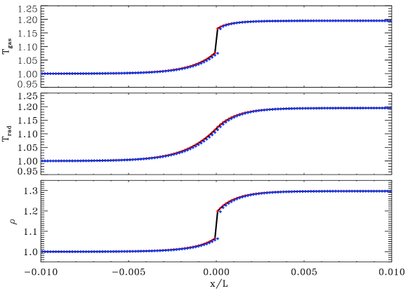
Figure 12.— Profiles of the gas temperature (top), radiation temperature (middle), and density (bottom) versus distance for a radiation modified shock with $\mathcal{M}_{0}=1.2$. The density, gas temperature, and velocity are initialized with a semi-analytic planar shock solution computed using the methods of Lowrie & Edwards (2008) (shown as continuous curves in each plot) while the initial radiation temperature is computed by the RT solver. Quantities are non-dimensionalized as described in Lowrie & Edwards (2008) and discussed in section 5.5. The red crosses indicate the initial conditions for all variables: the fact that the radiation temperature computed by the RT solver initially agrees with the semi-analytic solution confirms the accuracy of the RT solver. The blue crosses show the state of the variables after evolving the shock for $t=L/a_{0}$. There is a small drift in the numerical solution due to the neglect of radiation pressure.

5.5. Radiative Shocks

We now consider the ability of the RT solver to model shocks in the presence of radiation. The physics of radiative shocks has been explored by a number of authors (see Mihalas & Mihalas, 1984, and references therein) and is generally well understood. However, radiating shocks are sufficiently complicated that simple analytic solutions for radiative shocks are generally not available. Fortunately, Lowrie & Edwards (2008) (hereafter LE08) have developed fairly simple, semi-analytic methods for constructing one dimensional planar solutions of radiating shocks, which are suitable for our purposes.

LE08 construct their solutions using a grey non-equilibrium diffusion model of radiation hydrodynamics. Their treatment differs from ours in a few important ways. Rather than solving the RT equation (8) directly, they solve the radiation moment equations with Eddington approximation and assuming a diffusion relation for the radiative flux. They retain a number of velocity dependent terms which are absent in our treatment and include the radiation source term in the material momentum equation (our eq. 2). This allows them to explore the radiation pressure dominated, which is not accessible with the methods discussed here (see, however, JSD12). Hence, our comparisons will be restricted to shock solutions with a low ratio of radiation to gas pressure and modest Mach numbers.

LE08 solve a non-dimensionalized systems of equations with solutions that can be uniquely specified in terms of $\gamma$, $\sigma_{a}$, $\mathcal{P}_{0}$, $\kappa$, and $\mathcal{M}_{0}$ using their notation. Here $\sigma_{a}$ is the non-dimensional absorption cross section, $\mathcal{P}_{0}$ is roughly the ratio of radiation to gas thermal energy in the upstream flow, $\kappa$ is non-dimensional photon diffusivity, and $\mathcal{M}_{0}=v/a_{0}$ is the upstream Mach number. The subscript “0” refers to upstream values in their notation.

Following LE08, we examine solutions with $\gamma=5/3$, $\sigma_{a}=10^{6}$, $\mathcal{P}_{0}=10^{-4}$, and $\kappa=1$. In our notation, these parameters correspond to $E_{\rm rad}=10/9\times 10^{-4}E_{\rm gas}$, $a=1/\sqrt{3}\times 10^{-3}c$, and $\chi^{\rm tot}=\chi^{\rm abs}=1/\sqrt{3}\times 10^{-3}L^{-1}$. Here, $L$ is an arbitrary reference length scale and all variables are evaluated using their asymptotic upstream values.

We construct one-dimensional planar shock solutions following the procedures outlined in LE08 and use the resulting profiles of $\rho$, $v$, and $E_{\rm gas}$ to initialize our one-dimensional simulation domains. Since $\chi^{\rm tot}L\ll 1$, we only simulate the region within a few photon mean-free-paths ($\lambda_{\rm mfp}\sim 1/\chi^{\rm abs}\simeq 0.003L$) of the shock front. Since the semi-analytic solutions rely on the Eddington approximation, we set $n_{\mu}=2$ (i.e. two-stream approximation) for consistency. The radiation field at the boundaries is fixed and assumes that the incoming radiation is in thermodynamic equilibrium with appropriate upstream and downstream asymptotic temperature. We evolve the simulations for a time $\Delta t=L/a$, which is typically a factor of hundred ($\sim L/\lambda_{\rm mfp}$) larger than the sound crossing time of the simulation domain.

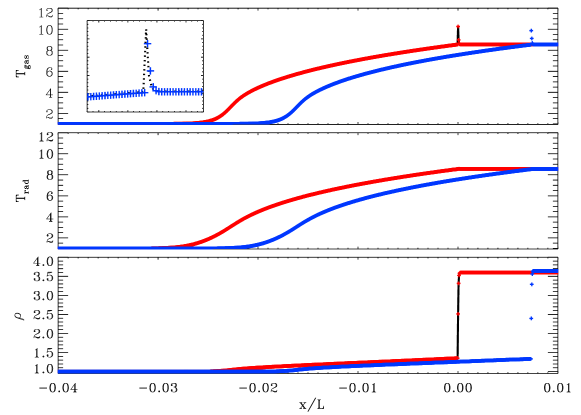
Figure 13.— Same as Figure 12, but for $\mathcal{M}_{0}=5$. The inset in the top panel shows a close-up view of the gas temperature near the shock front at $t=L/a_{0}$ as well as the initial semi-analytic model shifted to the right by an amount $0.0073L$ (the amount the shock front shifts in this timespan) shown as a dotted line. The shock shifts further since radiation pressure is more important at this Mach number, nevertheless the Zeldovich spike (and the overall shock profile) persists.

Figures 12 and 13 show characteristic results for $\mathcal{M}_{0}=1.2$ and 5, respectively. We use 128 and 1024 gridzones for the simulation with $\mathcal{M}_{0}=1.2$ and 5, respectively. We use a larger number for the $\mathcal{M}_{0}=5$ simulation to resolve the narrow Zeldovich spike (Zel’Dovich & Raizer, 1967). We plot the gas temperature $T_{\rm gas}=a^{2}/(\gamma R)$, radiation temperature $T_{\rm rad}=(E_{\rm rad}/a_{R})^{1/4}$, and $\rho$ using the non-dimensional units of LE08. Here, $a_{R}$ is the standard radiation constant and $E_{\rm rad}$ is computed using the RT solver. The fact that $T_{\rm rad}$ computed using the RT solver in the initial shock profile agrees well with the semi-analytic solutions is already an important test of our method. Sufficiently far upstream or downstream of the shock, the gas and radiation are in thermodynamic equilibrium with $T_{\rm gas}=T_{\rm rad}$. Near the shock front, the temperatures deviate, with a radiation precursor upstream of the shock and Zeldovich spikes appearing downstream of the shock for the higher Mach number solutions.

For each plot, we show two sets of curves corresponding to the initial and final profiles. Since we have initialized the simulation with stationary solutions computed in the shock rest frame, the material properties should not evolve with time. However, since our system of equations differ from those used by LE08 to derive their solutions (in particular, we ignore the radiation pressure), our numerical solutions are only approximately stationary. The effects of the terms we have neglected are small for the chosen parameters. Nevertheless, there is a slow but steady drift of the shock location in the downstream direction due to the neglect of the radiation force in the upstream direction. As the Mach number of the flow increases, the radiation force becomes increasingly important and the shock front moves more rapidly in this frame. Even though the position of the shock drifts, the profile changes very little as the radiation source term in the energy equation is still well approximated.

Further tests of radiative shocks are presented in sections 5.2 and 5.3 of JSD12, including calculations that use the RT solver to compute the VET.

5.6. Performance

The added computational cost of using the RT solver is determined by a number of factors and will generally be problem dependent. A useful starting point is a comparison of the computational cost to integrate the MHD equations for one timestep with the cost to perform a single iteration of the RT solver for a single frequency when run on a single processor. For a three dimensional domain with $n_{\mu}=4$ (i.e. 24 total rays) the RT solver requires $\sim 40$% as many operations as the CTU integrator. This is essentially the simplest type of problem that is of practical importance: an LTE grey problem with fixed intensity on the boundaries and an angular discretization that can yield a result beyond the Eddington approximation.

Many problems of interest will be more costly than this because we will need multiple iterations, multiple frequency bins, or higher angular resolution. The total cost of the RT solution scales approximately linearly with the number of frequency groups, total number of angles, or number of iterations, all of which are problem dependent. Even for LTE problems, periodic boundaries or domain decomposition may require multiple iterations. For most problems iteration will continue until the relative change in $S$ (or $J$) is below some prescribed threshold $\delta_{c}$ and the total number of iterations may fluctuate from one timestep to the next, depending on conditions.

For the code tests considered here, which used $\delta_{c}=10^{-5}$, the number of iterations per timestep was $\leq 5$, depending on the problem, with 1-3 iterations being typical. Most of the tests were LTE and iteration was only used to handle boundary conditions. An exception is the uniform non-LTE atmosphere tests that were run with $\gtrsim 1000$ iterations in order to obtain convergence of the absolute error.

We emphasize that Figure 3 is not indicative of the typical number of iterations that need to be performed per timestep, even in highly non-LTE domains. The key point is that this calculation starts from an initial condition that assumes an LTE radiation field everywhere, even though the solution at the surface is far from LTE. As discussed in TF95, the main problem with the ALI methods used here is that they have a rather small spectral radius. Effectively, this means that it takes a rather large number of iterations for errors in the initial condition that span many gridzones to diminish. Since we are computing RT on each timestep, we already have an initial guess that is a reasonable approximation to the correct non-LTE solution. In particular, large (i.e. domain scale) variations in the radiation field are usually already well accounted for by the solution from the previous timestep.

We anticipate that our initial solution of the radiation field before the first timestep may require hundreds to thousands of iterations for highly non-LTE problems (i.e. those with a significant fraction of zones having $\epsilon\ll 1$), but that subsequent timesteps will only require a modest number ($\lesssim 5$) of iterations to obtain relative convergence $|\Delta S|/S\lesssim 10^{-3}$. Our initial work on shearing box simulations (not reported here) supports this expectation, although the number of iterations depends somewhat on just how non-LTE the radiation field becomes. Hayek et al. (2010) report similar numbers of iterations (see their Figure 2) as being typical of their scattering dominated calculations.

A second consideration affecting performance is the maximum timestep that can be used with the operator split update of the total energy described in section 4. The generalized CFL conditions derived in section 5.4 may reduce the timestep when $E_{\rm rad}$ is a significant fraction of $E_{\rm gas}$ or $v\ll c$. For such problems it will be more efficient to use the VET method of JSD12 when feasible.

A third consideration is scalability. Since scaling efficiency will be somewhat machine dependent, we are primarily concerned with assessing how the code performs with RT relative to the (M)HD configuration with no solution of RT. To make the comparison concrete, we study the weak scaling for $32^{3}$ gridzones per core on the SciNet General Purpose Cluster, which consists of eight core nodes made from two 2.53 GHz quad-core Intel Xeon 5500 Nehalem processors. Tests were performed using the Infiniband interconnect. We use a grid aligned radiating linear wave on a three-dimensional domain with $n_{\mu}=4$, $\tau_{0}=1$, and Bo=1 in the radiating case and a slow magnetosonic wave for MHD only calculation. Both tests were performed using the full MHD CTU integrator. We initialize the radiating wave as described in section 5.4, but we only allow a single iteration of the RT solver per timestep. We compute the efficiency by dividing the number of zone cycles/second obtained for a problem run with multiple cores by the number of zone cycles/second for a single core. The resulting scaling with number of cores is nearly identical in the radiating and non-radiating cases, falling to about 75% at 512 cores (64 nodes).

We also find the same scaling efficiency for $n_{\mu}=12$, which is notable because this correspond to a factor of seven increase in the number of specific intensity bins that need to be passed on each iteration. In this case, the increase in communication demands is balanced by the roughly factor of seven increase in the cost of computing the RT solution with more angle bins. These results suggest that the scaling efficiency with the RT solver will tend to follow the non-radiative scaling when they are run on the same platform, as long as the number of iterations remains constant.

The assumption that number of iterations stays fixed is an important caveat. In fact, this assumption will not generally hold since we use iteration to handle subdomain boundaries. To understand this, it is useful to consider two LTE problems: one in which the optical depth across each subdomain is very large and one for which the whole domain is optically thin. In first problem, the radiation field is determined entirely locally and propagation of changes in the radiation field from neighboring subdomains will require only a single iteration. In the second problem, variations in the emissivity on one side of the domain can modify the radiation field on the other. For a cubic array of $N$ subdomains, it could take $\sim N^{1/3}$ iterations to propagate the radiation across the entire domain. This means that scaling efficiency can, in principle, be very problem dependent. For most of the applications of primary interest, the majority of subdomains will be optically thick so increasing the number of subdomains should not significantly increase the number of iterations required. Therefore, scaling efficiency should reasonably consistent with the non-radiating case.

Performance and scaling of the overall VET scheme is discussed in section 7.2 of JSD12.

6. Summary

We have described our implementation of an RT solver in the Athena MHD code. Our module implements a short characteristic method for computing RT on Cartesian, multidimensional simulation domains. The RT equation is solved once each simulation timestep for a computational cost comparable to or less than a single timestep of the MHD integrator for simple (e.g. LTE grey) problems. Since we are focused on astrophysical problems where velocities are slow compared with the speed of light, we drop the time derivative of intensity and the system becomes an integrodifferential equation with no explicit time dependence for the radiation field. The material properties of the flow are evolved using the standard Athena MHD integrators, but with radiative heating and cooling source terms computed from the RT solver. The code solves the RT equation for frequency dependent, absorption and scattering opacities. Non-LTE effects arising from scattering processes are handled with ALI methods. The resulting code is well-suited for non-relativistic astrophysical problems where diffuse emission, rather than bright point sources, constitutes the dominant source of radiation.

We provide a detailed summary of the short characteristics and ALI implementations. We also describe our implementation of an operator split update of the energy equation using a radiation source term computed directly by the RT solver. Alternatively, the RT solver can be used to compute a VET, which can then be input into the integration of the coupled MHD and radiation moment equations. The use of the RT module for this purpose is discussed in a companion paper (JSD12).

We also present results from several test problems, which roughly fall into two classes: tests of the RT solver on static simulation domains, and tests of the coupled RT solver and MHD integrator for time-dependent hydrodynamics simulations. These tests demonstrate the accuracy of the RT solver for multidimensional problems, assess its convergence properties for applications where scattering leads to significant deviations from LTE. They indicate that substantial improvements in accuracy and efficiency may be obtained over alternative methods, such as flux-limited diffusion and Monte Carlo based RT solvers.

The tests also evaluate the accuracy and stability of the MHD integrator when coupled to the RT solver via operator splitting. They verify that the code is generally only first-order accurate for problems where heating or cooling of the fluid by the radiation field is significant. They also illuminate important time step constraints and are useful for assessing the efficiency and accuracy of the code for solving various astrophysical problems.

In particular, we derive a generalized CFL condition, predicated on the need to resolve the non-equilibrium radiation diffusion mode. The requirement to place some limits on timesteps due to rapid radiative relaxation (see e.g. Castor, 2004) are generally acknowledged and implemented in previous work. However, we have not seen any explicit reference to resolving the damping rate of the radiation diffusion mode, which provides a a practical and precise guideline for ensuring numerical stability.

The focus in this work has been on modeling the fluid dynamics and thermodynamics with a self-consistent computation of the radiation field. However, we expect that the ability of the RT solver to provide detailed outputs of the emergent radiation field, such as images, lightcurves, and spectra, may be equally important. Indeed, for some applications the production of such outputs may be the primary motivation for including radiation in the simulation. In principle, the RT solver can be used solely to generate diagnostic outputs, even in simulations without self-consistent feedback of radiation on the material flow, either in real time or via post-processing.

In addition to the simple test problems described here, we are beginning a research program to simulate the local structure of accretion flows (i.e. stratified shearing boxes) with radiative heating and cooling. Applications to radiation dominated environments using the VET method (JSD12) are also underway, and include studies of radiation dominated accretion disks, radiative Rayleigh-Taylor instability, and the radiative driving of cold gas. Applications to extrasolar planets, star forming environments, boundary layers, galactic and accretion disk outflow are also under consideration for future work.

A significant limitation of the RT solver described here is the short-characteristics method’s inability to accurately handle bright points sources. We plan to address this in future work using a hybrid scheme that computes the direct radiation from point sources using the algorithms described in Krumholz et al. (2007b) and models the diffuse emission with RT solver described here.

The source code for our RT solver, test problems and associated documentation will be included in the publicly available version of Athena in the near future. We have endeavored to make the code as user friendly as possible and strongly encourage interested parties to use the code in their own research.

References

- Abel & Wandelt (2002) Abel, T., & Wandelt, B. D. 2002, MNRAS, 330, L53
- Auer (2003) Auer, L. 2003, in Astronomical Society of the Pacific Conference Series, Vol. 288, Stellar Atmosphere Modeling, ed. I. Hubeny, D. Mihalas, & K. Werner, 3–+
- Auer & Paletou (1994) Auer, L. H., & Paletou, F. 1994, A&A, 285, 675
- Blaes et al. (2006) Blaes, O. M., Davis, S. W., Hirose, S., Krolik, J. H., & Stone, J. M. 2006, ApJ, 645, 1402
- Bruenn et al. (2006) Bruenn, S. W., Dirk, C. J., Mezzacappa, A., Hayes, J. C., Blondin, J. M., Hix, W. R., & Messer, O. E. B. 2006, Journal of Physics Conference Series, 46, 393
- Bruls et al. (1999) Bruls, J. H. M. J., Vollmöller, P., & Schüssler, M. 1999, A&A, 348, 233
- Cannon (1973) Cannon, C. J. 1973, ApJ, 185, 621
- Carlson (1963) Carlson, B. G. 1963, Methods in Computational Physics, Vol. 1, Statistical Physics, ed. B. Alder, S. Fernbach, & M. Rotenberg (Academic Press)
- Carlsson (2008) Carlsson, M. 2008, Physica Scripta Volume T, 133, 014012
- Castor (2004) Castor, J. I. 2004, Radiation Hydrodynamics, ed. Castor, J. I.
- Chandrasekhar (1960) Chandrasekhar, S. 1960, Radiative transfer, ed. Chandrasekhar, S.
- Commerçon et al. (2011) Commerçon, B., Teyssier, R., Audit, E., Hennebelle, P., & Chabrier, G. 2011, A&A, 529, A35+
- Davis et al. (2009) Davis, S. W., Blaes, O. M., Hirose, S., & Krolik, J. H. 2009, ApJ, 703, 569
- Densmore et al. (2007) Densmore, J. D., Urbatsch, T. J., Evans, T. M., & Buksas, M. W. 2007, Journal of Computational Physics, 222, 485
- Feautrier (1964) Feautrier, P. 1964, Comptes Rendus Academie des Sciences (serie non specifiee), 258, 3189
- Finlator et al. (2009) Finlator, K., Özel, F., Davé, R., & Oppenheimer, B. D. 2009, MNRAS, 400, 1049
- Gardiner & Stone (2008) Gardiner, T. A., & Stone, J. M. 2008, Journal of Computational Physics, 227, 4123
- Gittings et al. (2008) Gittings, M., et al. 2008, Computational Science and Discovery, 1, 015005
- González et al. (2007) González, M., Audit, E., & Huynh, P. 2007, A&A, 464, 429
- Hayek et al. (2010) Hayek, W., Asplund, M., Carlsson, M., Trampedach, R., Collet, R., Gudiksen, B. V., Hansteen, V. H., & Leenaarts, J. 2010, A&A, 517, A49+
- Hayes & Norman (2003) Hayes, J. C., & Norman, M. L. 2003, ApJS, 147, 197
- Hayes et al. (2006) Hayes, J. C., Norman, M. L., Fiedler, R. A., Bordner, J. O., Li, P. S., Clark, S. E., ud-Doula, A., & Mac Low, M.-M. 2006, ApJS, 165, 188
- Heinemann et al. (2006) Heinemann, T., Dobler, W., Nordlund, Å., & Brandenburg, A. 2006, A&A, 448, 731
- Heinemann et al. (2007) Heinemann, T., Nordlund, Å., Scharmer, G. B., & Spruit, H. C. 2007, ApJ, 669, 1390
- Hirose et al. (2006) Hirose, S., Krolik, J. H., & Stone, J. M. 2006, ApJ, 640, 901
- Hubeny (2003) Hubeny, I. 2003, in Astronomical Society of the Pacific Conference Series, Vol. 288, Stellar Atmosphere Modeling, ed. I. Hubeny, D. Mihalas, & K. Werner, 17–+
- Hubeny & Burrows (2007) Hubeny, I., & Burrows, A. 2007, ApJ, 659, 1458
- Jiang et al. (2012) Jiang, Y.-F., Stone, J. M., & Davis, S. W., ApJS, submitted (JSD12)
- Krumholz et al. (2007a) Krumholz, M. R., Klein, R. I., McKee, C. F., & Bolstad, J. 2007a, ApJ, 667, 626
- Krumholz et al. (2007b) Krumholz, M. R., Stone, J. M., & Gardiner, T. A. 2007b, ApJ, 671, 518
- Kunasz & Auer (1988) Kunasz, P., & Auer, L. H. 1988, J. Quant. Spec. Radiat. Transf., 39, 67
- Levermore & Pomraning (1981) Levermore, C. D., & Pomraning, G. C. 1981, ApJ, 248, 321
- Lowrie & Edwards (2008) Lowrie, R. B., & Edwards, J. D. 2008, Shock Waves, 18, 129
- Lowrie et al. (1999) Lowrie, R. B., Morel, J. E., & Hittinger, J. A. 1999, ApJ, 521, 432
- Mellema et al. (2006) Mellema, G., Iliev, I. T., Alvarez, M. A., & Shapiro, P. R. 2006, New A, 11, 374
- Mihalas et al. (1978) Mihalas, D., Auer, L. H., & Mihalas, B. R. 1978, ApJ, 220, 1001
- Mihalas & Klein (1982) Mihalas, D., & Klein, R. I. 1982, Journal of Computational Physics, 46, 97
- Mihalas & Mihalas (1984) Mihalas, D., & Mihalas, B. W. 1984, Foundations of radiation hydrodynamics, ed. Mihalas, D. & Mihalas, B. W.
- Nordlund (1982) Nordlund, A. 1982, A&A, 107, 1
- Olson et al. (1986) Olson, G. L., Auer, L. H., & Buchler, J. R. 1986, J. Quant. Spec. Radiat. Transf., 35, 431
- Olson & Kunasz (1987) Olson, G. L., & Kunasz, P. B. 1987, J. Quant. Spec. Radiat. Transf., 38, 325
- Reynolds et al. (2009) Reynolds, D. R., Hayes, J. C., Paschos, P., & Norman, M. L. 2009, Journal of Computational Physics, 228, 6833
- Rijkhorst et al. (2006) Rijkhorst, E.-J., Plewa, T., Dubey, A., & Mellema, G. 2006, A&A, 452, 907
- Rybicki & Hummer (1991) Rybicki, G. B., & Hummer, D. G. 1991, A&A, 245, 171
- Sekora & Stone (2010) Sekora, M. D., & Stone, J. M. 2010, Journal of Computational Physics, 229, 6819
- Skartlien (2000) Skartlien, R. 2000, ApJ, 536, 465
- Stein & Nordlund (1998) Stein, R. F., & Nordlund, A. 1998, ApJ, 499, 914
- Stein & Spiegel (1967) Stein, R. F., & Spiegel, E. A. 1967, Acoustical Society of America Journal, 42, 866
- Stone & Gardiner (2009) Stone, J. M., & Gardiner, T. 2009, New A, 14, 139
- Stone et al. (2008) Stone, J. M., Gardiner, T. A., Teuben, P., Hawley, J. F., & Simon, J. B. 2008, ApJS, 178, 137
- Stone et al. (1992) Stone, J. M., Mihalas, D., & Norman, M. L. 1992, ApJS, 80, 819
- Swesty & Myra (2009) Swesty, F. D., & Myra, E. S. 2009, ApJS, 181, 1
- Trujillo Bueno & Fabiani Bendicho (1995) Trujillo Bueno, J., & Fabiani Bendicho, P. 1995, ApJ, 455, 646
- Turner & Stone (2001) Turner, N. J., & Stone, J. M. 2001, ApJS, 135, 95
- van der Holst et al. (2011) van der Holst, B., et al. 2011, ApJS, 194, 23
- van Noort et al. (2002) van Noort, M., Hubeny, I., & Lanz, T. 2002, ApJ, 568, 1066
- Vögler et al. (2005) Vögler, A., Shelyag, S., Schüssler, M., Cattaneo, F., Emonet, T., & Linde, T. 2005, A&A, 429, 335
- Whalen & Norman (2006) Whalen, D., & Norman, M. L. 2006, ApJS, 162, 281
- Zel’Dovich & Raizer (1967) Zel’Dovich, Y. B., & Raizer, Y. P. 1967, Physics of shock waves and high-temperature hydrodynamic phenomena, ed. Zel’Dovich, Y. B. & Raizer, Y. P.
- Zhang et al. (2011) Zhang, W., Howell, L., Almgren, A., Burrows, A., & Bell, J. 2011, ApJS, 196, 20