Multi-sensor Information Processing using Prediction Market-based Belief Aggregation

We consider the problem of information fusion from multiple sensors of different types with the objective of improving the confidence of inference tasks, such as object classification, performed from the data collected by the sensors. We propose a novel technique based on distributed belief aggregation using a multi-agent prediction market to solve this information fusion problem. To monitor the improvement in the confidence of the object classification as well as to dis-incentivize agents from misreporting information, we have introduced a market maker that rewards the agents instantaneously as well as at the end of the inference task, based on the quality of the submitted reports. We have implemented the market maker’s reward calculation in the form of a scoring rule and have shown analytically that it incentivizes truthful revelation or accurate reporting by each agent. We have experimentally verified our technique for multi-sensor information fusion for an automated landmine detection scenario. Our experimental results show that, for identical data distributions and settings, using our information aggregation technique increases the accuracy of object classification favorably as compared to two other commonly used techniques for information fusion for landmine detection.

1 Introduction

Information fusion from multiple sensors has been a central research topic in sensor-based systems [17] and recently several multi-agent techniques [16] have been proposed to address this problem. Most of the solutions for multi-sensor information fusion and processing are based on Bayesian inference techniques [8, 13, 15]. While such techniques have been shown to be very effective, we investigate a complimentary problem where sensors can behave in a self-interested manner. Such self-interested behavior can be motivated by malicious nodes that might have been planted into the system to subvert its operation, or, by normal sensor nodes attempting to give an illusion of efficient performance when they do not have enough resources (e.g., battery power) to perform accurate measurements. To address this problem, we describe a market-based aggregation technique called a prediction market for multi-sensor information fusion that includes a utility driven mechanism to motivate each sensor, through its associated agent, to reveal accurate reports.

To motivate our problem we describe a distributed automated landmine detection scenario used for humanitarian demining. An environment contains different buried objects, some of which could potentially be landmines. A set of robots, each equipped with one of three types of landmine detection sensor such as a metal detector (MD), or a ground penetrating radar (GPR) or an infra-red (IR) heat sensor, are deployed into this environment. Each robot is capable of perceiving certain features of a buried object through its sensor such as the object’s metal content, area, burial depth, etc. However, the sensors give noisy readings for each perceived feature depending on the characteristics of the object as well as on the characteristics of the environment (e.g., moisture content, ambient temperature, sunlight, etc.). Consequently, a sensor that works well in one scenario, fails to detect landmines in a different scenario, and, instead of a single sensor, multiple sensors of different types, possibly with different detection accuracies can detect landmines with higher certainty [5]. Within this scenario, the central question that we intend to answer is: given an initial set of reports about the features of a buried object, what is a suitable set (number and type) of sensors to deploy over a certain time window to the object, so that, over this time window, the fused information from the different sensors successively reduces the uncertainty in determining the object’s type.

Our work in this paper is based on the insight that the scenario illustrated above, of fusing information from multiple sources to predict the outcome of an initially unknown object, is analogous to the problem of aggregating the beliefs of different humans to forecast the outcome of an initially unknown event. Such forecasting is frequently encountered in many problems such as predicting the outcome of geo-political events, predicting the outcome of financial instruments like stocks, etc. Recently, a market-based model called prediction market has been shown to be very successful in aiding humans with such predictions and with decision-making [1, 2, 14, 18]. Building on these models, in this paper, we describe a multi-agent prediction market for multi-sensor information fusion. Besides being an efficient aggregation mechanism, using prediction markets gives us several useful features - a mathematical formulation called a scoring rule that deters malicious sensors from misreporting information, a regression-based belief update mechanism for the sensor agents for incorporating the aggregated beliefs (or information estimates) of other sensors into their own calculation, and the ability to incorporate an autonomous decision maker that uses expert-level domain knowledge to make utility maximizing decisions to deploy additional sensors appropriately to improve the detection of an object. Our experimental results illustrated with a landmine detection scenario while using identical data distributions and settings, show that the information fusion performed using our technique reduces the root mean squared error by $5-13\%$ as compared to a previously studied technique for landmine data fusion using the Dempster-Shafer theory [10] and by $3-8\%$ using distributed data fusion technique [9].

2 Related Work

Multi-agent Information Fusion. Multi-agent systems have been used to solve various sensor network related problems and an excellent overview is given in [16]. In the direction of multi-sensor information processing, significant works include the use of particle filters[15], distributed data fusion (DDF) architecture along with its extension, the Bayesian DDF [8, 9], Gaussian processes [13] and mobile agent-based information fusion [19]. For most of the application domains described in these works such as water-tide height measurement, wind speed measurement, robot tracking and localization, etc., self-interested behavior by the sensors is not considered a crucial problem. For our illustrated application domain of landmine detection, decision-level fusion techniques have been reported to be amenable for scenarios where the sensor types are different from each other, and, non-statistical decision-level fusion techniques, such as Dempster-Shafer theory [10], fuzzy logic[3], and rule-based fusion techniques [5] have been reported to generalize well. However, in contrast to our work, these techniques assume that sensors are fully cooperative and never behave self-interestedly by misreporting information. In [12], the authors have observed that most sensor-based information aggregation techniques either do not consider malicious behavior or use high-overhead, cryptographic techniques to combat it. To deter false reports by sensor nodes in a data aggregation setting, they propose various lower overhead reputation-based schemes. Our prediction market-based information aggregation technique is complimentary to such reputation-based aggregation techniques.

Decision-Making using Prediction Markets. A prediction market is a market-based aggregation mechanism that is used to combine the opinions on the outcome of a future, real-world event from different people, called the market’s traders and forecast the event’s possible outcome based on their aggregated opinion. Recently, multi-agent systems have been used [1, 7, 14] to analyze the operation of prediction markets, where the behaviors of the market’s participants are implemented as automated software agents. The seminal work on prediction market analysis [18] has shown that the mean belief values of individual traders about the outcome of a future event corresponds to the event’s market price. The basic operation rules of a prediction market are similar to those of a continuous double auction, with the role of the auctioneer being taken up by an entity called the market maker that runs the prediction market. Hanson [6] developed a mechanism, called a scoring rule, that can be used by market makers to reward traders for making and improving a prediction about the outcome of an event, and, showed that if a scoring rule is proper or incentive compatible, then it can serve as an automated market maker. Recently, authors in [2, 14] have theoretically analyzed the properties of prediction markets used for decision making. In [14], the authors analyzed the problem of a decision maker manipulating a prediction market and proposed a family of scoring rules to address the problem. In [2], the authors extended this work by allowing randomized decision rules, considering multiple possible outcomes and providing a simple test to determine whether the scoring rule is proper for an arbitrary decision rule-scoring rule pair. In this paper, we use a prediction market for decision making, but in contrast to previous works we consider that the decision maker can make multiple, possibly improved decisions over an event’s duration, and, the outcome of an event is decided independently, outside the market, and not influenced by the decision maker’s decisions. Another contribution our paper makes is a new, proper scoring rule, called the payment function, that incentivizes agents to submit truthful reports.

3 Problem Formulation

Let $L$ be a set of objects. Each object has certain features that determine its type. We assume that there are $f$ different features and $m$ different object types. Let $\Phi=\{\phi_{1},\phi_{2},...,\phi_{f}\}$ denote the set of object features and $\Theta=\{\theta_{1},\theta_{2},...,\theta_{m}\}$ denote the set of object types. The features of an object $l\in L$ is denoted by $l_{\Phi}\subseteq\Phi$ and its type is denoted by $l_{\theta}\in\Theta$. As illustrated in the example given in Section 1, $l_{\Phi}$ can be perceived, albeit with measurement errors, through sensors, and, our objective is to determine $l_{\theta}$ as accurately as possible from the perceived but noisy values of $l_{\Phi}$. Let $\Delta(\Theta)=\{(\delta(\theta_{1}),\delta(\theta_{2}),...,\delta(\theta_{m})):\delta(\theta_{i})\in[0,1],\sum_{i=1}^{m}\delta(\theta_{i})=1\}$, denote the set of probability distributions over the different object types. For convenience of analysis, we assume that when the actual type of object $l$, $l_{\theta}=\theta_{j}$, its (scalar) type is expanded into a $m$-dimensional probability vector using the function $vec:\Theta\rightarrow[0,1]^{m}:vec_{j}=1,vec_{i\neq j}=0$, which has $1$ as its $j$-th component corresponding to $l$’s type $\theta_{j}$ and $0$ for all other components.

Let $A$ denote a set of agents (sensors) and $A^{t,l}_{rep}\subseteq A$ denote the subset of agents that are able to perceive the object $l$’s features on their sensors at time $t$. Based on the perceived object features, agent $a\in A_{rep}^{t,l}$ at time $t$ reports a belief as a probability distribution over the set of object types, which is denoted as $\mathbf{b}^{a,t,l}\in\Delta(\Theta)$. The beliefs of all the agents are combined into a composite belief, $\mathbf{B}^{t,l}=Agg_{a\in A_{rep}^{t,l}}(\mathbf{b}^{a,t,l})$, and let $\hat{\Theta}^{t,l}:\mathbf{B}^{t,l}\rightarrow\Delta(\Theta)$ denote a function that computes a probability distribution over object types based on the aggregated agent beliefs. Within this setting we formulate the object classification problem as a decision making problem in the following manner: given an object $l$ and an initial aggregated belief $\mathbf{B}^{t,l}$ calculated from one or more agent reports for that object, determine a set of additional agents (sensors) that need to be deployed at object $l$ such that the following constraint is satisfied:

$$\min\,RMSE\left(\hat{\Theta}^{t,l},vec(l_{\theta})\right),\quad\mbox{for}\quad t=1,2,....T$$ (1)

where $T$ is the time window for classifying an object $l$ and RMSE is the root mean square error given by $RMSE(\mathbf{x},\mathbf{y})=\frac{\mid\mid x-y\mid\mid}{\sqrt{m}}$. In other words, at every time step $t$, the decision maker tries to select a subset of agents such that the root mean square error (RMSE) between the estimated type of object $l$ and its actual type is successively minimized.

The major components of the object classification problem described above consists of two parts: integrating the reports from the different sensors and making sensor deployment decisions based on those reports so that the objective function given in Equation 1 is satisfied. To address the first part, we have used distributed information aggregation with a multi-agent prediction market, while for the latter we have used an expected utility maximizing decision-making framework. A schematic showing the different components of our system and their interactions is shown in Figure 1 and explained in the following sections.

Figure 1: The different components of the prediction market for decision making and the interactions between them.

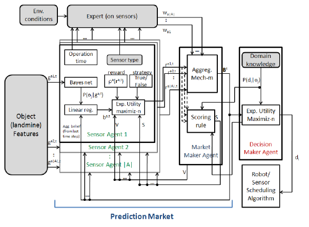
3.1 Sensor Agents

As mentioned in Section 1, there is a set of robots in the scenario and each robot has an on-board sensor for analyzing the objects in the scenario. Different robots can have different types of sensors and sensors of the same type can have different degrees of accuracy determined by their cost. Every sensor is associated with a software agent that runs on-board the robot and performs calculations related to the data sensed by the robot’s sensor. In the rest of the paper, we have used the terms sensor and agent interchangeably. For the ease of notation, we drop the subscript $l$ corresponding to an object for the rest of this section. When an object is within the sensing range of a sensor (agent) $a$ at time $t$, the sensor observes the object’s features and its agent receives this observation in the form of an information signal $g^{a,t}=<g_{1},...,g_{f}>$ that is drawn from the space of information signals $G\subseteq\Delta(\Theta)$. The conditional probability distribution of object type $\theta_{j}$ given an information signal $g\in G$, $P(\theta_{j}|g):G\rightarrow[0,1]$, is constructed using domain knowledge [3, 10, 11] within a Bayesian network and is made available to each agent. Agent $a$ then updates its belief distribution $\mathbf{b}^{a,t}$ using the following equation:

$$\mathbf{b}^{a,t}=w_{bel}\cdot\mathbf{P}(\Theta|g^{a,t})+(1-w_{bel})\cdot\mathbf{B}^{t},$$ (2)

where $\mathbf{B}^{t}$ is the belief value vector aggregated from all sensor reports.

Agent Rewards. Agents behave in a self-interested manner to ensure that they give their ‘best’ report using their available resources including sensor, battery power, etc. However, some agents can behave maliciously, either being planted or compromised to infiltrate the system and subvert the object classification process, or, they might be trying to give an illusion of being efficient when they do not have sufficient resources to give an accurate report. An agent $a$ that submits a report at time $t$, uses its belief distribution $\mathbf{b}^{a,t}$ to calculate the report $\mathbf{r}^{a,t}=<r_{1}^{a,t},...,r_{m}^{a,t}>\in\Delta(\Theta)$. An agent can have two strategies to make this report - truthful or malicious. If the agent is truthful, its report corresponds to its belief, i.e., $\mathbf{r}^{a,t}=\mathbf{b}^{a,t}$. But if it is malicious, it manipulates its report to reveal an inaccurate belief. Each agent $a$ can update its report $\mathbf{r}^{a,t}$ within the time window $T$ by obtaining new measurements from the object and using Equation 2 to update its belief. The report from an agent $a$ at time $t$ is analyzed by a human or agent expert [10] to assign a weight $w^{a,t}$ depending on the current environment conditions and agent $a$’s sensor type’s accuracy under those environment conditions (e.g., rainy weather reduces the weight assigned to the measurement from an IR heat sensor, or, soil that is high in metal content reduces the weight assigned to the measurement from an metal detector).

To motivate an agent to submit reports, an agent $a$ gets an instantaneous reward, $\rho^{a,t}$, from the market maker for the report $\mathbf{r}^{a,t}$ it submits at time $t$, corresponding to its instantaneous utility, which is given by the following equation:

$$\rho^{a,t}=V(n^{t^{\prime}=1..t})-C^{a}(\mathbf{r}^{a,t}),$$ (3)

where $V(n^{t^{\prime}=1..t})$ is the value for making a report with $n^{t^{\prime}=1..t}$ being the number of times the agent $a$ submitted a report up to time $t$, and, $C^{a}(\mathbf{r}^{a,t})$ is the cost of making report $\mathbf{r}^{a,t}$ for agent $a$ based on the robot’s expended time, battery power, etc. We denote the agent’s value for each report $V(n^{t^{\prime}=1..t})$ as a constant-valued function up to a certain threshold and a linearly decreasing function thereafter, to de-incentivize agents from making a large number of reports. Agent $a$’s value function is given by the following equation:

$$V(n^{t^{\prime}=1..t})=\left\{\begin{array}[]{ll}\nu&,n^{t^{\prime}=1..t}\leq n^{threshold}\\ \frac{\nu(n^{t^{\prime}=1..t}-n^{max})}{(n^{threshold}-n^{max})}&,otherwise\end{array}\right.$$

where $\nu\in\mathbb{Z^{+}}$, is a constant value that $a$ gets by submitting reports up to a threshold, $n^{threshold}$ is the threshold corresponding to the number of reports $a$ can submit before its report’s value starts decreasing, and, $n^{max}$ is the maximum number of reports agent $a$ can submit before $V$ becomes negative. Finally, to determine its strategy while submitting its report, an agent selects the strategy that maximizes its expected utility obtained from its cumulative reward given by Equation 3 plus an expected value of its final reward payment if it continues making similar reports up to the object’s time window $T$.

3.2 Decision Maker Agent

The decision maker agent’s task is to use the composite belief about an object’s type, $\mathbf{B}^{t}$, given by the prediction market, and take actions to deploy additional robots(sensors) based on the value of the objective function given in Equation 1. Let $AC$ denote a set of possible actions corresponding to deploying a certain number of robots, and $D=\{d_{1},...d_{h}\}:d_{i}\in Ac\subseteq AC$ denote the decision set of the decision maker. The decision function of the decision maker is given by $dec:\Delta(\Theta)\rightarrow D$. Let $\mathbf{u}^{dec}_{j}\in\mathbb{R}^{m}$ be the utility that the decision maker receives by determining an object to be of type $\theta_{j}$ and let $P(d_{i}|\theta_{j})$ be the probability that the decision maker makes decision $d_{i}\in D$ given object type $\theta_{j}$. $P(d_{i}|\theta_{j})$ and $\mathbf{u}^{dec}_{j}$ are constructed using domain knowledge [3, 11, 10]. Given the aggregated belief distribution $\mathbf{B}^{t}$ at time $t$, the expected utility to the decision maker for taking decision $d_{i}$ at time $t$ is then $EU^{dec}(d_{i},\mathbf{B}^{t})=\sum_{j=1}^{m}P(d_{i}|\theta_{j})\cdot\mathbf{u}^{dec}_{j}\cdot\mathbf{B}^{t}$. The decision that the decision maker takes at time $t$, also called its decision rule, is the one that maximizes its expected utility and is given by: $d^{t}=\arg\max_{d_{i}}EU^{dec}(d_{i},\mathbf{B}^{t})$.

3.3 Prediction Market

A conventional prediction market uses the aggregated beliefs of the market’s participants or traders about the outcome of a future event, to predict the event’s outcome. The outcome of an event is represented as a binary variable (event happens/does not happen). The traders observe information related to the event and report their beliefs, as probabilities about the event’s outcome. The market maker aggregates the traders’ beliefs and uses a scoring rule to determine a payment or payoff that will be received by each reporting trader. In our multi-agent prediction market, traders correspond to sensor agents, the market maker agent automates the calculations on behalf of the conventional market maker, and, an event in the conventional market corresponds to identifying the type of a detected object. The time window $T$ over which an object is sensed is called the duration of the object in the market. This time window is divided into discrete time steps, $t=1,2...T$. During each time step, each sensor agent observing the object submits a report about the object’s type to the market maker agent. The market maker agent performs two functions with these reports. First, at each time step $t$, it aggregates the agent reports into an aggregated belief about the object, $\mathbf{B}^{t}\in\Delta(\Theta)$. Secondly, it calculates and distributes payments for the sensor agents. It pays an immediate but nominal reward to each agent for its report at time step $t$ using Equation 3. Finally, at the end of the object’s time window $T$, the market maker also gives a larger payoff to each agent that contributed towards classifying the object’s type. The calculations and analysis related to these two functions of the market maker agent are described in the following sections.

Final Payoff Calculation. The payoff calculation for a sensor agent is performed by the market maker using a decision scoring rule at the end of the object’s time window. A decision scoring rule [2] is defined as any real valued function that takes the agents’ reported beliefs, the realized outcome and the decisions made by the decision maker as input, and produces a payoff for the agent for its reported beliefs, i.e. $S:\Delta(\Theta)\times\Theta\times D\longrightarrow\mathbb{R}$. We design a scoring rule for decision making that is based on how much agent $a$’s final report helped the decision maker to make the right decisions throughout the duration of the prediction market and by how close the agent $a$’s final report is to actual object type. Our proposed scoring rule for decision making given that object’s true type is $\theta_{j}$ is given in Equation 4:

$$S(r_{j}^{a,t},d^{[1:t]},\theta_{j})=\varpi(d^{[1:t]},\theta_{j})log\left(r_{j}^{a,t}\right),$$ (4)

where, $r_{j}^{a,t}$ is the reported belief that agent $a$ submitted at time $t$ for object type $\theta_{j}$, $d^{[1:t]}$ is the set consisting of all the decisions that the decision maker took related to the object up to the current time $t$, $\theta_{j}$ is the object’s true type that was revealed at the end the object’s time window, $log\left(r_{j}^{a,t}\right)$ measures the goodness of the report at time $t$ relative to the true object type $\theta_{j}$, and, $\varpi(d^{[1:t]},\theta_{j})$ is the weight, representing how good all the decisions the decision maker took up to time $t$ were compared to the true object type $\theta_{j}$. $\varpi(d^{[1:t]},\theta_{j})$ is determined by the decision maker and made available to the agents through the market maker. We assume that $\varpi(d^{[1:t]},\theta_{j})=\sum_{i=1}^{t}P(d_{i}\mid\theta_{j})\cdot\mathbf{u}_{j}^{dec}$, which gives the expected utility of the decision maker agent for making decision $i$ when the true type of the object is $\theta_{j}$.

Aggregation. Since a sensor agent gets paid both through its immediate rewards for making reports during the object’s time window and through the scoring rule function for decision making at the end of the object’s time window, we define the total payment that the agent has received by the end of the object’s time window as a payment function.

Definition 1.

A function $\Psi(\mathbf{r}^{a,t},d^{[1:t]},\theta_{j},n^{t^{\prime}=1..t})$ is called a payment function if each agent $a$’s total received payment at the end of the object’s time window (when $t=T$) is

$$\Psi(\mathbf{r}^{a,t},d^{[1:t]},\theta_{j},n^{t^{\prime}=1..t})=\sum_{k=1}^{t}\rho^{a,k}+S(r_{j}^{a,t},d^{[1:t]},\theta_{j})\\$$ (5)

where $\rho^{a,k}$, $S(r_{j}^{a,t},d^{[1:t]},\theta_{j})$ and their components are defined as in Equations 3 and 4.

Let $\Psi^{ave}$ denote a weighted average of the payment function in Equation 5 over all the reporting agents, using the report-weights assigned by the expert in Section 3.1, as given below:

$$\Psi^{ave}(\mathbf{r}^{A_{rep}^{t},t},d^{[1:t]},\theta_{j},n^{A_{rep}^{t},t}) =\sum_{k=1}^{t}\sum_{a\in A^{t}_{rep}}w^{a,k}\rho^{a,k}$$ (6)

$$+\varpi(d^{[1:t]},\theta_{j})\sum_{a\in A^{t}_{rep}}w^{a,t}log\left(r_{j}^{a,t}\right),$$

where $A_{rep}^{t}$ is the subset of agents that are able to perceive object feature at time $t$ and $w^{a,k}$ is the weight assigned to agent $a$ at time $k$ by the expert. To calculate an aggregated belief value in a prediction market, Hanson [6] used the generalized inverse function of the scoring rule. Likewise, we calculate the aggregated belief for our market maker agent by taking the generalized inverse of the average payment function given in Equation 3.3:

$$B^{t}_{j} =Agg_{a\in A_{rep}^{t}}(\mathbf{b}^{a,t})$$ (7)

$$=\frac{\frac{exp\left(\Psi^{ave}-\sum_{k=1}^{t}\sum_{a\in A^{t}_{rep}}w^{a,k}\rho^{a,k}\right)}{\varpi(d^{[1:t]},\theta_{j})}}{\frac{\sum_{\theta_{j}=\theta_{1}}^{\theta_{m}}exp\left(\Psi^{ave}-\sum_{k=1}^{t}\sum_{a\in A^{t}_{rep}}w^{a,k}\rho^{a,k}\right)}{\varpi(d^{[1:t]},\theta_{j})}}$$ (8)

where $B^{t}_{j}\in\mathbf{B}^{t}$ is the $j$-th component of the aggregated belief for object type $\theta_{j}$. The aggregated belief vector, $\mathbf{B}^{t}$, calculated by the market maker agent is sent to the decision maker agent so that it can calculate its expected utility given in Section 3.2, as well as, sent back to each sensor agent that reported the object’s type till time step $t$, so that the agent can refine its future reports, if any, using this aggregate of the reports from other agents.

4 Payment function: Properties
and Characteristics

In this section we first show that the payment function is proper, or incentive compatible. Then we show that when the market maker uses this payment function to reward each agent for its reported beliefs, reporting beliefs truthfully is the optimal strategy for each agent.

We can characterize a proper payment function similar to a proper scoring rule.

Definition 2.

A payment function $\Psi$ is proper, or incentive compatible, if

$$\Psi(\mathbf{b^{a,t}},d^{[1:t]},\theta_{j},n^{t^{\prime}=1..t})\geq\Psi(\mathbf{r^{a,t}},d^{[1:t]},\theta_{j},n^{t^{\prime}=1..t}),$$ (9)

$\forall\mathbf{b^{a,t}},\mathbf{r^{a,t}}\in\Delta(O).$

$\Psi$ is strictly proper if Equation 9 holds with equality, i.e., iff $\mathbf{b^{a,t}}=\mathbf{r^{a,t}}$.

Payment functions can be shown to be proper by representing them using convex functions [2, 4]. To show that our payment function in Equation 5 is proper, we characterize it in terms of a convex function, as shown below:

Theorem 1.

A payment function $\Psi$ is proper for decision making if

$$\Psi(\mathbf{r^{a,t}},d^{[1:t]},\theta_{j},n^{t^{\prime}=1..t})=G(\mathbf{r^{a,t}})-G^{\prime}(\mathbf{r^{a,t}})\cdot(\mathbf{r^{a,t}})+\frac{G^{\prime}_{i,j}(\mathbf{r^{a,t}})}{P(d_{i}|\theta_{j})},$$ (10)

where $G(\mathbf{r^{a,t}})$ is a convex function and $G^{\prime}(\mathbf{r^{a,t}})$ is a subgradient of $G$ at point $\mathbf{r^{a,t}}$ and $P(d_{i}|\theta_{j})>0$.

Proof.

Consider a payment function $\Psi$ satisfying Equation 10. We will show that $\Psi$ must be proper for decision making. We will drop the agent and time subscripts in this proof, and also we will write $\Psi(\mathbf{r},d^{[1:t]})$ (or its element $\Psi(r_{j},d_{i}|\theta_{j})$) instead of full $\Psi(\mathbf{r^{a,t}},d^{[1:t]},\theta_{j},n^{t^{\prime}=1..t})$.

$$EU(\mathbf{b},\mathbf{b}) =\sum_{i=1}^{h}\sum_{j=1}^{m}P(d_{i}|\theta_{j})b_{j}\Psi(b_{j},d_{i}|\theta_{j})$$

$$=\sum_{i=1}^{h}\sum_{j=1}^{m}P(d_{i})b_{j}\left(G(\mathbf{b})-G^{\prime}(\mathbf{b})\cdot\mathbf{b}+\frac{G^{\prime}_{i,j}(\mathbf{b})}{P(d_{i}|\theta_{j})}\right)$$

$$=G(\mathbf{b})-G^{\prime}(\mathbf{b})\cdot\mathbf{b}+\sum_{i=1}^{h}\sum_{j=1}^{m}G^{\prime}_{i,j}(\mathbf{b})b_{j}$$

$$=G(\mathbf{b})-G^{\prime}(\mathbf{b})\cdot\mathbf{b}+G^{\prime}(\mathbf{b})\cdot\mathbf{b}=G(\mathbf{b}).$$

Since $G$ is convex and $G^{\prime}$ is its subgradient, we have

$$EU(\mathbf{b},\mathbf{r}) =\sum_{i=1}^{h}\sum_{j=1}^{m}P(d_{i}|\theta_{j})b_{j}\Psi(r_{j},d_{i}|\theta_{j})$$

$$=\sum_{i=1}^{h}\sum_{j=1}^{m}P(d_{i}|\theta_{j})b_{j}\left(G(\mathbf{r})-G^{\prime}(\mathbf{r})\cdot\mathbf{r}+\frac{G^{\prime}_{i,j}(\mathbf{r})}{P(d_{i}|\theta_{j})}\right)$$

$$=G(\mathbf{r})-G^{\prime}(\mathbf{r})(\mathbf{b}-\mathbf{r})$$

$$\leq G(\mathbf{b})=EU(\mathbf{b},\mathbf{b}).$$

Thus, $\Psi$ is a proper payment function for decision making. $\Psi$ is strictly proper payment function and the inequality is strict if $G$ is a strictly convex function. ∎

Proposition 1.

The payment function given in Equation 5 is proper.

Proof.

Let $G(\mathbf{b})=EU(\mathbf{b},\mathbf{b})$ and
$G^{\prime}_{i,j}(\mathbf{b})=P(d_{i}|\theta_{j})\Psi(\mathbf{b},d^{[1:t]},\theta_{j},n^{t^{\prime}=1..t})$. Then we can write the payment function as

$$\Psi(\mathbf{b},d^{[1:t]},\theta_{j},n^{t^{\prime}=1..t}) =\sum_{i=1}^{h}\sum_{j=1}^{m}P(d_{i}|\theta_{j})b_{j}\Psi(\mathbf{b},d^{[1:t]},\theta_{j},n^{t^{\prime}=1..t})$$

$$-\mathbf{b}\cdot\sum_{i=1}^{h}\sum_{j=1}^{m}P(d_{i}|\theta_{j})\Psi(\mathbf{b},d^{[1:t]},\theta_{j},n^{t^{\prime}=1..t})$$

$$+\frac{\Psi(\mathbf{b},d^{[1:t]},\theta_{j},n^{t^{\prime}=1..t})\cdot P(d_{i}|\theta_{j})}{P(d_{i}|\theta_{j})}$$

$$=\Psi(\mathbf{b},d^{[1:t]},\theta_{j},n^{t^{\prime}=1..t}).$$

We can clearly see that the payment function can be written in the form given in Equation 10 from Theorem 1. Therefore, the payment function $\Psi$ given in Equation 5 is a proper payment function. ∎

Agent Reporting Strategy. Assume that agent $a$’s report at time $t$ is its final report, then its utility function can be written as $u_{j}^{a,t}=\sum_{k=1}^{t}\rho^{a,k}+S(r_{j}^{a,t},d^{[1:t]},\theta_{j})$. Then, agent $a$’s expected utility for object type $\theta_{j}$ given its reported belief for object type $\theta_{j}$, $r_{j}^{a,t}$, and its true belief about object type $\theta_{j}$, $b_{j}^{a,t}$ at time $t$ is

$$EU_{j}^{a}(r_{j}^{a,t},b_{j}^{a,t}) =\sum_{i=1}^{h}P(d_{i}|\theta_{j})b_{j}^{a,t}u_{j}^{a,t}$$ (11)

$$=\sum_{i=1}^{h}P(d_{i}|\theta_{j})b_{j}^{a,t}\left(\sum_{k=1}^{t}\rho^{a,k}+S(r_{j}^{a,t},d^{[1:t]},\theta_{j})\right),$$

where $P(d_{i}|\theta_{j})$ is the probability that the decision maker takes decision $d_{i}$ when the object’s type is $\theta_{j}$.

Proposition 2.

If agent $a$ is paid according to $\Psi$, then it reports its beliefs about the object types truthfully.

Proof.

Sensor agent $a$ wants to maximize its expected utility function and solves the following program

$$\arg\max_{\mathbf{r}}\left(\sum_{i=1}^{h}\sum_{j=1}^{m}P(d_{i}|\theta_{j})b_{j}^{a,t}\left[\sum_{k=1}^{t}\rho^{a,k}+\varpi(d^{[1:t]},\theta_{j})log\left(r_{j}^{a,t}\right)\right]\right),$$

s.t. $\sum_{j=1}^{m}r_{j}^{a,t}=1$.
The Lagrangian is

$$L(\mathbf{r},\lambda) =\left(\sum_{i=1}^{h}\sum_{j=1}^{m}P(d_{i}|\theta_{j})b_{j}^{a,t}\left[\sum_{k=1}^{t}\rho^{a,k}+\varpi(d^{[1:t]},\theta_{j})log\left(r_{j}^{a,t}\right)\right]\right)$$

$$-\lambda\left(\sum_{j=1}^{m}r_{j}^{a,t}-1\right).$$

The first order conditions are

$$\frac{\partial L}{\partial r_{j}}=\sum_{i=1}^{h}\sum_{j=1}^{m}P(d_{i}|\theta_{j})b_{j}^{a,t}\frac{\varpi(d^{[1:t]},\theta_{j})}{r_{j}^{a,*}}-\lambda=0$$

$$\Rightarrow r_{j}^{a,*}=\frac{\varpi(d^{[1:t]},\theta_{j})b_{j}^{a,t}\sum_{i=1}^{h}P(d_{i}|\theta_{j})}{\lambda}$$

$$\frac{\partial L}{\partial\lambda}=-\sum_{j=1}^{m}r_{j}^{a,t}+1=0.$$

Substituting $r_{j}^{a,*}$ into the second equation above, we have

$$\frac{\varpi(d^{[1:t]},\theta_{j})b_{j}^{a,t}\sum_{i=1}^{h}P(d_{i}|\theta_{j})}{\lambda}=1$$

$$\lambda=\varpi(d^{[1:t]},\theta_{j})\sum_{i=1}^{h}P(d_{i}|\theta_{j})$$

$$r_{j}^{a,*}=b_{j}^{a,t}.$$

∎

5 Experimental Results

Name	Value
Object types	mine, metallic object(non-mine),
	non-metallic object(non-mine)
Features	metallic content, object’s area,
	object’s depth, sensor’s position
Sensor types	MD, IR, and GPR
Max no. of sensors	$10$ ($5$MD,$3$IR,$2$GPR)
Max no. of decisions	$14$
$T$ (object identification window)	$10$
$\nu$ (agent’s value if $n^{t^{\prime}=1..t}\leq n^{threshold}$)	$5$
$n_{max}$ (max no. of reports before value	$20$
is negative)
$n_{threshold}$ (no. of reports before agent’s value	$5$
is less than $\nu$)

Table 1: Parameters used for our simulation experiments.

We have conducted several experiments using our aggregation technique for decision-making within a multi-sensor landmine detection scenario described in Section 1. Our environment contains different buried objects, some of which are landmines. The true types of the objects are randomly determined at the beginning of the simulation. Due to the scarcity of real data related to landmine detection, we have used the domain knowledge that was reported in [3, 10, 11] to determine object types, object features, sensor agents’ reporting costs, decision maker agent’s decision set, decision maker agent’s utility of determining objects of different types, and, to construct the probability distributions for $P(\theta_{j}|g)$ and $P(d_{i}|\theta_{j})$. We report simulation results for root mean squared error (RMSE) defined in Section3 and also for number of sensors over time, cost over object types, and average utility of the sensors over time.

Compared Techniques. For comparing the performance of our prediction market based object classification techniques, we have used two other well-known techniques for information fusion: (a) Dempster-Shafer (D-S) theory for landmine classification [10], where a two-level approach based on belief functions is used. At the first level, the detected object is classified according to its metal content. At the second level the chosen level of metal content is further analyzed to classify the object as a landmine or a friendly object. The belief update of the sensors that we used for D-S method is the same one we have described in Section 3.1. (b) Distributed Data Fusion (DDF) [9], where sensor measurements are refined over successive observations using a temporal, Bayesian inference-based, information filter. To compare DDF with our prediction market-based technique, we replaced our belief aggregation mechanism given in Equation 8 with a DDF-based information filter. We compare our techniques using some standard evaluation metrics from multi-sensor information fusion [13]: root mean squared error (RMSE) defined as in Section 3, normed mean squared errors (NMSE) calculated as:
$NMSE^{t}(\hat{\Theta}^{t}-vec(\theta_{j}))=10\,log_{10}\frac{\frac{1}{m}\sum_{j=1}^{m}\left(\hat{\Theta}_{j}^{t},vec(\theta_{j})\right)^{2}}{\frac{1}{m}\left(\sum_{j=1}^{m}vec(\theta_{j})^{2}\right)-\left(\frac{1}{m}\sum_{j=1}^{m}vec(\theta_{j})\right)^{2}}$, and, the information gain, also known as Kullback-Leibler divergence and relative entropy, calculated as:
$D^{t}_{KL}(\hat{\Theta}^{t}||vec(\theta_{j})=\sum_{j=1}^{m}\hat{\Theta}_{j}^{t}log\left(\frac{\hat{\Theta}_{j}^{t}}{vec(\theta_{j})}\right)$.
$\hat{\Theta}^{t}$ was calculated using D-S, DDF, and our prediction market technique ($\hat{\Theta}^{t}=\mathbf{B}^{t}$).

Object type	Time	PM	DDF	D-S
	steps
Mine	1	1($1$MD)	1($1$MD)	1($1$MD)
	2	3($1$MD,$1$IR)	3($1$MD,$1$GPR)	3($1$IR,$1$GPR)
	3	4($1$GPR)	5($1$MD,$1$IR)	4($1$MD)
	4	5($1$MD)	6($1$IR)	5($1$MD)
	5	6($1$MD)	7($1$$1$MD)	6($1$IR)
	6	7($1$IR)	8($1$MD)	7($1$IR)
	7	-	9($1$IR)	8($1$MD)
Metallic or	1	1($1$MD)	1($1$MD)	1($1$MD)
Friendly for D-S	2	3($1$MD,$1$IR)	4($1$MD,$1$IR,$1$GPR)	3($1$IR,$1$GPR)
	3	4($1$GPR)	5($1$MD)	4($1$MD)
	4	5($1$MD)	6($1$IR)	5($1$IR)
	5	6($1$IR)	7($1$MD)	6($1$$1$IR)
	6	7($1$MD)	8($1$IR)	7($1$MD)
	7	8($1$IR)	9($1$GPR)	8($1$MD)
	8	-	9($1$MD)	8($1$MD)
Non-metallic	1	1($1$MD)	1($1$MD)
	2	2($1$MD)	2($1$IR)
	3	3($1$IR)	3($1$MD)
	4	4($1$MD)	4($1$GPR)
	5	5($1$IR)	5($1$MD)
	6	6($1$MD)	6($1$IR)
	7	-	7($1$MD)

Table 2: Different number of sensors and the sensor types deployed over time by a decision maker to classify different types of objects.

Since the focus of our work is on the quality of information fusion, we will concentrate on describing the results for one object. We assume that there are three types of sensors, MD (least operation cost, most noisy), IR (intermediate operation cost, moderately noisy), and GPR (expensive operation cost, most accurate). We also assume that there are a total of $5$ MD sensors, $3$ IR sensors, and $2$ GPR sensors available to the decision maker for classifying this object. Initially, the object is detected using one MD sensor. Once the object is detected, the time window in the prediction market for identifying the object’s type starts. The MD sensor sends its report to the market maker in the prediction market and the decision maker makes its first decision based on this one report. We assume that decision maker’s decision (sent to the robot/sensor scheduling algorithm in Figure 1) is how many ($0-3$) and what type (MD,IR,GPR) of sensors to send to the site of the detected object subsequently. We have considered a set of $14$ out of all the possible decisions under this setting. From [11], we derive four object features, which are metallic content, area of the object, depth of the object, and the position of the sensor. Combinations of the values of these four features constitute the signal set $G$ and at each time step, a sensor perceiving the object receives a signal $g\in G$. The value of the signal also varies based on the robot/sensor’s current position relative to the object. We assume that the identification of an object stops and the object type is revealed when either $\mathbf{B}^{t}_{j}\geq 0.95$, for any $j$, or after $10$ time steps. The default values for all domain related parameters are shown in Table 1. All of our results were averaged over $10$ runs and the error bars indicate the standard deviation over the number of runs.

a	b	c	d

Figure 2: RMSE for different values of $w_{bel}$(a), Average sensors’ utilities for different sensor types(b), Cost for different object types(c), RMSE for sensors’ reports averaged over sensor types(d).

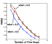
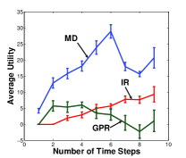
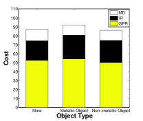
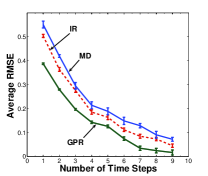
For our first group of experiments we analyze the performance of our technique w.r.t. the variables in our model, such as $w_{bel}$ and time, and, w.r.t. to sensor and object types. We observe that as more information gets sensed for the object, the RMSE value, shown in Figure 2(a), decreases over time. It takes on average $6-8$ time steps to predict the object type with $95\%$ or greater accuracy depending on the object type and the value of $w_{bel}$. We also observe that our model performs the best with $w_{bel}=0.5$ (in Equation 2), when the agent equally incorporates its private signal and also the market’s aggregated belief at each time step into its own belief update. Figure 2(b) shows the average utility of the agents based on their type. We can see that MD sensors get more utility because their costs of calculating and submitting reports are generally less, whereas GPR sensors get the least utility because they encounter the highest cost. This result is further verified in Figure 2(c) where we can see the costs based on sensor types and also based on object types. We observe that detecting a metallic object that is not a mine has the highest cost. We posit that it is because both MD and IR sensors can detect metallic content in the object and extra cost is due to the time and effort spent differentiating metallic object from a mine. Although most of the mines are metallic [10, 11], we can see that the cost of detecting a mine and a non-metallic object are similar because we require a prediction of at least $95\%$. Due to the sensitive nature of the landmine detection problem, it is important to ensure that even a non-metallic object is not a mine even if we encounter higher costs. However, despite MD’s high utility (Figure 2(b)) and low cost (Figure 2(c)), its error of classifying the object type is the largest, as can be seen from Figure 2(d).

In Table 2, we show how the decision maker’s decisions using our prediction market technique results in the deployment of different numbers and types of sensors over the time window of the object. We report the results for the value of belief update weight $w_{bel}=0.5$(used in Equation 2) while using our prediction market model, as well as using D-S and DDF. We see that non-metallic object classification requires less number of sensors as both MD and IR sensors can distinguish between metallic vs. non-metallic objects, and so, deploying just these two types of sensors can help to infer that the object is not a mine. In contrast, metallic objects require more time to get classified as not being a mine because more object features using all three sensor types need to be observed. We also observe that on average our aggregation technique using prediction market deploys a total of $6-8$ sensors and detects the object type with at least $95\%$ accuracy in $6-7$ time steps, while the next best compared DDF technique deploys a total of $7-9$ sensors and detects the object type with at least $95\%$ accuracy in $7-8$ time steps.

a	b	c

Figure 3: Comparison of our Prediction Market-based information aggregation with Dempster-Shafer and Distributed Data Fusion Techniques using different metrics: RMSE(a), NMSE(b), Information gain(c).

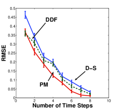
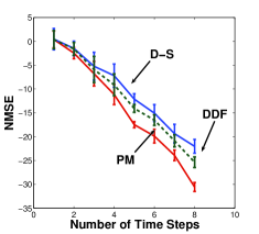
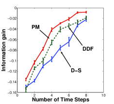
Our results shown in Figure 3(a) illustrate that the RMSE using our PM-based technique is below the RMSEs using D-S and DDF by an average of $8\%$ and $5\%$ respectively. Figure 2(b) shows that the NMSE values using our PM-based technique is $18\%$ and $23\%$ less on average than D-S and DDF techniques respectively. Finally, in Figure 2(c) we observe that the information gain for our PM-based technique is $12\%$ and $17\%$ more than D-S and DDF methods respectively.

6 Conclusions

In this paper, we have described a sensor information aggregation technique for object classification with a multi-agent prediction market and developed a payment function used by the market maker to incentivize truthful revelation by each agent. Currently, the rewards given by the market maker agent to the sensor agents are additional side payments incurred by the decision maker. In the future we plan to investigate a payment function that can achieve budget balance. We are also interested in integrating our decision making problem with the problem of scheduling robots(sensors), and, incorporating the costs to the overall system into the decision-making costs. Another direction we plan to investigate in the future is a problem of minimizing the time to detect an object in addition to the accuracy of detection. Lastly, we plan to incorporate our aggregation technique into the experiments with real robots.

References

- [1] Chen Y., Dimitrov S., Sami R., Reeves D.M., Pennock D.M., Hanson R.D., Fortnow L., Gonen R. Gaming Prediction Markets: Equilibrium Strategies with a Market Maker. Algorithmica J., 58(4):930–969, 2009.
- [2] Chen Y., Kash I. Information Elicitation for Decision Making. In AAMAS 2011, pages 175–182, 2011.
- [3] Cremer F., Schutte K., Schavemaker J.G.M, den Breejen E. A comparison of decision-level sensor-fusion methods for anti-personnel landmine detection. Information Fusion, 2(1):187–208, 2001.
- [4] Gneiting T. and Raftery A.E. Strictly proper scoring rules, prediction, and estimation. Journal of the American Stat. Assoc., 102(477):359–378, 2007.
- [5] Gros B., Bruschini C. Sensor technologies for the detection of antipersonnel mines: a survey of current research and system developments. In Proceedings of the International Symposium on Measurement and Control in Robotics, pages 509–518, 1996.
- [6] Hanson R. Logarithmic Market Scoring Rules for Modular Combinatorial Information Aggregation. Journal of Prediction Markets, 1(1):3–15, 2007.
- [7] Jumadinova J., Dasgupta P. A Multi-Agent System for Analyzing the Effect of Information on Prediction Markets. International Journal of Intelligent Systems, 26(1):383–409, 2011.
- [8] Makarenko A., Durrant-Whyte H. Decentralized Bayesian algorithms for active sensor networks. In Information Fusion 7, pages 418–433, 2006.
- [9] Manyika J., Durrant-Whyte H. Data fusion and sensor management. Prentice Hall, 1995.
- [10] Milisavljevi N., Bloch I. Sensor Fusion in Anti-Personnel Mine Detection Using a Two-Level Belief Function Model, Part C: Applications and Reviews. IEEE Transactions on Systems, Man, and Cybernetics, 33(2):269–283, 2003.
- [11] Milisavljevi N., Bloch I., Acheroy M. Characterization of Mine Detection Sensors in Terms of Belief Functions and their Fusion, First Results. In Proc. of the Third International Conference on Information Fusion, FUSION 2000, pages 15–22, 2000.
- [12] Mukherjee P., Sen S. Comparing Reputation Schemes for Detecting Malicious Nodes in Sensor Networks. The Computer Journal, 54(3):482–489, 2011.
- [13] Osborne M., Roberts S., Rogers A., Ramchurn S., Jennings N. Towards realt-time information processing of sensor network data using computationally efficient multi-output gaussian processes. In IPSN, pages 109–120, 2008.
- [14] Othman A., Sandholm T. Decision Rules and Decision Markets. In AAMAS 2010, pages 625–632, 2010.
- [15] Rosencrantz M., Gordon G., Thrun S. Decentralized sensor fusion with distributed particle filters. In IPSN, pages 55–62, 2003.
- [16] Vinyals M., Rodriguez-Aguilar J., Cerquides J. A Survey of Sensor Networks from a Multiagent Perspective. Computer Journal, 54(3):455–470, 2011.
- [17] Waltz E., Llinas J. Multisensor Datafusion. Artech House, 1990.
- [18] Wolfers J. and Zitzewitz E. Prediction Markets. Journal of Econ. Perspectives, 18(2):107–126, 2004.
- [19] Wu Q., Rao N., Barhen J., Iyengar S., Vaishnavi V., Qi H., Chakrabarty K. On Computing Mobile Agent Routes for Data Fusion in Distributed Sensor Networks. IEEE Trans. on Knowledge and Data Engineering, 16(6):740–753, 2004.