On the Spin-Down of Intermittent Pulsars

Abstract

Magnetospheres of pulsars are thought to be filled with plasma, and variations in plasma supply can affect both pulsar emission properties and spin-down rates. A number of recently discovered “intermittent” pulsars switch between two distinct states: an “on”, radio-loud state, and an “off”, radio-quiet state. Spin-down rates in the two states differ by a large factor, $\sim 1.5-2.5$, which is not easily understood in the context of current models. In this Letter we present self-consistent numerical solutions of “on” and “off” states of intermittent pulsar magnetospheres. We model the “on” state as a nearly ideal force-free magnetosphere with abundant magnetospheric plasma supply. The lack of radio emission in the “off” state is associated with plasma supply disruption that results in lower plasma density on the open field lines. We model the “off” state using nearly vacuum conditions on the open field lines and nearly ideal force-free conditions on the closed field lines, where plasma can remain trapped even in the absence of pair production. The toroidal advection of plasma in the closed zone in the “off” state causes spin-downs that are a factor of $\sim 2$ higher than vacuum values, and we naturally obtain a range of spin-down ratios between the “on” and “off” states, $\sim 1.2-2.9$, which corresponds to a likely range of pulsar inclination angles of $30{-}90^{\circ}$. We consider the implications of our model to a number of poorly understood but possibly related pulsar phenomena, including nulling, timing noise, and rotating radio transients.

1. Introduction

Pulsars spin down due to torques exerted by currents flowing on the surface of the neutron star. In the absence of magnetospheric plasma, the pulsar spins down due to magneto-dipole radiation (Michel, 1991; Beskin et al., 1993). Magnetospheric plasma allows for currents that can produce additional spin-down torques (Spitkovsky, 2006, hereafter S06), so variations in plasma supply can potentially modulate pulsar spin-down.

Several classes of pulsars have been identified that may exhibit such modulation. Nulling pulsars have radio emission that appears to shut off for a few to several tens of rotation periods. Since radio emission is presumably tied to the magnetospheric plasma, the nulling suggests that some process is affecting the plasma supply and/or currents above the polar caps (Wang et al., 2007; Zhang et al., 2007; Timokhin, 2010). Intermittent pulsars switch between an “on”, radio-loud, state in which they behave like normal radio pulsars, and an “off”, radio-quiet, state in which they produce no detectable radio emission for long periods of time. This process may be an extreme manifestation of nulling. The first two intermittent pulsars with published data have quite different duty cycles: PSR B1931+24 (Kramer et al., 2006, hereafter K06), with a period $P\approx 0.8$ s, cycled through the “on”–”off” sequence of states approximately once a month, whereas PSR J1832+0029 (Lyne, 2009), with a period $P\approx 0.5$ s, kept quiet for nearly two years between “on” cycles of unknown length. The spin-down rate for each of these pulsars is larger in the “on” state than in the “off” state by a factor $f_{{\rm on}\to{\rm off}}\simeq 1.5$. A third intermittent pulsar, PSR J1841-0500, was not detected for over $1.5$ years between “on” cycles, one of which appears to have lasted for at least a year (Camilo et al., 2011). This pulsar seems to have a spin-down ratio between “on” and “off” states of $f_{{\rm on}\to{\rm off}}\simeq 2.5$. Such substantial differences in spin-down rates suggest that the pulsar magnetosphere undergoes a dramatic reconfiguration as it transitions between the “on” and “off” states, yet such a transition was reported for PSR B1931+24 to take place in just over $10$ pulsar periods.

Intermittent pulsars offer a unique testbed of pulsar theory. K06 first proposed that in the “on” state plasma fills the pulsar magnetosphere and supports plasma processes that produce radio emission. The pulsar transitions to the “off” state when open field lines become depleted of charged radiating particles. K06 approximated the spin-down rate in the “off” state by the spin-down of a vacuum dipole and estimated the extra plasma currents needed to account for the observed spin-down of the “on” state. It is not clear, however, whether a working pulsar should naturally yield the required on-off spin-down ratio of this picture. The simplest model for the “on” state is the force-free magnetosphere, which has abundant charges everywhere. The force-free spin-down rate is larger than the vacuum spin-down rate by a factor $f_{{\rm ff}\to{\rm vac}}=(1+\sin^{2}\alpha)/(2/3\sin^{2}\alpha)$ (S06) that is greater than or equal to $3$ for all inclination angles $\alpha$. This is clearly incompatible with the observed values, $f_{{\rm on}\to{\rm off}}\simeq 1.5-2.5$ (Beskin & Nokhrina, 2007; Gurevich & Istomin, 2007). This suggests that, perhaps, we do not understand the spin-down power of the “off” state.

The shutoff of pair formation as the intermittent pulsar switches “off” allows plasma to escape along the open field lines, but the plasma in the closed zone is confined by the geometry of the field lines. This is an important physical effect that was not included in previous work (K06; Li et al. 2011, hereafter LST11;Kalapotharakos et al. 2011). The currents and charges associated with plasma trapped in the closed zone can increase the spin-down in the “off” state even if the open field lines are empty. Thus, in this paper, we model the “off” state using a simple two-zone prescription in which the closed zone is highly conducting and the open field lines are vacuum-like. We run resistive force-free simulations to directly solve for the magnetospheric geometry in the “on” and “off” states and test whether this model can produce the observed intermittent pulsar spin-down ratios. In Section 2 we describe the numerical code and setup. Section 3 illustrates our intermittent pulsar solutions and shows the spin-down results. Section 4 provides a brief summary of our results and their observational implications.

2. Setup

We employ a three-dimensional numerical code (see S06) that implements the finite difference time-domain scheme (FDTD, Taflove & Hagness, 2005) to evolve electromagnetic fields from Maxwell’s equations,

$$\partial_{t}\vec{E} =c\vec{\nabla}\times\vec{B}-4\pi\vec{j},$$

$$\partial_{t}\vec{B} =-c\vec{\nabla}\times\vec{E},$$ (1)

where the current $\vec{j}$ is given by

$$\vec{j}=\rho\vec{v}+\sigma\vec{E}_{\rm fluid}.$$ (2)

The fluid velocity $\vec{v}=c(\vec{E}\times\vec{B})/(B^{2}+E_{0}^{2})$ is the generalized drift velocity, $\vec{E}_{\rm fluid}=\gamma(\vec{E}+\vec{v}\times\vec{B})$ is the fluid frame electric field, $\gamma=(1-v^{2}/c^{2})^{-1/2}$, $E_{0}$ is the magnitude of $\vec{E}_{\rm fluid}$ (see LST11), $\rho$ is the charge density, and $\sigma$ is the plasma conductivity in the fluid frame. The central region of our grid is occupied by a conducting spherical star of radius $R_{*}$, rotating at angular velocity $\vec{\Omega}$, with embedded dipole field of magnetic moment $\vec{\mu}$ inclined relative to the rotation axis by angle $\alpha$. We resolve the light cylinder $R_{\rm LC}=c/\Omega$ with 80 cells and set $R_{*}=30$ cells. See LST11 for a detailed description of our code and resistive current formulation. We have verified that our solutions are converged with spatial resolution, as well as run sufficiently long so as to reach a steady state in the frame corotating with the pulsar.

In LST11 we showed that our resistive force-free formulation can capture both the vacuum and ideal force-free limits by varying the conductivity parameter. We model the “on” state as a magnetosphere with high conductivity $(\sigma/\Omega)^{2}=40$, our fiducial value representing force-free–like conditions for $R_{*}/R_{\rm LC}=3/8$. This is preferable to using an ideal force-free formulation as in S06, because our high conductivity solutions are numerically cleaner, especially in the current sheets (LST11). We model the “off” state as having conducting and vacuum-like regions separated sharply at the boundary of the closed field line region, which we approximate as the closed field lines of the force-free “on” state. Nonrotating dipole magnetic field lines are traced by the curves $s=s_{0}\sin^{2}\theta$ (Michel & Li, 1999), where $\theta$ is the angle from the magnetic axis, $s$ is spherical radius, and $s_{0}$, the maximum perpendicular distance of a field line from the magnetic axis, specifies which field line is under consideration. The closed field lines in the force-free solutions are typically stretched in the direction perpendicular to the magnetic axis as compared to vacuum dipole closed field lines. We use the surface $s=R_{\rm LC}\sin^{2}\theta(R_{\rm LC}\sin^{2}\theta/R_{*})^{k}$ to demarcate the closed field line region. The exponent $k$ is set at each inclination angle to best match the shape of the force-free closed zone (see Section 3 for illustrations of these demarcation surfaces), and the half-angle size of the conducting polar cap is given by $\theta_{\rm pc}=\sqrt{R_{*}/R_{\rm LC}}$. Interior to the demarcation surface, we set $(\sigma/\Omega)^{2}=40$, as in the “on” state. Exterior to the demarcation surface, we set $(\sigma/\Omega)^{2}=0.04$, a fiducial value representative of vacuum-like conditions for $R_{*}/R_{\rm LC}=3/8$. We pick this value over $\sigma/\Omega=0$ for better numerical accuracy when computing the field geometry. This choice of conductivity on open field lines and the exact shape of the demarcation surface have minimal effect on spin-down (see Section 3).

3. Results

Figure 1 shows magnetic field lines in the $\vec{\mu}-\vec{\Omega}$ plane for inclined dipoles at $\alpha=30^{\circ}$ (top), $60^{\circ}$ (middle), $90^{\circ}$ (bottom). Color is representative of the out-of-plane magnetic field (as in LST11). The left column shows the “off” state with abundant plasma in the closed zone but a shortage of plasma along open field lines. The red curves indicate the boundary between the conducting and vacuum-like regions in the illustrated cross-section of the magnetosphere. The right column shows the “on” state with abundant plasma everywhere. The magnetospheres in the “on” state are force-free–like, with conduction currents flowing along open field lines. The current returns through the current sheets and along the boundary of the closed field line region in the current layers. Gross features of the magnetosphere in the “off” state are vacuum-like, with large closed field line region and displacement currents contributing to spin-down. For reference we show a representative vacuum solution with inclination angle $\alpha=60^{\circ}$ in Figure 2. There are a number of important differences that distinguish the intermittent “off” state from the vacuum solutions. The current from toroidal advection of charged plasma in the closed zone leads to greater magnetic flux passing through the light cylinder and a larger fraction of open field lines. Further, poloidal conduction currents are present even outside the conducting closed zone. They are due primarily to the fluid advection term $\rho\vec{v}$ in the current and lead to greater magnetic field sweepback and stronger current sheets than in pure vacuum solutions.

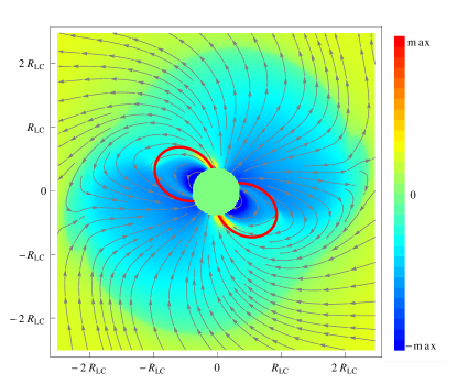
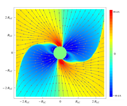
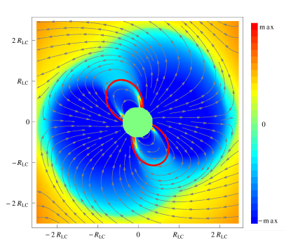
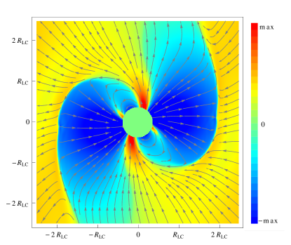
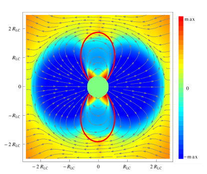
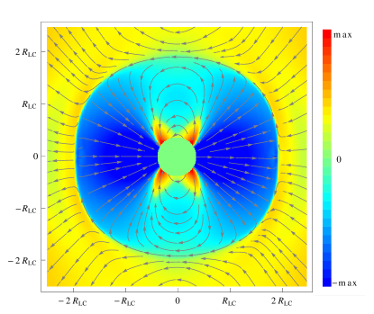
Figure 1.— Magnetic field lines in the $\vec{\mu}-\vec{\Omega}$ plane for inclined dipoles at $\alpha=30^{\circ}$ (top), $\alpha=60^{\circ}$ (middle), $\alpha=90^{\circ}$ (bottom). Color is representative of out-of-plane magnetic field into (red) and out of (blue) the page. The left column shows the “off” state with abundant plasma in the closed zone and vacuum-like conditions along open field lines. The red curves indicate the intersection with the $\vec{\mu}-\vec{\Omega}$ plane of the demarcation surface between these distinct conducting and vacuum-like regions. Gross features of the magnetosphere in the “off” state are vacuum-like, but the “off” states have more magnetic flux passing through the light cylinder and stronger magnetic field sweepback than vacuum solutions. The right column represents the “on” state with abundant plasma everywhere.

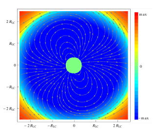
Figure 2.— Magnetic field lines in the $\vec{\mu}-\vec{\Omega}$ plane for a vacuum inclined dipole at $\alpha=60^{\circ}$. Color is representative of out-of-plane magnetic field into (red) and out of (blue) the page. There is large closed field line region, and displacement currents circulate and contribute to spin-down.

Figure 3 shows the spin-down luminosity, normalized by $L_{0}$ (where $L_{0}$ is $3/2$ times the power of the orthogonal vacuum rotator with finite $R_{*}/R_{\rm LC}=3/8$), as a function of inclination angle for both the “on” and “off” states of the magnetosphere. Spin-down luminosity is calculated as the surface integral of the Poynting flux over a sphere of radius $R_{\rm LC}$. We also show for reference the spin-down for the vacuum solution in the total absence of plasma. The “on” state spin-down is essentially the force-free spin-down. There is an uncertainty of roughly $10$% of $L_{0}$ in the force-free spin-down at low inclination angles due to stellar boundary effects and unphysical dissipation above the polar caps (see LST11). The spin-down in the “off” state lies between the force-free and vacuum spin-down values at all inclination angles. The spin-down of the aligned rotator in the “off” state is small, as the displacement currents are zero and large-scale conduction currents are weak. The open field lines carry minimal Poynting flux. Inclined dipole open field lines carry Poynting flux, however, and the larger magnetic flux passing through the light cylinder in the “off” state results in higher spin-down than in the vacuum solution. This increase in Poynting flux over vacuum spin-down in the “off” state is largest at high inclination angles, where the open field lines in the vacuum solutions carry the most Poynting flux. The advective poloidal conduction currents also lead to higher spin-down since they cause larger magnetic field sweepback than in vacuum solutions. We evaluated the relative contributions of these two effects to higher spin-down over vacuum solutions by killing the advection current term $\rho\vec{v}$ outside the closed zone. The larger magnetic flux passing through the light cylinder is responsible for upwards of two-thirds of the increase in Poynting flux over vacuum spin-down in the “off” state.

Figure 3.— Spin-down luminosity dependence on inclination angle for the force-free–like “on” state, the “off” state, and the vacuum solution. The “off” state spin-down naturally lies between the force-free and vacuum spin-down values for all inclination angles. spin-down is normalized by $3/2$ times the spin-down power of the orthogonal vacuum rotator.

The spin-down in the simulated “off” state is relatively insensitive to the size of the conducting closed zone. We varied the volume of the conducting closed zone by a factor of a few while keeping the size of the polar cap fixed, and we find that spin-down changes by less than $20$% of $L_{0}$ at all inclination angles. It is not the total size of the conducting closed zone, but rather its extent on the stellar surface that is more important in determining the gross magnetospheric properties. Blocking radial currents near the stellar surface limits the large-scale poloidal current circuit. Spin-down also depends very weakly on the fiducial values of $\sigma/\Omega$ that we pick to represent highly conducting and vacuum conditions. We checked this by setting the conductivity to $\sigma/\Omega=0$ instead of $(\sigma/\Omega)^{2}=0.04$ along open field lines, and we find that the resulting spin-down is offset by less than $20$% of $L_{0}$ for all inclination angles. The aligned “off” state spin-down drops to zero in this case, as we expect, since the large-scale conduction currents have been eliminated. We also tried setting the closed zone to have conductivity $(\sigma/\Omega)^{2}=20$ instead of $(\sigma/\Omega)^{2}=40$, and spin-down results change by less than $10$% of $L_{0}$ at all inclination angles.

The most relevant observational parameter in the context of intermittent pulsars is the ratio of spin-down power in the “on” and “off” states, $f_{{\rm on}\to{\rm off}}$. Figure 4 shows this ratio for our models. We emphasize that these models provide a physically well-motivated set of solutions to describe both the “on” and “off” states of intermittent pulsars. Assuming a uniform distribution of pulsar inclination angles, we expect two-thirds of intermittent pulsars to have $f_{{\rm on}\to{\rm off}}$ between $1.2-2.9$. Known intermittent pulsars fall within this range (K06, Lyne, 2009; Camilo et al., 2011). Uncertainties in the exact charge configuration and charge transport properties in the “off” state magnetosphere imply error bars associated with our calculation of the ratio $f_{{\rm on}\to{\rm off}}$. The uncertainty is of order $10$% at inclination angle $\alpha=90^{\circ}$ and rises with decreasing inclination angle to a factor of order $2$ at $\alpha=30^{\circ}$. Below $\alpha=30^{\circ}$ the ratio $f_{{\rm on}\to{\rm off}}$ rises above 3 due to the small spin-down of the aligned rotator in the “off” state, but there are large uncertainties in the exact value of $f_{{\rm on}\to{\rm off}}$ in this regime.

Figure 4.— The ratio of spin-down power between the “on” and “off” states, $f_{{\rm on}\to{\rm off}}$, as a function of inclination angle. We obtain $f_{{\rm on}\to{\rm off}}\sim 1.2-2.9$ for $\alpha>30^{\circ}$. Known intermittent pulsars have $f_{{\rm on}\to{\rm off}}$ in this range.

A major improvement of our intermittent pulsar models over existing work (LST11) lies in the treatment of accelerating potential drops, which can be used as a fiducial measure of energy gain as particles fly away from the stellar surface. We define the potential drops as in LST11, i.e., as the line integral along magnetic field lines of the corotating electric field $\vec{E}^{\prime}=\vec{E}+(\vec{\Omega}\times\vec{r})\times\vec{B}/c$. In ideal force-free solutions the potential drops vanish, as $\vec{E}\cdot\vec{B}=0$, but they increase monotonically with increasing bulk resistivity. Previously, we implemented a constant conductivity $\sigma/\Omega$ throughout the magnetosphere. As the polar cap played no fundamental role in these models, open field line potential drops were generally limited by the full pole-to-equator potential drop, yielding unphysically large potential drops of order $10^{16}$ V. Our new models for the “off” state introduce conducting plasma in the closed field line zone, effectively shielding the potential drop there. The potential drops are then limited by the polar cap potential drop $V_{\rm pc}=|\vec{\mu}|/R_{\rm LC}^{2}$. For typical pulsars with periods $P\sim 1$s, we obtain characteristic potential drop of $\sim 10^{12}$ V, more in line with expectations.

4. Discussion

We have developed an improved numerical method for solving pulsar magnetospheres with resistivity, and we apply it to describe intermittent pulsars in a self-consistent manner. In the “on” state, plasma is abundant everywhere, and the instabilities in this plasma generate coherent radio emission. In the “off” state plasma has leaked off the open field lines, suppressing the open field line currents. The radio emission is hence shut off. Plasma remains trapped in the closed zone, however, and the current from toroidal advection of these charges leads to spin-down values that are a factor of $\sim 2$ larger than vacuum values. This allows us to naturally produce spin-down ratios $f_{{\rm on}\to{\rm off}}\sim 1.2-2.9$ for inclination angle in the range $\alpha=30^{\circ}-90^{\circ}$, consistent with observations, and we obtain realistic values for accelerating potential drops, $V_{\rm drop}\sim 10^{12}$ G. In our model the spin-down ratio $f_{{\rm on}\to{\rm off}}$ takes on its minimum value at $\alpha=90^{\circ}$ and increases monotonically with decreasing inclination angle. Hence, given an observed spin-down ratio $f_{{\rm on}\to{\rm off}}$ for an intermittent pulsar, we can predict, within errors, the pulsar’s inclination angle. Alternatively, given the pulsar inclination angle from, e.g., polarization vector sweep data, we can predict the spin-down ratio $f_{{\rm on}\to{\rm off}}$ if the pulsar displays clear “on” and “off” states. A verification of our predictions would lend strong support to the idea that abrupt changes in plasma supply on open field lines can play an important role in determining the emission properties and spin-down rates of real pulsars.

One potential limitation of our models relates to the spatial distribution of conductivity in the magnetosphere. We specify only a conducting torus located in the plane perpendicular to the magnetic axis. In fact, rotation of a conducting neutron star leads to unipolar induction, and domes of negative charge form above the magnetic poles even in the absence of a pair cascade if the work function of the surface is low (Krause-Polstorff & Michel, 1984, 1985; Petri et al., 2002a, b; Spitkovsky & Arons, 2002; Spitkovsky, 2004). We explored this effect by prescribing additional conducting domes above the magnetic poles, setting $(\sigma/\Omega)^{2}=40$ interior to the surfaces specified by $s=R_{\rm LC}\cos^{2}\theta$. Spin-down values increase at all inclination angles by an offset of less than $20$% of $L_{0}$, but the spin-down ratio $f_{{\rm on}\to{\rm off}}$ remains within the errors quoted in Section 3.

It is important to note that at present the precise mechanism by which the plasma supply is turned on and off is still unclear. In at least one intermittent pulsar case the switching between different spin-down rates is quasi-periodic (K06), implying that the processes supplying and limiting plasma alternately recur. Intermittency may actually be the same basic process as nulling, the crucial difference being that the “off” state lasts months to years instead of from a few rotation periods up to days. In this light, timing noise can in some instances be caused by nulling events that are not resolved by the observations. The pulsar timing data in the Jodrell Bank data archive are typically smoothed and do not resolve features that occur on time scales shorter than a few tens of days (see Hobbs et al., 2010; Lyne et al., 2010). Suppose recurring nulling events last for an accumulated time that is of order a few percent of the time that the pulsar behaves normally. Since in our model the spin-down in the “off” state is typically of order $1/2$ that in the “on” state, the resulting spin-down luminosity in a state with unresolved nullings could easily be modified by $\sim 1$%. Lyne et al. (2010) established a connection between timing noise and mode changing, when the pulse profile of the pulsar changes to a different shape, but they do not see mode changing in all pulsars that exhibit timing noise. It is possible that some of these pulsars undergo nulling events, which leads to variation in spin-down rate and the observed timing noise. The mode changing is presumably due to changes in the magnetospheric configuration. One possibility is that it is an intermediate state between our “on” and “off” states in which some but not all of the plasma along open field lines has leaked away. These intermediate states could lead to a number of observed pulsar features including jitter, subpulse drift, precursors, and interpulses, though such ideas are at present still speculative. Another possible cause for changing pulse profiles is the presence of multiple components to the emission, e.g., the core and conal components, and one or more components being modified or shut off by changes in plasma supply.

If the “on” and “off” states of the pulsar can last anywhere from a few periods to years, it is further conceivable that Rotating Radio Transients (RRATs) are another manifestation of the process captured by our model. RRATs are rotating neutron stars that occasionally emit pulses, usually isolated, but in a few instances in a string of several (McLaughlin et al., 2006; Palliyaguru et al., 2011). It has not been ruled out that RRATs are an extreme form of nulling, and we envision RRATs as pulsars that spend the majority of their time in our “off” state, but turn “on” from time to time and emit pulses. If future observations are able to establish a more definitive link between the seemingly disparate processes of intermittency, nulling, timing noise, and RRATs, it would be an important step in our understanding of pulsar physics.

AT acknowledges support by the Princeton Center for Theoretical Science fellowship. AS is supported by NSF grant AST-0807381 and NASA grants NNX09AT95G and NNX10A039G. The simulations presented in this article were performed on computational resources supported by the PICSciE-OIT High Performance Computing Center and Visualization Laboratory.

References

- Beskin et al. (1993) Beskin, V. S., Gurevich A. V., Istomin, Ya. N. 1993, Physics of the Pulsar Magnetosphere (Cambridge: Cambridge University Press)
- Beskin & Nokhrina (2007) Beskin, V. S. & Nokhrina, E. E. 2007, Ap&SS, 308, 569
- Camilo et al. (2011) Camilo, F., Ransom, S. M., Chatterjee, S., Johnston, S., & Demorest, P. 2011, arXiv:1111.5870
- Gurevich & Istomin (2007) Gurevich, A. V., & Istomin, Y. N. 2007, MNRAS, 377, 1663
- Hobbs et al. (2010) Hobbs, G., Lyne, A. G., & Kramer, M. 2010, MNRAS, 402, 1027
- Kalapotharakos et al. (2011) Kalapotharakos, C., Kazanas, D., Harding, A., & Contopoulos, I. 2011, arXiv:1108.2138
- Kramer et al. (2006) Kramer, M., Lyne, A.G., O’Brien, J.T., Jordan, C.A., Lorimer, D.R. 2006, Sci, 312, 549
- Krause-Polstorff & Michel (1984) Krause-Polstorff, J., & Michel, F. C. 1984, MNRAS, 213, 43
- Krause-Polstorff & Michel (1985) Krause-Polstorff, J., & Michel, F. C. 1985, A&A, 144,72
- Li et al. (2011) Li, J., Spitkovsky, A., & Tchekhovskoy, A. 2011, arXiv:1107.0979
- Lyne (2009) Lyne, A. G. 2009, ASSL, 357, 67
- Lyne et al. (2010) Lyne, A., Hobbs, G., Kramer, M., Stairs, I., & Stappers, B. 2010, Science, 329, 408
- McLaughlin et al. (2006) McLaughlin, M. A., Lyne, A. G., Lorimer, D. R., et al. Nature, 439, 817
- Michel (1991) Michel, F. 1991, Theory of Neutron Star Magnetosphere (Chicago: University of Chicago Press)
- Michel & Li (1999) Michel, F. C. & Li, H. 1999, Physics Reports, 318, 227
- Palliyaguru et al. (2011) Palliyaguru, N. T., McLaughlin, M. A., Keane, E. F., et al. 2011, MNRAS, 1871
- Petri et al. (2002a) Petri, J., Heyvaerts, J., & Bonazzola, S. 2002a, A&A, 384, 414
- Petri et al. (2002b) Petri, J., Heyvaerts, J., & Bonazzola, S. 2002b, A&A, 387, 520
- Spitkovsky (2004) Spitkovsky, A. 2004, IAUS, 218, 357
- Spitkovsky (2006) Spitkovsky, A. 2006, ApJ, 648, L51
- Spitkovsky & Arons (2002) Spitkovsky, A., Arons, J. 2002, in ’Neutron Stars in Supernova Remnants’, eds P. O. Slane and B. M. Gaensler, (San Francisco: ASP), 271, 81
- Taflove & Hagness (2005) Taflove, A. N. & Hagness, S. C. 2005, Computational Electrodynamics: The Finite-Difference Time-Domain Method, Third Edition (Norwood, MA: Artech House)
- Timokhin (2010) Timokhin, A. N. 2010, MNRAS, 408, 41
- Wang et al. (2007) Wang, N., Manchester, R. N., & Johnston, S. 2007, MNRAS, 377, 1383
- Zhang et al. (2007) Zhang, B., Gil, J., & Dyks, J. 2007, MNRAS, 374, 1103