Clustering of Sloan Digital Sky Survey III Photometric Luminous Galaxies: The Measurement, Systematics and Cosmological Implications
Abstract
The Sloan Digital Sky Survey (SDSS) surveyed 14,555 square degrees, and delivered over a trillion pixels of imaging data. We present a study of galaxy clustering using 900,000 luminous galaxies with photometric redshifts, spanning between and , constructed from the SDSS using methods described in Ross et al. (2011). This data-set spans 11,000 square degrees and probes a volume of , making it the largest volume ever used for galaxy clustering measurements. We describe in detail the construction of the survey window function and various systematics affecting our measurement. With such a large volume, high precision cosmological constraints can be obtained given a careful control and understanding of the observational systematics. We present a novel treatment of the observational systematics and its applications to the clustering signals from the data set. In this paper, we measure the angular clustering using an optimal quadratic estimator at 4 redshift slices with an accuracy of with bin size of on scales of the Baryon Acoustic Oscillations (BAO) (at ). We also apply corrections to the power-spectra due to systematics, and derive cosmological constraints using the full-shape of the power-spectra. For a flat CDM model, when combined with Cosmic Microwave Background Wilkinson Microwave Anisotropy Probe 7 (WMAP7) and constraints from using 600 Cepheids observed by Wide Feild Camera 3 (WFC3) (HST) , we find and to be . For an open CDM model, when combined with WMAP7 + HST, we find , improved over WMAP7+HST alone by . For a wCDM model, when combined with WMAP7+HST+SN, we find , and to be , which is competitive with the latest large scale structure constraints from large spectroscopic surveys such as SDSS Data Release 7 (DR7) (Reid et al. 2010, Percival et al. 2010, Montesano et al. 2011) and WiggleZ (Blake et al. 2011). We also find that systematic-corrected power-spectra gives consistent constraints on cosmological models when compared with pre-systematic correction power-spectra in the angular scales of interest. The SDSS-III Data Release 8 (SDSS-III DR8) Angular Clustering Data allows a wide range of investigations into the cosmological model, cosmic expansion (via BAO), Gaussianity of initial conditions and neutrino masses. Here, we refer to our companion papers (Seo et al. 2011, de Putter et al. 2011) for further investigations using the clustering data. Our calculation of survey selection function, systematics maps, likelihood function for COSMOMC package will be released at http://portal.nersc.gov/project/boss/galaxy/photoz/.
1. Introduction
The distribution of light in the Universe has long been used as a probe into the structure of the Universe. Einstein wrote of the distribution of stars as possibly being uniform on average over large enough distances in 1917 when he discussed the structure of the Universe. Hubble tested the uniformity of distribution of faint nebulae in 1926. As the structure of the Universe unfolds, distribution of light from objects such as galaxies has remained a powerful cosmological probe (Peebles, 1973; Groth, 1973; Wang et al., 1999; Hu, 1999; Eisenstein et al., 1999).
Smoothed over large scales, we expect galaxy density to have a simple relationship to the underlying matter density; this implies that the clustering of galaxies at large scales is directly related to the clustering of the underlying matter and is thus a sensitive probe of both the initial conditions of the Universe and its subsequent evolution. It is therefore not surprising that a large fraction of the effort in observational cosmology had been devoted to measuring the spatial distribution of galaxies, as in the CfA Redshift Survey (Huchra et al., 1983),The APM Galaxy Survey (APM, Maddox et al., 1990), The DEEP survey111http://deep.berkeley.edu/ (DEEP, Koo, 1998), VIMOS-VLT Deep Survey (VVDS, Le Fèvre et al., 2005), Two-Degree Field Galaxy Redshift Survey (2dFGRS, Cole et al., 2005),The Two Micron All sky Survey (2MASS, Skrutskie et al., 2006), COSMOS (Scoville et al., 2007), Canada-France-Hawaii Telescope Legacy Survey222http://www.cfht.hawaii.edu/Science/ (CFHTLS, Ilbert et al., 2006), Galaxy And Mass Assembly survey (GAMA, Driver et al., 2009), The WiggleZ Survey (Blake et al., 2010), the Sloan Digital Sky Survey (SDSS, York et al., 2000). By 2008, the SDSS333www.sdss.org has probed with galaxies, while the current SDSS-III(Eisenstein et al., 2011) will finish surveying in 2014. The planned Large Synoptic Survey Telescope (LSST)444http://www.lsst.org will observe of the Universe.
Hidden in the ever-increasing volume of surveyed Universe, is the wealth of cosmological information that had not been fully exploited. In particular, the large scale clustering of any mass tracer, usually characterized by its power-spectrum, in the Universe contains three features that are of significant interest to contemporary cosmologists. The first distinguishing feature is oscillations in the power-spectrum caused by acoustic waves in the baryon-photon plasma before hydrogen recombination at , called Baryon Acoustic Oscillations (hereafter BAO) (Peebles & Yu, 1970; Sunyaev & Zeldovich, 1970; Bond & Efstathiou, 1984; Holtzman, 1989; Hu & White, 1996; Eisenstein & Hu, 1998). The BAO technique has emerged as the new precision cosmology probe, especially in discerning the properties of this unknown dark component of the Universe "Dark Energy". The BAO was first observed in early 2005 both in the SDSS Luminous Red Galaxy sample (Eisenstein et al., 2005), the 2dFGRS data (Cole et al., 2005) and in 2006 by using photometric Luminous Galaxies (LRGs) in of SDSS (Padmanabhan et al., 2007). However, neither of the signals were strong enough to place strong cosmological constraints via BAO. Second, the largest scales of the power-spectrum can be used to constrain the primordial potential of the Universe, thus testing inflation. In particular, Dalal et al. (2008) has pointed out the relationship between non-gaussianity of the potential in the early Universe (due to various possible inflationary scenarios) and the large scale power of mass tracer in the Universe. Finally, at , the power spectrum turns over from a slope (for a scale invariant spectrum of initial fluctuations), to a spectrum, caused by modes that entered the horizon during radiation-dominated era and were therefore suppressed. The precise position of this turnover is thus determined by the size of the horizon at matter-radiation equality. It corresponds to a physical scale determined by the total matter densities and radiation densities . In particular, with a large survey such as SDSS, various groups had used the large scale power-spectrum to put stringent constraints on cosmological parameters, most notably Zehavi et al. (2002); Tegmark et al. (2004); Eisenstein et al. (2005); Padmanabhan et al. (2007); Percival et al. (2010); Reid et al. (2010).
The SDSS has now surveyed , and with appropriate photometric selection, we can construct a large uniform sample of the photometric luminous red galaxies (Ross et al., 2011), and their photometric redshifts that can be easily calibrated using the acquired spectroscopic redshifts of a uniform sub-sample () of the photometric galaxies. This approach allows the possibility of using both standard rulers (from the turn over scale of power spectrum, and also the baryon acoustic oscillations) to acquire cosmological constraints.
We make use of this opportunity to derive one of the most accurate measurements of the galaxy angular power-spectra achieved to date. We start with the five band imaging of the SDSS-III DR8; Aihara et al. (2011); Eisenstein et al. (2011)), and photometrically select a sample of luminous red galaxies, following the CMASS galaxy selection detailed in White et al. (2011); the details of the construction of the sample and the redshift distribution is described in Ross et al. (2011). We then measure the angular clustering power spectra as a function of redshift with an optimal quadratic estimator, which is proved to provide the best statistical error-bar when the field is Gaussian. The galaxy density field is not Gaussian on small scales, due to non-linear evolution; however, at relatively large scales, which are the scales we are concerned here, the field is close to Gaussian. We will discuss this issue in detail in the paper. With such a large volume of data, we realize that the effects of large scale systematics are not negligible. To gauge and correct the effects of large scale systematics, we develop a novel method in correcting the large scale systematics given that we know the list of possible systematics. We construct the maps of various systematics, and calculate their cross-correlation with the galaxy density, the systematic auto-correlations and cross-correlations. We can then correct for these systematics applying this new method.
The paper is organized as follows : Sec. 2 describes the construction of the sample; Sec. 3 then presents the theory and measurement of the angular power spectra; Sec. 4 discusses the various potential systematics and the novel method applied in correcting for the observational systematics. Sec. 6.1 describes the validation of the cosmological parameter fitting method, and Sec. 7 summarizes the cosmological constraints themselves. We conclude in Sec. 8.
Wherever not explicitly mentioned, we assume best fit WMAP7 (Larson et al., 2011) parameters (from model lcdm+sz+lens as specified on LAMBDA website 555http://lambda.gsfc.nasa.gov/product/map/dr4/parameters.cfm), which are: a flat CDM cosmology with , , , and .
2. The Data
2.1. Observations
The Sloan Digital Sky Survey (SDSS; York et al. (2000); Eisenstein et al. (2011)) mapped over a quarter of the sky using the dedicated Sloan Foundation 2.5 m telescope located at Apache Point Observatory in New Mexico (Gunn et al., 2006). A drift-scanning mosaic CCD camera (Gunn et al., 1998; Gunn et al., 2006) imaged the sky in five photometric band-passes (Fukugita et al., 1996; Smith et al., 2002) to a limiting magnitude of r. The imaging data were processed through a series of pipelines that perform astrometric calibration (Pier et al., 2003), photometric reduction (Lupton et al., 2001) and photometric calibration (Padmanabhan et al., 2008). In particular, Baryon Oscillations Spectroscopic Survey (hereafter BOSS) which is a part of SDSS III (Eisenstein et al., 2011; Aihara et al., 2011), has completed an additional 3000 square degrees of imaging and is now obtaining spectra of a selected subset of 1.5 million galaxies. The targets are assigned to spectroscopic plates (tiles) using an adaptive tiling algorithm based on Blanton et al. (2003), and observed with a pair of fiber-fed spectrographs.
The availability of large uniform photometric data-set prompted the start of this project, thus a series of papers, starting with the generation of the photometric redshifts catalog by Ross et al. (2011), which uses 112,778 of BOSS spectra as a training sample for photometric catalog. The photometric redshift catalog contains over 1.6 million objects, and 900,000 of these objects lie within our imaging mask and the selected redshift range ( < z < ). The redshift range is selected so that it is nearly completely independent from DR7 analysis of LRG clustering using spectroscopy which stops at (Reid et al., 2010; Percival et al., 2010); this allows for possibility of trivial combination of likelihoods. These galaxies are among the most luminous galaxies in the universe and trace a large cosmological volume while having high enough number density to ensure shot-noise is not a dominant contributor to the clustering variance. The majority of the galaxies have spectral energy distributions ( , see Masters et al. (2011) and private communication with the BOSS galaxy-evolution group) that are distinctive of old stellar populations.
2.2. Defining Luminous Red Galaxies
We make use of the CMASS sample from BOSS, which is defined in White et al. (2011) and Ross et al. (2011); and we write down the criteria here again for convenience:
| (1) |
where
| (2) |
The magnitudes denoted by ”cmod” are ”cmodel magnitudes” (see White et al. (2011) for more discussions), and the colors are defined with model magnitudes, except for , which is the magnitude in the spectroscopic fiber (Stoughton et al., 2002; Abazajian et al., 2004). Note that we applied , although the current BOSS target selection has moved the limit from to . All magnitudes are extinction corrected using maps of Schlegel et al. (1998).
In addition to constructing galaxy density maps, we created several additional maps that we use to reject regions heavily affected by sample systematics such as poor sky or stellar density, and to make sure our final power-spectra are free of systematics. These include (i) a map of the full width at half-maximum (FWHM) of the point-spread function (PSF) in band; (ii) a map of stellar density ( stars); (iii) a map of sky brightness in -band in nanomaggies666http://data.sdss3.org/datamodel/glossary.html#nanomaggies/; (iv) 3 map of the color offsets in , and from Schlafly et al. (2010); (v) a map of Galactic extinction simply rescaled from the extinction maps from Schlegel et al. (1998).
2.3. Angular and Redshift Distributions
To interpret the clustering of any sample, one must characterize the expected distribution of the sample as if it is completely random. This involves understanding both the angular and radial selection function in addition to the expected galaxy density, which is characterized by its mean density.
To characterize the angular window function, we generate the complete angular mask of the survey following the procedures described below. The observed sky is defined as a union of all fields. Determining the window function requires identifying the fields that cover each position on the sky and deciding which of those fields should be considered primary at that position. There is a unique set of disjoint polygons on the sky defined by all the field boundaries, which are calculated using MANGLE package 777http://spae.mit.edu/m̃olly/mangle(Hamilton, 1993; Hamilton & Tegmark, 2004; Swanson et al., 2008) and each field can be divided into multiple polygons. We now must decide which fields are primary for each polygon in the sky; the process is described in Aihara et al. (2011) in detail. Once we determine which fields are primary for all the polygon in the sky, we make a cut on the field observing conditions (SCORE 0.6; for more details on SCORE, see Aihara et al. (2011) or the SDSS-III webpage 888sdss3.org). We now have an unified MANGLE polygon file that includes all the fields that are imaged in the entire SDSS footprint, with the correctly assigned primary fields with good observing conditions. We call this the "full imaging mask", as plotted in Figure 1. The color in Figure 1 represents the date at which the imaging data was taken. The striped pattern perpendicular to the scanning direction is easily visible, and we can also see that the north and south Galactic caps are observed at significantly different epoch of the survey. This provides hint as to what potential observational systematic effects would look like. To create a more restrictive mask which is catered towards photometric red galaxies, we proceed to exclude regions where (Scranton et al., 2002; Ross et al., 2006; Padmanabhan et al., 2007; Ho et al., 2008), which is almost identital to , when seeing in the -band exceeds in FWHM, and masking regions around stars in the Tycho astrometric catalog (Høg et al., 2000). The final angular selection function covers a solid angle of square degrees, and is shown in Fig. 2.
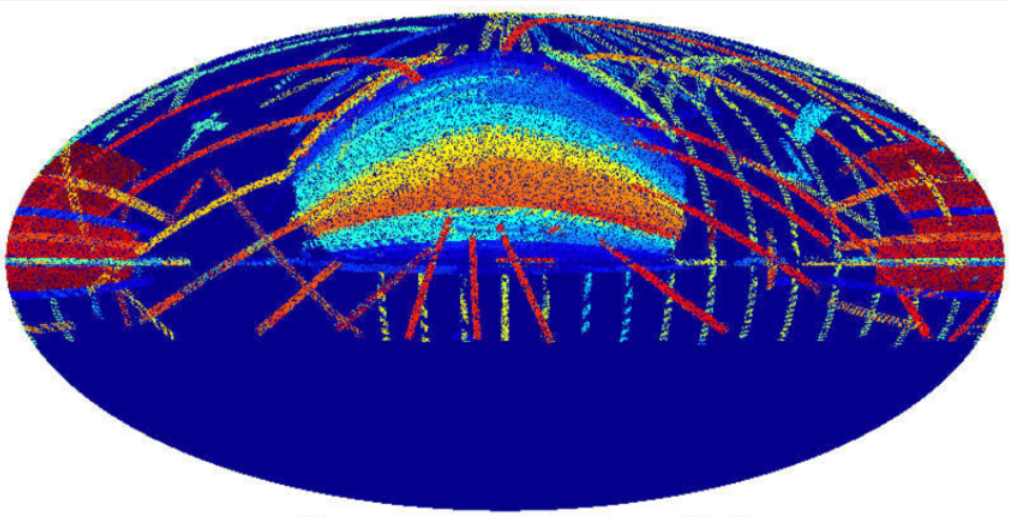
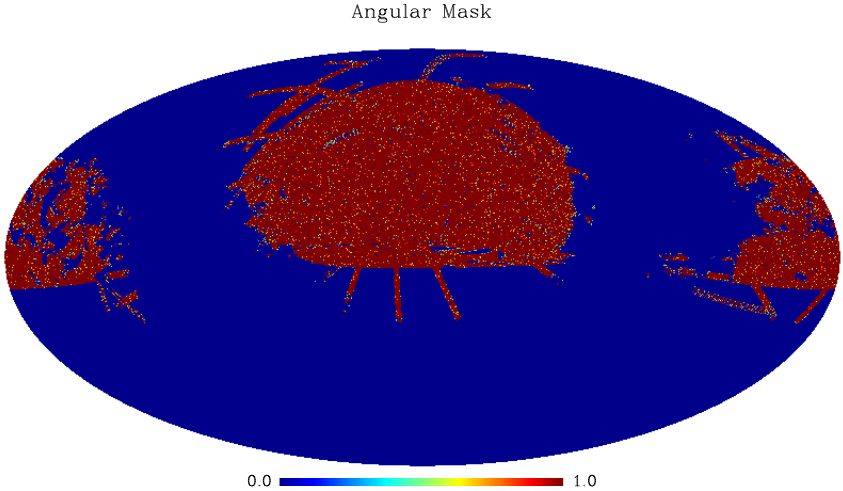
Applying the selection criteria in Sec 2.2 to the 14,555 of photometric SDSS imaging considered in this paper yields a catalog of approximately 1,500,000 galaxies. Applying the angular selection function as shown in Fig. 2 to the Ross et al. (2011) photometric redshift catalog yields a sample of 872,921 objects, 96% of which are believed to be galaxies (3% are stars, and 1% are quasars, according to statistics gathered in the spectroscopic sub-sample; Ross et al. (2011)). For every object, photometric redshifts and probabilities of being a galaxies were determined using the ANNz Neural Network (Collister & Lahav, 2004; Firth et al., 2003). The calibration and accuracy of these data are discussed in detail in Ross et al. (2011). In the range considered in this paper,the redshifts have calibrated errors at and at . We pixelize these galaxies as a weighted (with the probabilities of being a galaxy) number overdensity, , onto a HEALPix pixelization (Gorski et al., 1999) of the sphere, with 12,582,912 pixels over the whole sphere (HEALPix resolution 10, nside=1024), each pixel covers a solid angle of 11.8 . These pixelized maps are used directly to compute the angular power-spectra using optimal quadratic estimator. The optimal quadratic estimator does not down-sample input pixelized maps, rather, it computes the covariance matrix directly from these pixelized maps, and this will be discussed further in 3.4.
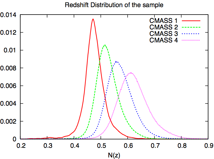
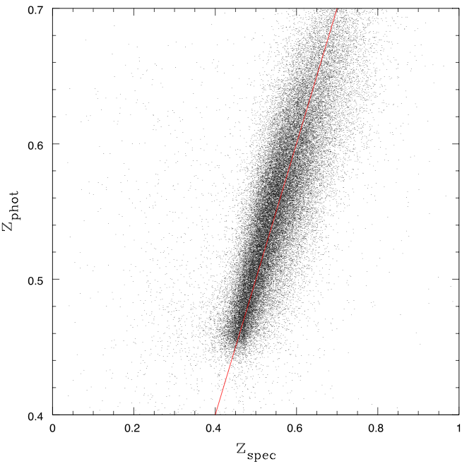
The sample is divided into 6 photometric redshift slices of thickness starting at for CMASS sample (CMASS 0 through CMASS 5, see Table 2.3 for details), and the underlying redshift distributions for each slice are calculated using BOSS spectroscopic redshift of the same sample. The redshift distribution of the sample is plotted in Fig. 3. We can see that although the majority of the objects in one photometric-redshift bin is in their corresponding true redshift bin, a significant fraction of them fall into neighboring bins. The comparisons of these photometric redshifts to the spectroscopic redshifts (obtained via SDSS III spectra) are plotted in Fig. 4, while properties of the different slices are summarized in Table 2.3. We see that the numbers of galaxies in both the first and the last bins are significantly smaller than the others, therefore, we decide to drop these 2 bins from our analysis. This decision is also facilitated by the fact that we wish to have a nearly independent sample from the Reid et al. (2010); Percival et al. (2010) LRG clustering analysis, thus allowing for simple combination of their likelihoods in the cosmological parameter analysis.
| Label | |||
|---|---|---|---|
| CMASS 0 | 0.425 | 23517 | |
| CMASS 1 | 0.475 | 154531 | 1.92 0.06 |
| CMASS 2 | 0.525 | 198132 | 1.98 0.05 |
| CMASS 3 | 0.575 | 190603 | 2.19 0.05 |
| CMASS 4 | 0.625 | 121181 | 2.19 0.05 |
| CMASS 5 | 0.675 | 54744 |
2.4. Sample Systematics
There are a number of potential systematic effects in photometric samples that contaminate clustering: stellar contamination and obsuration, seeing variations, sky brightness variations, extinction and color offsets (such as those described in Schlafly et al. (2010)). Ross et al. (2011) had extensive discussions on these potential systematics; we will concentrate on the particular effects from various systematics on the angular power-spectra in the range of scales that affects our science analysis.
The above cuts remove only parts of the sky that are significantly affected by extinction and seeing variations. With such a large sky coverage, an accurate determination of the angular power-spectra of the the large scale tracer is only possible through an thorough understanding of the systematics. However, if we only retain parts of the sky that have the minimum systematics effects; we must remove most of the coverage, as we have demonstrated in Ross et al. (2011). Therefore, we developed a novel way of dealing with residual sample systematics which we will discuss in Sec. 5 in detail.
3. The Angular Power Spectrum
As was noted in the introduction, the angular power-spectrum contains information of both the growth and the expansion of the Universe through two standard rulers of the Universe: the baryon acoustic oscillations and the matter-radiation equality turn-over scale; thus the shape of the power-spectrum. In this section, we will describe both the theory and the computation of angular power spectrum.
3.1. From galaxy distributions to angular power-spectrum
The intrinsic angular galaxy fluctuations are given by:
| (3) |
where is an assumed scale-independent bias factor relating the galaxy overdensity to the mass overdensity, i.e. , is the normalized selection function, and is the comoving distance to redshift . We focus on the auto power-spectrum of the galaxies:
| (4) |
where is the matter power spectrum today as a function of the wave number , and the function is
| (5) |
The Limber approximation, which is quite accurate when is not too small (), can be obtained from Eq. (4) by setting and using the asymptotic formula that (when ). We find that the substitution is a better approximation to the exact expressions than . Note that is the order spherical Bessel function. On large scales where the mass fluctuation , the perturbations grow according to linear theory = .
For auto-correlation, applying Limber approximation will change Eq. 4 to the following:
| (6) |
For cross-correlation between two different large scale structure samples (be it different selection functions, redshift distributions, different biases), we can write the cross-correlation as follows:
| (7) |
where can have different biases, redshift dependence etc.
We have not yet distinguished between the galaxy and the matter angular power-spectrum yet. Throughout this paper, we simply assume
| (8) |
where and are the galaxy and matter angular power spectra; is the linear galaxy bias, is a constant shot noise term which is estimated by the optimal quadratic estimator and is a constant term that is fitted as a freely floating parameter. This is a good approximation on large scales, but breaks down on smaller scales; we defer a discussion of its regime of validity, as well as the nonlinear evolution of the power spectrum to a later section of this paper 3.3.
Throughout the paper, we adopt this linear redshift independent (within our redshift slice) bias model with a constant shot noise term. The bias and the shot noise term of galaxy sample for the various redshift slices are fit as extra parameters in Cosmological Monte Carlo (COSMOMC; Lewis & Bridle (2002)) chains to ensure we do not bias our cosmological models via fixing any particular pre-computed bias.
3.2. Redshift-Space Distortions
The position of observed galaxies can be inferred from their redshift, and hence the peculiar velocity along the line-of-sight can in principle affect our angular power-spectrum. So far we have neglected the effect of the peculiar velocity, i.e., the redshift-space distortion (RSD) effect on the angular power spectrum. In the 3-dimensional redshift-space power spectrum measured with spectroscopic surveys, the modeling of RSD is still challenging due to the fact that the mapping process from real to redshift-space is nonlinear in terms of peculiar velocity. For recent efforts, see for example Scoccimarro (2004); Taruya et al. (2010); Reid & White (2011); Seljak & McDonald (2011). It is comparatively easy to model the RSD effect on the angular power spectrum, because the RSD information along the line of sight is projected out in the angular clustering. Padmanabhan et al. (2007) formulated the RSD for the angular power spectrum at the linear level, and showed that the linear RSD effect can be seen only at large scales (). However we could imagine that, if we select thin redshift slices, the nonlinear RSD effect may not be projected out and becomes non-negligible at small scales. Saito et al. (2012) shows that such nonlinearities becomes important only in the case when at but this is not the case here.
We here include the linear RSD effect following Padmanabhan et al. (2007). To be complete, let us review some of the important details from Padmanabhan et al. (2007).
| (9) |
where we have now written the normalized selection function as a function of redshift-space distance, with the peculiar velocity component, . Assuming the peculiar velocities are small compared with the thickness of the redshift slice, we Taylor expand the selection function to linear order,
| (10) |
Substituting this expression into Eq. 9, we express separately the 2D galaxy density field in two terms, , where is the term discussed in the previous section, while is the linear RSD correction. With the help of linear continuity equation, we have the Legendre coefficient as
| (11) |
The component is given by
| (12) |
where is the growth parameter defined by , and is the derivative of the spherical Bessel function with respect to its argument. We can then apply the fact that , and calculate the redshift space distorted angular power-spectra.
3.3. Non-linearities
Non-linearities in the power-spectrum are caused by the non-linear evolution of components of the Universe, especially the late time evolution of matter and baryons. To capture the full extent of the non-linearities, with a lack of full-fledged non-linear evolution theory, one will need to simulate the evolution of most if not all of the components of the Universe. Extensive research and discussion have been carried out in multiple fronts (Sánchez et al., 2008, 2009), whether it is by perturbation theory (Carlson et al., 2009), dark matter simulations (Hamaus et al., 2010; Heitmann et al., 2009), or fitting functions suggested by dark matter simulations (Smith et al., 2003). Historically, there are a few ways to deal with non-linearities in utilizing power-spectrum to constrain cosmology, such as comparing the non-linear power-spectrum to the linear power-spectrum (usually for specific cosmological model), and keeping only scales that are believed to be linear (Tegmark et al., 2004; Padmanabhan et al., 2007); or utilizing the halo occupation model to convert a galaxy power-spectrum into a halo power-spectrum, which can be easily compared to halo power-spectra from dark matter simulations(Reid et al., 2010); or using a variety of fitting functions developed Carlson et al. (2009) to fit its observed galaxy power-spectra (Blake et al., 2010). Our project both benefits and suffers from the fact that it is a photometric survey. On one hand, its BAO signal is smeared as we don’t have accurate redshifts; on the other hand, the integration along lines of sight ameliorates the non-linearities that would have been considerably stronger. Therefore, traditionally, angular power-spectra analysis usually only applies a simple cut on the angular scale that roughly corresponds to (Padmanabhan et al., 2007). In this paper, we take a small step forward in terms of non-linearity treatment of the overall shape of angular power-spectrum, and also adopt a similar treatment as in Eisenstein et al. (2007); Blake et al. (2010) for the non-linear treatment on the BAO scales.
3.3.1 Non-linear effects on the overall shape of the power-spectrum
There is an extensive literature discussing how one can model the linearities of 3D power-spectrum over a large range of scales (Sánchez et al., 2008; Carlson et al., 2009; Hamaus et al., 2010). This paper does not intend to address the issue of fully modeling the non-linearities in 3D power-spectrum; we do, however, take a simple model that happens to perform quite satisfactorily for the 2D angular power-spectrum. We adopt the simple linear redshift-independent biasing model (with shot noise subtracted for every single angular power-spectra). Therefore, in addition to the cosmological parameters that are of interest for each model, we include three extra parameters for each redshift slice (, and ) as shown in 8.
We test the sufficiency of this model in multiple ways. We test this model by fitting only < < and < < using simulated CMASS mocks (as is discussed in Sec.3.5). We compute optimally quadratic estimated power-spectra of simulated data (a total of 160 realizations from 20 independent simulation boxes, 8 lines of sight each), and then we compute 8 averaged (over 20 independent simulations) power-spectra, and combined it with a pseudo-WMAP7 likelihood (which has the covariances of WMAP7 likelihood, but with cosmological parameters centered on the input parameters of the CMASS mocks. We find that when using above mentioned model for the averaged power-spectra, in combination with pseudo-WMAP7, we recover all input cosmological parameters of the CMASS mocks for all 8 averaged power-spectra to within . We conclude that a spread over is reasonable. The bias parameters recovered are also similar to the input bias of the CMASS mocks as described in White et al. (2011). We therefore conclude that this model is accurate in recovering cosmological parameters when used in the range of angular scales as specified above.
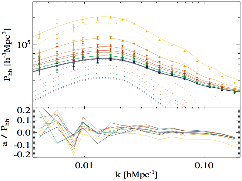
We further tests this model by comparing this model with Hamaus et al. (2010), we found that our simple method fits the non-linear power-spectrum derived from cosmological simulations quite well even up to . In Figure 5, we plot the non-linear power-spectrum from numerical simulations of halos (points with errorbars), while the solid lines are power-spectrum of various halo mass bins calculated using our simple model , the model fits the non-linear power-spectrum quite well over a significant range in k even when we have not yet added the additional constant term a. The dashed lines show the results without the shot noise term for various halo mass bins. Our model of non-linear power-spectrum is based on HALOFIT (Smith et al., 2003), so in order to not confuse the reader, we will call by . The lower panel shows the ratios between and are plotted as lines. The non-linear bias is fairly well fit by our simple model even if we do not include the extra constant bias term. We decided to include the extra constant term a to help remove the residual difference between and .
3.3.2 Non-linear effects on the BAO
We test the effect on our results of non-linear evolution on the smearing of the BAO feature by assuming that the non-linear matter power spectrum follows the expression in Eisenstein et al. (2007):
| (13) | |||||
where Mpc, is the linear theory power-spectrum (which includes the BAO) and is a smooth power spectrum, with the same shape as but without any baryonic oscillations; which is computed using the approximation described in Eisenstein & Hu (1998). Both the wiggle and the no-wiggle part have been computed in linear theory; we then added to both of them the corresponding nonlinear ratios as a function of the scale. This approach significantly enhances the power in small scales. We find that the results are not very sensitive to the exact value of provided that it is in the range of 5.527 to 9.527 Mpc (Eisenstein et al., 2007). In principle, is cosmology dependent, and thus can change our cosmological constraint if it is kept as a free parameter. We have therefore examined our constraints on cosmological parameters using different . We test this issue by fitting the full set of cosmological parameters using MCMC fitting method with COSMOMC with set to higher and lower than its currently chosen value (7.527), and find that when we fit for a CDM model in combination with WMAP7, there is less than change for any of the parameters.
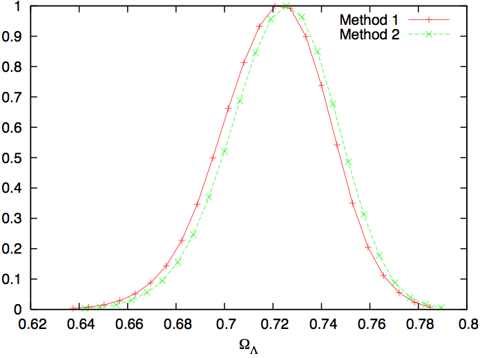
However, the addition of the nonlinear ratios is quite important, not only because the power in small scales in the angular power spectrum at high multipoles is not expected to be accounted for the shot noise due to finite number of galaxies, but also because the small shift in the BAO wiggles can slightly modify the best-fit shape of the power spectrum and hence return a different value of . We applied two different methods in calculating the power-spectrum (including the BAO) with non-linear effects taken into account, and find that it makes essentially no difference (see Figure 6).
3.4. Optimal Estimation of Angular Power Spectrum
The theory behind optimal power spectrum estimation is now well established, so we limit ourselves to details specific to this discussion, and refer the reader to the numerous references on the subject (Hamilton, 1997; Seljak, 1998, and references therein). We also refer the reader to the Appendix A for more specific details that relate to our paper directly.
We start by parametrizing the power spectrum with twenty step functions in , ,
| (14) |
where the are the parameters that determine the power spectrum. We form quadratic combinations of the data,
| (15) |
where is a vector of pixelized galaxy overdensities, is the covariance matrix of the data, and is the derivative of the covariance matrix with respect to . The covariance matrix requires a prior power spectrum to account for cosmic variance; we estimate the prior by computing an estimate of the power spectrum with a flat prior and then iterating once. We also construct the Fisher matrix,
| (16) |
The power spectrum can then be estimated, , with covariance matrix .
We also refer the reader to Appendix A for details more specific to our project.
3.5. Tests with simulations
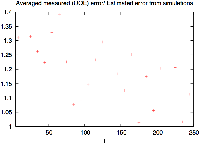
To test whether the errors estimated by the quadratic estimator employed here are accurate or not and to test the results of our pipeline, we must compute the errors obtained via a series of simulations.
One way to do this is to generate Gaussian random field using the prior power spectra for each redshift slice to simulate over the entire sphere. We can Poisson distribute galaxies with probability over the survey region, trimmed with the angular selection function. Padmanabhan et al. (2007) has tested this pipeline with the Gaussian random fields simulations, thus what we need to test here is whether the errors estimated by the quadratic estimator are appropriate, considering that the power-spectrum measurement is only minimum variance measurement when the field is Gaussian, which is not the case here. Given the non-gaussianity of the field, we need to determine how close we are to minimum variance measurement.
As we would like to simulate our galaxy sample as closely as possible, we employed CMASS mock catalogs from White et al. (2011) to test the accuracy of the optimal quadratic estimator. White et al. (2011) has produced a series of mock catalogs that use the best-fit HOD models from White et al. (2011), and populate a series of N-body simulations (White et al., 2011). The majority of the galaxies are central galaxies living in halos of mass . We generate 8 lines of sight from each corner of each of the 20 independent CMASS simulations from White et al. (2011). These mock catalogs are then processed the same manner as the real data through the quadratic estimator code, and analyzed in the same manner as the real data set. The mock angular power-spectra are thus optimally estimated angular power-spectra.
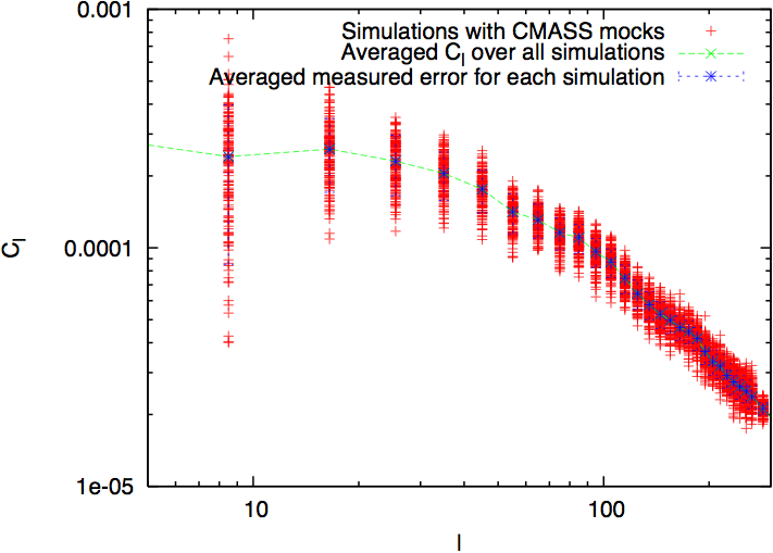
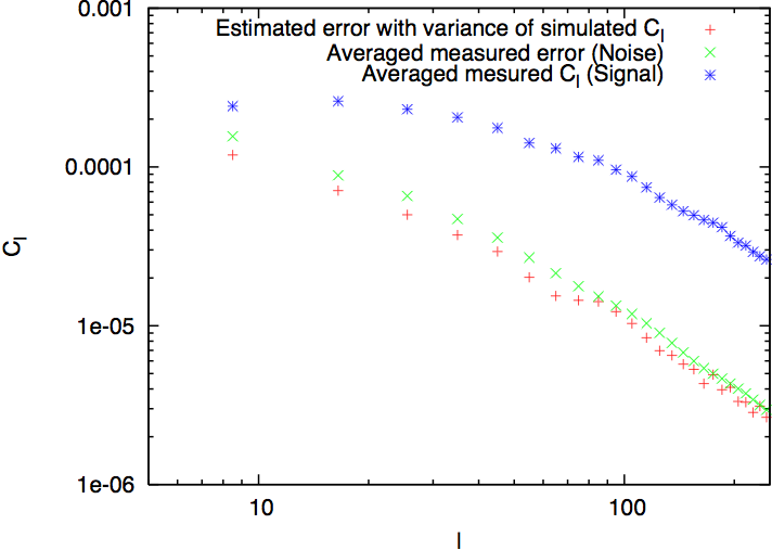
We plotted the distribution of the power-spectrum from each simulation that are estimated by the quadratic estimator code, and compare these results to the averaged error-bar of the simulation (see Figure 7). When comparing the expected error to the distribution of estimated power-spectrum from each simulation and the averaged measured error from each simulation, we conclude that the averaged measured error is a good measure of the expected error. We have plotted the estimated error (red crosses of the middle panel of Figure 7) by examining the variance of the estimated power-spectrum from each simulation at each -mode. We have also plotted the averaged measured error (green points), and it is a bit higher than the estimated error from the variance of the simulations (bottom panel). This is probably due to the fact that since there are only 20 simulation boxes, with 8 lines-of-sights overlapping slightly in within each box. Therefore, the variance of simulated is probably slightly smaller than it should be at all scales, due to the correlations between lines of sight. Regardless, we show that the quadratic estimator code can estimate the errors of the power-spectrum in the scale of interest here with reasonably high accuracy. It is important to note that at all scales of interest (to the current paper), the estimated error from the quadratic estimator code is not under-estimated.
3.6. The Optimally Estimated Angular Power Spectrum
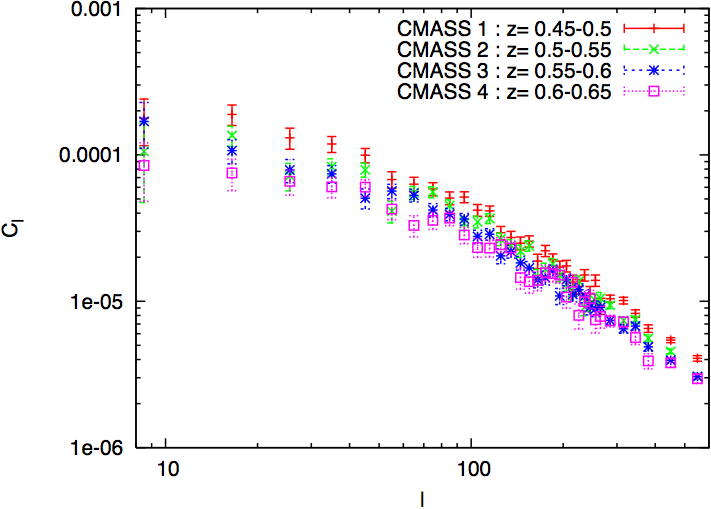
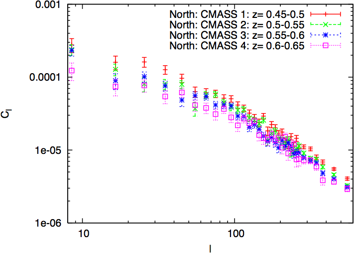
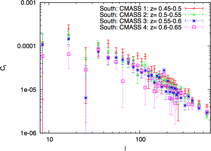
The angular power-spectra estimated using the methodology described in Sec 3.4 are displayed in Figure 8. In particular, we plot separately the north (Galactic), south and full angular power-spectra of these 4 redshift bins (CMASS 1-4, from ). We plotted the north and south separately to investigate possible systematic differences due to the long separation of observation time between north and south galactic caps. For the scales of interest (), the north and south are not different to prompt separate analyses. Nevertheless, this does not preclude possibility of systematic differences at the largest scales (at low multipole) in the angular power-spectrum. This is only possible, since the estimated power in each -bin is not correlated, therefore a systematic difference in one -bin does not affect another.
To test the similarity of north and south region on scales of interest ( ), we find all best fit cosmology parameters (with combined with WMAP7, via MCMC chain using COSMOMC) found by north and south alone respectively are consistent with each other. It is interesting to note that the south has smaller area than the north, and thus there are less information per l-bin, thus the error-bars in the south is significantly larger than the north. It will also be discussed later in Sec 4 as the systematic treatment presented in this paper will in principle correct systematic variations even when the full survey is analyzed in one piece. We can also see the evolution of the angular power-spectra over different redshift slices, as it is expected.
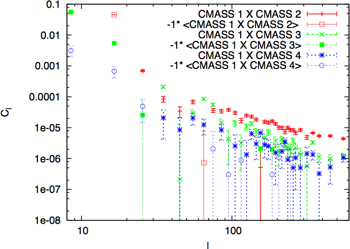
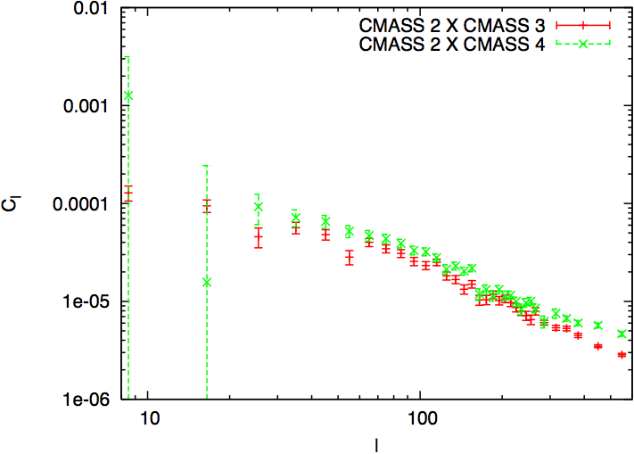
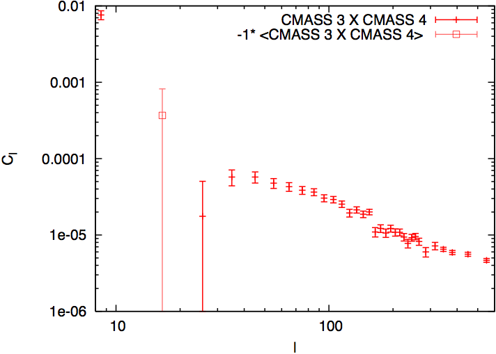
As shown in Figure 3, we need to investigate the potential effects of overlapping redshift distributions. We calculate the cross-power of various redshift combinations, and they are shown in Figure 9. Cross-power between different redshift bins not only add information in terms of cosmology, but also from the perspective of systematics.
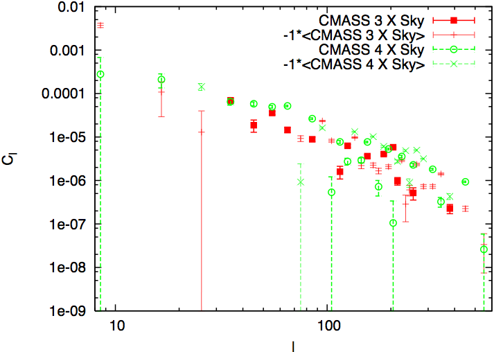
When we examine cross-power across various redshift bins, any difference between the measured power and the expected power (from galaxy auto-correlations in the same redshift range) can be used as a measure of the effects of systematics. In the top panel, there is significant extra power at large scale, and also negative correlations (which cannot come from galaxy auto-correlations), therefore, we know that there is significant systematics within CMASS 1. The bottom panel shows that the high redshift slice CMASS 4 also has substantial effects from systematics.
Finally, to estimate whether it is worth including the cross-power of various redshift slices into the cosmological analysis, we performed a simple Fisher analysis. We calculated Fisher matrices using angular spectra from the four redshift bins (CMASS 1-4), with the redshift distributions given in Figure 3. A standard CDM cosmology is employed to calculate the fiducial spectra. We used the Limber approximation (where the input power spectrum was given by CAMB 999http://camb.info/ linear power-spectrum and HALOFIT) and ignored redshift space distortions. We employ the standard Gaussian expression for the covariance matrix of the spectra. The shot noise term was calculated assuming = (with being the number of galaxies per steradian of the individual bin). Finally, to construct the Fisher matrix, we used the range . The parameter space is given by: ,, , , , , , , and ( refers to biases of galaxy sample at redshift slice N). The Fisher matrix is then added to WMAP7 Fisher matrix and invert to find the covariance matrix for the parameters. We then consider two cases: (1) using only the auto-spectra as observables and (2) using both auto- and cross-spectra as observables. The errors on all parameters improve by less than 5% in going from (1) to (2). We also found that ignoring covariances between different auto-spectra (we do include the covariance between auto power-spectra in the analysis) makes less than 5% difference. This suggests that when we include these covariances in the MCMC, the errors will not change significantly. We therefore adopt a conservative approach where we don’t include the cross-power as extra signal, but we include the bin-to-bin covariance that can, in principle, be double-counted due to the overlap of redshift slices.
4. Potential Sample Systematics
Without accurately addressing known potential systematics on the observed number density of objects in our sample, we cannot claim to understand its expected angular power-spectra, nor can we extract cosmological information from it. The treatment of systematics is especially crucial for the overall shape of power-spectrum, since the shape does not deviate much from power-laws, and has no specific features such as those in BAO. The oscillatory nature of the BAO signal helps it from being contaminated by any systematic signal that doesn’t have oscillatory features. Moreover, most BAO detection methods attempt to minimize any influence from the shape directly (Eisenstein et al., 2007), thus further shielding the BAO technique from any systematic effects. We will propose a novel method of systematic corrections in Sec 5 which helps mitigate the effects in power-spectrum caused by any systematics.
4.1. Description of Systematics
Here we consider not only sample systematics, but in particular the systematics that may contribute to extra (or deficit) power in the angular scale under consideration.
4.1.1 Stellar contamination and obscuration
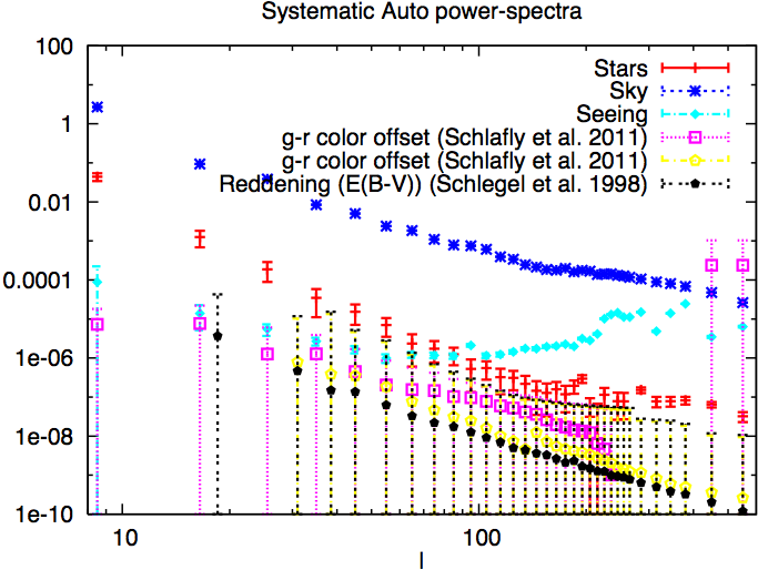
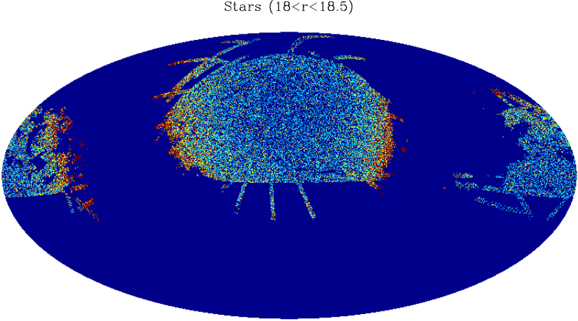
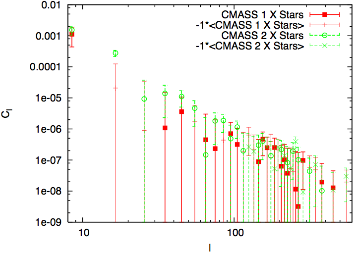
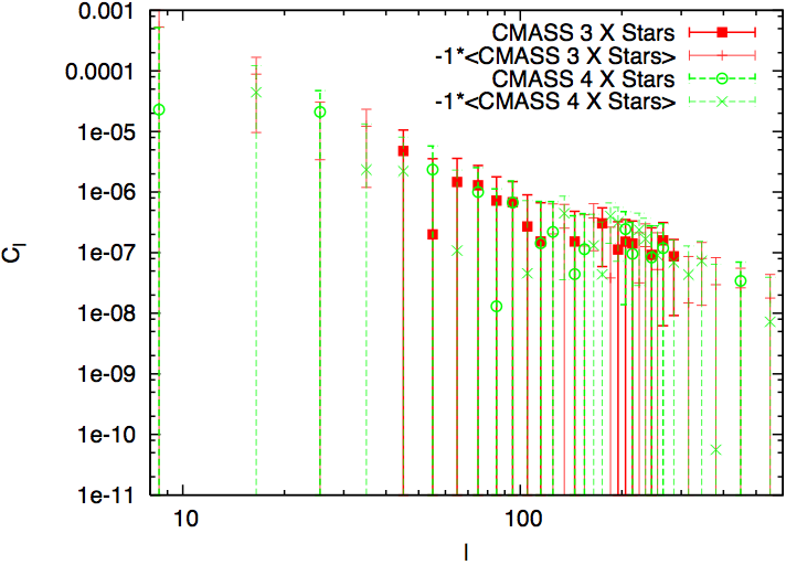
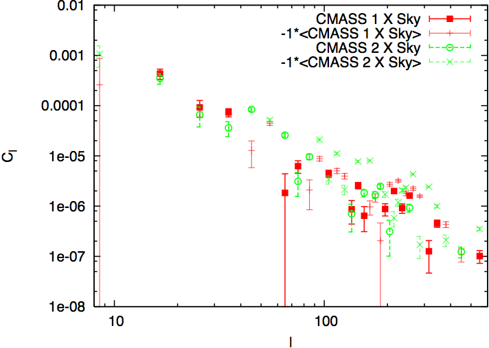
Stars can in principle mimic galaxies given the right colors, or give rise to obscuration due to possible foreground subtraction issues due to presence of a star. As it was pointed out in Ross et al. (2011) that the magnitude range of stars do not change its effect on the galaxy number density, we pick stars of magnitude , and investigate its influence on the galaxy auto power-spectrum. The stellar density map is plotted in Figure 11, while its auto power-spectrum is plotted in Figure 10. We use the same mask as the CMASS samples, since the stars can only affect the galaxy power-spectrum where the two overlap. We calculate the cross-power-spectra between the stars and the various CMASS redshift slices, and find that there is a significant correlation at several angular scales (see Fig 12), mostly at large scales. In particular, there are strong angular correlations ( for CMASS 1, for CMASS 2) between stars and the galaxies at large scales, while we observe the number of density of galaxies is lower when it is closer to a star (as also discussed in Ross et al. (2011)).In the paper, we do not include scales that are smaller than since it is much larger than the scales we are interested in this paper. However, we will discuss more for the larger scales in a future publication on primordial non-gaussianities as the largest angular scales contain more information concerning primordial non-gaussianities.
There is an extensive discussion on the stellar contamination in the CMASS catalog in Ross et al. (2011).The fundamental conclusions are that there are two separate effects: 1) stars can be confused as galaxies, thereby contaminating the sample and inducing a positive correlation between the densities of stars and our sample and 2) the presence of a star artificially reduces the chances of detecting a galaxy, thereby imparting a negative correlation. In Ross et al. (2011), since the band powers are highly correlated across bins of separating distances, the two effects together impart a slightly negative correlation between the number density of stars and our sample. In our analysis detailed in this paper, the estimated angular power-spectra are designed to have minimal correlation across bins, therefore, we can see both positive and negative correlations over different scales (-bin), as seen in Figure. 12. Given that we know stars are likely to contribute to the observed number densities, we can take into account of the amount of contamination by using the above discussed technique. Our results are consistent with Ross et al. (2011) even though we do not detect smaller scale correlations between the stars and the galaxies, since the estimator employed in this paper produces estimates of angular band powers that are minimally correlated with other bins of band powers, while estimates are highly correlated across bins in the analysis of Ross et al. (2011). Therefore, although the correlations between stars and galaxies concentrated in the largest scales, they appear in smaller angular scale such as those seen in Ross et al. (2011).
4.1.2 Sky brightness
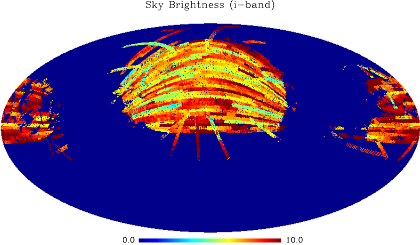
The sky brightness from SDSS is presented in Figure 13. There are at least two scales that the sky brightness would affect the expected number of galaxies. The first is the width of the scan of the SDSS camera, the second comes from the fact that the southern cap has brighter sky, since we observe the south at higher zenith angle, thus more re-emission from the optically thin lines that were pumped by the sun originally.
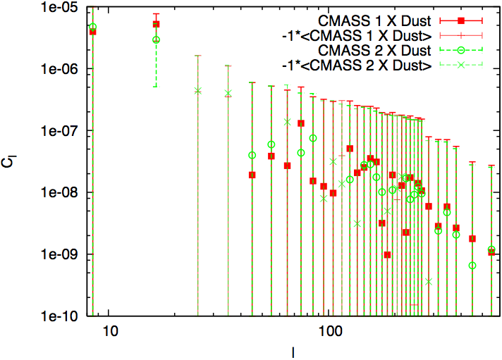
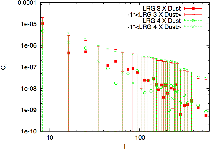
We use the auto power-spectrum of the sky brightness (shown in Figure 10), and its cross-correlations with galaxy densities at various redshifts (shown in Figure 14), to estimate the amount of contamination that can come from the sky. We discuss the corrections applied arising from sky brightness in Section 5.
4.1.3 Seeing Variation
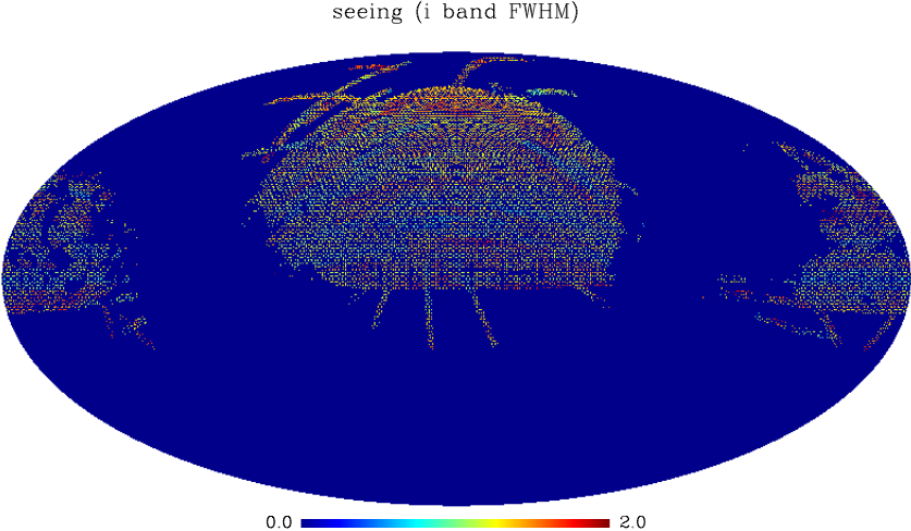
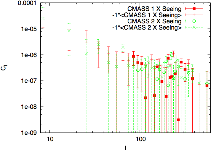
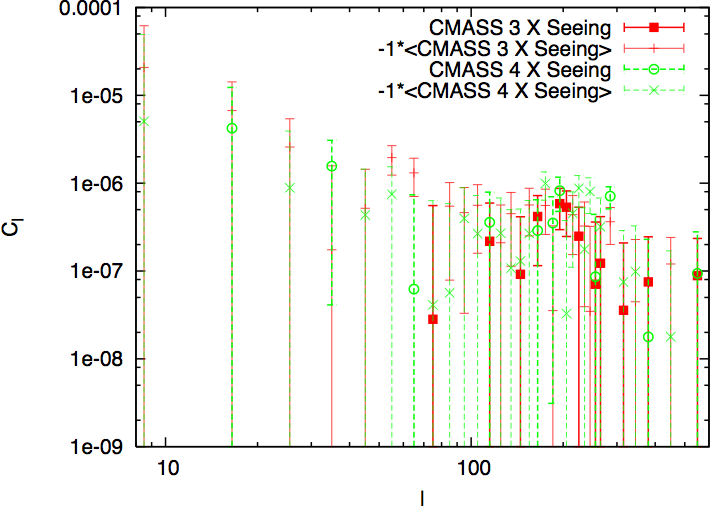
Since SDSS uses a ground-based telescope at Apache Point Observatory, it is expected that the image quality, primarily atmosphere seeing will affect the number of galaxies detected in any part of the sky. To quantify this, we plotted the seeing variations in the sky in Figure 15. There is a striped pattern as different parts of the sky are observed in different nights, which have different atmosphere seeing. We use the auto power-spectrum of the seeing variations and its cross-correlations with the galaxy density to determine the effects of seeing on the galaxy overdensity clustering power. Since we can see that there are statistically significant but mild cross-correlations between the galaxies and seeing in several of angular band power, we correct for the seeing variations as discussed in Section 5
4.1.4 Extinction
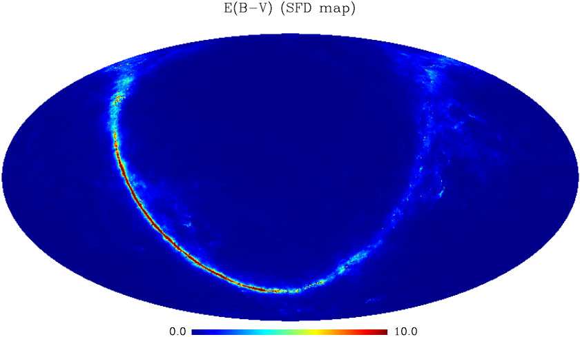
We check for any residual effects on the observed galaxy over-densities due to Galactic extinction by computing the cross-correlations between the galaxy overdensities and the extinction map (Schlegel et al., 1998) (see Figure 17). Since SDSS avoids most heavily extincted areas, we only have a small overlapping area where there is significant extinction, and galaxy data. We do not see a statistically significant cross-correlation between the galaxy (except for scale of < of CMASS 1) and the extinction field, therefore, we conclude that we will drop the galactic extinction from the list of possibly contributing systematic effects as long as the range of interest in this analysis remain smaller than > .
4.1.5 Color offsets
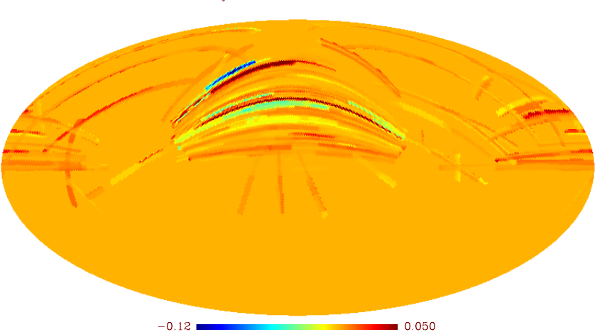
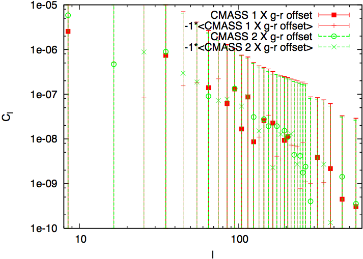
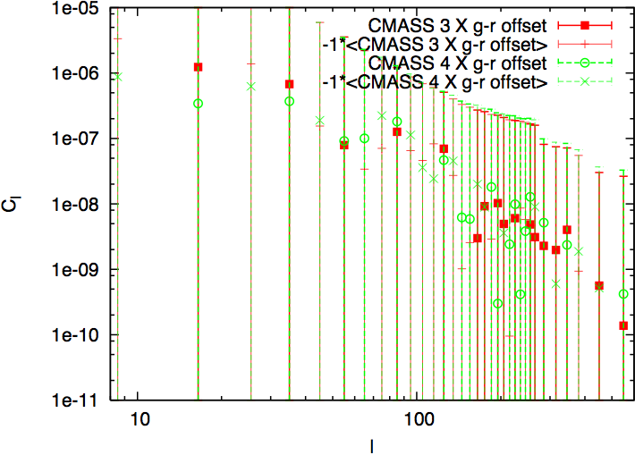
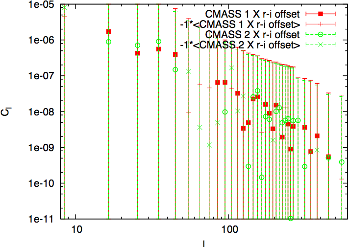
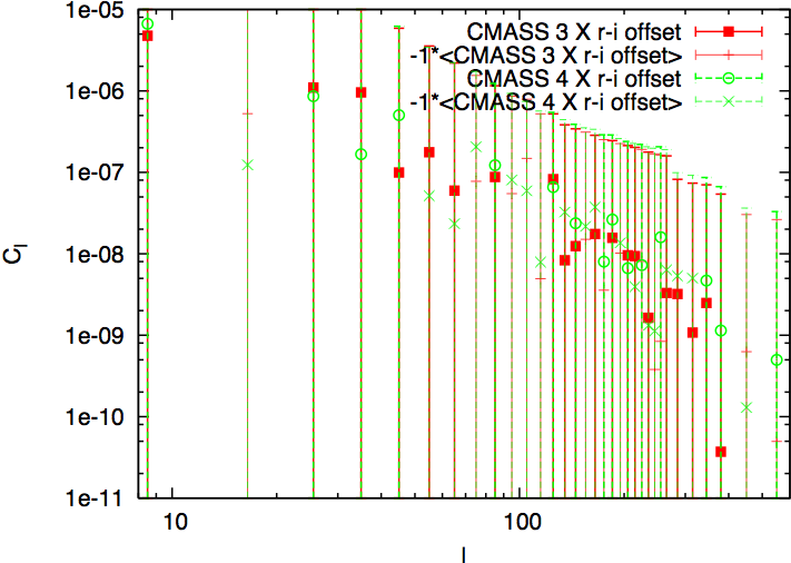
Schlafly et al. (2010) reported various color offsets for the SDSS footprint, in particular a north/south offset. As discussed in Schlafly et al. (2010), the photometric offsets can be estimated via two different ways: 1) using the color of stars in the imaging data; 2) using the stellar spectra to determines spectral classes, and then calculate differences between the observed and expected colors of stars. We adopted the later method, since it will not be sensitive to the intrinsic variations of stellar properties. However, this approach requires spectroscopy of stars, which is lacking in significant parts of SDSS southern sky. We still pursues it though, and found that there are no significant detection between the galaxy density map that overlaps with the offset map (which is lacking in southern sky coverage). We therefore conclude that this is not an important systematics in our sample. However, this is only a statement that at the sky which are overlapped between the galaxy density map and the offset map, there isn’t significant correlations. We will need more data in terms of the southern sky offsets before we can conclude on the effects of color offsets and galaxy densities.
.
4.1.6 Magnitude Errors
As mentioned in Ross et al. (2011), the model magnitude errors in the southern cap are larger than the northern cap by , this may introduce a possible power excess (or deficit) at the lowest multipole. This issue however shouldn’t affect any of the other multipoles which are the focus of our paper.
5. Novel Treatment of Systematics
Assuming that residual systematics will exist best catalog we can construct without a serious loss of sky, how should we handle the remaining systematics? Without any evidence of possible non-linear effects of systematics on the observed density fields, we adopt the simplest approach: linear relationship between the systematics and the observed galaxy density fields.
We start from the following: Transforming fields from real space into spherical harmonic space (or l space in particular), so that :
| (17) |
where is the true galaxy density (in the -space), and each is the fluctuations of the map of the i-th systematic, while characterizes how much i-th systematic contributes. With the lack of a better model, we assumes a linear relationship between the systematics and the observed galaxy number overdensity, but in principle this model can be modified to include higher order contamination due to the systematics.
For a simple demonstration, we consider that we have only two systematics contributing to the observed galaxy density, so that . Assuming that the true galaxy density is unrelated to any of our systematics, we have the following:
| (18) |
Furthermore, we have all the cross-correlations between the systematic and the observed galaxy density map:
| (19) |
and
| (20) |
Since we calculate all the auto- and cross- correlations of all the systematics (on top of the cross-correlations between the systematics and the observed galaxy density), we can solve for and (and they will be functions of ).
In Figure 21, we show the cross-correlations of all the systematics (which contaminates the observed galaxy field), we find that the correlations across different systematics are far from zero, and we must include the cross-correlations among systematics in our model.
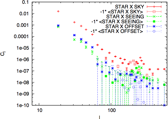
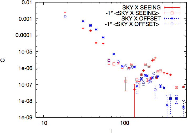
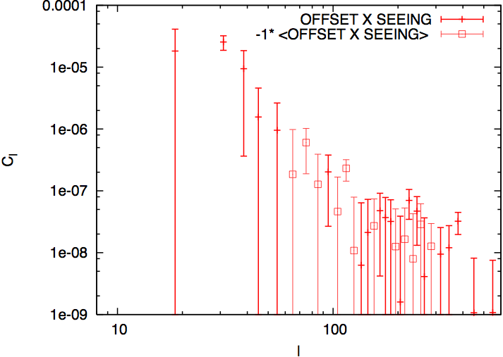
For simplicity of demonstration, we show the application of applying the correction from only 1 systematic (stars) in Figure 22. Since there is only inclusion of 1 systematic, the correction depends only on the auto-power of the stars and the cross-correlation between the stars and the observed density field. Although star is one of our dominant systematics, its effect on scales of interest ( > 30) are quite minimal. This implies that with the appropriate estimator (which do not correlate powers in various scales), effects from systematics can be corrected relatively easily. This result further encourages us in terms of the cosmological constraining power that can be harnessed from future imaging surveys that will go deeper and wider.
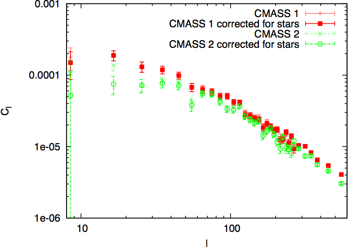
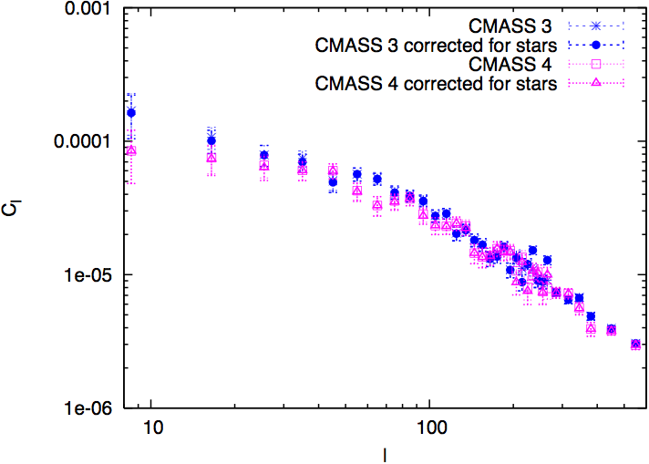
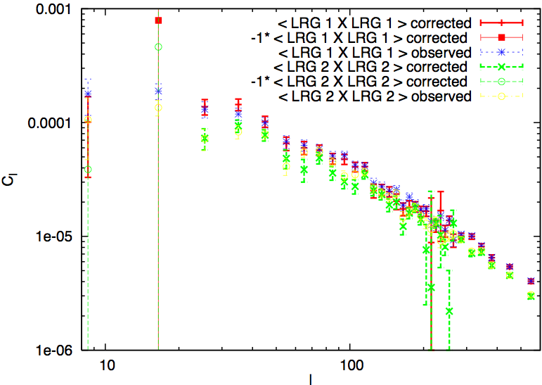
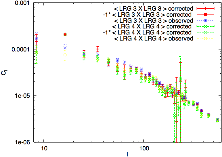
Finally, we calculate the final systematic-corrected power by including all three systematics which are found to have significant correlations with the observed galaxy density field. We include the auto-power (of both systematics and galaxy density fields) and all cross-powers (among systematics and galaxy fields) at each angular scale. The final corrected power is shown in Figure 23.
Nevertheless, as the optimal quadratic estimator produces optimal errors and unbiased measurement only when the field is gaussian. In the case of highly non-Gaussian fields, the estimate is still unbiased, but the error is not optimal and may not be accurate. We can only test the validity of estimated error by the quadratic estimator if we simulate a large number of systematic mocks, and carry out variance tests such as the ones carried out for the galaxy density fields.
While we understand the construction of mock galaxy catalogs, we do not fully understand how to construct mock systematic fields. We lack the ’theory’ of systematics fields (except probably the stellar density map). Therefore, it is unlikely that we can achieve optimal error on the systematic corrections within the scope of this analysis. The estimated values is unbiased, but the error can be over-estimated or maybe incorrect (Hamilton, 1997). Nonetheless, when the systematic corrections are small, the uncertainty related to the correction cannot be larger than the correction itself. Therefore, we conclude that the most conservative way would be to include only power from multipoles that have relatively small corrections. Lacking a better model for the systematics, we adopt the following simplistic model of estimating the covariance of the systematic-corrected power-spectra for multipole bins which require small corrections. We assume Gaussianity of the fields involved, and thus using the following relationship:
| (21) |
We modify the above equation by adding the ”correctional power” due to systematics:
| (22) |
This is for each , so we take into account the fact that the is not 1 in all of our bins. The quantity is the correctional power contribued by systematics. This method assumes the gaussianity of the fields, which is not a satisfactory assumption, the optimal quadratic estimator can in principle project out powers that are understood, such as those time-dependent systematics can be projected out in the CMB map-making. Nonetheless, a full modeling of the systematics and then projecting them out using optimal quadratic estimator is a much larger under-taking, which will be left to future work.
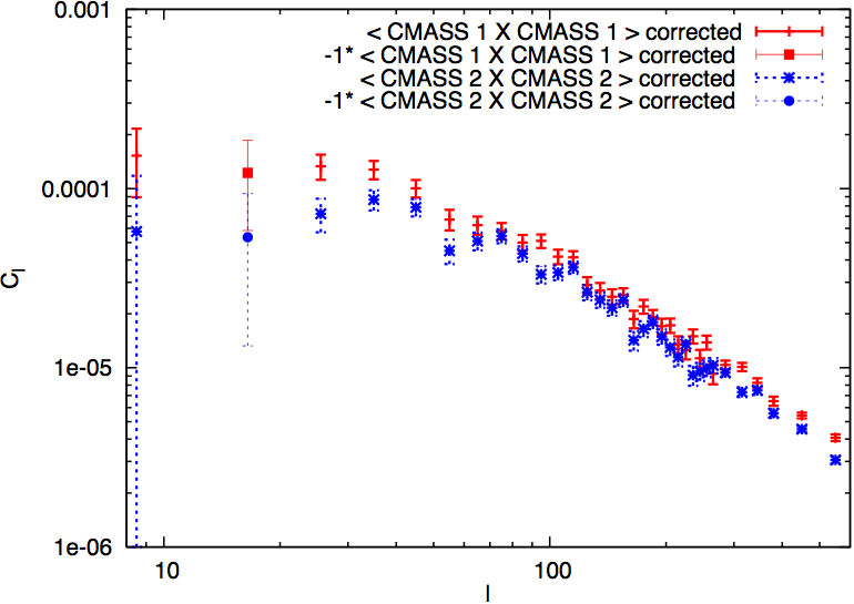
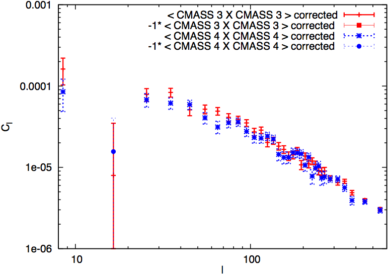
We also show for completeness purposes the power-spectra of various redshift slices before and after the corrections in Figure 24.
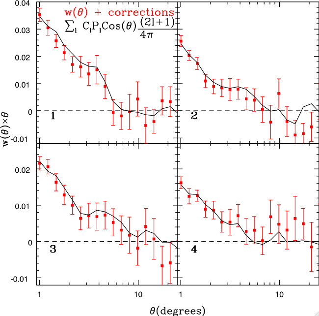
We also compute the correlation function of our systematic corrected power-spectra and compare with those presented in Ross et al. (2011) and found that they are completely consistent with each other after systematic corrections. One of the systematic correlation correction method employed in Ross et al. (2011) follows our paper 101010Even though this analysis is submitted at a later date, the Ross et al. (2011) paper is part of the DR8 clustering project in SDSS III, and thus Ross et al. (2011) has applied our method described here., and thus it is not surprising that we have achieved the same systematically corrected correlation function, even though the computation of the correlation function is independent. The figure 25 shows how our computed correlation function from our systematically-corrected optimally-estimated angular power-spectra is completely consistent (to within ) with the measurement of Ross et al. (2011). We would also note that our correlation function shown in black lines in Figure 25 (our calculated using the angular power-spectra) has no significant large scale power, which suggests no exotic inflation scenario, nor residual systematics.
6. Cosmological Parameter Fitting Method and Validation
6.1. Method
As described in Sec 3.3, we adopt the simple linear redshift-independent biasing model (with shot noise subtracted for every single angular power-spectra). Therefore, in addition to the cosmological parameters that are of interest for each model, we include three extra parameters for each redshift slice (, and ) as shown in 8.
We have estimated that the non-linear redshift space distortion effects are minimal in our case (Saito et al., 2012), therefore we include the full linear redshift space distortion following Padmanabhan et al. (2007) as discussed in Sec.3.2. However, calculating the full linear redshift space distortions requires significant time, and it is different from Limber approximation at ; therefore, we made a decision to employ Limber approximation for multipole ranges at , and employing the full linear redshift space distortion calculation only at .
The measured band powers from the quadratic estimator have contributions from a range of wave numbers, even though they are highly concentrated in their own -bin. The quadratic estimator is designed to compute nearly anti-correlated power spectra (Padmanabhan et al., 2003) across different multipole bins, but it still has a very small () contribution from other multipole bins. We take this effect into account by convolving the theory power-spectra with the window function before calculating the likelihood by , where represents the measured power-spectra, represents the theory power-spectra convolved with window function and is the covariance across different bands and redshifts as output from the quadratic estimator.
The fitting of the all cosmological parameters are done through MCMC with COSMOMC (Lewis & Bridle, 2002). As it was discussed earlier, we do not know the accuracies of the error estimated using a highly non-Gaussian field with quadratic estimator. We know that it won’t be biased, but the error-bar can be significantly mis-estimated. When the systematic corrections are small, we can assume that the error involved with the correction cannot be significant. However, at the largest angular scales, some of the systematic corrections are large enough that only proper error propagation that involves significant undertaking in full modeling of systematics would provide sufficient accuracy on the error of the correction. There are also concerns about the validity of the assumption of linear effects of systematics on the galaxy density field, especially when the corrections are large. We do not have indications to believe that the effects of systematics on galaxy density field is linear or non-linear. Therefore, we decided to avoid the scales that involve large systematic corrections, which are concentrated at the large scales, thus setting the start of the multipole range from .
Since our data-set is a photometric sample, the non-linear effects are mitigated by the fact that when we examine the data-set, it is already integrated along all line-of-sights, thus decreasing its non-linearities. We therefore apply the HALOFIT routine for computing the non-linear power-spectrum, and limit ourselves to multipoles that are at relatively large scale, while non-linearities remain a small effect. We choose the multipole range by simply testing variety of ranges using our simulations described in Sec 3.5. In order for MCMC chain of the simulation to converge quickly, we average the simulations across different simulation boxes (so that they are not correlated). We tested a large range of multipole ranges: , , , for example, and found and to return results within 1-sigma of the input parameters. It is also of interest to show the corresponding -limit for the various ranges, since the range in may provide an easier reference for the non-linearities of interest. We list the corresponding range for the range we use for the redshift bins considered in our analysis in Table 2.3.
Combining both the low and the high limit, we conclude that and are both conservative choices for fitting of cosmological parameters.
6.2. Cosmological Parameter Fitting Method Validation
In this Section we present some of the tests used to check -likelihood routine for COSMOMC. To perform such a test we need an angular power spectrum whose input cosmology (i.e. the cosmological model with which was generated, modulo cosmic variance) is completely known. Therefore, the mock angular power spectrum described in Section 3.4, being derived from a cosmological simulation with initial conditions given by a known set of values for the cosmological parameters, provides an excellent testbed for our fitting routine.
The most straightforward test is to fit each individual angular power spectrum from the mocks and check that every one of them (out of the 160 available) returns the input cosmology. However, running 160 MCMC chain with only one mock power-spectra each is computationally intensive, especially since each angular power-spectra has the power of actual redshift slice from the data, thus it will take significant time for the chains to converge if they converge at all.
We therefore need to combine these mock with additional data-set, and the most obvious choice being the CMB data from WMAP7 (Larson et al., 2011). The WMAP7 best fit parameters however are not exactly the same as the simulation input parameters, thus we replace the standard CMB-likelihood by a much simpler one, in which we compute the value of from the actual covariance matrix from WMAP7, but not using the actual parameters themselves. To fully validate the fitting method, we need to use mocks that show a similar signal-to-noise ratio as those observed in the data. We combine individual mocks by using different simulations (and not different lines of sight in the same simulation).
6.2.1 Building Covariance of mocks
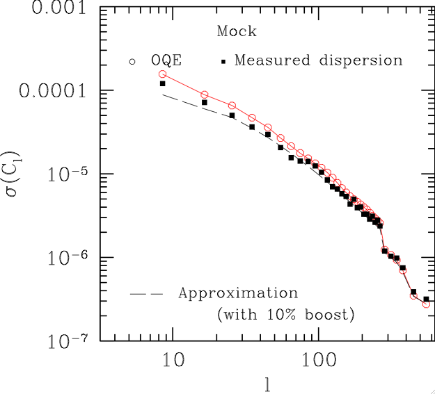
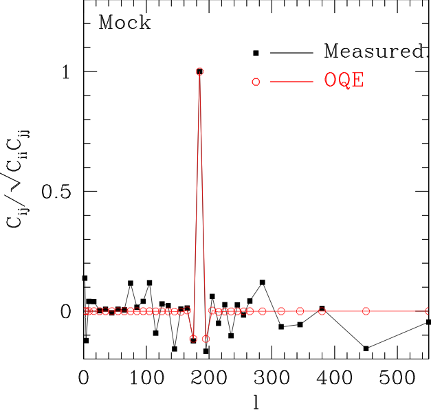
We compare the Gaussian covariance matrix of power spectrum from OQE (i.e., ‘OQE covariance matrix’) with the dispersions among 160 mocks (i.e., N-bodycovariance matrix’). Note that the 160 mocks are not strictly independent from each other, as different lines of sight share a small but nonzero amount of volume. To exclude the artificial covariance between different lines of sight, we derive the covariance matrix of the 20 independent mocks per each line-of-sight; we then average the eight covariance matrices for eight lines of sight. As a comparison, a straightforward dispersion among 160 mocks gives an almost identical result, implying that the different lines-of-sight share very little volume.
In the upper panel of Figure 26, the red points are square roots of the diagonal elements of the OQE covariance matrix, and the black squares are from the N-body covariance matrix. The diagonal elements of the OQE covariance matrix can be analytically calculated based on the smooth fit to the measured power spectrum and the number of independent modes for each wave number band assuming Gaussianity, if the matrix is diagonal. However, the OQE covariance matrix includes the effect of the window function due to the survey geometry, and the covariance matrix therefore is not strictly diagonal and has a small anti-correlation between neighboring bins. Indeed, we find that there is a small deviation between the OQE covariance matrix and a naive Gaussian error calculation without accounting for the window function. The difference is expected since the naive Gaussian error calculation does not include the effects of the actual survey geometry. The black dashed lines in the figure are the theoretical, expected error derived based on Gaussianity; we have rescaled it with an empirical boost factor of 1.1 to better match the observed dispersion. The dispersions between mocks are systematically lower than the OQE on large scales but appears to lie between the OQE expectation and the boosted Gaussian apprixomation.
The lower panel shows the off-diagonal elements of the N-body covariance matrix in comparison to the OQE covariance, for a slice at . We observe fluctuations up to 20% in the measured off-diagonal terms but find no obvious indication that it disagrees with the OQE covariance matrix. Therefore, we conclude that the OQE covariance matrix based on the Gaussian assumption does not underestimate the true error of the 2-dimensional projection of the nonlinear galaxy field.
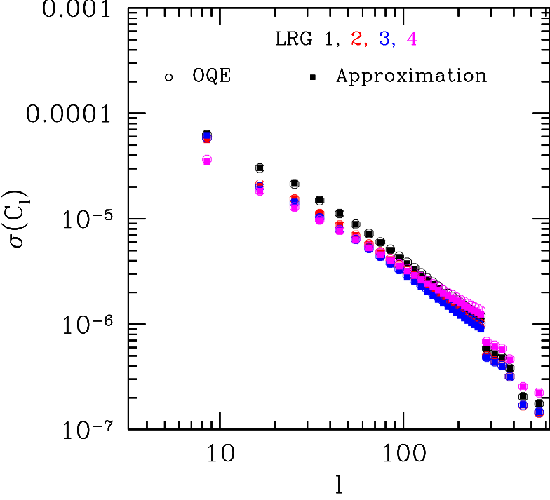
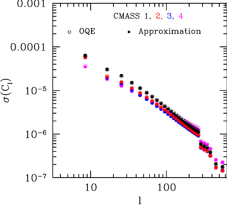
For the real data, we use the covariance matrix from the OQE for the auto-power for each redshift bin.; while we use the OE The upper panel of Figure 27 shows the square roots of the diagonal elements of the OQE covariance matrix of the real data (open circles) in comparison to the prediction based on the Gaussian prediction (after boosted by 1.1: solid squares) for all four redshift bins. The agreement is even better than the mock case, and it is probably due to the larger survey area of the real data that decreases the cross-correlation between different bins that our simple Gaussian approximation cannot access. The lower panel shows the cross-correlation between different bins for four different slices of the OQE covariance matrix. We overplot covariance matrices for CMASS1 (black), CMASS2 (red), CMASS3 (blue), and CMASS4 (magenta). Note that the covariance structure is identical for the four redshift bins, which is reasonable as the four redshift bins are subject to the same mask. The same structure should apply to the covariance between different redshift bins as well. We therefore build the cross-covariance between different redshift bins by combining the diagonal elements from the Gaussian assumption and the covariance structure in the right panel of Figure 27. The diagonal elements are constructed using smooth fits to the measured auto and the cross-power spectra of and between redshift bins and boosted by 1.1 based on the results of the auto power spectra:
| (23) |
where and indicates a redshift slice, is the fraction of the sky, is the number of wave modes within the band, and is a smooth fit to the auto or cross power spectrum; we include the shot noise contribution to in the case of the auto power spectra (i.e., ). The factor is the empirical factor of 1.1 that we introduce to match the OQE covariance matrix and equation 23. We use this equation to build the covariance between different redshift slices, while using the OQE covariance matrix for the covariance within the redshift slice.
6.2.2 Mock test results
With the combined average of 20 spectra each in combination with the pseudo-WMAP7, we find that the above model recovers all input cosmological parameters of the CMASS mocks for all 8 averaged power-spectra to within . The recovered bias parameters are also very similar to the input bias of the CMASS mocks as described in White et al. (2011). We therefore conclude that this model accurately recovers cosmological parameters when used in the range of angular scale specified above.
7. Results
7.1. Constraints on Cosmological Models
The angular clustering measurement can be used to constrain cosmological model in several different ways: through standard rulers such as the matter-radiation turn-over scale, the baryon acoustic oscillations, or through large scale power which would constrain primordial non-gaussianities (Dalal et al., 2008; Slosar et al., 2008). In companion paper (Seo, 2011), we examine only baryon acoustic oscillations, and remove any contribution from the overall shape of the power-spectrum; in this paper, we include the overall shape of the power-spectrum and parts of the baryon acoustic oscillations to derive constraints on cosmological models. There is a companion publication on the neutrino mass constraints using the same angular power-spectrum (de Putter et al., 2011).
Here, we choose to consider a variety of cosmological models, although not intending to exhaust all possibilities. We include several other data-sets to help break cosmological degeneracies, such as WMAP7 (Larson et al., 2011), the “Union 2” supernova dataset (hereafter SN), which includes 557 supernova from Hamuy et al. (1996); Riess et al. (1999); Riess et al. (2007); Astier et al. (2006); Jha et al. (2006); Wood-Vasey et al. (2007); Holtzman et al. (2008); Hicken et al. (2009); Kessler et al. (2009), and constraints from using 600 Cepheids observed by Wide Feild Camera 3 (WFC3) published by Riess et al. (2011) (HST).
7.1.1 Flat CDM model with a constant equation of state
We investigate the flat CDM model with a constant equation of state parameter () to characterize Dark Energy with the combination of our angular power-spectra from SDSS-III Data Release 8 (DR8) with other data-sets. When we combine our DR8 observed angular power-spectra with WMAP7 +HST + SN dataset, we find , and (see Fig 28). We also combine our systematic-corrected DR8 angular power-spectra with WMAP7 +HST +SN data-set, we find , . The systematically-corrected angular power-spectra gives consistent results compared with the observed angular power-spectra.
We compare our results with other large scale structure datasets, such as the latest large scale structure constraints from galaxy clustering in Blake et al. (2010), which has detected BAO at using spectroscopic survey WiggleZ which includes 200,000 galaxy spectra over 800 . They found a similar constraints on the equation of state of dark energy: when they combined with WMAP7 + SN. This implies that our dataset, even though it is purely imaging data, gives a similar constraining power when compared to latest spectroscopic survey such as WiggleZ.
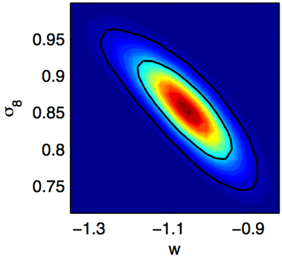
We also compare our results with the BAO constraints from SDSS-DR7, when combined with WMAP7 + HST (Reid et al., 2010; Percival et al., 2010), they found , while Montesano et al. (2011) used full shape of P(k) from SDSS-DR7, when they combined it with CMB + HST, they found . When we combine with the same dataset (CMB+HST), we find , which implies that our dataset gives a similar constraining power as with the full 3D DR7 spectroscopic sample (at ), while our purely imaging dataset is at a higher redshift range (0.45-0.65).
7.1.2 Open CDM model
For an open CDM model, when combined with WMAP7+HST, we find , improving the accuracy over the WMAP7 +HST constraints on by ( from WMAP7+HST); see Fig 29.
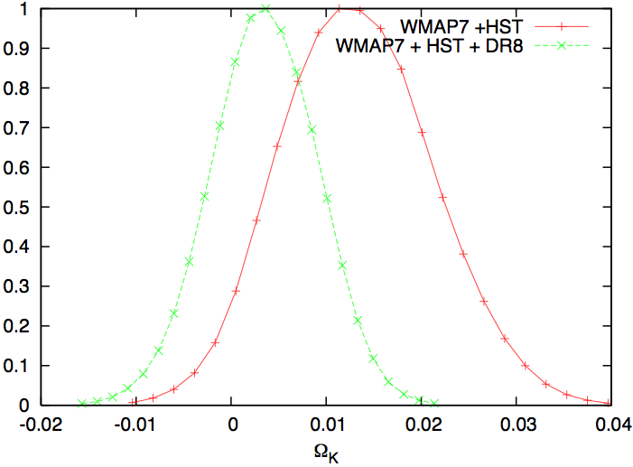
When we compare our measurement to other large scale structure measurements such as DR7-BAO constraints; we find very similar constraints; for example, on as WMAP7+HST+DR7 gives .
7.1.3 Flat CDM model
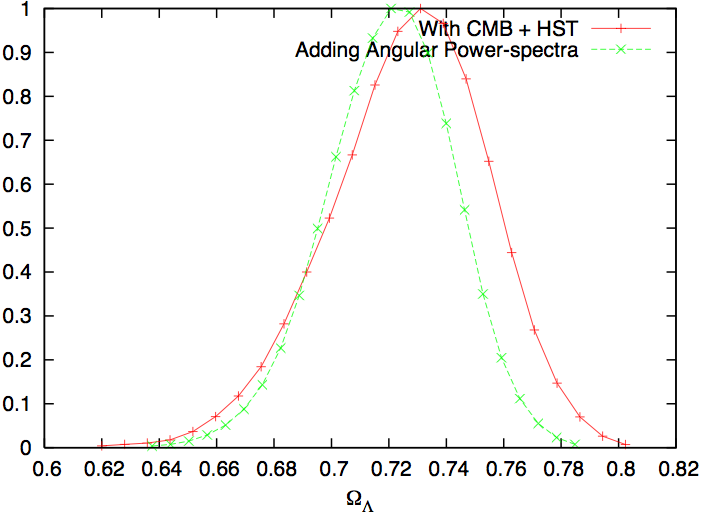
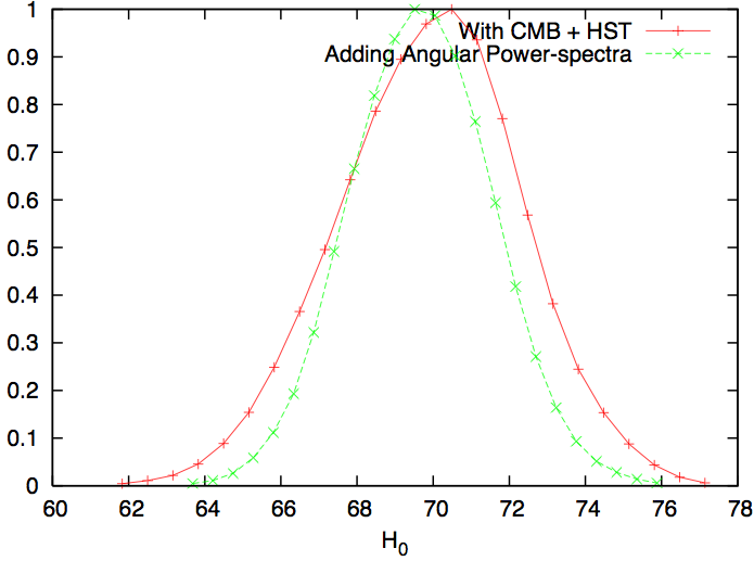
For a flat CDM model, when combined with WMAP + HST, we find , to be and to be , which are consistent with WMAP+HST only, while improving the accuracy over just WMAP+HST by for all parameters. We show the improvement on cosmological constraining power over the combination of WMAP7 and HST in Figure 30.
7.2. Companion Results
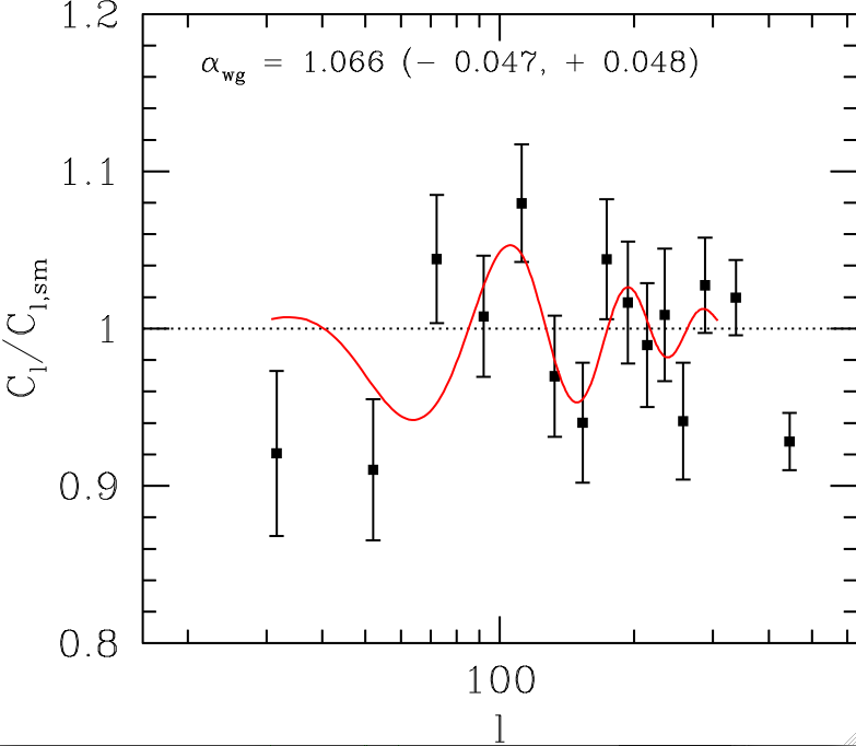
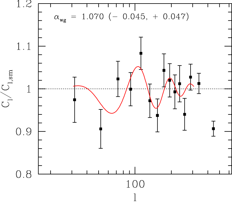
In this paper, we are utilizing the full power spectum over , including both the broadband shape and the BAO. As a comparison, our companion paper Paper II, Seo et al. (2011) derives the angular diameter distance scale using the BAO feature over as a standard ruler, while excluding nearly all the non-BAO information. To summarize their method and result, they use the angular power spectra and the covariance matrix shown in this paper, build a reasonable template power spectra based on the estimated, true galaxy distribution as a function of redshift and the concordance cosmology, and fit for the distance scale, while marginalizing over many free parameters that account for the shape of the broad band. They derive at and the result is shown to be robust against assumptions they make during the fitting process. Figure 31 summarizes the BAO fits they derived before and after the systematics correction.
In a second companion paper, de Putter et al. (2011), the angular spectra discussed in the present paper are are used to derive a strong new upper bound on the sum of neutrino masses. As neutrinos suppress growth of structure on scales above the neutrino free streaming length, they leave a characteristic signature in the power spectra. To exploit this signal, de Putter et al. (2011) model the galaxy spectra and their neutrino mass dependence, test the model using mocks and show that it can be safely applied to the multipole range , while also considering the conservative range . The angular clustering galaxy data are then combined with priors from WMAP7, the HST Hubble parameter measurement, supernova distances and the (low redshift) SDSS BAO measurement and the resulting upper bounds are discussed. We quote here the conservative bound, from DR8+CMB+HST+BAO+SN, of eV at CL, and refer the reader to the article itself for more details.
8. Conclusion and Discussion
We have measured the 2D clustering power spectrum of luminous red galaxies using the SDSS-DR8 photometric survey. The principal results of this analysis are summarized and discussed below.
Using photometric redshifts, we constructed a large uniform sample of galaxies between redshifts to . This probes a cosmological volume of , making this the largest cosmological volume ever used for a galaxy clustering measurement. The large volume allows us a measurement of power going from the smallest scales to the largest. In particular, we probe all the way from the smaller scales such as the Baryon Acoustic Oscillations scale out to the scale of matter-radiation equality with one of the most accurate measurement of angular clustering at achieved to date.
We applied a novel approach of treating systematics by incorporating both the cross/auto-power of systematics with themselves and cross-power with galaxies. This allows us to not only understand the impact of various systematics on observed galaxy number densities, but also allows applcation of small corrections at scales where the corrections are small, thus the uncertainty related to the corrections are negligible. Since we choose only scales that are minimally affected by systematics, we expect the final cosmological constraints from both pre-/and post-systematic corrections are consistent with each other, which is indeed the case. This method can be improved drastically by two extra components, which will be left to future work. First, we should be able to project out the appropriate modees that are contributed by the systematics in similar way as it is done in CMB map-making (Stompor et al., 2002), and this can be done when one is estimating the optimally estimated power-spectra. Second, we should be able to model the distribution of the systematics (for example, whether it is gaussian or not) by investigating multi-epoch data that is available in SDSS-DR8. In particular, this is available in the Stripe 82 area, which even though small (in comparison to DR8 full foot-print), it contains square degrees which were multiply scanned ( repeats for each fields). This will allow us to estimate the undertainty of our systematic corrections properly. These two components will significantly improve not only our understanding of the systematics, thus allowing us to push our analysis to include larger angular scales (which are affected by the systematics more significantly). However, both of them requires significant undertakings in both data collection, code development and simulations, while the improvements will not dramatically change our cosmological interpretation in this paper, therefore, we leave these two components for future projects.
For a flat CDM model, combining our data with WMAP7 + HST, we find and to be . For a open CDM model, when combined with WMAP7 + HST, we find , improved over WMAP7+HST alone by . For a wCDM model, when combined with WMAP7+HST+SN, we find , and to be , which is competitive with the latest large scale structure constraints from spectroscopic surveys such as those by WiggleZ (Blake et al., 2010), and SDSS DR7 spectroscopic surveys, especially in analysis led by (Reid et al., 2010; Percival et al., 2010; Montesano et al., 2011). This results implies that our dataset, even though it is purely imaging data, possesses a similar constraining power as the spectroscopic surveys such as WiggleZ or SDSS-DR7. What we lack in redshift precision, we compensate by shear volume. This suggests that future and upcoming imaging surveys such as PanStarrs 111111http://pan-starrs.ifa.hawaii.edu/public/, DES 121212http://www.darkenergysurvey.org/science/index.shtml and LSST 131313http://www.lsst.org can achieve significant cosmological constraints via large scale structure clustering even when compared to other spectroscopic surveys.
This is the Paper I of the project, which mostly describes the construction of the data-set, treatment of systematics, estimation of the angular power-spectra and finally using the overall shape of the angular power-spectra over a large range of angular scale to derive constraints on our cosmological models. We refer readers to Paper II (Seo, 2011) of the project, which uses only the Baryon Acoustic Oscillation feature to fit for various cosmological parameters. We also refer to Paper III (de Putter et al., 2011) of the project, which uses the overall shape of the power-spectra to fit for various neutrino models.
9. Acknowledgment
We would like to thank Nico Hamaus for testing our treatment for non-linearities using N-body simulations, Pat McDonald for fruitful discussion on our systematic treatments and Uros Seljak for useful discussions. S.H. would like to acknowledge Martin White for all the useful discussions and encouragement even though he is already a co-author. S.H. would also like to thank UC Berkeley, Department of Energy and Lawrence Berkeley National Laboratory for ther support through Seaborg and Chamberlain Fellowship. This work was supported by the U.S. Department of Energy under Contract No. DE-AC03-76SF00098 and in part by the facilities and staff of the Yale University Faculty of Arts and Sciences High Performance Computing Center. This research used resources of the National Energy Research Scientific Computing Center, which is supported by the Office of Science of the U.S. Department of Energy under Contract No. DE-AC02-05CH11231. Funding for SDSS-III has been provided by the Alfred P. Sloan Foundation, the Participating Institutions, the National Science Foundation, and the U.S. Department of Energy Office of Science. The SDSS-III web site is http://www.sdss3.org/.
SDSS-III is managed by the Astrophysical Research Consortium for the Participating Institutions of the SDSS-III Collaboration including the University of Arizona, the Brazilian Participation Group, Brookhaven National Laboratory, University of Cambridge, Carnegie Mellon University, University of Florida, the French Participation Group, the German Participation Group, the Instituto de Astrofisica de Canarias, the Michigan State/Notre Dame/JINA Participation Group, Johns Hopkins University, Lawrence Berkeley National Laboratory, Max Planck Institute for Astrophysics, New Mexico State University, New York University, Ohio State University, Pennsylvania State University, University of Portsmouth, Princeton University, the Spanish Participation Group, University of Tokyo, University of Utah, Vanderbilt University, University of Virginia, University of Washington, and Yale University.
References
- Abazajian et al. (2004) Abazajian K., Adelman-McCarthy J. K., Agüeros M. A., et al., 2004, AJ, 128, 502
- Aihara et al. (2011) Aihara H., Allende Prieto C., An D., et al., 2011, ApJS, 193, 29
- Astier et al. (2006) Astier P., Guy J., Regnault N., et al., 2006, A&A, 447, 31
- Blake et al. (2010) Blake C., Brough S., Colless M., et al., 2010, MNRAS, 406, 803
- Blanton et al. (2003) Blanton M. R., Lin H., Lupton R. H., et al., 2003, AJ, 125, 2276
- Bond & Efstathiou (1984) Bond, J. R., & Efstathiou, G. 1984, ApJ, 285, L45
- Carlson et al. (2009) Carlson J., White M., Padmanabhan N., 2009, Phys. Rev. D, 80, 4, 043531
- Cole et al. (2005) Cole S., Percival W. J., Peacock J. A., et al., 2005, MNRAS, 362, 505
- Collister & Lahav (2004) Collister, A. A., & Lahav, O. 2004, PASP, 116, 345
- Dalal et al. (2008) Dalal, N., Doré, O., Huterer, D., & Shirokov, A. 2008, Phys. Rev. D, 77, 123514
- de Putter et al. (2011) de Putter R., Mena O., Guisarma, E., Ho, S., et al. 2011, submitted in conjunction
- Driver et al. (2009) Driver, S. P., Norberg, P., Baldry, I. K., et al. 2009, Astronomy and Geophysics, 50, 050000
- Eisenstein & Hu (1998) Eisenstein D. J., Hu W., 1998, ApJ, 496, 605
- Eisenstein et al. (1999) Eisenstein D. J., Hu W., Tegmark M., 1999, ApJ, 518, 2
- Eisenstein et al. (2005) Eisenstein D. J., Zehavi I., Hogg D. W., et al., 2005, ApJ, 633, 560
- Eisenstein et al. (2007) Eisenstein D. J., Seo H.-J., White M., 2007, ApJ, 664, 660
- Eisenstein et al. (2011) Eisenstein, D. J., Weinberg, D. H., Agol, E., et al. 2011, AJ, 142, 72
- Firth et al. (2003) Firth, A. E., Lahav, O., & Somerville, R. S. 2003, MNRAS, 339, 1195
- Fukugita et al. (1996) Fukugita M., Ichikawa T., Gunn J. E., Doi M., Shimasaku K., Schneider D. P., 1996, AJ, 111, 1748
- Gorski et al. (1999) Gorski K. M., Wandelt B. D., Hansen F. K., Hivon E., Banday A. J., 1999, ArXiv Astrophysics e-prints
- Groth (1973) Groth E. J., 1973, in Sixth Texas Symposium on Relativistic Astrophysics, edited by D. J. Hegyi, vol. 224 of Annals of the New York Academy of Sciences, 184–+
- Gunn et al. (1998) Gunn, J. E., Carr, M., Rockosi, C., et al. 1998, AJ, 116, 3040
- Gunn et al. (2006) Gunn J. E., Siegmund W. A., Mannery E. J., et al., 2006, AJ, 131, 2332
- Hamaus et al. (2010) Hamaus N., Seljak U., Desjacques V., Smith R. E., Baldauf T., 2010, Phys. Rev. D, 82, 4, 043515
- Hamilton (1997) Hamilton A. J. S., 1997, MNRAS, 289, 295
- Hamilton (1993) Hamilton, A. J. S. 1993, ApJ, 417, 19
- Hamilton & Tegmark (2004) Hamilton, A. J. S., & Tegmark, M. 2004, MNRAS, 349, 115
- Hamuy et al. (1996) Hamuy, M., Phillips, M. M., Suntzeff, N. B., et al. 1996, AJ, 112, 2398
- Heitmann et al. (2009) Heitmann, K., Higdon, D., White, M., et al. 2009, ApJ, 705, 156
- Hicken et al. (2009) Hicken M., Wood-Vasey W. M., Blondin S., et al., 2009, ApJ, 700, 1097
- Ho et al. (2008) Ho S., Hirata C., Padmanabhan N., Seljak U., Bahcall N., 2008, Phys. Rev. D, 78, 4, 043519
- Ho et al. (in prep) Ho S., Myers A., et al. (in prep)
- Høg et al. (2000) Høg E., Fabricius C., Makarov V. V., et al., 2000, A&A, 355, L27
- Holtzman (1989) Holtzman, J. A. 1989, ApJS, 71, 1
- Holtzman et al. (2008) Holtzman, J. A., Marriner, J., Kessler, R., et al. 2008, AJ, 136, 2306
- Hu (1999) Hu W., 1999, ApJ, 522, L21
- Hu & White (1996) Hu, W., & White, M. 1996, ApJ, 471, 30
- Huchra et al. (1983) Huchra, J., Davis, M., Latham, D., & Tonry, J. 1983, ApJS, 52, 89
- Ilbert et al. (2006) Ilbert, O., Arnouts, S., McCracken, H. J., et al. 2006, A&A, 457, 841
- Jha et al. (2006) Jha S., Kirshner R. P., Challis P., et al., 2006, AJ, 131, 527
- Kessler et al. (2009) Kessler R., Becker A. C., Cinabro D., et al., 2009, ApJS, 185, 32
- Koo (1998) Koo, D. C. 1998, Highlights of Astronomy, 11, 468
- Larson et al. (2011) Larson D., Dunkley J., Hinshaw G., et al., 2011, ApJS, 192, 16
- Le Fèvre et al. (2005) Le Fèvre, O., Vettolani, G., Garilli, B., et al. 2005, A&A, 439, 845
- Lewis & Bridle (2002) Lewis, A., & Bridle, S. 2002, Phys. Rev. D, 66, 103511
- Lupton et al. (2001) Lupton R., Gunn J. E., Ivezić Z., Knapp G. R., Kent S., 2001, in Astronomical Data Analysis Software and Systems X, edited by F. R. Harnden Jr., F. A. Primini, & H. E. Payne, vol. 238 of Astronomical Society of the Pacific Conference Series, 269–+
- Maddox et al. (1990) Maddox, S. J., Efstathiou, G., Sutherland, W. J., & Loveday, J. 1990, MNRAS, 243, 692
- Masters et al. (2011) Masters K. L., Maraston C., Nichol R. C., et al., 2011, MNRAS, 1417
- Montesano et al. (2011) Montesano, F., Sanchez, A. G., & Phleps, S. 2011, arXiv:1107.4097
- Padmanabhan et al. (2003) Padmanabhan, N., Seljak, U., & Pen, U. L. 2003, New Astronomy, 8, 581
- Padmanabhan et al. (2008) Padmanabhan N., Schlegel D. J., Finkbeiner D. P., et al., 2008, ApJ, 674, 1217
- Padmanabhan et al. (2007) Padmanabhan N., Schlegel D. J., Seljak U., et al., 2007, MNRAS, 378, 852
- Peebles & Yu (1970) Peebles, P. J. E., & Yu, J. T. 1970, ApJ, 162, 815
- Peebles (1973) Peebles P. J. E., 1973, ApJ, 185, 413
- Peebles (1980) Peebles P. J. E., 1980, The large-scale structure of the universe
- Percival et al. (2010) Percival W. J., Reid B. A., Eisenstein D. J., et al., 2010, MNRAS, 401, 2148
- Pier et al. (2003) Pier J. R., Munn J. A., Hindsley R. B., et al., 2003, AJ, 125, 1559
- Reid et al. (2010) Reid B. A., Percival W. J., Eisenstein D. J., et al., 2010, MNRAS, 404, 60
- Reid & White (2011) Reid B. A., White,M. [arXiv:1105.4165 [astro-ph.CO]].
- Riess et al. (1999) Riess, A. G., Kirshner, R. P., Schmidt, B. P., et al. 1999, AJ, 117, 707
- Riess et al. (2007) Riess A. G., Strolger L.-G., Casertano S., et al., 2007, ApJ, 659, 98
- Riess et al. (2011) Riess A. G., Fliri J., Valls-Gabaud D., 2011, ArXiv e-prints
- Ross et al. (2006) Ross, A. J., Brunner, R. J., & Myers, A. D. 2006, ApJ, 649, 48
- Ross et al. (2011) Ross A. J., Ho S., Cuesta A. J., et al., 2011, MNRAS, 1393–+
- Saito et al. (2012) Saito, S., White, M., Ho, S. (in prep)
- Sánchez et al. (2008) Sánchez, A. G., Baugh, C. M., & Angulo, R. 2008, MNRAS, 390, 1470
- Sánchez et al. (2009) Sánchez, A. G., Crocce, M., Cabré, A., Baugh, C. M., & Gaztañaga, E. 2009, MNRAS, 400, 1643
- Schlafly et al. (2010) Schlafly E. F., Finkbeiner D. P., Schlegel D. J., et al., 2010, ApJ, 725, 1175
- Schlegel et al. (1998) Schlegel D. J., Finkbeiner D. P., Davis M., 1998, ApJ, 500, 525
- Scoccimarro (2004) Scoccimarro, R. 2004, Phys. Rev. D, 70, 083007
- Scoville et al. (2007) Scoville N., Abraham R. G., Aussel H., et al., 2007, ApJS, 172, 38
- Scranton et al. (2002) Scranton, R., Johnston, D., Dodelson, S., et al. 2002, ApJ, 579, 48
- Seljak (1998) Seljak U., 1998, ApJ, 506, 64
- Seljak & McDonald (2011) Seljak, U., & McDonald, P. 2011, arXiv:1109.1888
- Seo (2011) Seo H-J., Ho, S., White, M., Cuesta, A., et al. 2011, submitted in conjunction
- Skrutskie et al. (2006) Skrutskie, M. F., Cutri, R. M., Stiening, R., et al. 2006, AJ, 131, 1163
- Slosar et al. (2008) Slosar, A., Hirata, C., Seljak, U., Ho, S., & Padmanabhan, N. 2008, Journal of Cosmology and Astroparticle Physics, 8, 31
- Smith et al. (2002) Smith J. A., Tucker D. L., Kent S., et al., 2002, AJ, 123, 2121
- Smith et al. (2003) Smith, R. E., Peacock, J. A., Jenkins, A., et al. 2003, MNRAS, 341, 1311
- Stompor et al. (2002) Stompor, R., Balbi, A., Borrill, J. D., et al. 2002, Phys. Rev. D, 65, 022003
- Stoughton et al. (2002) Stoughton C., Lupton R. H., Bernardi M., et al., 2002, AJ, 123, 485
- Sunyaev & Zeldovich (1970) Sunyaev, R. A., & Zeldovich, Y. B. 1970, Ap&SS, 7, 20
- Swanson et al. (2008) Swanson, M. E. C., Tegmark, M., Blanton, M., & Zehavi, I. 2008, MNRAS, 385, 1635
- Taruya et al. (2010) Taruya, A., Nishimichi, T., & Saito, S. 2010, Phys. Rev. D, 82, 063522
- Tegmark et al. (2004) Tegmark M., Blanton M. R., Strauss M. A., et al., 2004, ApJ, 606, 702
- Thomas et al. (2011) Thomas, S. A., Abdalla, F. B., & Lahav, O. 2011, Physical Review Letters, 106, 241301
- Wang et al. (1999) Wang Y., Spergel D. N., Strauss M. A., 1999, ApJ, 510, 20
- White et al. (2011) White M., Blanton M., Bolton A., et al., 2011, ApJ, 728, 126
- Wood-Vasey et al. (2007) Wood-Vasey W. M., Miknaitis G., Stubbs C. W., et al., 2007, ApJ, 666, 694
- York et al. (2000) York, D. G., Adelman, J., Anderson, J. E., Jr., et al. 2000, AJ, 120, 1579
- Zehavi et al. (2002) Zehavi, I., Blanton, M. R., Frieman, J. A., et al. 2002, ApJ, 571, 172
Appendix A Quadratic Estimator
Consider a Gaussian random field with and covariance
| (A1) |
We wish to form an estimator, , of which is quadratic in the data
| (A2) |
where is symmetric. Requiring the estimator to be unbiased
| (A3) |
For Gaussian the covariance of is
| (A4) |
This problem is easiest if we consider a single parameter at a time, with all other parameters held fixed (and absorbed into ). Thus we wish to minimize
| (A5) |
Taking derivatives with respect to the components of gives
| (A6) |
or
| (A7) |
If the dependence of on is not linear then we can use a Newton-Raphson iteration where now is the derivative of evaluated at the current best value of . Iterating, by replacing until the best-fit , results in a maximum likelihood solution. In practice, it only takes a few iterations to achieve the maximum likelihood solution.
This approach also results in another fact that is under-appreciated in the literature. The above choice of (which can have a slightly different form, see Table 4 of Padmanabhan et al. (2003) for more details) produce error-bars that are anti-correlated across different band powers. In this paper, we include the window function (which is mostly affected by the mask) before we compare the observed power and the theoretical power.