Simulation of Asymptotically AdS₅ Spacetimes with a Generalized Harmonic
Evolution Scheme

Abstract

Motivated by the gauge/gravity duality, we introduce a numerical scheme based on generalized harmonic evolution to solve the Einstein field equations on asymptotically anti-de Sitter (AdS) spacetimes. We work in global AdS₅, which can be described by the $(t,r,\chi,\theta,\phi)$ spherical coordinates adapted to the $\mathbb{R}\times S^{3}$ boundary. We focus on solutions that preserve an $SO(3)$ symmetry that acts to rotate the 2-spheres parametrized by $\theta,\phi$. In the boundary conformal field theory (CFT), the way in which this symmetry manifests itself hinges on the way we choose to embed Minkowski space in $\mathbb{R}\times S^{3}$. We present results from an ongoing study of prompt black hole formation via scalar field collapse, and explore the subsequent quasi-normal ringdown. Beginning with initial data characterized by highly distorted apparent horizon geometries, the metrics quickly evolve, via quasi-normal ringdown, to equilibrium static black hole solutions at late times. The lowest angular number quasi-normal modes are consistent with the linear modes previously found in perturbative studies, whereas the higher angular modes are a combination of linear modes and of harmonics arising from non-linear mode-coupling. We extract the stress energy tensor of the dual CFT on the boundary, and find that despite being highly inhomogeneous initially, it nevertheless evolves from the outset in a manner that is consistent with a thermalized $\mathcal{N}=4$ SYM fluid. As a first step towards closer contact with relativistic heavy ion collision physics, we map this solution to a Minkowski piece of the $\mathbb{R}\times S^{3}$ boundary, and obtain a corresponding fluid flow in Minkowski space.

I Introduction

It has been hoped since the beginnings of the AdS/CFT correspondence, first formulated in Maldacena (1998); Gubser et al. (1998); Witten (1998), that gauge-gravity dualities would eventually be used to relate gravitational calculations to experimentally testable predictions in gauge theory. Over the past several years, there has been a flurry of activity in applying AdS/CFT to problems in high energy and condensed matter physics, which began with the discovery of the strongly-coupled quark-gluon plasma formed in heavy ion collisions. Recent proposals have suggested application to other systems, including those that exhibit superconductivity, the quantum hall effect, and superfluidity. For some review articles see Gubser and Karch (2009); Herzog (2009); Hartnoll (2009); McGreevy (2010); Sachdev (2010); Gubser (2010a); Horowitz (2010); Gubser (2011). Though conformal field theories cannot model the exact properties of all of these physical phenomena, it is hoped that they nevertheless capture aspects of the essential physics. In the strong coupling limit of the boundary CFT, the duality maps CFT states to bulk gravity configurations, and there are many cases where the latter theory is more tractable than the former. In many if not most of the model problems studied to date, the gravity description has involved black holes; aside from the interesting philosophical questions this poses, the implication is that one needs to study bulk solutions within the strong-field regime of general relativity. In situations where exact solutions are not known, or perturbative expansions about known solutions are inadequate to capture the non-linear dynamics, numerical solution of the Einstein field equations for an asymptotically AdS spacetime is required.

Numerical relativity has seen significant progress in recent years modeling dynamical, strong-field geometries, though the majority of applications have been to compact object collisions in asymptotically flat spacetimes. For some review articles see Pretorius (2007); Duez (2010); Campanelli et al. (2010); Centrella et al. (2010). The asymptotic structure of AdS is drastically different from that of flat space; in particular the boundary of AdS is time-like and in causal contact with bulk geometric structures, on time scales relevant to the boundary physics. This poses unique challenges for numerical evolution. The majority of existing literature on numerical solution in AdS has focused on black hole formation in spherically-symmetric 3-dimensional Pretorius and Choptuik (2000); Husain and Olivier (2001); Hwang et al. (2011), 4-dimensional Bizon and Rostworowski (2011), 5-dimensional Garfinkle and Pando Zayas (2011) and general $D$-dimensional Husain et al. (2003); Birukou et al. (2002) spacetimes, i.e. $1+1$ dimensional simulations where the boundary is a single point, significantly simplifying its treatment. A notable exception is a study of colliding shockwaves in 5-dimensional AdS (AdS₅), with application to heavy ion collisions Chesler and Yaffe (2011) (and see Wu and Romatschke (2011); Chesler and Teaney (2011) for follow-up studies). Planar symmetry was imposed in two spatial dimensions, reducing the problem to a $2+1$ dimensional simulation. Their approach was based on a null (characteristic) evolution scheme which is well-adapted to describing such colliding plane waves. This method simplifies the treatment of the AdS₅ boundary, though is difficult to generalize to situations with less symmetry. A more recent related study of boundary hydrodynamics via numerical solution of the full field equations in the bulk was presented in Heller et al. (2011); though the evolution was effectively $1+1$ dimensional, the space-plus-time decomposition, as used here, in principle allows for a straightforward extension to situations with less symmetry.

Inspired by the growing success of gauge/gravity dualities, we are initiating a new program to solve the Einstein field equations in asymptotically AdS₅ spacetimes, based on the generalized harmonic (GH) evolution scheme presented in Pretorius (2005a, b). These methods were introduced in the context of asymptotically flat spacetimes, and it turns out to be a rather non-trivial exercise to adapt them to AdS₅. The main purpose of this paper is to describe, in detail, the steps taken towards achieving a stable Cauchy evolution code in spacetimes that are asymptotically AdS₅. In this first study we impose an $SO(3)$ symmetry for simplicity; since the method is based on Cauchy evolution, it should be straightforward to relax this symmetry restriction for future studies, at the expense of computational complexity. As a sample application, we study the quasi-normal ringdown of initial data describing highly distorted black holes formed from scalar field collapse, and extract the stress energy tensor of the dual conformal field theory defined on the $\mathbb{R}\times S^{3}$ boundary. The $SO(3)$ symmetry we impose here is precisely the one identified in analytical studies of colliding shock waves in AdS₅ Gubser et al. (2008, 2009).

An outline of the rest of the paper is as follows. We begin in Sec. II with relevant facts about asymptotically AdS₅ spacetimes. In Sec. III, we describe a method for constructing AdS₅ initial data based on a conformal decomposition, restricted to time-symmetric initial conditions. For this study we use a scalar field to source deviations from pure AdS₅, and find that we can solve for arbitrarily strong initial data: the initial slice can be made to contain an apparent horizon, and this horizon can be made arbitrarily large by adjusting (for example) the amplitude of the initial scalar field profile. In Sec. IV, we describe the GH formalism that we use to evolve the initial data forward in time. Crucial to the stability of this scheme is the asymptotic nature of the so-called source functions that in GH evolution are traditionally associated with coordinate degrees of freedom. Here, in contrast to asymptotically flat spacetimes, we find that their asymptotic form can not be freely specified if the metric deviation is to be non-singular in the approach to the AdS₅ boundary. This and other subtleties related to evolution are clarified and addressed in the latter parts of the section. We discretize the field equations using finite difference methods, and the details of the numerical methods that we use to solve the initial data and evolution equations are discussed in Sec. V.

Results from a study of highly deformed black holes, their subsequent evolution and ringdown, and the stress tensor of the corresponding states in the dual boundary CFT, are presented in Sec. VI. What is novel about this study is that the initial horizon geometry cannot be considered a small perturbation of the final static horizon, and hence we are probing an initial non-linear phase of the evolution of the bulk spacetime. Shortly after the initial time, the metric can be described by a combination of quasi-normal modes and what appear to be gauge modes. We find frequencies that are consistent with the linear modes found in perturbative studies of static black holes, and in modes at higher angular number, we find evidence of non-linear mode-coupling. On the boundary, the dual CFT stress tensor behaves like that of a thermalized $\mathcal{N}=4$ super-Yang-Mills (SYM) fluid. We find that the equation of state $\epsilon=3P$ of this fluid is consistent with conformal invariance (here, $\epsilon$ and $P$ are the rest frame density and pressure of the fluid, respectively), and that its transport coefficients match those previously calculated for an $\mathcal{N}=4$ SYM fluid via holographic methods. Modulo a brief transient that is numerical in nature, this matching appears to hold from $t=0$ onwards. This is not a priori inconsistent with earlier results from quasi-normal modes Kovtun and Starinets (2006); Janik and Peschanski (2006); Friess et al. (2007) and numerical analyses Chesler and Yaffe (2011); Heller et al. (2011); Wu and Romatschke (2011); Chesler and Teaney (2011), where a certain “thermalization time” is observed before the boundary physics begins to correspond to that of a fluid. In contrast to those studies, we begin with a large, distorted black hole, i.e. an inhomogeneous thermal state, and the physics studied here is more of equilibration rather than of thermalization.

In the final section, we transform solutions computed in global AdS onto a Minkowski piece of the boundary, and examine the temperature of the corresponding fluid flows. Under this transformation, the spatial profile of temperature at the initial time resembles a Lorentz-flattened pancake centered at the origin of Minkowski space. By interpreting the direction along which the data is flattened as the beam-line direction, our initial data can be thought of as approximating a head-on heavy ion collision at its moment of impact.

We relegate to Appendix A some technical details on the effect of matter backreaction on the asymptotic metric fall-off. In Appendix B, we discuss how our asymptotic metric boundary conditions relate to the boundary conditions derived in Ishibashi and Wald (2004) for linearized gravitational perturbations on an AdS background that lead to well-defined dynamics, and in Appendix C we tabulate the scalar field quasi-normal mode frequencies. Throughout, we use geometric units where Newton’s constant $G$ and the speed of light $c$ are set to $1$.

II Gravity in Asymptotically AdS₅ Spacetimes

II.1 The AdS₅ Spacetime

The Lagrangian density of gravity with cosmological constant $\Lambda$, coupled to matter with a Lagrangian density $\mathcal{L}_{m}$, is given by

$$\mathcal{L}=\frac{1}{16\pi}\left(R-2\Lambda\right)+\mathcal{L}_{m},$$ (1)

where $R$ is the Ricci scalar. The corresponding equations of motion then take the local form

$$R_{\mu\nu}-\frac{1}{2}Rg_{\mu\nu}+\Lambda g_{\mu\nu}=8\pi T_{\mu\nu}.$$ (2)

Here, $R_{\mu\nu}$ is the Ricci tensor, $g_{\mu\nu}$ is the metric tensor and $T_{\mu\nu}$ is the stress energy tensor of the matter. The metric of AdS₅ is the maximally symmetric vacuum solution of (2) in $D=5$ dimensions, with a negative cosmological constant $\Lambda\equiv\Lambda_{5}<0$. In terms of the global coordinates $x^{\mu}=(t,r,\chi,\theta,\phi)$ that cover the whole spacetime, this solution is

$$ds^{2} \equiv \hat{g}_{\mu\nu}dx^{\mu}dx^{\nu}$$

$$= -f(r)dt^{2}+\frac{1}{f(r)}dr^{2}+r^{2}d{\Omega_{3}}^{2}$$

where we have defined $f(r)=1+r^{2}/L^{2}$ for convenience. Here, $d{\Omega_{3}}^{2}=d\chi^{2}+\sin^{2}\chi\left(d\theta^{2}+\sin^{2}\theta d\phi^{2}\right)$ is the metric of the 3-sphere parametrized by angles $\chi,\theta,\phi$, and $L$ is the AdS radius of curvature, related to the cosmological constant by $\Lambda_{5}=-(D-1)(D-2)/(2L^{2})=-6/L^{2}$. We are free to set the AdS length scale $L$, which is the scale with respect to which all other lengths are measured. In the code we set $L=1$, though we will continue to explicitly display $L$ in all of the following, unless otherwise indicated.

Due to the significance of the AdS₅ boundary in the context of AdS/CFT, it is useful to introduce a “compactified” radial coordinate $\rho$ so that the boundary is at a finite $\rho$. We choose

$$r=\frac{\rho}{1-\rho/\ell},$$ (4)

where $\ell$ is an arbitrary compactification scale, independent of the AdS length scale $L$, such that the AdS₅ boundary is reached when $\rho=\ell$. In our code and in all of the following, we set $\ell=1$, though note that this scale is implicitly present since $\rho$ has dimensions of length. Transforming to the $\rho$ coordinate, the metric (II.1) takes the form:

$$ds^{2}=\frac{1}{(1-\rho)^{2}}\left(-\hat{f}(\rho)dt^{2}+\frac{1}{\hat{f}(\rho)}d\rho^{2}+\rho^{2}d{\Omega_{3}}^{2}\right)$$ (5)

where $\hat{f}(\rho)=(1-\rho)^{2}+\rho^{2}/L^{2}$.

AdS₅ can also be described as the universal cover of the hyperboloid $X^{A}$ in $\mathbb{R}^{4,2}$ defined by the locus

$$-(X^{-1})^{2}-(X^{0})^{2}+\sum_{i=1}^{i=4}(X^{i})^{2}=-L^{2}.$$ (6)

This space has symmetry group $SO(4,2)$ whose transformations preserve the quadratic form (6). The metric of AdS₅ is then the metric $\hat{g}_{\mu\nu}$ induced on the above hyperboloid from the flat metric $\hat{G}_{AB}$ of an $\mathbb{R}^{4,2}$ ambient space. Here the metric $\hat{G}_{AB}$ is simply given by $\hat{G}=diag(-1,-1,1,1,1,1)$. The hyperboloid can be more efficiently described in terms of embedding coordinates $x^{\mu}$ defined by a set of embedding functions $X^{A}(x^{\mu})$, so that the induced metric $\hat{g}_{\mu\nu}$ on the hyperboloid is

$$\hat{g}_{\mu\nu}=\left(\frac{\partial X^{A}}{\partial x^{\mu}}\right)\left(\frac{\partial X^{B}}{\partial x^{\nu}}\right)\hat{G}_{AB}.$$ (7)

The global coordinates $x^{\mu}=(t,r,\chi,\theta,\phi)$ can then be thought of as corresponding to a choice of embedding functions

$$X^{-1} = \sqrt{r^{2}+L^{2}}\cos(t/L)$$

$$X^{0} = \sqrt{r^{2}+L^{2}}\sin(t/L)$$

$$X^{1} = r\sin\chi\sin\theta\sin\phi$$

$$X^{2} = r\sin\chi\sin\theta\cos\phi$$

$$X^{3} = r\sin\chi\cos\theta$$

$$X^{4} = r\cos\chi.$$ (8)

Notice that $t=0$ and $t=2\pi L$ are identified on the hyperboloid, so that there are closed time-like curves in this space. AdS₅ is defined as the hyperboloid’s universal cover precisely to remove these closed time-like curves. This universal cover is obtained by unwrapping the $S^{1}$ parametrized by $t$ on the hyperboloid, which would then run from $-\infty$ to $\infty$ in AdS₅.

II.2 Boundary of AdS₅

The boundary of AdS₅ differs dramatically from that of asymptotically flat spacetimes. To see this, let us first remember how the analogous story unfolds in the familiar setting of Minkowski space, whose metric in polar coordinates $\eta_{\mu\nu}dx^{\mu}dx^{\nu}=-dt^{2}+dr^{2}+r^{2}d\Omega^{2}$ can be rewritten through a series of coordinate transformations $u_{\pm}=t\pm r$, $\tilde{u}_{\pm}=\arctan u_{\pm}=(T\pm R)/2$ to read

$$ds^{2}=\frac{1}{4\cos^{2}u_{+}\cos^{2}u_{-}}\left(-dT^{2}+dR^{2}+\sin^{2}Rd\Omega^{2}\right).$$ (9)

Through this conformal compactification, the infinite region $t\in(-\infty,\infty)$, $r\in[0,\infty)$ is mapped to the interior of a compact region defined by $|T\pm R|<\pi$. Given that $T$ is a time-like coordinate and $R>0$ is a space-like coordinate, this region is the triangle $T\in[-\pi,\pi]$, $R\in[0,\pi]$ in the $T,R$ plane—see Fig. 1. Consequently, the boundary consists of the two null surfaces of future/past null infinity, meeting at spatial infinity. Spatial infinity in Minkowski space is thus not in causal contact with its interior. Notice that the geometry of Minkowski space is conformal to a patch $T\in[-\pi,\pi]$ of the Einstein static universe.

Figure 1: The conformal diagram of Minkowski space. The boundary consists of the point at spatial infinity $i^{0}$, and the null surfaces at future null infinity $\mathcal{J}^{+}$ and past null infinity $\mathcal{J}^{-}$. In this compactification, future time-like infinity $i^{+}$ and past time-like infinity $i^{-}$ are represented by points. Dashed lines are constant $t$ surfaces, and solid lines are constant $r$ surfaces.

The conformal compactification of AdS₅ is achieved by the spatial coordinate transformation $r/L=\tan R$, which brings its metric (II.1) into the form

$$ds^{2}=\frac{L^{2}}{\cos^{2}R}\left(-dt^{2}+dR^{2}+\sin^{2}R{d\Omega_{3}}^{2}\right)$$ (10)

where the infinite region $r\in[0,\infty]$ is mapped to the interior of a compact region $R\in[0,\pi/2]$—see Fig. 2. This halved range of $R$ implies that anti-de Sitter space is conformal to one-half of the Einstein static universe. More crucially, we have not rescaled the time coordinate $t$ in this compactification. The important consequence is a spatial infinity that runs along the $t$ direction: it is time-like and thus causally connected to the interior.

Figure 2: The conformal diagram of anti-de Sitter space. The boundary consists of the time-like surface $\mathcal{J}$; past and future time-like infinity are represented by the points $i^{-}$ and $i^{+}$, respectively. Conventions used here are the same as those in Fig. 1.

A proper treatment of the AdS boundary is crucial to a solution of the Cauchy problem in an asymptotically AdS spacetime. Without some specification of boundary conditions at time-like infinity, only a small wedge to the causal future of an initial space-like foliation can be solved for. This is in contrast with asymptotically Minkowski spacetimes, where the specification of initial data on a slice that reaches spatial infinity is sufficient to evolve the entire interior. Such an approach to initial data is not useful in the asymptotically AdS case, particularly in problems that are relevant to AdS/CFT: for these problems, the time-like boundary must be included as part of the spacetime.

II.3 Asymptotically AdS₅ Spacetimes

An asymptotically AdS₅ (AAdS₅) spacetime is one that shares the boundary structure of AdS₅. In particular, it must have $SO(4,2)$ as its asymptotic symmetry group. To write down the asymptotics of the fields in such a spacetime, let us decompose the metric by writing

$$g_{\mu\nu}=\hat{g}_{\mu\nu}+h_{\mu\nu}$$ (11)

where $h_{\mu\nu}$ is the deviation of the full metric $g_{\mu\nu}$ from the metric $\hat{g}_{\mu\nu}$ of AdS₅. For an explicit form of the metric that we evolve, the reader may wish to briefly skip to (IV.2).

The matter-free asymptotics of $h_{\mu\nu}$ corresponding to an AAdS₅ spacetime were found in Henneaux and Teitelboim (1985), by requiring that these deviations $h_{\mu\nu}$ satisfy boundary conditions at spatial infinity that are invariant under the $SO(4,2)$ symmetry group of AdS₅. The resulting boundary conditions are consistent with the Fefferman-Graham construction Fefferman and Graham (1985) (see Appendix  B). To obtain these boundary conditions, Henneaux and Teitelboim (1985) begins by noting that a typical generator $\xi^{\mu}$ of $SO(4,2)$ has asymptotics

$$\xi^{m} = \mathcal{O}(1)$$

$$\xi^{r} = \mathcal{O}(r)$$

$$\xi^{m}_{,r} = \mathcal{O}(r^{-3})$$

$$\xi^{r}_{,r} = \mathcal{O}(1),$$ (12)

where the index $m$ denotes the non-radial coordinates $(t,\chi,\theta,\phi)$. Since we need to ensure that $SO(4,2)$ is an asymptotic symmetry, we are interested in satisfying the Killing equation in an asymptotic sense

$$\mathcal{L}_{\xi}g_{\mu\nu}=\mathcal{O}(h_{\mu\nu}),$$ (13)

so that for all generators $\xi^{\mu}$ of $SO(4,2)$, the Lie derivative of each metric component along $\xi^{\mu}$ approaches zero with the appropriate power of $r$ as $r\rightarrow\infty$. In other words, we are looking for an asymptotic form of the metric deviation $h_{\mu\nu}\sim r^{p_{\mu\nu}}$, such that this asymptotic form is preserved by the coordinate transformations that correspond to the generators $\xi^{\mu}$. Direct calculation reveals that (13) holds when $p_{rr}=-D-1$, $p_{rm}=-D$, $p_{mn}=-D+3$. Since we are interested in the case of $D=5$ dimensions, the vacuum boundary conditions read

$$h_{rr} = f_{rr}(t,\chi,\theta,\phi)\frac{1}{r^{6}}+\mathcal{O}(r^{-7})$$

$$h_{rm} = f_{rm}(t,\chi,\theta,\phi)\frac{1}{r^{5}}+\mathcal{O}(r^{-6})$$

$$h_{mn} = f_{mn}(t,\chi,\theta,\phi)\frac{1}{r^{2}}+\mathcal{O}(r^{-3}).$$ (14)

These boundary conditions are valid for vacuum AAdS₅ spacetimes, and as we shall see in the next section, continue to hold for spacetimes containing localized matter distributions with sufficiently rapid fall-off near the boundary. For more general matter distributions, fall-off conditions can be obtained via different methods; see for example de Haro et al. (2001); Henneaux et al. (2007). The most general set of fall-off conditions were found in Papadimitriou and Skenderis (2005): these continue to hold for spacetimes with fewer restrictions on boundary conformal structure and boundary topology.

II.4 Scalar Fields in Asymptotically AdS₅ Spacetimes

As we will be coupling matter to gravity, it is important to know how the presence of matter alters the vacuum boundary conditions (II.3). To understand just the asymptotics, it suffices to consider a static spherically symmetric scalar $\phi=\phi(r)$ of mass $m$, for which the Klein-Gordon equation

$$\Box\phi=m^{2}\phi$$ (15)

takes the form

$$\left[\frac{rD}{L^{2}}+\frac{D-2}{r}+\hat{g}^{rr}\frac{\partial}{\partial r}\right]\frac{\partial\phi}{\partial r}=m^{2}\phi.$$ (16)

The static ansatz $\phi(r)\sim r^{-\Delta}$ yields a quadratic equation for $\Delta$ whose solutions are the powers of allowed fall-offs. The asymptotics for a scalar field of mass $m$ are thus described by

$$\phi=\frac{A}{r^{d-\Delta}}+\frac{B}{r^{\Delta}},$$ (17)

$$\Delta=\frac{d}{2}+\sqrt{\left(\frac{d}{2}\right)^{2}+L^{2}m^{2}},$$ (18)

which gives $\Delta=2+\sqrt{4+m^{2}}$ in $D\equiv d+1=5$ dimensions. The usual vacuum/localized-matter boundary conditions given in (II.3) can accomodate a scalar field with a vanishing $A$ branch, $A=0$. We show in Appendix A that this case does not alter the boundary conditions (II.3), because the scalar field falls off sufficiently quickly near the boundary. This also suggests why gravitational wave perturbations are consistent with (II.3), since their propagation characteristics are “morally” equivalent to that of a massless scalar field, i.e. having $\Delta=4$ for $B$ branch solutions.

The situation becomes richer for nonlocalized-matter boundary conditions with a non-zero $A$ branch, $A\neq 0$. In this case, the backreaction of the scalar field onto the geometry begins to alter the metric asymptotics. Scenarios studied in this paper require only the usual vacuum/localized-matter boundary conditions (II.3); systems which require nonlocalized-matter boundary conditions will be addressed in a future work.

II.5 The Stress Energy Tensor of the Dual CFT

Here we briefly mention the most relevant entry in the AdS/CFT dictionary for this study, namely the one that enables us to extract the expectation value $\left<T_{\mu\nu}\right>_{\text{CFT}}$ of the CFT stress energy tensor from the asymptotic behavior of the metric:

$$\left<T_{\mu\nu}\right>_{\text{CFT}}=\underset{q\rightarrow 0}{\lim}{\frac{1}{q^{2}}{}^{(q)}T_{\mu\nu}}.$$ (19)

Here, $q=1-\rho$ (though more generally $q$ is a smooth positive scalar with a simple zero at the AAdS boundary), and ${}^{(q)}T_{\mu\nu}$ is the Brown-York quasi-local stress tensor Brown and York (1993). For AAdS₅ spacetimes, the quasi-local stress tensor defined on a $q={\rm const.}$ time-like hypersurface $\partial M_{q}$ was constructed in Balasubramanian and Kraus (1999), and is given by

$${}^{(q)}T^{0}_{\mu\nu}=\frac{1}{8\pi}\left({}^{(q)}\Theta_{\mu\nu}-{}^{(q)}\Theta\Sigma_{\mu\nu}-\frac{3}{L}\Sigma_{\mu\nu}+{}^{(q)}G_{\mu\nu}\frac{L}{2}\right).$$ (20)

Here, ${}^{(q)}\Theta_{\mu\nu}=-{\Sigma^{\alpha}}_{\mu}{\Sigma^{\beta}}_{\nu}\nabla_{(\alpha}S_{\beta)}$ is the extrinsic curvature of the time-like surface $\partial M_{q}$, $S^{\mu}$ is a space-like, outward pointing unit vector normal to the surface $\partial M_{q}$, $\Sigma_{\mu\nu}\equiv g_{\mu\nu}-S_{\mu}S_{\nu}$ is the induced 4-metric on $\partial M_{q}$, $\nabla_{\alpha}$ is the covariant derivative operator, and ${}^{(q)}G_{\mu\nu}$ is the Einstein tensor associated with $\Sigma_{\mu\nu}$. The last two terms in (20) are counterterms designed to exactly cancel the divergent boundary behavior of the first two terms of (20) evaluated in pure AdS₅.

A feature of the stress tensor (20) is that it is non-vanishing even when the geometry is that of pure AdS₅. This non-vanishing piece was already noticed in Balasubramanian and Kraus (1999), and was correctly identified as the contribution from the Casimir energy of the boundary CFT: this CFT is defined on a manifold with topology $\mathbb{R}\times S^{3}$, and so can have a non-vanishing vacuum energy. Since this Casimir contribution is non-dynamical, we consider it as part of our background vacuum and simply subtract it from (20), obtaining

$${}^{(q)}T_{\mu\nu}={}^{(q)}T^{0}_{\mu\nu}-{}^{(q)}t_{\mu\nu}.$$ (21)

Setting $L=1$, the non-zero components of the Casimir contribution ${}^{(q)}t_{\mu\nu}$ are ${}^{(q)}t_{tt}=3q^{2}/(64\pi)$, ${}^{(q)}t_{\chi\chi}=q^{2}/(64\pi)$, ${}^{(q)}t_{\theta\theta}=q^{2}\sin^{2}\chi/(64\pi)$, and ${}^{(q)}t_{\phi\phi}={}^{(q)}t_{\theta\theta}\sin^{2}\theta$.

III Initial Data

Initial data for Cauchy evolution of the Einstein field equations (2) is not freely specifiable, but is subject to a set of $D$ constraint equations: the Hamiltonian constraint and the $D-1$ non-trivial components of the momentum constraints. There are many conceivable ways of finding initial data that are consistent with these constraints; here, we adapt to AAdS₅ spacetimes the traditional Arnowitt-Deser-Misner (ADM) Arnowitt et al. (1962)-based conformal decomposition approach often used in asymptotically flat spacetimes. See Gourgoulhon (2007) for a recent review. To simplify this first study, we restrict initial data to a moment of time symmetry, and we use a scalar field to source non-trivial deviations from pure vacuum AdS₅.

Specifying time symmetric initial data is equivalent to demanding that the extrinsic curvature of the initial $t=0$ slice $\Sigma_{t=0}$ vanishes. The extrinsic curvature of a constant $t$ slice $\Sigma_{t}$ of the spacetime is defined as

$$K_{\mu\nu} = -{\gamma_{\mu}}^{\alpha}{\gamma_{\nu}}^{\beta}\nabla_{(\alpha}n_{\beta)}$$ (22)

$$= -\frac{1}{2}\mathcal{L}_{n}\gamma_{\mu\nu},$$

where

$$n_{\mu}=-\alpha\partial_{\mu}t$$ (23)

is the unit time-like one-form normal to the $\Sigma_{t}$ slice, $\alpha$ is the so-called lapse function, and $\gamma_{\mu\nu}$ is the 4-metric induced on $\Sigma_{t}$, expressible in local coordinates as

$$\gamma_{\mu\nu}=g_{\mu\nu}+n_{\mu}n_{\nu}.$$ (24)

The momentum constraints are the $D-1$ equations

$$D_{\nu}K^{\mu\nu}-\gamma^{\mu\nu}D_{\nu}K=8\pi j^{\mu},$$ (25)

where $D_{\mu}=\gamma_{\mu}{}^{\nu}\nabla_{\nu}$ is the derivative operator intrinsic to $\Sigma_{t}$, and

$$j^{\mu}=-T_{\alpha\beta}n^{\alpha}\gamma^{\mu\beta}$$ (26)

is the momentum of any matter in the spacetime. Time symmetry $K_{\mu\nu}|_{t=0}=0$ requires that in order for (25) to be satisfied, the momentum density $j^{\mu}$ must vanish everywhere on $\Sigma_{t=0}$. This leaves us with only the Hamiltonian constraint; the solution of this equation is the subject of the next few sections.

III.1 Hamiltonian Constraint

The Hamiltonian constraint is a single equation

$${}^{(4)}R+K^{2}-K_{\mu\nu}K^{\mu\nu}-2\Lambda_{5}=16\pi\rho_{E},$$ (27)

where ${}^{(4)}R$ is the Ricci scalar of the geometry intrinsic to the slice $\Sigma_{t}$, and

$$\rho_{E}=T_{\mu\nu}n^{\mu}n^{\nu}$$ (28)

is the energy density on the slice. At a moment of time symmetry (27) simplifies to

$${}^{(4)}R-2\Lambda_{5}=16\pi\rho_{E}.$$ (29)

Following the conformal approach, we will solve this equation by requiring that our spatial 4-metric $\gamma_{\mu\nu}$ be conformal to the 4-metric $\hat{\gamma}_{\mu\nu}$ of a spatial slice of vacuum AdS₅

$$\gamma_{\mu\nu} = \zeta^{2}\hat{\gamma}_{\mu\nu}$$

$$\gamma^{\mu\nu} = \zeta^{-2}\hat{\gamma}^{\mu\nu},$$ (30)

for some positive smooth function $\zeta$ on $\Sigma_{t=0}$ with boundary condition $\left.\zeta\right|_{\partial\Sigma}=1$. The Hamiltonian constraint (29) can then be expressed as

$${}^{(4)}\hat{R}-6\zeta^{-1}\hat{\gamma}^{\alpha\beta}\hat{D}_{\alpha}\hat{D}_{\beta}\zeta-\zeta^{2}2\Lambda_{5}=16\pi\zeta^{2}\rho_{E},$$ (31)

where $\hat{D}_{\alpha}$ is the covariant derivative operator compatible with $\hat{\gamma}_{\mu\nu}$, and ${}^{(4)}\hat{R}$ is the corresponding Ricci scalar. ${}^{(4)}\hat{R}$ is readily computed from the spatial part of the AdS₅ metric (II.1), giving a constant ${}^{(4)}\hat{R}=-12/L^{2}=2\Lambda_{5}$. This lets us rewrite (31) as

$$\hat{\gamma}^{\alpha\beta}\hat{D}_{\alpha}\hat{D}_{\beta}\zeta-\frac{1}{3}\Lambda_{5}\zeta+\frac{1}{3}\left(\Lambda_{5}+8\pi\rho_{E}\right)\zeta^{3}=0.$$ (32)

Notice that the Hamiltonian constraint (32) does not contain the lapse function $\alpha$; this is consistent with the understanding that unlike a specification of the lapse $\alpha$, which encodes the manner in which data evolves away from the initial slice, the Hamiltonian constraint may only set data intrinsic to the initial slice itself. Furthermore, by restricting our attention to conformally AdS initial data, we have written this Hamiltonian constraint as a non-linear elliptic equation for the conformal factor $\zeta$. This equation can be solved once we specify the matter energy density $\rho_{E}$, which we discuss in the following section.

III.2 Hamiltonian Constraint with Scalar Matter

In this section, we write down an explicit form for the matter source term in (32), constructed from scalar field initial data. Scalar fields are particularly convenient for our purposes, since their energy density constitutes a parameter with which we can tune the initial data. Considering cases of incrementally larger energy density then allows us to approach the dynamical, strong field regime in a controlled fashion.

The Lagrangian density of a scalar field $\phi$ with a potential $V(\phi)$ is given by

$$\mathcal{L}(\phi,\partial_{\mu}\phi)=-\frac{1}{2}g^{\alpha\beta}\partial_{\alpha}\phi\partial_{\beta}\phi-V(\phi).$$ (33)

Varying the action constructed from (33) with respect to the metric $g_{\alpha\beta}$ gives an energy-momentum tensor

$$T_{\mu\nu}=\partial_{\mu}\phi\partial_{\nu}\phi-g_{\mu\nu}\left(\frac{1}{2}g^{\alpha\beta}\partial_{\alpha}\phi\partial_{\beta}\phi+V(\phi)\right).$$ (34)

Substituting (23), (24), (III.1), and (34) into (28), then using the restriction of time-symmetry, which for the scalar field amounts to setting $\partial_{t}\phi|_{t=0}=0$, we obtain

$$\rho_{E}=\zeta^{-2}\hat{\gamma}^{ij}\partial_{i}\phi\partial_{j}\phi+V(\phi).$$ (35)

The Hamiltonian constraint thus takes the form

$$\hat{\gamma}^{kl}\hat{D}_{k}\hat{D}_{l}\zeta-\frac{1}{3}(\Lambda_{5}-8\pi\hat{\gamma}^{ij}\partial_{i}\phi\partial_{j}\phi)\zeta$$

$$+\frac{1}{3}\left(\Lambda_{5}+8\pi V(\phi)\right)\zeta^{3}=0.$$ (36)

The choice of $\phi$ on the spatial slice is completely arbitrary. For the tests and quasi-normal mode study described here, we restrict ourselves to free, massless fields i.e. $V(\phi)=0$. For the spatial profile of these fields, we use the following $5$-parameter generalized Gaussian function:

$$\phi(\rho,\chi)=q^{4}(1+\rho)^{4}A_{0}\exp\left(-\frac{(R(\rho,\chi)-R_{0})^{2}}{\delta^{2}}\right)$$ (37)

where

$$R(\rho,\chi) = \sqrt{\frac{x(\rho,\chi)^{2}}{{w_{x}}^{2}}+\frac{y(\rho,\chi)^{2}}{{w_{y}}^{2}}}$$

$$x(\rho,\chi) = \rho\cos\chi$$

$$y(\rho,\chi) = \rho\sin\chi.$$ (38)

Here, $A_{0}$ is the maximum amplitude, $R_{0}$ fixes the radial position of the maximum, $\delta$ sets the overall compactness of the profile, and $w_{x}$,$w_{y}$ can be adjusted to set the relative compactness of the profile in the $x$,$y$ directions. The $q^{4}$ factor ensures that this profile has the correct fall-off for a massless scalar field, consistent with (17) and (18); this is supplemented by a $(1+\rho)^{4}$ factor to maintain the original Gaussian profile’s even character near the origin.

III.3 Choice of Coordinates in Terms of Lapse and Shift on the Initial Slice

To complete the specification of initial data, we must choose coordinates on the initial slice, i.e. the form in which we wish to represent our metric $\gamma_{\mu\nu}$. This specification fixes the remaining coordinate degrees of freedom, and within the ADM decomposition, it amounts to a choice of the lapse function $\alpha$ and shift vector $\beta^{i}$, defined via

$$g_{\mu\nu}dx^{\mu}dx^{\nu}=-\alpha^{2}dt^{2}+\gamma_{ij}(dx^{i}+\beta^{i}dt)(dx^{j}+\beta^{j}dt).$$ (39)

Here, the latin indices $i,j$ only sum over the spatial coordinates.

For spatial coordinates, we choose the compactified $x^{i}=(\rho,\chi,\theta,\phi)$ as defined in the discussion preceding (5). To understand our choice of initial shift vector $\beta^{i}$ and an initial lapse function $\alpha$, we must first understand a few subtleties concerning gauge choices in asymptotically AdS spacetimes, and so we defer this discussion until Sec. IV.4. In this later section, we will recast our choice of $\beta^{i}$,$\alpha$ in terms of an equivalent choice of $\bar{g}_{t\nu}$, $\partial_{t}\bar{g}_{t\nu}$ at $t=0$.

IV Evolution

In this section we describe the ingredients we have found necessary to achieve stable evolution of AAdS₅ spacetimes within the GH formalism. The solutions in this initial study preserve an $SO(3)$ symmetry, which is sufficiently general to be physically relevant, as well as capture many of the problems and issues that need to be resolved for stable evolution. Chief among these are (a) decomposing the metric into a form that analytically factors out the AdS divergences, and dividing out sufficient powers of $1-\rho$ from what remains, allowing us to set boundary conditions that impose the desired leading-order deviation from AdS, and (b) imposing an asymptotic gauge in terms of the source functions $H^{\mu}$ of the GH formalism that is consistent with the desired fall-off. These two issues are in fact intimately related in AAdS spacetimes—asking for coordinates where the leading-order metric deviations are non-singular in the approach to the boundary, together with a choice of the form of the background (singular) AdS metric, completely fixes any residual gauge freedom.

The next few sections are structured as follows: in Sec. IV.1 we review the GH formalism, in Sec. IV.2 we describe the metric decomposition that we use, and in Sec. IV.3 we look at the asymptotic form of the field equations and derive the relevant gauge conditions for GH evolution. In Sec. IV.4, we show how to choose $\left.\bar{g}_{t\nu}\right|_{t=0}$, $\left.\partial_{t}\bar{g}_{t\nu}\right|_{t=0}$ on the initial time slice, such that they are compatible with these gauge conditions.

IV.1 The Generalized Harmonic Formalism

Here we give an overview of the generalized harmonic (GH) formalism with constraint damping; for more details see Garfinkle (2002); Pretorius (2005a); Lindblom et al. (2006); Pretorius (2007). The GH formalism is based on coordinates $x^{\mu}$ that are chosen so that each coordinate satisfies a scalar wave equation with source function $H^{\mu}$: 

$$\square x^{\mu}=\frac{1}{\sqrt{-g}}\frac{\partial}{\partial x^{\alpha}}\left(\sqrt{-g}g^{\alpha\mu}\right)=-g^{\alpha\beta}\Gamma^{\mu}_{\alpha\beta}\equiv H^{\mu},$$ (40)

where $g$ is the determinant of the metric, and $\Gamma^{\mu}_{\alpha\beta}$ are the Christoffel symbols. To see why this has proven to be so useful for Cauchy evolution, let us begin by rewriting the field equations (2) in trace-reversed form

$$R_{\mu\nu}=\bar{T}_{\mu\nu},$$ (41)

where

$$\bar{T}_{\mu\nu}=\frac{2}{3}\Lambda_{5}g_{\mu\nu}+8\pi\left(T_{\mu\nu}-\frac{1}{3}{T^{\alpha}}_{\alpha}g_{\mu\nu}\right)$$ (42)

When viewed as a set of second-order differential equations for the metric $g_{\mu\nu}$, the field equations in the form (41) do not have any well-defined mathematical character (namely hyperbolic, elliptic or parabolic), and in fact are ill-posed. Fixing this character requires choosing a coordinate system. A well-known way to arrive at a set of strongly hyperbolic equations is to impose harmonic coordinates, namely (40) with $H^{\mu}=0$. Specifically, this condition (and its gradient) can be substituted into the field equations to yield a wave equation for the principal part of each metric element, $g^{\alpha\beta}\partial_{\alpha}\partial_{\beta}g_{\mu\nu}+...=0$, where the ellipses denote lower order terms.

One potential problem with harmonic coordinates, in particular in a highly dynamical, strong-field spacetime evolved via a Cauchy scheme, is that beginning from a well-defined initial data surface $t={\rm const.}$ which is everywhere space-like, there is no guarantee that $t$, subject to the harmonic condition, will remain time-like throughout the spacetime as evolution proceeds. If $t$ becomes null or space-like at a point, standard numerical techniques will break down. A solution to this, first suggested in Garfinkle (2002), is to make use of source functions (as originally introduced in Friedrich (1985)). Note that any spacetime in any coordinate system can be written in GH form; the corresponding source functions are simply obtained by evaluating the definition (40). Thus, trivially, if there is a well-behaved, non-singular coordinate chart that covers a given spacetime, then there is a GH description of it. The difficulty in a Cauchy evolution is that this chart is not known a-priori, and the source functions $H^{\mu}$ must be treated as independent dynamical fields. Finding a well-behaved coordinate chart then amounts to supplementing the Einstein field equations with a set of evolution equations for $H^{\mu}$, which can now be considered to encode the coordinate degrees of freedom in our description of the spacetime.

The field equations in GH form thus consist of the Einstein equations (41), brought into hyperbolic form via the imposition of (40)

$$-\frac{1}{2}g^{\alpha\beta}g_{\mu\nu,\alpha\beta}-g^{\alpha\beta}{}_{,(\mu}g_{\nu)\alpha,\beta}$$ (43)

$$-H_{(\mu,\nu)}+H_{\alpha}\Gamma^{\alpha}_{\mu\nu}-\Gamma^{\alpha}_{\beta\mu}\Gamma^{\beta}_{\alpha\nu}$$

$$= \frac{2}{3}\Lambda_{5}g_{\mu\nu}+8\pi\left(T_{\mu\nu}-\frac{1}{3}{T^{\alpha}}_{\alpha}g_{\mu\nu}\right),$$

together with the relevant evolution equations for the matter (here the Klein-Gordon equation (15)) and a set of equations for the source functions, which we write symbolically as

$$\mathcal{L}^{\mu}[{H^{\mu}}]=0.$$ (44)

Even though $H^{\mu}$ are now treated as independent functions, we are only interested in the subset of solutions to the expanded system (43),(44) that satisify the GH constraints (40). Introducing

$$C^{\mu}\equiv H^{\mu}-\square x^{\mu},$$ (45)

we thus seek solutions to (43),(44) for which $C^{\mu}=0$. An equivalent way of obtaining (43) from (41) is to subtract $\nabla_{(\mu}C_{\nu)}$ from $R_{\mu\nu}$, so that

$$R_{\mu\nu}-\nabla_{(\mu}C_{\nu)}-\bar{T}_{\mu\nu}=0.$$ (46)

The effect of this subtraction becomes obvious when we rewrite the Ricci tensor explicitly in terms of $\square x^{\mu}$, so $R_{\mu\nu}=-\frac{1}{2}g^{\alpha\beta}g_{\mu\nu,\alpha\beta}-{g^{\alpha\beta}}_{,(\mu}g_{\nu)\alpha,\beta}-\nabla_{(\mu}\square x_{\nu)}-{\Gamma^{\alpha}}_{\beta\mu}{\Gamma^{\beta}}_{\alpha\nu}$. We see that the subtraction of $\nabla_{(\mu}C_{\nu)}$ is simply designed to replace the $\nabla_{(\mu}\square x_{\nu)}$ term in $R_{\mu\nu}$ by an equivalent $\nabla_{(\mu}H_{\nu)}$ term. We also see that a solution of the Einstein field equations (41) is also a solution of (46), as long as the constraints $C^{\mu}=0$ are satisfied.

For a Cauchy evolution of the system (43),(44), we need to specify initial data in the form

$$g_{\mu\nu}|_{t=0},\ \ \ \partial_{t}g_{\mu\nu}|_{t=0},$$ (47)

subject to the constraints

$$C^{\mu}|_{t=0}=0,\ \ \ \partial_{t}C^{\mu}|_{t=0}=0.$$ (48)

One can show (see for e.g. Lindblom et al. (2006)) that if (48) is satisfied, then the ADM Hamiltonian and momentum constraints will be satisfied at $t=0$. Conversely, if the ADM constraints are satisfied at $t=0$ together with $C^{\mu}|_{t=0}=0$ (this latter condition is satisfied trivially computing $H^{\mu}|_{t=0}$ by substituting (47) into (40)), then $\partial_{t}C^{\mu}|_{t=0}=0$. Thus, our initial data method described in the previous section will produce data consistent with (48). Furthermore, using a contraction of the second Bianchi identity $\nabla^{\mu}R_{\mu\nu}=\nabla_{\nu}R/2$, one can show that $C^{\mu}$ satisfies the following hyperbolic equation:

$$\square C_{\nu}=-C^{\mu}\nabla_{(\mu}C_{\nu)}-C^{\mu}\bar{T}_{\mu\nu}.$$ (49)

Thus, if we imagine (analytically) solving (43),(44) using initial data satisfying (48) supplemented with boundary conditions consistent with $C^{\mu}=0$ on the boundary for all time, then (49) implies that $C^{\mu}$ will remain zero in the interior for all time.

At the level of the discretized equations, however, $C^{\mu}$ is only zero up to truncation error. This is not a priori problematic: numerically one only ever gets a solution approximating the continuum solution to within truncation error. However, experience with asymptotically-flat simulations suggest that in some strong-field spacetimes, equation (49) for $C^{\mu}$ admits exponentially growing solutions (the so-called “constraint-violating modes”). At any practical resolution, this severely limits the amount of physical time for which an accurate solution to the desired $C^{\mu}=0$ Einstein equations can be obtained. In asymptotically flat spacetimes, supplementing the GH harmonic equations with constraint-damping terms as introduced in Gundlach et al. (2005) suppresses these unwanted solutions. Anticipating similar problems in AAdS spacetimes, and that constraint damping will similarly help, we add the same terms to (43), and arrive at the final form of our evolution equations

$$- \frac{1}{2}g^{\alpha\beta}g_{\mu\nu,\alpha\beta}-{g^{\alpha\beta}}_{,(\mu}g_{\nu)\alpha,\beta}$$ (50)

$$- H_{(\mu,\nu)}+H_{\alpha}{\Gamma^{\alpha}}_{\mu\nu}-{\Gamma^{\alpha}}_{\beta\mu}{\Gamma^{\beta}}_{\alpha\nu}$$

$$- \kappa\left(2n_{(\mu}C_{\nu)}-(1+P)g_{\mu\nu}n^{\alpha}C_{\alpha}\right)$$

$$= \frac{2}{3}\Lambda_{5}g_{\mu\nu}+8\pi\left(T_{\mu\nu}-\frac{1}{3}{T^{\alpha}}_{\alpha}g_{\mu\nu}\right).$$

Here, the unit time-like one-form $n_{\mu}$ is defined as in (23), and the constraint damping parameters $\kappa\in\left(-\infty,0\right]$ and $P\in\left[-1,0\right]$ are arbitrary constants. In all simulations described here, we use $\kappa=-10$ and $P=-1$.

Note that the new terms are homogeneous in $C_{\mu}$, and hence do not alter any of the properties discussed above that relate solutions of the Einstein evolution equations and ADM constraints with those of the corresponding GH equations, with the exception that the constraint propagation equation (49) picks up additional terms, again homogeneous in $C_{\mu}$ (see for example Gundlach et al. (2005)).

IV.2 Evolution Variables and Boundary Conditions

The boundary is crucial for evolution in asymptotically AdS₅ spacetimes. To find the most natural variables to evolve in this setting, we first need to gain some intuition on how the fields behave near the boundary at $\rho=1$. To begin, let us again use (11) to decompose the metric $g_{\mu\nu}$ into a pure AdS₅ piece $\hat{g}_{\mu\nu}$ and a deviation $h_{\mu\nu}$. From the point of view of the evolution equations (50), this decomposition allows us to analytically eliminate a subset of asymptotically singular terms representing the pure AdS₅ solution. From the point of view of the boundary conditions (II.3), this decomposition guides our choice of variables that are most suitable for Cauchy evolution.

Our choice of evolution variables is largely motivated by considerations similar to those that arise when numerically solving hyperbolic partial differential equations (PDEs) whose domain includes a formally singular boundary, where one seeks solutions that remain regular at the boundary (see for example Garfinkle and Duncan (2001), where this method was introduced to study the evolution of gravitational waves in axisymmetry in a domain that includes the axis of symmetry). Before listing the variables that we use to represent the metric deviation in AAdS spacetime, let us first colloquially describe the reasoning behind their definitions. We will not prove that the following is a correct (or complete) characterization of the AAdS boundary behavior of our coupled system of PDEs (15),(44),(50); rather we will take the empirical approach that if by using this regularization scheme we are able to obtain stable, convergent numerical solutions, then this strongly suggests that the regularization is consistent, at least for the set of initial data considered. Though note that in Ishibashi and Wald (2004) a complete characterization of boundary conditions consistent with stable evolution for linearized gravitational perturbations on an AdS background was given. As discussed in Appendix B, the boundary conditions we describe below are consistent with the Friedrich self-adjoint extension of the operator describing the scalar sector of gravitational perturbations. Thus, insofar as the linear problem guides the full non-linear problem, we can have some confidence that the following prescription is well-posed.

To illustrate, consider a function $f(t,q,\chi,\theta,\phi)$ that can be expanded in a power series in $q$, where the boundary is located at $q=0$:

$$f=f_{0}+f_{1}q+f_{2}q^{2}+f_{3}q^{3}+...$$ (51)

Here, $f_{0},f_{1},f_{2},f_{3},...$ are functions of $t,\chi,\theta,\phi$. Now suppose that for a regular solution (which in our case means a solution consistent with the desired AAdS fall-off) the first $n$ terms of the RHS are required to be zero, and that the $n$-plus-first term describes the leading-order behavior for the particular physical solution of interest. At first glance, this would suggest that we need to supply $n+1$ boundary conditions. However, if $f$ satisfies a hyperbolic PDE with “standard” characteristic structure i.e. with an inward and outward propagating mode in each spatial direction, then we are usually only free to choose $1$ boundary condition, effectively fixing the mode propagating into the domain. Furthermore, at a singular boundary where we demand regularity, one is often not free to choose even this ingoing mode—the outgoing mode together with regularity completely fixes it. As proposed in Garfinkle and Duncan (2001), a solution is to define a new evolution variable $\bar{f}$ via

$$f(t,q,\chi,\theta,\phi)\equiv\bar{f}(t,q,\chi,\theta,\phi)q^{n-1},$$ (52)

and demand that $\bar{f}$ satisfy a Dirichlet condition $\bar{f}(t,q=0,\chi,\theta,\phi)=0$ at the boundary. Plugging this into (51) gives

$$\bar{f}=...+f_{n-2}q^{-1}+f_{n-1}+f_{n}q+f_{n+1}q^{2}+...$$ (53)

One can see that if we choose regular initial data for $\bar{f}$ that has $\bar{f}(t=0,q=0)=0$, this eliminates all the components of $f$ with undesired fall-off at $t=0$. This will give a regular solution (analytically) for all time if the differential equation for $f$ admits a unique solution consistent with the desired fall-off. Note that by factoring out $n-1$ powers of $q$, we have assumed that the nature of the boundary is such that we are not free to specify the leading-order behavior encoded in $f_{n}$ as a formal boundary condition, i.e. initial data together with evolution should uniquely determine it (if this were not the case, one could factor out an additional power of $q$, and explicity set $f_{n}$). Again, as described in more detail in Appendix B, this is consistent with the analysis of Ishibashi and Wald (2004) on admissible boundary conditions for linearized gravitational perturbations of AdS. This is also the picture that arises in more formal derivations of the fluid/gravity correspondence in terms of derivative expansions of the field equations, where demanding normalizability at the boundary and regularity in the bulk (outside of black hole singularities) effectively constrains the gravitational dynamics of the bulk to have as many “degrees of freedom” as the dual boundary fluid dynamics. For a review, see for example Hubeny et al. (2011).

Applying the above reasoning to our metric fields $g_{\mu\nu}$, we construct regularized metric variables $\bar{g}_{\mu\nu}$ that asymptotically fall-off as $\bar{g}_{\mu\nu}\sim q$:

$$g_{tt} = \hat{g}_{tt}+q(1+\rho)\bar{g}_{tt}$$

$$g_{t\rho} = \hat{g}_{t\rho}+q^{2}(1+\rho)^{2}\bar{g}_{t\rho}$$

$$g_{t\chi} = \hat{g}_{t\chi}+q(1+\rho)\bar{g}_{t\chi}$$

$$g_{\rho\rho} = \hat{g}_{\rho\rho}+q(1+\rho)\bar{g}_{\rho\rho}$$

$$g_{\rho\chi} = \hat{g}_{\rho\chi}+q^{2}(1+\rho)^{2}\bar{g}_{\rho\chi}$$

$$g_{\chi\chi} = \hat{g}_{\chi\chi}+q(1+\rho)\bar{g}_{\chi\chi}$$

$$g_{\theta\theta} = \hat{g}_{\theta\theta}+q(1+\rho)(\rho^{2}\sin^{2}\chi)\bar{g}_{\psi}$$

$$g_{\phi\phi} = \hat{g}_{\phi\phi}+q(1+\rho)(\rho^{2}\sin^{2}\chi\sin^{2}\theta)\bar{g}_{\psi}$$ (54)

The term in the metric $g_{\mu\nu}$ that is conformal to $S^{2}$ can be kept track of by a single variable $\bar{g}_{\psi}$, since we are considering solutions that preserve an $SO(3)$ symmetry that acts to rotate this $S^{2}$. The extra factors $\rho^{2}\sin^{2}\chi$ and $\rho^{2}\sin^{2}\chi\sin^{2}\theta$ that appear in (IV.2) are included to ensure regularity at the origin $\rho=0$, for reasons similar to those discussed above. Using the regularized variables defined in (IV.2), the boundary conditions (II.3) can be fully captured by a simple set of Dirichlet boundary conditions at spatial infinity:

$$\left.\bar{g}_{tt}\right|_{\rho=1} = 0$$

$$\left.\bar{g}_{t\rho}\right|_{\rho=1} = 0$$

$$\left.\bar{g}_{t\chi}\right|_{\rho=1} = 0$$

$$\left.\bar{g}_{\rho\rho}\right|_{\rho=1} = 0$$

$$\left.\bar{g}_{\rho\chi}\right|_{\rho=1} = 0$$

$$\left.\bar{g}_{\chi\chi}\right|_{\rho=1} = 0$$

$$\left.\bar{g}_{\psi}\right|_{\rho=1} = 0.$$ (55)

In polar-like coordinates, the Taylor expansion of tensorial quantities are typically either even or odd in $\rho$ about $\rho=0$; the extra factors of $(1+\rho)$ in (IV.2) are to ensure that $g_{\mu\nu}$ and $\bar{g}_{\mu\nu}$ have the same even/odd character in the limit $\rho\rightarrow 0$. We use standard results for the origin regularity conditions, which in our context read:

$$\left.\partial_{\rho}\bar{g}_{tt}\right|_{\rho=0} = 0$$

$$\left.\partial_{\rho}\bar{g}_{t\chi}\right|_{\rho=0} = 0$$

$$\left.\partial_{\rho}\bar{g}_{\rho\rho}\right|_{\rho=0} = 0$$

$$\left.\partial_{\rho}\bar{g}_{\chi\chi}\right|_{\rho=0} = 0$$

$$\left.\partial_{\rho}\bar{g}_{\psi}\right|_{\rho=0} = 0$$

$$\left.\bar{g}_{t\rho}\right|_{\rho=0} = 0$$

$$\left.\bar{g}_{\rho\chi}\right|_{\rho=0} = 0.$$ (56)

Similar regularity conditions apply on axis:

$$\left.\partial_{\chi}\bar{g}_{tt}\right|_{\chi=0,\pi} = 0$$

$$\left.\partial_{\chi}\bar{g}_{t\rho}\right|_{\chi=0,\pi} = 0$$

$$\left.\partial_{\chi}\bar{g}_{\rho\rho}\right|_{\chi=0,\pi} = 0$$

$$\left.\partial_{\chi}\bar{g}_{\chi\chi}\right|_{\chi=0,\pi} = 0$$

$$\left.\partial_{\chi}\bar{g}_{\psi}\right|_{\chi=0,\pi} = 0$$

$$\left.\bar{g}_{t\chi}\right|_{\chi=0,\pi} = 0$$

$$\left.\bar{g}_{\rho\chi}\right|_{\chi=0,\pi} = 0.$$ (57)

Elementary flatness imposes an additional relation among the metric variables on the axis, ensuring that no conical singularities arise there. Given our axial Killing vector $\partial_{\phi}$, with norm-squared $\xi=g_{\phi\phi}$, this statement is made precise by the condition Stephani et al. (2003)

$$\left.\frac{g^{\mu\nu}\partial_{\mu}\xi\partial_{\nu}\xi}{4\xi}\right|_{\chi=0,\pi}=1,$$ (58)

which evaluates to the following in terms of our regularized metric variables:

$$\left.\bar{g}_{\chi\chi}\right|_{\chi=0,\pi}=\rho^{2}\left.\bar{g}_{\psi}\right|_{\chi=0,\pi}.$$ (59)

We ensure that this relationship is satisfied by explicitly setting $\bar{g}_{\chi\chi}$ in terms of $\bar{g}_{\psi}$ on the axis as dictated by (59), instead of applying the regularity condition for $\bar{g}_{\chi\chi}$ as displayed in (IV.2).

To find the appropriate regularized source function variables $\bar{H}_{\mu}$, we insert the above expressions (IV.2) for the metric components into the definition (40) to find how the source functions deviate from their AdS₅ values $\hat{H}_{\mu}$ near the boundary. Factoring out the appropriate powers of $q$ so that $\hat{H}_{\mu}(q=0)=0$, and adding powers of $(1+\rho)$ to maintain the same expansions near the origin, we obtain

$$H_{t} = \hat{H}_{t}+q^{3}(1+\rho)^{3}\bar{H}_{t}$$

$$H_{\rho} = \hat{H}_{\rho}+q^{2}(1+\rho)^{2}\bar{H}_{\rho}$$

$$H_{\chi} = \hat{H}_{\chi}+q^{3}(1+\rho)^{3}\bar{H}_{\chi}$$ (60)

with boundary conditions:

$$\left.\bar{H}_{t}\right|_{\rho=1} = 0$$

$$\left.\bar{H}_{\rho}\right|_{\rho=1} = 0$$

$$\left.\bar{H}_{\chi}\right|_{\rho=1} = 0$$

origin regularity conditions:

$$\left.\partial_{\rho}\bar{H}_{t}\right|_{\rho=0} = 0$$

$$\left.\partial_{\rho}\bar{H}_{\chi}\right|_{\rho=0} = 0$$

$$\left.\bar{H}_{\rho}\right|_{\rho=0} = 0.$$ (62)

and axis regularity conditions:

$$\left.\partial_{\chi}\bar{H}_{t}\right|_{\chi=0,\pi} = 0$$

$$\left.\partial_{\chi}\bar{H}_{\rho}\right|_{\chi=0,\pi} = 0$$

$$\left.\bar{H}_{\chi}\right|_{\chi=0,\pi} = 0.$$ (63)

We also need a regularized massless scalar field variable $\bar{\phi}$ that asymptotically falls off as $\bar{\phi}\sim q$, so we let

$$\phi=q^{3}(1+\rho)^{3}\bar{\phi}.$$ (64)

with boundary condition:

$$\left.\bar{\phi}\right|_{\rho=1} = 0$$ (65)

origin regularity condition:

$$\left.\partial_{\rho}\bar{\phi}\right|_{\rho=0} = 0.$$

and axis regularity condition:

$$\left.\partial_{\chi}\bar{\phi}\right|_{\chi=0,\pi} = 0.$$

IV.3 Gauge Choice

Choosing generalized harmonic gauge conditions in AAdS₅ spacetimes is somewhat more subtle than in the usual asymptotically flat case. Roughly speaking, it turns out that it is not enough to simply demand that the metric and source functions satisfy the requisite rates of fall-off approaching the boundary as indicated in (IV.2) and (IV.2); rather, there are further restrictions amongst the leading-order behavior of certain fields that need to be explicitly enforced, so that the requisite fall-off is preserved during evolution.

To show this more clearly, we expand the regularized metric variables $\bar{g}_{\mu\nu}$, source functions $\bar{H}_{\mu}$, and scalar field $\bar{\phi}$ in power series about $q=0$

$$\bar{g}_{\mu\nu}=\bar{g}_{(1)\mu\nu}(t,\chi,\theta,\phi)q+\bar{g}_{(2)\mu\nu}(t,\chi,\theta,\phi)q^{2}+\mathcal{O}(q^{3})$$ (68)

$$\bar{H}_{\mu}=\bar{H}_{(1)\mu}(t,\chi,\theta,\phi)q+\bar{H}_{(2)\mu}(t,\chi,\theta,\phi)q^{2}+\mathcal{O}(q^{3})$$ (69)

$$\bar{\phi}=\bar{\phi}_{(1)}(t,\chi,\theta,\phi)q+\bar{\phi}_{(2)}(t,\chi,\theta,\phi)q^{2}+\mathcal{O}(q^{3})$$ (70)

and substitute these expressions into the field equations (50). Since the GH form of the field equations results in PDEs where the principle part of each equation is a wave operator acting on the metric (this fact guides our numerical solution method), we will schematically write this perturbative expansion of the field equations for the leading component $\bar{g}_{(1)\mu\nu}$ of $\bar{g}_{\mu\nu}$ as follows

$$\tilde{\square}\bar{g}_{(1)\mu\nu}=...$$ (71)

where we use the symbol $\tilde{\square}$ to denote a wave-like operator active within the $(t,\chi,\theta,\phi$) subspace, and containing terms of the form $c_{0}\cdot\partial^{2}\bar{g}_{(1)\mu\nu}/\partial t^{2}-c_{1}\cdot\partial^{2}\bar{g}_{(1)\mu\nu}/\partial\chi^{2}+...$. Here, $c_{0},c_{1},...$ are coefficient functions that are in general different for each component of the field equations, but are regular and finite on the boundary. Their particular form is unimportant here, as we are interested in highlighting the leading-order terms sourcing the wave-like equation on the RHS of (71).

In this notation, the field equations near $q=0$ read

$$\tilde{\square}\bar{g}_{(1)tt} = (-8\bar{g}_{(1)\rho\rho}+4\bar{H}_{(1)\rho})q^{-2}+\mathcal{O}(q^{-1})$$

$$\tilde{\square}\bar{g}_{(1)t\rho} = (-60\bar{g}_{(1)t\rho}-8\cot\chi\bar{g}_{(1)t\chi}+24\bar{H}_{(1)t}-\bar{g}_{(1)tt,t}$$

$$+2\bar{g}_{(1)t\chi,\chi}+2\bar{g}_{(1)\rho\rho,t}-\bar{g}_{(1)\chi\chi,t}-2\bar{g}_{(1)\psi,t}-2\bar{H}_{(1)\rho,t})q^{-2}+\mathcal{O}(q^{-1})$$

$$\tilde{\square}\bar{g}_{(1)t\chi} = \mathcal{O}(q^{-1})$$

$$\tilde{\square}\bar{g}_{(1)\rho\rho} = (-8\bar{g}_{(1)tt}-24\bar{g}_{(1)\rho\rho}+8\bar{g}_{(1)\chi\chi}+16\bar{g}_{(1)\psi}+16\bar{H}_{(1)\rho})q^{-2}+\mathcal{O}(q^{-1})$$

$$\tilde{\square}\bar{g}_{(1)\rho\chi} = (-60\bar{g}_{(1)\rho\chi}-8\cot\chi\bar{g}_{(1)\chi\chi}+8\cot\chi\bar{g}_{(1)\psi}+24\bar{H}_{(1)\chi}$$

$$+\bar{g}_{(1)tt,\chi}-2\bar{g}_{(1)t\chi,t}+2\bar{g}_{(1)\rho\rho,\chi}+\bar{g}_{(1)\chi\chi,\chi}-2\bar{g}_{(1)\psi,\chi}-2\bar{H}_{(1)\rho,\chi})q^{-2}+\mathcal{O}(q^{-1})$$

$$\tilde{\square}\bar{g}_{(1)\chi\chi} = (8\bar{g}_{(1)\rho\rho}-4\bar{H}_{(1)\rho})q^{-2}+\mathcal{O}(q^{-1})$$

$$\tilde{\square}\bar{g}_{(1)\psi} = \sin^{2}\chi(8\bar{g}_{(1)\rho\rho}-4\bar{H}_{(1)\rho})q^{-2}+\mathcal{O}(q^{-1}),$$ (72)

and again we emphasize that $\tilde{\square}$ is used to schematically denote a regular wave operator, though its specific form is in general different for each equation. For reference, we also list the leading-order behavior of the GH constraints (45):

$$C_{t} = (20\bar{g}_{(1)t\rho}-8\bar{H}_{(1)t}+\bar{g}_{(1)tt,t}-2\bar{g}_{(1)t\chi,\chi}+\bar{g}_{(1)\rho\rho,t}+\bar{g}_{(1)\chi\chi,t}+2\bar{g}_{(1)\psi,t})q^{4}+\mathcal{O}(q^{5})$$

$$C_{\rho} = (8\bar{g}_{(1)tt}+8\bar{g}_{(1)\rho\rho}-8\bar{g}_{(1)\chi\chi}-16\bar{g}_{(1)\psi}-8\bar{H}_{(1)\rho})q^{3}+\mathcal{O}(q^{4})$$

$$C_{\chi} = (20\bar{g}_{(1)\rho\chi}-8\bar{H}_{(1)\chi}-\bar{g}_{(1)tt,\chi}+2\bar{g}_{(1)t\chi,t}+\bar{g}_{(1)\rho\rho,\chi}-\bar{g}_{(1)\chi\chi,\chi}+2\bar{g}_{(1)\psi,\chi})q^{4}+\mathcal{O}(q^{5}).$$

In order for the evolution to be consistent with each metric component’s desired fall-off indicated in (IV.2), the leading-order “source” on the right-hand side of each equation in (IV.3) must scale as $q^{0}$ due to the Dirichlet boundary conditions (IV.2). This implies that all terms of order $q^{-2}$ and $q^{-1}$ must vanish, and it would thus appear as though there were an additional hierarchy of constraints that need to be satisfied before the leading-order dynamics in the $q^{0}$ term becomes manifest (note that these constraints are not simply the GH constraints (IV.3)). This is, in part, an artifact of having decomposed the field equations in a near-boundary expansion such as (68): when solving the full equations consistently (i.e., with a Cauchy evolution scheme and initial data satisfying the constraints, along with stable, consistent boundary conditions as discussed in the previous sections), one usually expects that the evolution will “conspire” to preserve what appears as constraints in the perturbative expansion. However, there are two potential complications in the AAdS case, highlighted in the above by the fact that the leading-order power in the expansions diverge as $q^{-2}$.

First, in the GH method, one is free to choose $\bar{H}_{\mu}$ as the gauge, and though the structure of the field equations guarantee that the resultant solution will be consistent, there is no guarantee that a given choice of $\bar{H}_{\mu}$ will preserve the desired asympotic fall-off of the metric (IV.2). Case in point, suppose that we started with some initial value $\bar{H}_{\mu}(t=0)$, and wanted to evolve to a gauge that in time becomes harmonic with respect to pure AdS₅, namely $\bar{H}_{\mu}(t\gg 0)=0$ so that $H_{\mu}(t\gg 0)=\hat{H}_{\mu}$ in (IV.2). Then (IV.3) for $\bar{g}_{(1)tt}$ immediately tells us that either $\bar{g}_{(1)\rho\rho}$ must evolve to $0$, or $\bar{g}_{(1)tt}$ ceases to remain regular. Whichever scenario unfolds, this choice of gauge leads to a representation of the metric that is not consistent with the fall-off assumed in (IV.2), and as discussed in Sec. IV.2, it would generically be difficult (or even impossible) to come up with a numerical scheme to stably evolve such a situation.

Second, the form of the equations in (IV.3) imply that regularity requires a delicate cancellation between terms in the near-boundary limit. Thus any truncation error introduced by a numerical scheme must be sufficiently small to effectively scale by some high power of $q$ in the limit. In a typical finite difference scheme, the closest point to the boundary will be $q=h$ , where $h$ is the mesh-spacing there. Naively then, from (IV.3) one would expect to need a discretization scheme that has local convergence order $n+2$ to obtain global $n^{th}$ order convergence of the solution. Fortunately, this naive argument apparently does not hold with our code and the situations we have explored to date: we observe global second-order convergence using second-order accurate finite difference discretization. We are not sure why this is so; again, it could simply be that the near-boundary expansion is giving a misleading picture of the nature of evolution of the full set of equations, or it could be due to the particular asymptotic gauge choice we use, described in the remainder of this section.

We have experimented with a small handful of gauge choices which were unstable, including evolution to harmonic w.r.t AdS ($\bar{H}_{\mu}(t>0)\rightarrow 0$, though as argued above one expects problems with this), and a fixed gauge ($\partial{\bar{H}_{\mu}}/\partial t=0$, and we note that our initial data is fully consistent with all the “constraints” in (IV.3) and (IV.3)). When a numerical solution is unstable, it is often difficult to isolate the source: the gauge could be inconsistent in the sense discussed above, the discretization scheme could be unstable for the particular set of equations, there is a bug, etc. So here we simply list the asymptotic gauge condition we have empirically found to be stable (see Sec. V.2 for an explicit expression of the particular source functions used in this study), which in the notation introduced above is:

$$\bar{H}_{(1)t} = \frac{5}{2}\bar{g}_{(1)t\rho}$$

$$\bar{H}_{(1)\rho} = 2\bar{g}_{(1)\rho\rho}$$

$$\bar{H}_{(1)\chi} = \frac{5}{2}\bar{g}_{(1)\rho\chi}.$$ (74)

This choice was in part motivated by the asymptotic form of the field equations, in that these conditions, in conjuction with the GH constraints (IV.3) explicitly eliminate many of the order $q^{-2}$ terms that appear in (IV.3). However, this is almost certainly not a unique choice for stability, and one can anticipate that modifications would be required if, for example, the code is used to explore situations with less symmetry, or to study scenarios where the boundary theory is “deformed” in a manner that alters the leading-order AAdS asymptotics.

IV.4 Initializing the 5-metric at $t=0$

Our goal in this section is to describe a choice of $\left.\bar{g}_{t\nu}\right|_{t=0}$, $\left.\partial_{t}\bar{g}_{t\nu}\right|_{t=0}$ such that the source functions at $t=0$, as evaluated via (40), are compatible with our target gauge (IV.3). (The spatial components of the initial data $\left.\bar{g}_{ij}\right|_{t=0}$ and $\left.\partial_{t}\bar{g}_{ij}\right|_{t=0}$ come from the solution to the constraint equations described in Sec. III). In the notation of the power-series expansion about $q=0$ performed in the previous section, the leading-order coefficients of (40) evaluated using (IV.2) read

$$\bar{H}_{(1)t} = \frac{5}{2}\bar{g}_{(1)t\rho}+\frac{1}{8}\bar{g}_{(1)tt,t}-\frac{1}{4}\bar{g}_{(1)t\chi,\chi}+\frac{1}{8}\bar{g}_{(1)\rho\rho,t}$$

$$+\frac{1}{8}\bar{g}_{(1)\chi\chi,t}+\frac{1}{4}\bar{g}_{(1)\psi,t}$$

$$\bar{H}_{(1)\rho} = \bar{g}_{(1)tt}+\bar{g}_{(1)\rho\rho}-\bar{g}_{(1)\chi\chi}-2\bar{g}_{(1)\psi}$$

$$\bar{H}_{(1)\chi} = \frac{5}{2}\bar{g}_{(1)\rho\chi}-\frac{1}{8}\bar{g}_{(1)tt,\chi}+\frac{1}{4}\bar{g}_{(1)t\chi,t}+\frac{1}{8}\bar{g}_{(1)\rho\rho,\chi}$$ (75)

$$-\frac{1}{8}\bar{g}_{(1)\chi\chi,\chi}+\frac{1}{4}\bar{g}_{(1)\psi,\chi}.$$

Inspection of (IV.3) and (IV.4), together with our choice of time symmetry ($\left.\partial_{t}\bar{g}_{ij}\right|_{t=0}=0$), reveals that the following is required to leading order in the approach to $\rho=1:$

$$\left.\bar{g}_{tt}\right|_{t=0} = \left.\left(\bar{g}_{\rho\rho}+\bar{g}_{\chi\chi}+2\bar{g}_{\psi}\right)\right|_{t=0}$$ (76)

$$\left.\partial_{t}\bar{g}_{tt}\right|_{t=0} = 0$$ (77)

$$\left.\partial_{t}\bar{g}_{t\chi}\right|_{t=0} = \left.\partial_{\chi}\bar{g}_{\chi\chi}\right|_{t=0}.$$ (78)

In practice we impose (77) and (78) over the entire computational domain, and impose (76) in an asymptotic sense: we set $\left.\bar{g}_{tt}\right|_{t=0}=0$ for $\rho<\rho_{0}$, where $\rho_{0}<1$ is a user-specified parameter, and smoothly transition to (76) as $\rho\rightarrow 1$. In this way, we keep the form of $\left.\bar{g}_{tt}\right|_{t=0}$ as simple as possible in the interior. The relations (IV.3) and (IV.4) leave the remaining metric variables $\left.\bar{g}_{t\rho}\right|_{t=0}$, $\left.\partial_{t}\bar{g}_{t\rho}\right|_{t=0}$ and $\left.\bar{g}_{t\chi}\right|_{t=0}$ unconstrained, and we again take the simplest choice and set them to zero. In ADM language, these conditions amount to a choice of initial lapse, shift and their first time derivatives.

V Numerical Scheme

The primary challenge in dealing with AAdS spacetimes lies in the nature of the boundary, which must largely be dealt with analytically, as discussed in detail in the previous section. Once this is done, the numerical discretization and solution method is rather conventional. The methods we use are very similar to those described in Pretorius (2005a), and so we simply list them in Sec. V.1, referring the reader to Pretorius (2005a) for the details. In Sec. V.2, we describe the full (interior) form of the source functions that we use (in the previous section we only described their asymptotic behavior), and in Sec. V.3 we show some convergence results from a representative solution.

V.1 Numerical Solution Methods

All equations and boundary conditions are discretized using second-order accurate finite difference methods, the only non-trivial boundary conditions being the Neumann conditions for the origin ($\rho=0$), and the axis ($\chi=0,\pi$) regularity conditions. The discretized Hamiltonian constraint (III.2) is solved using a full approximation storage (FAS) multigrid algorithm with v-cycling, and Newton-Gauss-Seidel iteration for the smoother. The evolution equations for the metric (50) and scalar field (15) (with energy-momentum tensor (34)), are discretized after substituting in the definitions for our regularized metric variables (IV.2), scalar field (64), and source functions (IV.2). The corresponding regular fields $(\bar{g}_{\mu\nu},\bar{\phi})$ are solved for using an iterative, Newton-Gauss-Seidel relaxation procedure. In this study we have not explored any dynamical gauge evolution equations for $\bar{H}^{\mu}$, and simply set them to prescribed functions of the $\bar{g}_{\mu\nu}$ as outlined in the next section.

We use the excision method to solve for black hole spacetimes, which involves excising a portion of the grid within the apparent horizon (AH), thus removing the geometric singularity from the computational domain. Due to the causal structure of the spacetime within the horizon, all physical characteristics of the equations flow out of the domain (i.e. into the excised region). Thus excision implies that the usual field equations are still solved on the excision surface, except that centered difference stencils are replaced with sideways stencils where appropriate, in order to reference information that is only from the outside of the excision surface (in other words, no boundary conditions are placed there). We search for the AH using a flow method; the excision surface is defined to be a surface with the same coordinate shape as the AH, but some fraction $1-\delta_{ex}$ smaller, where we typically use $\delta_{ex}\in[0.05,0.2]$. One issue with using polar-like coordinates is that it incurs a rather severe restriction on the Courant-Friedrichs-Lewy (CFL) factor $\lambda$ that defines the time step $\Delta t\equiv\lambda\min(\Delta\rho,\Delta\chi)$, where $\Delta\rho$ and $\Delta\chi$ are the mesh spacings in $\rho$ and $\chi$ respectively. Roughly speaking, with a uniform discretization in $\rho$ and $\chi$, the condition for stability is $\lambda<\rho_{min}$, where $\rho_{min}$ is the smallest non-zero coordinate within the discrete domain. Ostensibly this occurs next to the origin, where $\rho_{min}=\Delta\rho$, so in the limit of high resolution the time-step size can become prohibitively small. For the tests and results presented here, we sidestep this issue by only studying black hole spacetimes, where excision removes the origin from the computational domain.

Kreiss-Oliger dissipation Kreiss and Oliger (1973), with reduction of order approaching boundaries as described in Calabrese et al. (2004), is used to help damp unphysical high-frequency solution components that sometimes arise at grid boundaries, in particular the excision surface; we typically use a dissipation parameter of $\epsilon=0.35$.

We use the PAMR/AMRD  libraries to provide support for running in parallel on Linux computing clusters. The libraries also support adaptive mesh refinement (AMR), though all results described here are unigrid.

V.2 Source Functions

As described in Sec. IV.3, we are not free to arbitrarily choose the leading-order behavior of the source functions approaching the AdS boundary if subsequent evolution of the field equations is to preserve the desired asymptotic form for the metric (II.3). Specifically, we want to consider a class of gauges that satisfy the asymptotic conditions (IV.3).

A naive implementation of (IV.3), wherein one would set $H^{\mu}(t>0)$ everywhere on the grid via $\bar{H}_{t}=5/2\bar{g}_{t\rho}$, $\bar{H}_{\rho}=2\bar{g}_{\rho\rho}$, $\bar{H}_{\chi}=5/2\bar{g}_{\rho\chi}$, would result in a discontinuous gauge at $t=0$, as our method of solving for the initial data in general gives a different form for $H^{\mu}(t=0)$ on the interior. This is rather common in GH evolution i.e. the initial data provides source functions that are different from that of the target gauge, and the usual way to deal with this is to construct a hybrid gauge that smoothly transitions in time from the initial gauge to the target gauge. The specific transition we use is as follows. Denote the source functions coming from the initial data by $\bar{H}^{(0)}_{\mu}\equiv\left.\bar{H}_{\mu}\right|_{t=0}$, and define the functions $F_{\nu}$ to be the asymptotic constraints trivially extended into the interior:

$$F_{t}(t,\rho,\chi) \equiv \frac{5}{2}\bar{g}_{t\rho}(t,\rho,\chi)$$

$$F_{\rho}(t,\rho,\chi) \equiv 2\bar{g}_{\rho\rho}(t,\rho,\chi)$$

$$F_{\chi}(t,\rho,\chi) \equiv \frac{5}{2}\bar{g}_{\rho\chi}(t,\rho,\chi).$$ (79)

Then, we choose

$$\bar{H}_{\mu}(t,\rho,\chi) = \bar{H}^{(0)}_{\mu}(t,\rho,\chi)\left[g(t,\rho)\right]$$ (80)

$$+ F_{\nu}(t,\rho,\chi)\left[1-g(t,\rho)\right],$$

with

$$g(t,\rho)=\exp(-z(t,\rho)^{4}),$$ (81)

$$z(t,\rho)=\frac{t}{\xi_{2}f(\rho)+\xi_{1}[1-f(\rho)]},$$ (82)

and

$$f(\rho)=\left\{\begin{array}[]{lll}1&\rho\geq\rho_{2}\\ 1-y^{3}(6y^{2}-15y+10)&\rho_{2}\geq\rho\geq\rho_{1}\\ 0&\hbox{otherwise}\end{array}\right.,$$ (83)

where $y(\rho)=(\rho_{2}-\rho)/(\rho_{2}-\rho_{1}))$, and $\xi_{1},\xi_{2},\rho_{1}$ and $\rho_{2}$ are user-specified constants. The time-transition function $g$ is such that $g(0,\rho)=1$, $\dot{g}(0,\rho)=0$, $\ddot{g}(0,\rho)=0$, and $\underset{t\rightarrow\infty}{\lim}g(t,\rho)=0$; it is designed to give (80) the correct initial and target values, and transition between the two in a continuous fashion. The function $f(\rho)$, on the other hand, is such that $f(\rho_{1})=0$, $f^{\prime}(\rho_{1})=0$, $f^{\prime\prime}(\rho_{1})=0$ and $f(\rho_{2})=0$, $f^{\prime}(\rho_{2})=0$, $f^{\prime\prime}(\rho_{2})=0$; it is designed to let the transition occur with characteristic time $\xi_{1}$ for radii $\rho<\rho_{1}$, interpolating to a characteristic time of $\xi_{2}$ for radii $\rho\geq\rho_{2}$. It is important near the boundary to reach the target gauge quickly, as this is where the delicate cancellations made possible by the gauge (IV.3) are crucially needed. Accordingly, $\xi_{2}$ is generally set to a small number. On the other hand, in may not be desirable to have such rapid gauge dynamics in the interior, and $\xi_{1}$ thus allows us to independently control the characteristic gauge evolution time there. On a typical run, we set $\rho_{1}=0.0,\rho_{2}=0.95,\xi_{1}=0.1,\xi_{2}=0.0025$.

V.3 Convergence Tests

To check the stability and consistency of our numerical solutions we employ a pair of standard convergence tests. Here we show convergence results from one typical representative case, namely strong scalar field initial data with non-trivial $\chi$-dependence. Specifically, the initial data parameters (37) used were $A_{0}=10.0$, $R_{0}=0.0$, $\delta=0.2$, $w_{x}=4.0$, $w_{y}=16.0$. The resulting evolution describes a highly deformed black hole which settles down to an AdS-Schwarzschild solution with outermost apparent horizon radius $r_{h}=5.0$. The physics of this solution will be discussed in Sec. VI, together with additional tests showing conservation of the boundary stress energy tensor in Sec. VI.3.

First, in order to determine whether the evolution is stable and consistent, assuming that the solution admits a Richardson expansion we compute the rate of convergence $Q(t,x^{i})$ at each point on the grid for a given field

$$Q(t,x^{i})=\frac{1}{\ln(2)}\ln\left(\frac{f_{4h}(t,x^{i})-f_{2h}(t,x^{i})}{f_{2h}(t,x^{i})-f_{h}(t,x^{i})}\right).$$ (84)

Here, $f_{\Delta}$ denotes one of $\bar{g}_{\mu\nu},\bar{H}_{\mu},\bar{\phi}$ from a simulation with mesh spacing $\Delta$. Given that we use second-order accurate finite difference stencils, with $2:1$ refinement in $\Delta$ between successive resolutions, and similarly in the time-step $\Delta t$, since we keep the CFL factor at a constant $\lambda=0.2$, we expect $Q$ to asymptote to $Q=2$ in the limit $\Delta\rightarrow 0$.

Second, to determine whether we are converging to the correct solution, i.e. to a solution of the Einstein field equations, we compute an independent residual of the field equations. This is obtained by taking the numerical solution and substituting it into a discretized version of $G_{\mu\nu}+\Lambda_{5}g_{\mu\nu}-8\pi T_{\mu\nu}$. Since the numerical solution was found solving the GH form of the field equations, we do not expect the independent residual to be exactly zero; rather, if the solution is correct the independent residual should be purely numerical truncation error, and hence converge to zero. Thus, we can compute a convergence factor for it by using only two resolution results via

$$Q_{EFE}(t,x^{i})=\frac{1}{\ln(2)}\ln\left(\frac{f_{2h}(t,x^{i})}{f_{h}(t,x^{i})}\right).$$ (85)

Here, $f_{\Delta}$ denotes a component of $G_{\mu\nu}+\Lambda_{5}g_{\mu\nu}-8\pi T_{\mu\nu}$. Again, given our second-order accurate finite difference stencils and with $2:1$ refinement in $\Delta$ between successive resolutions, we expect $Q$ to approach $Q=2$ as $\Delta\rightarrow 0$.

Figure 3: Convergence factors (84) for the $\bar{g}_{\rho\rho}$ grid function, constructed from a simulation run at 4 different resolutions; the highest resolution run has mesh spacing $h/2$. Here the $L^{2}$-norm of the convergence factors are taken over the entire grid. The trends indicate that this grid function is converging to second-order. Other grid functions exhibit similar trends.

Figure 4: Convergence factors for the independent residual (85), constructed from simulations run at 4 different resolutions; the highest resolution run has mesh spacing $h/2$. At each point on the grid an $L^{\infty}$ norm is taken over all components of the independent residual, and what is shown here is then the $L^{2}$-norm of this over the entire grid. The trends in this plot indicate second-order convergence.

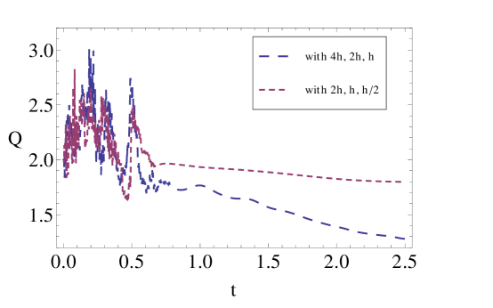
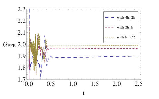
Figs. 3 and 4 show $L^{2}$-norms of (84) and (85) respectively, obtained from evolving the particular initial data described above. We used 4 different resolutions to help see the trends in the respective $Q$’s. At early times, the solution is not yet in the asymptotic scaling regime for the convergence factors, however that they are typically greater than $2$ indicates that the solution error is nevertheless small. Also, the trends going to higher resolution, in particular at later times, appear consistent with second-order convergence.

The early-time deviations in Fig. 4 coincide with an initial transient associated with the gauge transition described by (80), that emanates from the boundary and dissipates as it travels further into the interior. This transient is clearly seen as a temporary dip in the point-wise convergence factors for independent residuals near the boundary; taking the $L^{2}$-norm as was done in Fig. 4 to some extent masks this dip, though is still visible with the highest resolution curve in that plot. Nevertheless, this transient converges away in the sense that the region of the domain affected shrinks as resolution is increased.

VI Results

We now describe several early results obtained with this code. First, in Sec. VI.1, we show solutions of the Hamiltonian constraint with a scalar field source (III.2), demonstrating that this approach is capable of producing initial data containing trapped surfaces. Then, in Sec. VI.2 we show the evolution of initial data describing highly deformed black holes that subsequently shed their asymmetries via quasi-normal ringdown. A proper extraction of quasi-normal modes, and in particular a meaningful comparison with perturbative calculations where these modes can be defined, requires the identification of a reference background metric and a transformation of the solution to a gauge consistent with that of the perturbative calculations. We have made no attempt in this direction, besides matching the areal radius on the extraction sphere, and do in fact see what appear to be gauge modes. Nevertheless, we can extract the leading order linear quasi-normal modes, and for the higher angular number modes, use a simple forced harmonic oscillator model to identify what appear to be non-linearly excited harmonics of the lower angular modes. In Sec. VI.3 we discuss the extracted boundary stress energy tensor of these solutions, and in Sec. VI.4 analyse how well the CFT state can be described by hydrodynamics. We find that the extracted stress energy tensor is consistent, essentially to within numerical truncation error, with that of a viscous, conformal fluid from $t=0$ onwards. In Sec. VI.6, we transform these solutions onto a Minkowski piece of the boundary, and find an initial fluid geometry that resembles a Lorentz-flattened pancake. Defining the beam-line direction as the one along which the initial data is flattened, the evolution of this fluid exhibits both longitudinal and transverse flow relative to the beam-line, with most of the energy flowing along the longitudinal directions.

VI.1 Strong-field Solutions of the Hamiltonian Constraint

To generate black holes spacetimes, we choose initial data where the deviation from pure AdS₅ is sourced by a highly compact distribution of scalar field energy, with profile given by (37). In this paper we only consider free, massless scalar fields, so $V(\phi)=0$ in (35). In this section, we begin by focusing on spherically symmetric initial data, so $w_{x}=w_{y}=1$ in (37).

Fig. 5 summarizes solutions of the Hamiltonian constraint (III.2) by plotting the maximum value of the conformal factor versus the maximum of the scalar field (both maxima occur at the origin of the domain for these initial data). Let us begin by contrasting the qualitative behavior of this plot with its counterpart in the asymptotically flat case, presented in Pfeiffer and York (2005). This earlier work employed the conformal thin sandwich method to solve the constraints. There, it was discovered that there exists a critical point above which no numerical solutions for the initial data could be found, and where the conformal factor diverges as the amplitude approaches the critical point. Even more surprisingly, it was found that generalizing to the extended conformal thin sandwich method gives rise to a branch point instead of a critical point, with solutions along the upper branch exhibiting non-uniqueness for any given set of initial data.

Figure 5: Maximum conformal factor vs. maximum amplitude of initial scalar matter distribution, with Gaussian profile (35) with $A=\phi_{\text{max}}$, $\delta=0.2$ (with AdS scale $L=1$), $w_{x}=w_{y}=1$ and $R_{0}=0$. We differentiate between “strong-field” and “weak-field” data based on whether there is a trapped surface present on the initial slice or not, respectively. (Though of course this distinction is somewhat arbitrary, particularly since subsequent evolution of weak-field data could eventually result in black hole formation, as argued in Bizon and Rostworowski (2011) even for arbitrarily small amplitude initial data.) The value of $\phi_{max}$ beyond which trapped surfaces are found in the initial data is indicated by the dashed vertical line. The open circles denote numerical solutions, while the solid lines are fits to the data, as shown.

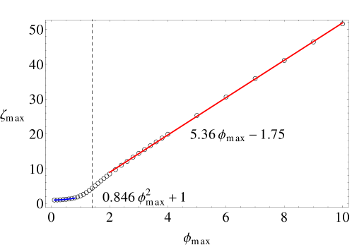
In contrast, we find no divergent behavior in the conformal factor, nor any behavior suggesting the non-uniqueness of solutions $\phi_{max}$, at least in the regime where the cosmological length scale is relevant. Furthermore, the linear dependence of the maximum of the conformal factor versus amplitude for large amplitude data suggests that the AdS₅ Hamiltonian constraint admits conformal solutions for arbitrarily strong initial matter distributions. Of course, given the presence of the cosmological constant and its relevance on these scales, it is not too surprising that we find such qualitatively different behavior compared to the asymptotically flat case. From a more formal perspective, the local existence and uniqueness of solutions to non-linear elliptic PDEs can be understood by applying a maximum principle, where the signs and relative magnitudes of coefficients in the PDE are crucial; one can show that in this regard cosmological the constant in AAdS spacetimes “helps”.

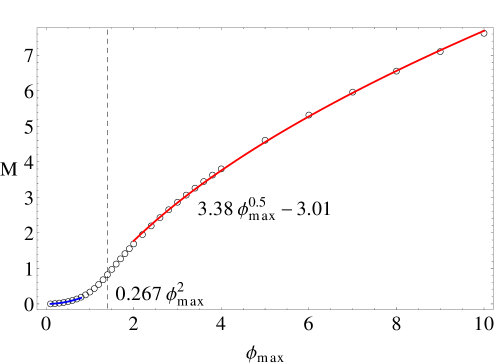
Fig. 6 shows a plot of the conserved mass $M$ of the spacetime versus scalar field amplitude, computed from the quasi-local stress tensor (21) as follows. We take a spatial $t={\rm const.}$ (here $t=0$) slice in $\partial M_{q}$, with induced 3-metric $\sigma_{\mu\nu}$, lapse $N$ and shift $N^{i}$ such that $\Sigma_{\mu\nu}dx^{\mu}dx^{\nu}=-N^{2}dt^{2}+\sigma_{ij}(dx^{i}+N^{i}dt)(dx^{j}+N^{j}dt)$, then compute

$$M=\underset{q\rightarrow 0}{\lim}\int_{\Sigma}d^{3}x\sqrt{\sigma}N({}^{(q)}T_{\mu\nu}u^{\mu}u^{\nu})$$ (86)

where $u^{\mu}$ is the time-like unit vector normal to $t={\rm const.}$ Note that for a vacuum AdS-Schwarzschild black hole, this prescription gives a result consistent with the usual definition of its mass from the analytic solution, namely $M=3\pi\left({r_{0}}^{2}/8\right)$, where $r_{0}=r_{H}\sqrt{1+r_{H}^{2}/L^{2}}$, given a horizon with areal radius $r_{H}$.

Figure 6: AdS mass vs. maximum amplitude of massless scalar matter, with Gaussian profile defined by $A=\phi_{\text{max}}$, $(x_{0},y_{0})=(0,0)$, $\delta=0.2$. Conventions are the same as those used in Fig. 5. In cases where trapped surfaces are present (to the right of the dashed vertical line), an estimate of the mass based on the area of the apparent horizon gives a value very close the asymptotic mass plotted here, though systematically smaller (the two values would essentially be indistinguishable on the scale of this figure, hence we only show the asymptotic mass to avoid clutter).

VI.2 Quasinormal Ringing

As a first application of our evolution scheme, we study the quasi-normal ringdown of an initially high distorted (i.e. non-spherical) black hole. Here we focus on the dynamics of the bulk, and in the following sections discuss the corresponding dynamics of the CFT boundary stress tensor. For some previous work on the subject see for example Horowitz and Hubeny (2000); Cardoso et al. (2003); Kovtun and Starinets (2005); Janik and Peschanski (2006); Teaney (2006); Friess et al. (2007). For a review of black hole quasi-normal modes in AdS see Berti et al. (2009). Again, we use large-amplitude scalar field data to create an initial slice of the spacetime containing a trapped surface, and here introduce a non-trivial $\chi$-dependence by adjusting the shape of the profile through the parameters $w_{x}$ and $w_{y}$ as defined in (37). Specifically, unless otherwise stated we choose $R_{0}=0.0$, $\delta=0.2$, $w_{x}=4.0$, $w_{y}=16.0$, and vary the amplitude $A_{0}$ to control the size of the resultant black hole.

First, to demonstrate that we are looking at relatively large perturbations of the spherical black hole, in Fig. 7 we plot the ratio of the equatorial $c_{eq}$ to polar $c_{p}$ proper circumferences of the apparent horizon versus time. A geometric sphere has $c_{eq}/c_{p}=1$, whereas a geometric disk $c_{eq}/c_{p}=\pi/2$. The $w_{y}/w_{x}=4$ case studied in detail here has $c_{eq}/c_{p}(t=0)\approx 1.2$, so a fairly sizeable deformation. For certain quasi-normal mode and hydrodynamic extraction results we also show data from the $w_{y}/w_{x}=32$ case, which has a very large initial $c_{eq}/c_{p}(t=0)\approx 2.2$.

Figure 7: The ratio $c_{eq}/c_{p}$ of proper equatorial to polar circumference of the apparent horizon versus time. $w_{y}/w_{x}$ denotes parameters in the initial data describing the scalar field profile (37), and $w_{y}/w_{x}=4$ is the canonical case studied in this paper, though for interest we also show examples representing a weaker and stronger initial asymmetry. In all cases, the final black hole has radius $r_{h}\approx 5$. Note that a geometric sphere has $c_{eq}/c_{p}=1$, whereas a geometric disk has $c_{eq}/c_{p}=\pi/2$. Thus, even the $w_{y}/w_{x}=4$ case is initially a rather large deformation of the $3$-sphere; the curve for the more extreme case $w_{y}/w_{x}=32$ implies that at early times the Gaussian curvature is negative over at least some regions of the horizon.

To extract the quasi-normal modes, the first step would be to transform our metric to a gauge consistent with standard perturbative calculations for quasi-normal modes. This is a rather non-trivial step in general, and we do not do so here, hoping that our asymptotic gauge choice is sufficiently close to that of the perturbative calculations that artifacts introduced are small. As we shall see, this seems to hold to good approximation, though we do find modes that appear to be pure gauge.

We begin by projecting our field variables onto the spherical harmonics on $S^{3}$; see Avery (2000). We first need the standard spherical harmonics on $S^{2}$:

$$Y_{lm}(\theta,\phi)=\sqrt{\frac{2l+1}{4\pi}\frac{(l-m)!}{(l+m)!}}P^{m}_{l}(\cos\theta)\exp(im\phi)$$ (87)

where the associated Legendre polynomials are defined as:

$$P^{m}_{l}(x)=\frac{(-1)^{m}}{2^{l}l!}\frac{d^{(l+m)}}{dx^{(l+m)}}(x^{2}-1)^{l}.$$ (88)

The scalar spherical harmonics on $S^{3}$ are then:

$$\mathbb{S}(klm) = (-1)^{k}i^{l}(2l)!!\sqrt{\frac{2(k+1)(k-l)}{\pi(k+l+1)!}}$$ (89)

$$\times C^{l+1}_{k-l}(\cos\chi)\sin^{l}(\chi)Y_{lm}(\theta,\phi)$$

where the Gegenbauer polynomials are defined as:

$$C^{a}_{k}(x) = \frac{(-2)^{k}}{k!}\frac{\Gamma(k+a)\Gamma(k+2a)}{\Gamma(a)\Gamma(2k+2a)}(1-x^{2})^{-a+1/2}$$ (90)

$$\times\frac{d^{k}}{dx^{k}}(1-x^{2})^{k+a-1/2}.$$

Our restriction to solutions that preserve a symmetry in $\theta,\phi$ mandates that we have $l=0,m=0$.

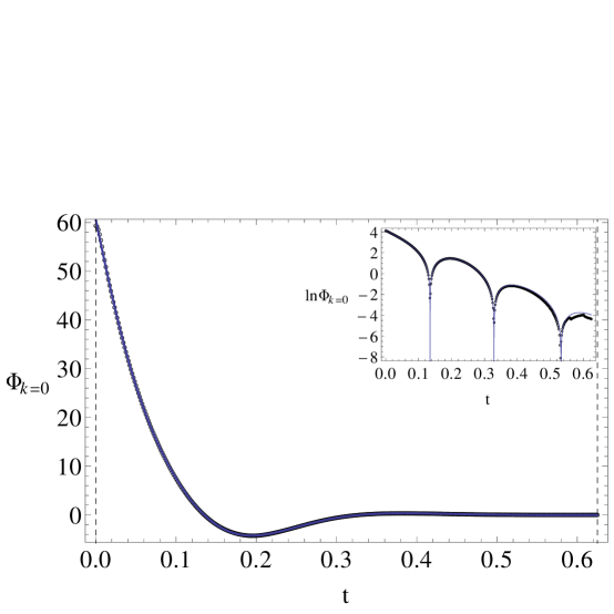
For perturbations of the scalar field, these $\mathbb{S}(klm)$ scalar harmonics exist for all $k\geq 0$. Fig. 8 shows the scalar field projected onto the 3-sphere ($k=0$), for a simulation with initial $w_{y}/w_{x}=4$ and whose final state black hole has horizon radius $r_{h}=5$. The quasi-normal mode frequencies extracted from the scalar field are collected in Appendix C, under Table 4 for the $n=0$ fundamental mode and under Table 5 for the $n=1$ first overtone. This was done for several $r_{h}$ cases, wherein each pair of fundamental and first overtone was found by a simultaneous non-linear least-squares fit to two damped sinusoids, one corresponding to the $n=0$ fundamental and the other corresponding to the $n=1$ overtone. Each sinusoid is described by four parameters. The $n=0$ fundamental frequencies $\omega_{r}$ and $\omega_{i}$ scale linearly with $r_{h}$, and their dependence on $k$ shows that $\omega_{r}$ increases with $k$ and that $\omega_{i}$ decreases with $k$. The $n=1$ first overtone frequencies $\omega_{r}$ and $\omega_{i}$ also scale linearly with $r_{h}$, as with the $n=0$ frequencies; however, the dependence on $k$ differs from the $n=0$ fundamental case in that the $\omega_{r}$ and $\omega_{i}$ both increase with $k$. To make contact with earlier work on quasi-normal modes in AdS, we note that the frequencies extracted for the $n=0$ fundamental are a close match to those found in the seminal study Horowitz and Hubeny (2000) on this subject.

Figure 8: The leading-order behavior of the scalar field variable $\bar{\phi}$ near the boundary $q=1$, projected onto the $3$-sphere by $\Phi_{k=0}=\int d\Omega_{3}(\bar{\phi}/q)\mathbb{S}(000)$, and plotted over a global time interval of $t\in[0,0.62]$ (open circles). A fit (solid line) $\Phi_{k=0}^{fit}$ is extracted using the data inbetween the dashed vertical lines. The inset shows a logarithmic plot of the data and the fit over the full global time interval.

Figure 9: The leading-order behavior of the metric variable $\bar{g}_{\chi\chi}$ near the boundary $q=0$, projected onto the $\mathbb{S}(200)$ scalar harmonic by $(\mathcal{G}_{\chi\chi})_{k=2}=\int d\Omega_{3}(\bar{g}_{\chi\chi}/q)\mathbb{S}(200)$, plotted over a global time interval of $t\in[0,8\pi]$ (open circles). A fit (solid line) $(\mathcal{G}_{\chi\chi})_{k=2}^{fit}$ is extracted using the data inbetween the dashed vertical lines. The inset shows a logarithmic plot of the data and the fit over the full global time interval. Other metric variables show similar behavior.

	fund.	k=2
	$\frac{r_{h}}{L}$=12.2	$(1.640\pm 0.007)-i(0.902\pm 0.067)\frac{L}{r_{h}}$
	$\frac{r_{h}}{L}$=11.3	$(1.640\pm 0.005)-i(0.895\pm 0.058)\frac{L}{r_{h}}$
	$\frac{r_{h}}{L}$=10.5	$(1.641\pm 0.002)-i(0.876\pm 0.039)\frac{L}{r_{h}}$
	$\frac{r_{h}}{L}$=9.0	$(1.643\pm 0.003)-i(0.864\pm 0.028)\frac{L}{r_{h}}$
	$\frac{r_{h}}{L}$=6.5	$(1.650\pm 0.0007)-i(0.841\pm 0.010)\frac{L}{r_{h}}$
	$\frac{r_{h}}{L}$=5.0	$(1.661\pm 0.0006)-i(0.837\pm 0.005)\frac{L}{r_{h}}$
	$\frac{r_{h}}{L}$=4.5	$(1.666\pm 0.0006)-i(0.823\pm 0.004)\frac{L}{r_{h}}$
	$\frac{r_{h}}{L}$=4.0	$(1.675\pm 0.0005)-i(0.823\pm 0.003)\frac{L}{r_{h}}$
	$\frac{r_{h}}{L}$=3.3	$(1.692\pm 0.0004)-i(0.808\pm 0.002)\frac{L}{r_{h}}$

Table 1: The fundamental ($n=0$) quasi-normal mode frequencies $\omega_{r}-i\omega_{i}$ extracted from the metric variable $\bar{g}_{\chi\chi}$. These are shown for various horizon radii $r_{h}$ of the final state AdS-Schwarzschild black hole and for $SO(4)$ quantum numbers $k=2,l=0,m=0$. Uncertainties are estimated from convergence studies.

	n=1	k=2
	$\frac{r_{h}}{L}$=12.2	$(3.497\pm 0.131)\frac{r_{h}}{L}-i(2.087\pm 0.142)\frac{r_{h}}{L}$
	$\frac{r_{h}}{L}$=11.3	$(3.320\pm 0.156)\frac{r_{h}}{L}-i(2.185\pm 0.174)\frac{r_{h}}{L}$
	$\frac{r_{h}}{L}$=10.5	$(3.378\pm 0.339)\frac{r_{h}}{L}-i(2.120\pm 0.368)\frac{r_{h}}{L}$
	$\frac{r_{h}}{L}$=9.0	$(3.256\pm 0.078)\frac{r_{h}}{L}-i(2.100\pm 0.125)\frac{r_{h}}{L}$
	$\frac{r_{h}}{L}$=6.5	$(3.329\pm 0.178)\frac{r_{h}}{L}-i(2.091\pm 0.091)\frac{r_{h}}{L}$
	$\frac{r_{h}}{L}$=5.0	$(3.103\pm 0.264)\frac{r_{h}}{L}-i(2.626\pm 0.495)\frac{r_{h}}{L}$
	$\frac{r_{h}}{L}$=4.5	$(3.217\pm 0.084)\frac{r_{h}}{L}-i(2.718\pm 0.130)\frac{r_{h}}{L}$
	$\frac{r_{h}}{L}$=4.0	$(3.274\pm 0.051)\frac{r_{h}}{L}-i(2.688\pm 0.070)\frac{r_{h}}{L}$
	$\frac{r_{h}}{L}$=3.3	$(3.318\pm 0.059)\frac{r_{h}}{L}-i(2.914\pm 0.307)\frac{r_{h}}{L}$

Table 2: The first overtone ($n=1$) quasi-normal mode frequencies $\omega_{r}-i\omega_{i}$ extracted from the metric variable $\bar{g}_{\chi\chi}$. These are shown for various horizon radii $r_{h}$ of the final state AdS-Schwarzschild black hole and for $SO(4)$ quantum numbers $k=2,l=0,m=0$. Uncertainties are estimated from convergence studies.

For the metric, the $\mathbb{S}(klm)$ scalar harmonics are restricted by $0\leq l\leq k$. The $k=1$ mode is not associated with any physical degrees of freedom Kodama and Ishibashi (2003), and these can be ignored; indeed our choice of initial data where the scalar field profile is symmetric about $\chi=\pi/2$ prevent these from being excited. The $k=0$ mode corresponds to a perturbation of a black hole that is itself spherically-symmetric in all the $S^{3}$ angles $\chi,\theta,\phi$. Thus, as a consequence of Birkhoff’s theorem, we might also expect to ignore this $k=0$ case as we have with $k=1$. However, despite this reasoning, we see non-trivial dynamics in the data’s projection onto the $k=0$ scalar harmonic. To understand why, recall that we have not transformed our metric to a gauge that is consistent with the standard one assumed by the perturbative calculations for quasi-normal modes. Consequently, the metric components that we extract generally contain both physical quasi-normal modes as well as contributions from gauge modes that are introduced by our “non-standard” choice of time-slicing, and of the $r$ and $\chi$ coordinates on each slice. This gauge contribution is of course present in the data for all $k$, and is most obvious in the $k=0$ projection since it contains no physical quasi-normal modes. For $k\geq 2$, this gauge contribution manifests itself as a decaying mode (i.e. a mode whose frequency has a negligibly small real part). In the following, we consider the $k\geq 2$ modes of the metric, taking into account this gauge contribution.

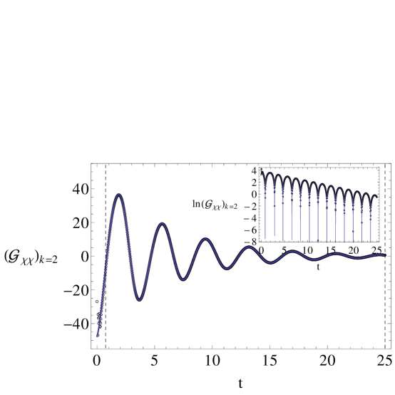
Fig. 9 shows a representative metric variable projected onto the $\mathbb{S}(200)$ ($k=2$) scalar harmonic, for a simulation with final state horizon radius $r_{h}=5$ and initial asymmetry $w_{y}/w_{x}=4$. The quasi-normal mode frequencies extracted from this representative metric variable are displayed in Table 1. This analysis was repeated for several simulations with varying $r_{h}$ but fixed $w_{y}/w_{x}=4$. Fits to damped sinusoids yield $n=0$ fundamental frequencies with imaginary parts $\omega_{i}$ that scale as $\sim 1/r_{h}$, and real parts $\omega_{r}$ that are largely insensitive to these changes in $r_{h}$.

Obtaining the $\mathbb{S}(200)$ harmonic’s $n=1$ overtone from the metric variables is more difficult, largely because it decays much more quickly than the $n=0$ fundamental. To obtain good fits, we focus on an early-time segment of the data, and substract the $n=0$ fit, then fit to the remainder. The quasi-normal frequencies extracted in this way are tabulated in Table 2. This table shows that the $n=1$ fundamental frequencies $\omega_{r}$ and $\omega_{i}$ both scale linearly with $r_{h}$. To compare with earlier work, notice that these extracted frequencies for the $n=1$ overtone are a close match to the first set of “fast-modes” found in Friess et al. (2007), and that the extracted frequencies for the $n=0$ fundamental closely match the low-lying “slow-modes” found in the same study.

Discrepancies with the linear quasi-normal mode description start to appear in the next highest scalar harmonic $\mathbb{S}(400)$ ($k=4$): direct fitting yields a dominant frequency that does not match Friess et al. (2007). The $k=4$ fundamental mode with frequency $\omega_{4}\approx 2.949+i3.428/r_{h}$ is present, but is overshadowed by a mode with frequency $\omega^{dbl}_{4}\approx 3.312+i1.627/r_{h}$, which is close to double that of the $k=2$ fundamental $\omega_{2}\approx 1.652+i0.826/r_{h}$ that appears in Table 1. We expect that this frequency-doubling in the $k=4$ modes arises from a non-linear mode-coupling, which we attempt to model as a damped harmonic oscillator driven at double the frequency of the $k=2$ fundamental mode. Given a $k=2$ fundamental mode $\Psi_{2}(t)=A_{2}\exp\left(-i\omega_{2}t\right)$, the $k=4$ mode $\Psi_{4}(t)$ in this simple model satisfies

$$\partial_{t}^{2}\Psi_{4}+k_{4}^{2}\Psi_{4}-\lambda_{4}\partial_{t}\Psi_{4}=B\exp\left(-2i\omega_{2}t\right),$$ (91)

$\lambda_{4}=\omega_{4i}$, $k_{4}^{2}=(\omega_{4r})^{2}+(\omega_{4i})^{2}$ (with the $r$ and $i$ subscripts denoting the real and imaginary components of the corresponding number respectively), and we expect the driving amplitude $B$ to scale as $B\sim{(A_{2})}^{2}$.

	$\frac{w_{y}}{w_{x}}$	$A_{4}$	$A^{dbl}_{4}$	$A^{g}_{4}$	$\omega^{g}_{4i}$	$\Delta\varphi$	$\frac{A^{dbl}_{4}}{(A_{2})^{2}}\times 10^{3}$
	$1.1$	$(1.49\pm 0.09)\times 10^{-3}$	$(6.44\pm 0.02)\times 10^{-3}$	$(4.40\pm 0.03)\times 10^{-4}$	$(1.23\pm 0.23)\frac{L}{r_{h}}$	$0.832\pm 0.011$	$4.03\pm 0.02$
	$4$	$2.75\pm 0.01$	$9.62\pm 0.01$	$0.508\pm 0.030$	$(1.26\pm 0.04)\frac{L}{r_{h}}$	$0.873\pm 0.032$	$4.00\pm 0.02$
	$32$	$(5.39\pm 0.04)\times 10^{1}$	$(1.16\pm 0.01)\times 10^{2}$	$1.59\pm 0.06$	$(1.16\pm 0.01)\frac{L}{r_{h}}$	$0.894\pm 0.066$	$4.60\pm 0.02$

Table 3: Extracted parameters from the $k=4$ fit corresponding to Fig. 10 at $w_{y}/w_{x}=4$, as well as for the largest and smallest $w_{y}/w_{x}$ cases considered. The fit includes the fundamental $k=4$ mode with amplitude $A_{4}$, a mode of amplitude $A^{dbl}_{4}$ that has twice the frequency of the $k=2$ fundamental mode of amplitude $A_{2}$, and a putative gauge mode $A^{g}_{4}\exp(-\omega^{g}_{4i}t)$. The model for the mode coupling discussed in the text predicts a phase difference between the frequency-doubled $k=4$ mode and its $k=2$ fundamental mode source of $\Delta\varphi\sim 0.842$, and that $A^{dbl}_{4}$ scales as the square $A_{2}$; these two quantities are shown in the last two columns of the table, and indicate the solution is reasonably consistent with the model. Uncertainties are estimated via convergence.

The solution of (91) is a sum of the $k=4$ fundamental mode and the driven mode

$$\Psi_{4}(t)=A_{4}\exp\left(-i\omega_{4}t\right)+A^{dbl}_{4}\exp\left(-2i\omega_{2}t\right),$$ (92)

where $A_{4}$ is a constant depending on the initial data, and $A^{dbl}_{4}$ is a (complex) constant depending upon the other parameters of the model via

$$A^{dbl}_{4}=(\tilde{\omega}_{r}+i\tilde{\omega}_{i})^{-1}B,$$ (93)

where we have introduced for notational convenience $\tilde{\omega}_{i}=4\omega_{2r}(2\omega_{2i}-\omega_{4i})$ and $\tilde{\omega}_{r}=(\omega_{4r})^{2}+(\omega_{4i})^{2}-4\left((\omega_{2r})^{2}-(\omega_{2i})^{2}+\omega_{4i}\omega_{2i}\right)$.

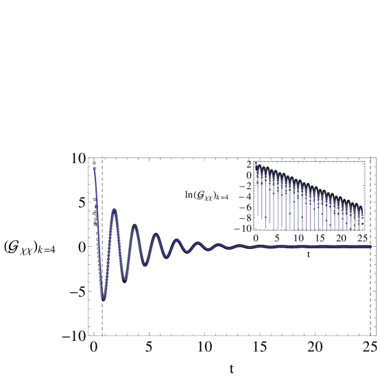
Our strategy is to compare the predictions of this simplified model of non-linear mode-mixing to the parameters extracted from the fits. In particular (93) gives us quantitative predictions for the relative amplitude and phase difference between the frequency-doubled $k=4$ mode and the $k=2$ fundamental mode that sources it: that the phase difference should be $\Delta\varphi=\arctan(\tilde{\omega}_{i}/\tilde{\omega}_{r})$, and that $A^{dbl}_{4}$ should scale as $({A_{2}})^{2}$. To test these predictions, we fit the $k=4$ data to two damped sinusoids simultaneously (in addition to the decaying gauge mode), though fixing their frequencies to $\omega_{4}$ and $2\omega_{2}$. We can then check if the extracted amplitude and phase of the frequency doubled mode matches the model prediction. The results, presented in Table 3 for three values of $w_{y}/w_{x}$, and an example fit is shown in Fig. 10 for the $w_{y}/w_{x}=4$ case, show good agreement with the model.

Figure 10: The leading-order behavior of the metric variable $\bar{g}_{\chi\chi}$ near the boundary $q=0$, projected onto the $\mathbb{S}(400)$ scalar harmonic by $(\mathcal{G}_{\chi\chi})_{k=4}=\int d\Omega_{3}(\bar{g}_{\chi\chi}/q)\mathbb{S}(400)$, plotted over a global time interval of $t\in[0,8\pi]$ (open circles). A fit (solid line) $(\mathcal{G}_{\chi\chi})_{k=4}^{fit}$ is extracted using the data inbetween the dashed vertical lines. This is a fit to a gauge mode, and two damped sinusoids with fixed frequencies $\omega_{4}\approx 2.949+i3.428/r_{h}$ and $2\ \omega_{2}\approx 2\times(1.652+i0.826/r_{h})$ (see Table  3 for the corresponding parameters of the fit). The inset shows a logarithmic plot of the data and the fit over the full global time interval. Other metric variables show similar behavior.

Figure 11: The normalized residuals for the $k=2$ and $k=4$ fits, corresponding to Fig. 9 and Fig. 10, respectively, where $(\mathcal{R}_{\chi\chi})_{k}=\left((\mathcal{G}_{\chi\chi})_{k}-(\mathcal{G}_{\chi\chi})_{k}^{fit}\right)/\left|(\mathcal{G}_{\chi\chi})_{k}^{fit})\right|$. This quantity shows the extent to which the projection of the metric element $\bar{g}_{\chi\chi}$ onto the $\mathbb{S}(k00)$ harmonic fails to be described by the sum of the $k$ quasi-normal mode, gauge mode, and for the $k=4$ case the non-linear mode. At times before $t\approx 1$, the residual becomes large going to smaller $t$ due to a growing phase offset between the data and the fit (see Fig. 9 for the $k=2$ case, and Fig. 10 for the $k=4$ case), and at very early times there is an additional contribution from the early-time transient. At late times there is a slight increase in the residual. This is largely a consequence of the fitting procedure and that we are plotting a normalized residual : the fit is dominated by the data at early times as the perturbation is decaying exponentially, hence a small phase difference between the fit and data will result in a normalized residual that grows with time.

Figure 12: The normalized difference $(\mathcal{P}_{\chi\chi})_{k_{max}}=\left(\int d\Omega_{3}(\bar{g}_{\chi\chi}/q)^{2}-\sum_{k=0}^{k=k_{max}}(\mathcal{G}_{\chi\chi})_{k}^{2}\right)/\left|\int d\Omega_{3}(\bar{g}_{\chi\chi}/q)^{2}\right|$. For the $w_{y}/w_{x}=4$ case, the contribution due to the $k>2$ ($k>4$) modes constitutes $\approx\%2$ ($\%0.1$) of the metric perturbation, and decreases with time (the metric modes decay faster with higher $k$).

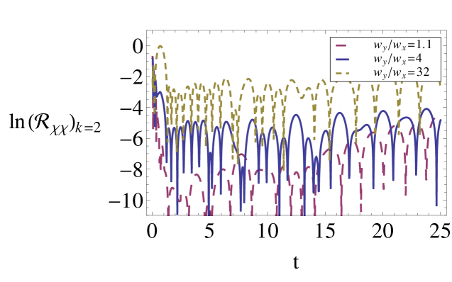
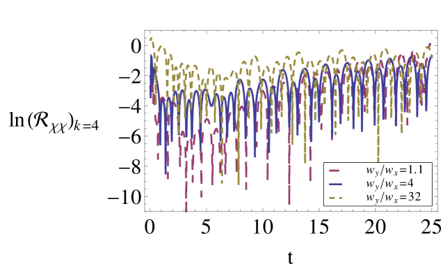
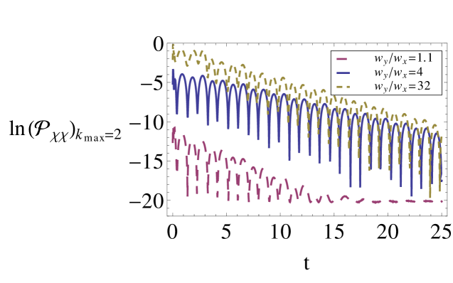
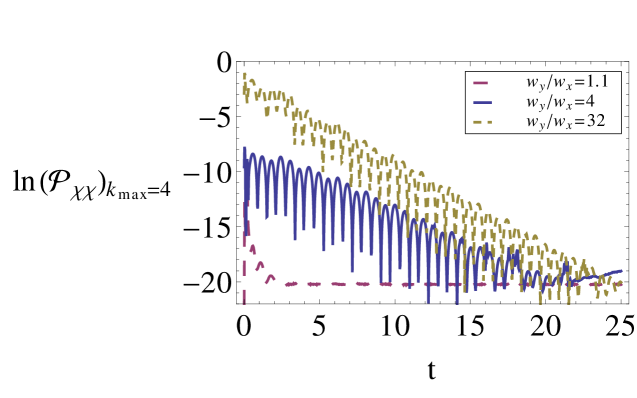
To quantify precisely how well the fits describe the actual data, we compute a residual that measures the difference between the data and the fits. This residual quantifies the part of the dynamics that we have not been able to fit to with linear quasi-normal modes supplemented by the pure decay gauge mode, and in the $k=4$ case, the mode arising from non-linear mode-mixing modeled by (91). The solid blue curve of the first panel of Fig. 11 depicts a normalized residual that is generated from the fit shown in Fig. 9. To illustrate the dependence on $w_{y}/w_{x}$, this analysis is repeated for the largest and smallest $w_{y}/w_{x}$ we have considered. The solid blue curve shows that the fit to the $k=2$ fundamental quasi-normal mode for $t\gtrsim 1$ captures all but $\approx 1\%$ of the perturbation projected onto the $\mathbb{S}(200)$ harmonic, for the $w_{y}/w_{x}=4$ case. The other curves show that a similar fit does worse for larger $w_{y}/w_{x}$, which is consistent with the expectation that other unmodeled effects (i.e. those not accounted for by the linear quasi-normal modes and our simplified model of the gauge and non-linear effects) should become more significant for data with larger deformations. Similarly, the solid blue curve of the second panel in Fig. 11 depicts the normalized residual corresponding to the fit shown in Fig. 10. It shows that for $t\gtrsim 1$, the fit to the fixed-frequency $k=4$ fundamental mode, the frequency-doubled $k=2$ mode and single gauge mode captures all but $\approx 5\%$ of the solution projected onto the $\mathbb{S}(400)$ harmonic for $w_{y}/w_{x}=4$. Again, the corresponding residual grows with larger initial asymmetry.

Finally, to quantify how much of the full solution is not accounted for by the $\mathbb{S}(200)$ and $\mathbb{S}(400)$ harmonics that we discussed above, we look at the normalized difference between the square of the full solution integrated over the 3-sphere, and the sum of the squares of all projections onto the $\mathbb{S}(k00)$ harmonics for all $k\leq k_{max}$. The result of this procedure is summarized in Fig. 12.

VI.3 Boundary Stress Tensor

In terms of the regularized metric variables (IV.2), and setting $L=1$, the stress energy tensor of the boundary CFT (19) evaluates to

$$\left<T_{tt}\right>_{\text{CFT}} = \frac{1}{64\pi}(-24\bar{g}_{\rho\rho,\rho}-32\bar{g}_{\chi\chi,\rho}-64\bar{g}_{\psi,\rho})$$

$$\left<T_{t\chi}\right>_{\text{CFT}} = \frac{1}{2\pi}(-\bar{g}_{t\chi,\rho})$$

$$\left<T_{\chi\chi}\right>_{\text{CFT}} = \frac{1}{64\pi}(-32\bar{g}_{tt,\rho}+24\bar{g}_{\rho\rho,\rho}+64\bar{g}_{\psi,\rho})$$

$$\left<T_{\theta\theta}\right>_{\text{CFT}} = \frac{\sin^{2}\chi}{64\pi}(-32\bar{g}_{tt,\rho}+24\bar{g}_{\rho\rho,\rho}+32\bar{g}_{\chi\chi,\rho}$$

$$+32\bar{g}_{\psi,\rho}).$$

and $\left<T_{\phi\phi}\right>_{\text{CFT}}=\sin^{2}\theta\left<T_{\theta\theta}\right>_{\text{CFT}}$. In the remainder of this section we discuss the CFT stress tensor extracted from a representative numerical solution, namely the $r_{h}=5$ quasi-normal ringdown spacetime described in the previous section.

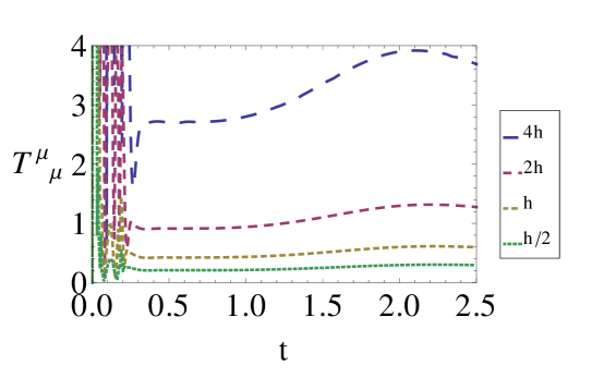
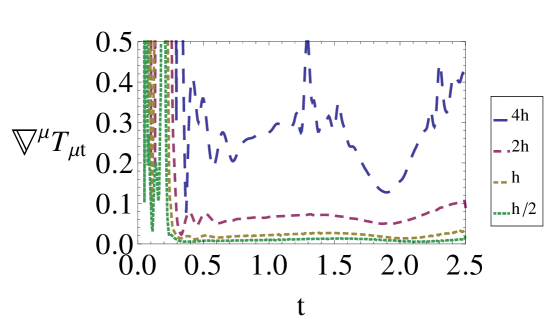
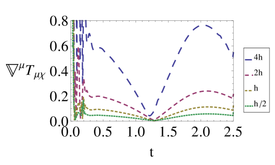
First, for a consistency check of expressions (VI.3), we test whether (to within truncation error) the stress tensor is traceless and whether it is conserved with respect to the Levi-Civita connection on the $\mathbb{R}\times S^{3}$ boundary. Results for the trace and two non-trivial components of the divergence are displayed in Fig. 13 and 14, respectively. These plots demonstrate that as resolution is increased, we are indeed converging to a CFT stress tensor that is conserved and traceless, i.e. to matter that obeys the hydrodynamic equations of motion, and whose equation of state is consistent with conformal invariance. Note that the early-time transient related to the initial gauge dynamics discussed in Sec. V.3 is also visible in these plots, though as with the independent residual it also converges away in the sense that it occupies a smaller region of the spacetime domain with increased resolution.

Figure 13: The trace $\left<{T^{\mu}}_{\mu}\right>_{\text{CFT}}$ of the boundary stress tensor, constructed from a simulation run at 4 different resolutions, labeled by the mesh spacing relative to the highest resolution run $h$. Here the $L^{2}$-norm of $\left<{T^{\mu}}_{\mu}\right>_{\text{CFT}}$ is taken over the entire grid, and the trends indicate convergence to a trace-free stress tensor with increasing resolution.

Figure 14: Two components of the divergence of the stress tensor, $\nabla^{\mu}\left<T_{\mu t}\right>_{\text{CFT}}$ (top) and $\nabla^{\mu}\left<T_{\mu\chi}\right>_{\text{CFT}}$ (bottom), constructed from a simulation run at 4 different resolutions, labeled by the mesh spacing relative to the highest resolution run $h/2$. The $L^{2}$-norm of the respective components are taken over the entire grid, and the trends indicate convergence to a conserved stress tensor with increasing resolution.

Figure 15: The energy density $\left<T_{tt}\right>_{\text{CFT}}$ of the boundary CFT, displayed on a ($t,\chi$) spacetime diagram, extracted from the $r_{h}=5$ quasi-normal black hole ringdown simulation described in Sec. VI.2. The first panel corresponds to the $w_{y}/w_{x}=4$ case, and the $w_{y}/w_{x}=32$ case in the second panel is included for comparison.

Figure 16: The $S^{2}$ component $\left<T_{\theta\theta}\right>_{\text{CFT}}$ of the boundary CFT stress tensor, displayed on a ($t,\chi$) spacetime diagram, extracted from the $r_{h}=5$ quasi-normal black hole ringdown simulation described in Sec. VI.2. The first panel corresponds to the $w_{y}/w_{x}=4$ case, and the $w_{y}/w_{x}=32$ case in the second panel is included for comparison.

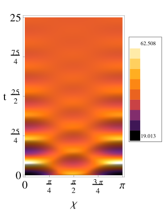
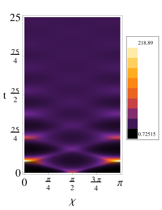
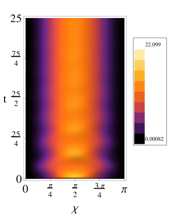
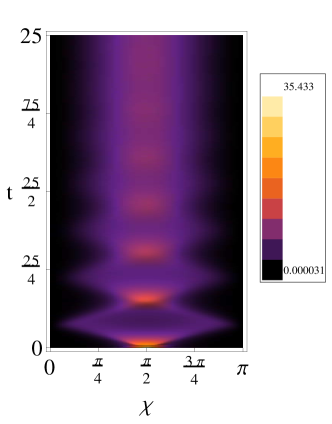
In Figs. 15 and 16 we display representative components of the boundary CFT stress tensor on $\mathbb{R}\times S^{3}$ spacetime diagrams, specifically the energy density $\left<T_{tt}\right>_{\text{CFT}}$ and $S^{2}$ component of the pressure $\left<T_{\theta\theta}\right>_{\text{CFT}}$ respectively. At $t=0$ the boundary state is clearly inhomogeneous, and in time evolves to a homogeneous state in a manner that mirrors the quasi-normal decay of the spacetime to a static black hole.

VI.4 Hydrodynamic Description of the Boundary CFT

Essentially all known physical systems at sufficiently high temperature, including those described by quantum field theories, exhibit hydrodynamic behavior once local thermodynamic equilibrium has been attained. In the gauge/gravity duality, stationary black holes are dual to equilibrium thermal states, and studies have shown that perturbations of the bulk spacetime manifest as hydrodynamic behavior in the boundary CFT. See Hubeny et al. (2011) for a recent review, and Emparan (2011) for a review of the “blackfolds” approach, which is similar in spirit but connects the dynamics of a perturbed black brane with that of an enclosing world-volume via a derivative expansion of the Einstein field equations. Here, we have studied the evolution of initially highly distorted black holes, far from the perturbative regime, and so the question naturally arises: at what time does hydrodynamics become a good description of the boundary state? More precisely, we would like to know whether the extracted $\left<T_{\mu\nu}\right>_{\text{CFT}}$ on the $\mathbb{R}\times S^{3}$ boundary is that of the particular kind of fluid predicted by the duality, namely an $\mathcal{N}=4$ SYM fluid with equation of state $\epsilon=3P$ (where $\epsilon$ and $P$ are the energy density and isotropic pressure in the rest frame of the fluid, respectively), and transport coefficients that match those found via holographic methods Loganayagam (2008).

In the previous section, we showed that convergence trends in the solution imply that in the continuum limit, $\left<T_{\mu\nu}\right>_{\text{CFT}}$ is conserved and traceless. Thus, two necessary ingredients are already satisfied: conservation is required for the effective hydrodynamic variables to satisfy the Navier-Stokes equations, and for an isotropic fluid, tracelessness implies $\epsilon=3P$. In this section we show that one can map $\left<T_{\mu\nu}\right>_{\text{CFT}}$ to a corresponding set of hydrodynamic variables, and that essentially from the initial time, their behavior is consistent with that of an $\mathcal{N}=4$ SYM fluid, at least to within truncation error.

In a low-energy effective description, the hydrodynamic stress tensor can be expressed as a velocity-gradient expansion, i.e. as a power series in the covariant gradients of a local fluid $4$-velocity one form $u_{\nu}$:

$$T_{\mu\nu}=(\epsilon+P)u_{\mu}u_{\nu}+Pg_{\mu\nu}-2\eta\sigma_{\mu\nu}+\Pi_{\mu\nu},$$ (95)

where we have introduced the (symmetric, traceless) shear tensor

$$\sigma^{\mu\nu}=\perp^{\mu\alpha}\perp^{\nu\beta}\nabla_{(\alpha}u_{\beta)}-\frac{1}{d-1}\nabla_{\alpha}u^{\alpha}\perp^{\mu\nu},$$ (96)

and subsumed all higher-order terms under $\Pi_{\mu\nu}$. All covariant differentiation is performed with respect to the boundary metric $g_{\mu\nu}dx^{\mu}dx^{\nu}=-dt^{2}+d\chi^{2}+\sin^{2}\chi(d\theta^{2}+\sin^{2}\theta d\phi^{2})$, and $\perp^{\mu\nu}$ in (96) is the projector onto the spatial slices orthogonal to the fluid $4$-velocity

$$\perp^{\mu\nu}=g^{\mu\nu}+u^{\mu}u^{\nu}.$$ (97)

In this sub-section, we will for now ignore the higher-order terms, i.e. we set $\Pi_{\mu\nu}=0$. In terms of mapping from stress tensor to hydrodynamic variables this should be a good approximation except in situations where the shear $\sigma_{\mu\nu}$ of the flow becomes small, which does occur periodically during the evolution of the distorted black holes discussed here. These higher order terms would lead to additional problems regarding the uniqueness of the mapping that we will now attempt. In the sub-section following this one, we will employ a different strategy and will instead extract a minimal subset, then, assuming an $\mathcal{N}=4$ SYM fluid, test for consistency with higher order transport coefficients (instead of trying to directly measure all these quantities, as we will now proceed to do).

Let us first identify a set of independent fluid variables which we can use to characterize the stress tensor. This set certainly includes $\epsilon$ and $P$, the energy density and isotropic pressure in the rest frame of the fluid, respectively. Given the $SO(3)$ symmetry of our solutions, the (unit) 4-velocity vector must take the form $u^{\mu}=\gamma(1,v,0,0)$ in $(t,\chi,\theta,\phi)$ coordinates, with $\gamma=1/\sqrt{1-v^{2}}$. This gives us a third fluid variable to add to our list: $v$, the $\chi$-coordinate velocity of the flow. As for the shear $\sigma_{\mu\nu}$, notice that it is symmetric, traceless and satisfies the identity $u^{\mu}\sigma_{\mu\nu}=0$. Together with the imposed $SO(3)$ symmetry, these imply that $\sigma_{\mu\nu}$ only has one degree of freedom in $d=4$ dimensions. Thus defining $\sigma_{\chi\chi}=\sigma$, one can straightforwardly show that the only other non-zero components of $\sigma_{\mu\nu}$ are:

$$\sigma_{t\chi}=-v\sigma,\hskip 11.38092pt\sigma_{tt}=v^{2}\sigma,\hskip 11.38092pt\sigma_{\theta\theta}=\frac{\sigma_{\phi\phi}}{\sin^{2}\theta}=-\frac{\sin^{2}\chi}{2\gamma^{2}}\sigma.$$ (98)

Given how $\eta$ and $\sigma$ always appear as a product in (95), we treat the two as a single quantity $\eta\sigma$ for the purposes of extraction. Thus, ignoring the higher-order terms $\Pi_{\mu\nu}$, the variables $(\epsilon,P,v,\eta\sigma)$, each of which is a function of $(t,\chi)$ in general, completely describes a conformal fluid flow on $\mathbb{R}\times S^{3}$ that preserves our $SO(3)$ symmetry.

On the gravity side, the quantities we measure are the components of the boundary stress tensor, which we denote $T_{\mu\nu}\equiv\left<T_{\mu\nu}\right>_{\text{CFT}}$ henceforth for the sake of brevity. In $SO(3)$ symmetry, there are $5$ non-zero stress tensor components, $4$ of which are independent. We can relate these $4$ to the fluid variables via (95):

$$T_{tt} = (\epsilon+P)\frac{1}{1-v^{2}}-P-2\eta\sigma v^{2}$$

$$T_{t\chi} = -(\epsilon+P)\frac{v}{1-v^{2}}+2\eta\sigma v$$

$$T_{\chi\chi} = (\epsilon+P)\frac{v^{2}}{1-v^{2}}+P-2\eta\sigma$$

$$T_{\theta\theta} = \sin^{2}\chi\left(P+\eta\sigma(1-v^{2})\right)$$ (99)

where $T_{\phi\phi}=\sin^{2}\theta T_{\theta\theta}$. Inverting these relations in favor of the rest-frame hydrodynamic quantities $(\epsilon,P,v,\eta\sigma)$, and defining the auxiliary quantities

$$\Xi \equiv \sqrt{(T_{\chi\chi}+2T_{t\chi}+T_{tt})(T_{\chi\chi}-2T_{t\chi}+T_{tt})}$$

$$T_{\psi} \equiv \frac{T_{\theta\theta}}{\sin^{2}\chi},$$ (100)

we obtain

$$\epsilon = \frac{1}{2}\left(T_{tt}-T_{\chi\chi}+\Xi\right)$$

$$P = \frac{1}{6}\left(\Xi+T_{\chi\chi}+4T_{\psi}-T_{tt}\right)$$

$$v = \frac{\Xi-T_{\chi\chi}-T_{tt}}{2T_{t\chi}}$$

$$\eta\sigma = \left[-T_{\chi\chi}^{3}+T_{\chi\chi}^{2}\left(-\Xi+T_{\psi}-2T_{tt}\right)\right.$$

$$+T_{\chi\chi}\left(T_{\psi}\left(\Xi+2T_{tt}\right)\right.\left.-T_{tt}\left(\Xi+T_{tt}\right)-4T_{t\chi}^{2}\right)$$

$$+T_{\psi}\left(T_{tt}\left(\Xi+T_{tt}\right)+4T_{t\chi}^{2}\right)\left.-2T_{t\chi}^{2}\Xi\right]/\left[6\Xi\right],$$

By itself, (VI.4) is not profound: the stress-tensor has 4 independent components, and we have simply mapped them to a new set of variables ($\epsilon,P,v,\eta\sigma$). The crucial question though is whether these variables behave as those of a conformal fluid. The answer appears to be yes, even for these initially highly distorted black holes.

Figure 17: The velocity field $v$ of the fluid describing the boundary CFT, displayed on a $t,\chi$ spacetime diagram, extracted from the $r_{h}=5$ quasi-normal black hole ringdown simulation described in Sec. VI.2. The first panel corresponds to the $w_{y}/w_{x}=4$ case, and the $w_{y}/w_{x}=32$ case in the second panel is included for comparison.

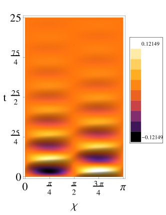
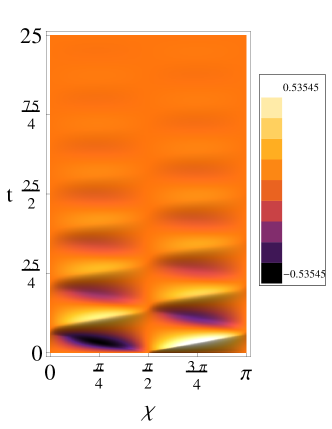
To support this claim, we first note that in all cases we have looked at to date, we are able to perform the inversion (VI.4) to obtain real-valued hydrodynamic variables that satisfy $\epsilon\geq 0$, $P\geq 0$ and $v\in(-1,1)$. Fig. 17 shows an example of $v(t,\chi)$, from the $r_{h}=5$ quasi-normal ringdown case discussed before. This suggests the stress tensor is consistent with that of some fluid. To check that it is a conformal fluid, in the top panel of Fig. 18 we show the quantity $(\epsilon-3P)/\epsilon$ resulting from the evolution at several different resolutions, using the same initial data (to contrast with Fig. 13, here we are not merely testing that the stress tensor is traceless, but rather the more restrictive property that it arises from fluid flow where in the rest frame of the flow the pressure is isotropic). At any given resolution, this quantity is certainly nonzero due to truncation error; however, except for a transient at the initial time, the trends show that it is converging to zero, at or better than first order. In other words, this says that after the initial transient, the boundary stress tensor behaves like a fluid with equation of state $\epsilon=3P$ to within numerical truncation error. Fig. 19 is a close-up of the early transient behavior seen in Fig. 18, and as before for the convergence of the solution discussed in Sec. V.3, it appears to be converging away in the sense that it affects a smaller region in time as resolution increases.

An alternative way to present this information is displayed in the bottom panels of Fig.’s 18 and  19. Here, assuming first order convergence of the extracted quantities, we take the finest resolution result as the continuum solution with an uncertainty (from truncation error) given by the magnitude of the difference between the finest and next-to-finest resolution results; this error is shown as the shaded region about the finest resolution curve. For subsequent time-series plots we will display the data in this format.

Figure 18: The quantity $(\epsilon-3P)/\epsilon$, which measures the extent to which the hydrodynamic description is that of a fluid with equation of state $\epsilon=3P$. The first panel is constructed from simulations run at 4 different resolutions, labeled by the mesh spacing relative to the highest resolution run $h/2$. What is shown at each time is the $L^{2}$-norm of $(\epsilon-3P)/\epsilon$ taken over the entire grid. Except possibly for an early transient (see Fig. 19), that this quantity is converging to zero shows that $\epsilon=3P$ to within truncation error. In the second panel we interpret the finest resolution data as the continuum solution to within an uncertainty (shaded region), obtained from the magnitude of the difference between the highest and next to highest resolution data (this assumes first order convergence of the extracted quantities).

Figure 19: An expanded view of Fig. 18 at early times.

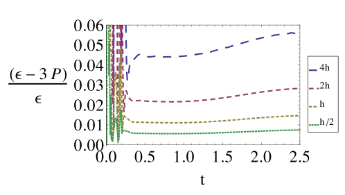
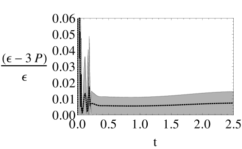
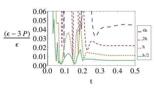
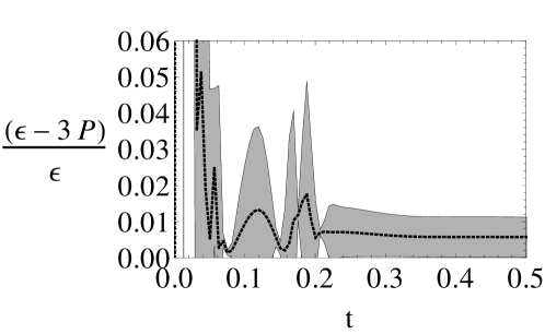
From this data we might also try to extract the lowest-order transport coefficient, namely the shear viscosity $\eta$, but here we encounter the two primary limitations of this sub-section’s extraction method. First, this method only allows us to extract the product $\eta\sigma$, so in order to find $\eta$ we must divide by an independent calculation of $\sigma$. Such a calculation may be achieved by substituting the extracted velocity field into (96), which yields $\sigma|_{v}$, so we can compute $\eta\sigma/\sigma|_{v}\approx\eta$. Given our time-symmetric initial data, this $\sigma|_{v}$ has zeros at $t=0$, and periodically after that. Even though the “true” $\eta\sigma$ necessarily has zeros at exactly the same times, the extracted $\eta\sigma$ will not, because we have ignored the $\Pi_{\mu\nu}$ higher-order contributions in the map. Thus, such a calculation of $\eta\sigma/\sigma|_{v}\approx\eta$ has the unattractive feature of diverging whenever $\sigma|_{v}=0$. Secondly, and more crucially, this method does not readily extend to allow the extraction of the higher-order transport coefficients. To remedy these shortcomings, we will now make use of a more general method to analyze the hydrodynamic behavior of the CFT $T_{\mu\nu}$.

VI.5 Higher-order Hydrodynamics

In this section, we present an alternative method for comparing $T_{\mu\nu}\equiv\left<T_{\mu\nu}\right>_{\text{CFT}}$ with the stress tensor of an $\mathcal{N}=4$ SYM fluid. To accomplish this, let us first add as many higher-order terms $\Pi_{\mu\nu}$ to the hydrodynamic stress tensor (95) as is presently known, which includes viscous corrections up to second-order in the gradient expansion. This gives four additional higher-order transport coefficients to supplement the shear viscosity $\eta$: the stress relaxation time $\tau_{\pi}$, the shear vorticity coupling $\tau_{\omega}$, the shear-shear coupling $\xi_{\sigma}$, and the Weyl curvature coupling $\xi_{C}$. Our strategy here will be different from the one described in the previous sub-section, where we had first extracted all hydrodynamic variables from the CFT stress tensor components, then exhibited evidence that the conformal constitutive relations hold. Instead, we will now assume that the conformal constitutive relations hold at the outset, allowing us to reconstruct the hydrodynamic stress tensor order by order using only the energy density $\epsilon$ and the fluid four-velocity $u^{\mu}$.

Figure 20: The mismatch $\Delta T^{i_{max}}_{\theta\theta}$ between the CFT stress tensor and the reconstructed hydrodynamic stress tensor with viscous corrections up to order $i_{max}=0,1,2$, for a simulation run with $w_{y}/w_{x}=4$ initial data, whose final state black hole has horizon radius $r_{h}=5$. Here, $\Delta T^{i_{max}}_{\theta\theta}\equiv T_{\theta\theta}-\sum_{i=0}^{i_{max}}T_{\theta\theta}^{(i)}$, and the plots are normalized by the fluid energy density $\epsilon$. As discuss in the text and Fig. 18, what is shown in each case is the data from the highest resolution run (dashed line) together with an estimated uncertainty (shaded region). Ideal hydrodynamics (top) shows a small residual mismatch; this is almost gone including first order viscous corrections (middle), and zero to within truncation error when second order corrections are added (bottom).

Figure 21: The same set of plots as described in Fig. 20, though here from the simulation of the $w_{y}/w_{x}=32$ initial data. Notice the larger relative mismatches at a given order of the expansion compared to the $w_{y}/w_{x}=4$ case in Fig. 20, and that there is still a small residual even after including all corrections through second order. The trend going from ideal (top) to second order viscous hydrodynamics (bottom) suggests that third and higher order corrections could further reduce the mismatch.

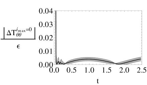
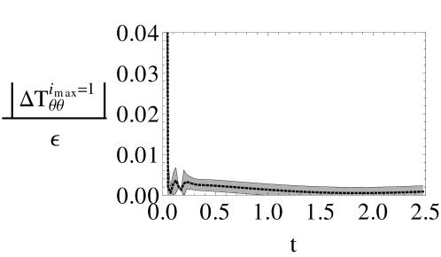
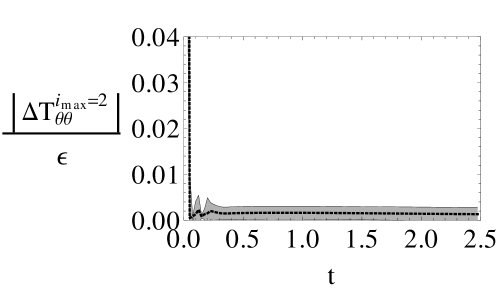
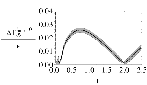
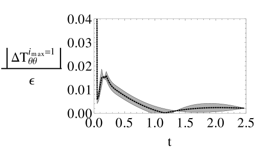
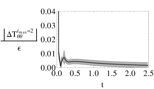
This reconstruction takes the form

$$T_{\mu\nu}=\sum_{i=0}^{\infty}T_{\mu\nu}^{(i)}$$ (102)

where $T_{\mu\nu}^{(0)}$ corresponds to the stress tensor of an ideal relativistic fluid, and $T_{\mu\nu}^{(i)}$ accounts for the $i^{th}$-order correction in a velocity-gradient expansion. These corrections are explicitly given in Loganayagam (2008) for an $\mathcal{N}=4$ SYM fluid:

$$T_{\mu\nu}^{(0)} = \epsilon u_{\mu}u_{\nu}+P\perp_{\mu\nu}$$

$$T_{\mu\nu}^{(1)} = -2\eta\sigma_{\mu\nu}$$

$$T_{\mu\nu}^{(2)} = -2\eta\left[-\tau_{\pi}u^{\lambda}\mathcal{D}_{\lambda}\sigma_{\mu\nu}+\tau_{\omega}\left({\omega_{\mu}}^{\lambda}\sigma_{\lambda\nu}+{\omega_{\nu}}^{\lambda}\sigma_{\lambda\mu}\right)\right]$$

$$+\xi_{\sigma}\left[{\sigma_{\mu}}^{\lambda}\sigma_{\lambda\nu}-\frac{\perp_{\mu\nu}}{3}\sigma^{\alpha\beta}\sigma_{\alpha\beta}\right]+\xi_{C}C_{\mu\alpha\nu\beta}u^{\alpha}u^{\beta}$$

where $C_{\mu\alpha\nu\beta}$ is the Weyl tensor and $\mathcal{D}$ is the Weyl covariant derivative defined in Loganayagam (2008). One further input are the constitutive relations for our $\mathcal{N}=4$ SYM fluid:

$$\epsilon = \frac{3{N_{c}}^{2}}{8\pi^{2}}\left(\pi T\right)^{4}=3P$$

$$\eta = \frac{{N_{c}}^{2}}{8\pi^{2}}\left(\pi T\right)^{3}$$

$$\tau_{\pi} = \frac{2-\ln 2}{2\pi T}$$

$$\tau_{\sigma} = \frac{\ln 2}{2\pi T}$$

$$\xi_{\sigma} = \xi_{C}=\frac{4\eta}{2\pi T}$$ (104)

where ${N_{c}}^{2}/(8\pi)=1/(16\pi G)$, and $T$ is the temperature of the fluid which we measure from the energy density $\epsilon$. The raw materials from which each $T_{\mu\nu}^{(i)}$ is built can be written in terms of CFT stress tensor components as

$$\epsilon = \frac{1}{2}\left(T_{tt}-T_{\chi\chi}+\Xi\right)$$

$$u^{\chi} = \frac{-2T_{t\chi}}{\sqrt{-4T_{t\chi}^{2}+\left(T_{tt}+T_{\chi\chi}+\Xi\right)^{2}}}$$ (105)

where $\Xi$ is defined by (VI.4).

We are now in the position to ask whether the boundary flow is consistent with an $\mathcal{N}=4$ SYM fluid, and if so, the extent to which higher-order corrections are important in describing it. We address these questions by comparing each of the reconstructed stress tensors $\sum_{i=0}^{i_{max}}T_{\mu\nu}^{(i)}$ for $i_{max}=0,1,2$ to the full boundary CFT stress tensor of the numerical solution. The results of this comparison are summarized in Figs. 20 and 21 for a representative stress tensor component (normalized by the energy density $\epsilon$). The plots in Fig. 20 are from the $w_{y}/w_{x}=4$ solution, where the maximum velocity in the flow reaches $\approx 0.12$ (see Fig. 17), and Fig. 21 is from the most asymmetric initial data case $w_{y}/w_{x}=32$ that exhibits a maximum velocity of $\approx 0.54$. For the former case, the solution converges to behavior that is different from ideal hydrodynamics by at most $\approx 0.5\%$ (modulo the transient near $t=0$); the inclusion of first-order and second-order corrections successively decrease this difference to a level which is essentially zero to within truncation error. The analogous plots for the larger asymmetry case in Fig. 21 show deviations from ideal hydrodynamics of up to $2.5\%$; adding first order corrections reduces the maximum deviation to $\approx 1.5\%$, and second-order corrections to just under $\approx 1\%$. This is a rather remarkable level of consistency, in particular considering the trends in Fig. 21 as succesively higher order viscous corrections are added.

VI.6 Passing to Minkowski Space

Thus far, in the field theory dual of deformed black holes, we have focused on fluid flows on the boundary of global AdS₅, namely $\mathbb{R}\times S^{3}$. As is clear from section VI.3, and in particular from the second panel of Fig. 15, the fluid flow is essentially a compressive wave which starts with its peak at the equator of $S^{3}$ and then travels to the poles and back, oscillating and damping out toward a static configuration where the temperature on $S^{3}$ is everywhere constant. In this section, we would like to make closer contact with real-world fluid flows by conformally mapping our extracted boundary solution on $\mathbb{R}\times S^{3}$ onto a corresponding flow in Minkowski space. To do this, we first explain the main concepts behind the conformal mapping; then we provide numerical results based on our most anisotropic deformed black hole solutions.

Up to a conformal transformation, $\mathbb{R}\times S^{3}$ is the covering space of Minkowski space, $\mathbb{R}^{3,1}$. Therefore, we can obtain fluid flows on $\mathbb{R}^{3,1}$ by restricting our results to an appropriate patch of $\mathbb{R}\times S^{3}$ and then conformally mapping to Minkowski space. There are many ways of doing this, simply because there are many ways of positioning the Minkowski space patch within $\mathbb{R}\times S^{3}$. We will mostly focus on one particular choice of patch which leads to a flow reminiscent of a head-on heavy ion collision—though, as on $\mathbb{R}\times S^{3}$, the initial conditions are characterized by full stopping rather than approximate rapidity independence. More specifically, the initial timeslice of our simulation, described as $t=0$ in $\mathbb{R}\times S^{3}$, will correspond to a Minkowski timeslice $t^{\prime}=0$ in which the fluid is stationary, and compressed into a region which is axisymmetric and significantly oblate. This is intended to be compared to the state of two heavy nuclei which have just achieved full overlap, though because the initial velocity profile is zero, a better analogy may be a quark-gluon plasma in a trap. The subsequent evolution of the fluid comprises two distinct types of expansion: longitudinal expansion along the axis of symmetry, and radial expansion. Overall, the flow preserves an $SO(3)$ subgroup of the conformal group $SO(4,2)$ (as it must since the black hole to which it is dual has an $SO(3)$ symmetry), but due to our choice of embedding of Minkowski space in $\mathbb{R}\times S^{3}$, this $SO(3)$ is not the obvious one composed of rotations around a point in a single timeslice. Rather, it is the conformal $SO(3)$ symmetry used in Gubser (2010b); Gubser and Yarom (2011); Staig and Shuryak (2011a, b) to study generalizations of Bjorken flow. Rotations around the axis of symmetry of the Minkowski space flow form an $SO(2)$ subgroup of the conformal $SO(3)$ symmetry. The rest of this $SO(3)$ is composed of special conformal transformations, corresponding to conformal Killing vectors of Minkowski space.

In order to map $\mathbb{R}\times S^{3}$, covered by global coordinates $x^{\mu}=(\tilde{t},\tilde{\chi},\tilde{\theta},\tilde{\phi})$, to $\mathbb{R}^{1,3}$, covered by coordinates $x^{a}=(t^{\prime},x_{1},x_{2},x_{3})$, we use the transformations

$$t^{\prime}/L = \frac{\sin\tilde{t}/L}{\cos\tilde{t}/L+\cos\tilde{\chi}}$$

$$x_{1}/L = \frac{\sin\tilde{\chi}}{\left(\cos\tilde{t}/L+\cos\tilde{\chi}\right)}\sin\tilde{\theta}\cos\tilde{\phi}$$

$$x_{2}/L = \frac{\sin\tilde{\chi}}{\left(\cos\tilde{t}/L+\cos\tilde{\chi}\right)}\sin\tilde{\theta}\sin\tilde{\phi}$$

$$x_{3}/L = \frac{\sin\tilde{\chi}}{\left(\cos\tilde{t}/L+\cos\tilde{\chi}\right)}\cos\tilde{\theta}\,.$$ (106)

The appearance of the AdS scale $L$ on the right hand side of (VI.6) is essential: only with this factor will (VI.6) lead to a conformal mapping of the metric

$$ds_{\mathbb{R}\times S^{3}}^{2} = g^{\mathbb{R}\times S^{3}}_{\mu\nu}dx^{\mu}dx^{\nu}$$ (107)

$$= -d\tilde{t}^{2}+L^{2}(d\tilde{\chi}^{2}+\sin^{2}\tilde{\chi}^{2}d\tilde{\theta}^{2}$$

$$\qquad{}+\sin^{2}\tilde{\chi}^{2}\sin^{2}\tilde{\theta}^{2}d\tilde{\phi}^{2})$$

to the standard Minkowski metric

$$ds_{\mathbb{R}^{3,1}}^{2}=g^{\mathbb{R}^{3,1}}_{ab}dx^{a}dx^{b}=-(dt^{\prime})^{2}+(dx_{1})^{2}+(dx_{2})^{2}+(dx_{3})^{2}\,.$$ (108)

The appearance of $L$ on the left hand side of (VI.6) is inessential: it could be replaced by any quantity with dimensions of length. Doing so would amount to altering Minkowski space by an uniform dilation of both time and space. The conformal mapping (VI.6) is accompanied by the following rule for metric components:

$$g^{\mathbb{R}^{3,1}}_{ab}=W^{2}{\partial x^{\mu}\over\partial x^{a}}{\partial x^{\nu}\over\partial x^{b}}g^{\mathbb{R}\times S^{3}}_{\mu\nu}\,,$$ (109)

where

$$W={1\over\cos\tilde{t}/L+\cos\tilde{\chi}}\,.$$ (110)

The Minkowski space patch on $\mathbb{R}\times S^{3}$ is the connected region including $(\tilde{t},\tilde{\chi})=(0,0)$ where $W>0$. This region is easily seen to be the region $-\pi<\tilde{t}/L<\pi$ with $0\leq\chi<\pi-|\tilde{t}/L|$.

We have used coordinates $(\tilde{t},\tilde{\chi},\tilde{\theta},\tilde{\phi})$ on $\mathbb{R}\times S^{3}$, instead of our previous coordinates $(t,\chi,\theta,\phi)$, in order to preserve our freedom to position the patch in any way we wish on $\mathbb{R}\times S^{3}$. For example, we could set $\tilde{t}=t-t_{0}$ in order to “center” the Minkowski space patch on a global time $t=t_{0}$. For our current purposes of describing a fluid flow reminiscent of a head-on heavy ion collision, the most useful choice is to set $\tilde{t}=t$, $\tilde{\phi}=\phi$, and

$$\tilde{\chi} = \frac{\pi}{2}-\arctan\left(\frac{\sin\chi\cos\theta}{\sqrt{\cos^{2}\chi+\sin^{2}\chi\sin^{2}\theta}}\right)$$

$$\tilde{\theta} = \frac{\pi}{2}-\arctan\left(\cot\chi\csc\theta\right).$$ (111)

This mapping is an isometry of $S^{3}$, and composing it with the mapping (VI.6) gives

$$t^{\prime}/L = \frac{\sin t/L}{\cos t/L+\sin\chi\cos\theta}$$

$$x_{1}/L = \frac{\sin\chi}{\left(\cos t/L+\sin\chi\cos\theta\right)}\sin\theta\cos\phi$$

$$x_{2}/L = \frac{\sin\chi}{\left(\cos t/L+\sin\chi\cos\theta\right)}\sin\theta\sin\phi$$

$$x_{3}/L = \frac{\cos\chi}{\left(\cos t/L+\sin\chi\cos\theta\right)}.$$ (112)

Additionally, one may show by plugging (VI.6) into (110) that

$$W=\frac{1}{\cos(t/L)+\cos\theta\sin\chi}\,.$$ (113)

The reason that the final mapping (VI.6) is a good idea for producing a flow reminiscent of a central heavy ion collision is that the origin of Minkowski space maps to an equatorial point $(\chi,\theta)=(\pi/2,0)$ on $S^{3}$, where the fluid density is at its peak on the initial timeslice. (Note that the coordinate $\phi$ on $S^{3}$ becomes the usual angle $\phi$ around the symmetry axis in Minkowski space, but the coordinate $\theta$ on $S^{3}$ is more closely related to transverse radius from the symmetry axis in Minkowski space than it is to the angle of latitude with respect to the symmetry axis.)

Figure 22: Temperature $T$ defined in (115), for a simulation run with $w_{y}/w_{x}=32$ initial data, whose final state black hole has horizon radius $r_{h}=5$. Each plot depicts the spatial profile of temperature in the $x_{1}-x_{3}$ plane, taken at a constant $t^{{}^{\prime}}$ slice and at $\phi=0$. One can recover the full spatial dependence by simply rotating each of these $x_{1}-x_{3}$ profiles about the $x_{3}$ axis. By interpreting the $x_{3}$ axis as the beam-line direction, and $x_{1}$ as the radius in the transverse plane, the initial data in the first panel can be thought of as approximating a head-on heavy ion collision at its moment of impact.

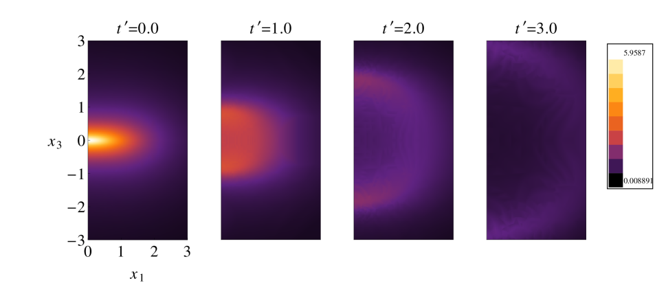
We now show how the boundary stress tensor $T^{\mathbb{R}\times S^{3}}_{\mu\nu}\equiv T_{\mu\nu}\equiv\left<T_{\mu\nu}\right>_{\text{CFT}}$ transforms under the above conformal mapping. First recall that we have effectively subtracted a term $t_{\mu\nu}=\underset{q\rightarrow 0}{\lim}{\frac{1}{q^{2}}}{}^{(q)}t_{\mu\nu}$ from $T^{\mathbb{R}\times S^{3}}_{\mu\nu}$, by removing the term ${}^{(q)}t_{\mu\nu}$ from the quasi-local stress tensor (21) prior to taking the boundary limit. Due to this subtraction, the correct rule for obtaining the stress tensor $T^{\mathbb{R}^{3,1}}_{ab}$ on Minkowski space obtained via the conformal mapping described above is:

$$T^{\mathbb{R}^{3,1}}_{ab}=W^{-2}{\partial x^{\mu}\over\partial x^{a}}{\partial x^{\nu}\over\partial x^{b}}T^{\mathbb{R}\times S^{3}}_{\mu\nu}\,.$$ (114)

Had we not subtracted $t_{\mu\nu}$ in our calculation of $T^{\mathbb{R}\times S^{3}}_{\mu\nu}$, we would have had to include an additional term in (114), identified in Skenderis (2001) as a consequence of the holographic Weyl anomaly. In other words, the full stress tensor is not a covariant object under the family of bulk diffeomorphisms that induce conformal transformations on the boundary. On the CFT, this anomalous term is not surprising: it is simply the usual Schwarzian derivative term that appears when one passes the stress tensor of an even-dimensional CFT through a conformal transformation. From the bulk perspective, the anomaly originates from picking out a particular foliation before taking the boundary limit (19).

To explicitly see that the rule (114) results in the correct stress tensor on Minkowski space, it is instructive to consider the unsubtracted boundary stress tensor $T^{0}_{\mu\nu}=\underset{q\rightarrow 0}{\lim}{\frac{1}{q^{2}}}{}^{(q)}T^{0}_{\mu\nu}$. Since the anomalous term does not depend on the bulk dynamical variables $\bar{g}_{\mu\nu},\bar{H}_{\mu},\bar{\phi}$, it suffices to evaluate this object in the case where $\bar{g}_{\mu\nu}=0,\bar{H}_{\mu}=0,\bar{\phi}=0$. Performing this calculation in global AdS₅, we use the foliator $q=1-\rho=1/(1+r)$ and find that $T^{0,\mathbb{R}\times S^{3}}_{\mu\nu}=t_{\mu\nu}$. On the other hand, this same calculation on the Poincaré patch involves the foliator $q=1/(\sqrt{(}1+r^{2}/L^{2})\cos(t/L)+r/L\sin\chi\cos\theta)$ (essentially the Poincaré radial coordinate) and one finds that $T^{0,\mathbb{R}^{3,1}}_{\mu\nu}=0$. This calculation concretely demonstrates that $T^{0}_{\mu\nu}$ is not a covariant object. It additionally shows that by subtracting $t_{\mu\nu}$ from the boundary stress tensor on $\mathbb{R}\times S^{3}$, one may pass the rest of the stress tensor $T^{\mathbb{R}\times S^{3}}_{\mu\nu}=T^{0,\mathbb{R}\times S^{3}}_{\mu\nu}-t_{\mu\nu}$ through the tensorial rule (114) and obtain the correct stress tensor on $\mathbb{R}^{3,1}$.

If we now take the stress tensor $T^{\mathbb{R}\times S^{3}}_{\mu\nu}$ to have an inviscid hydrodynamical form $T^{\mathbb{R}\times S^{3}}_{\mu\nu}=\epsilon u_{\mu}u_{\nu}+\epsilon\perp_{\mu\nu}/3$ as was demonstrated in Sec. VI.5, then one can straightforwardly show that $u^{\mathbb{R}^{3,1}}_{a}=W{\partial x^{\mu}\over\partial x^{a}}u^{\mathbb{R}\times S^{3}}_{\mu}$ and $\epsilon^{\mathbb{R}^{3,1}}=W^{-4}\epsilon^{\mathbb{R}\times S^{3}}$. Up to a constant factor specifying the number of degrees of freedom, the temperature of a conformal fluid is $T=\epsilon^{1/4}$. Setting $L=1$, the quantity we are going to plot is

$$T\equiv W^{-1}\epsilon^{1/4}\,,$$ (115)

where $T=T^{\mathbb{R}^{3,1}}$ is (up to the aforementioned constant factor) the temperature in Minkowski space and $\epsilon=\epsilon^{\mathbb{R}\times S^{3}}$ is the energy density on $\mathbb{R}\times S^{3}$.

We are justified in plotting temperature starting at Minkowski time $t^{\prime}=0$ because, by construction, our initial data perfectly conforms to the inviscid hydrodynamic ansatz. Moreover, again by construction, the velocity field vanishes exactly on the initial timeslice. Thus we are describing a version of the Landau-Khalatnikov full-stopping scenario Landau (1953); Khalatnikov (1954), but with radial flow explicitly included. The results of section VI.5, in particular Figs. 20 and 21, show that hydrodynamics remains approximately valid throughout the evolution, with modest contributions from shear viscosity and small contributions from second-order transport coefficients.

The four panels of Fig. 22 shows the temperature $T$ in Minkowski space reconstructed from a simulation with initial asymmetry $w_{y}/w_{x}=32$. Each panel in Fig. 22 is taken from a $t^{\prime}=const$ slice, and at $\phi=0$ (i.e. $x_{2}=0$). Since the transformation to Minkowski space preserves the original $\phi$-symmetry in global AdS, one can recover the full spatial profile by simply rotating each of these $x_{1}-x_{3}$ profiles about the $x_{3}$ axis. To quantify the initial anisotropy in the temperature profile, we use $\left<(x_{1})^{2}\right>/\left<(x_{3})^{2}\right>$, where $\left<A(x_{1},0,x_{3})\right>={\int dx_{1}dx_{3}T(x_{1},0,x_{3})^{4}A(x_{1},0,x_{3})/\int dx_{1}dx_{3}T(x_{1},0,x_{3})^{4}}$ is the energy-weighted average of some function $A(x_{1},0,x_{3})$ defined on the initial $t^{\prime}=0$ slice and at $\phi=0$. This quantity evaluates to $6.94$ for the data displayed in Fig. 22. We also calculate the widths $\delta_{1}$ and $\delta_{3}$ given by $T^{4}(\delta_{1},0,0)=T^{4}(0,0,0)/2$ and $T^{4}(0,0,\delta_{3})=T^{4}(0,0,0)/2$, then construct the ratio $(\delta_{1})^{2}/(\delta_{3})^{2}$; this evaluates to $18.7$ with the data.

VII Conclusion

We have described a generalized harmonic scheme for solving the Einstein field equations on asymptotically anti-de Sitter spacetimes in 4+1 dimensions. Though restricting to $SO(3)$ symmetry in this initial code, we expect that many of the methods developed here to achieve stable, consistent evolution will carry over to scenarios with less symmetry. This will be needed to tackle the main motivation for developing this code, namely to obtain the gravity dual to a heavy ion collision, and its subsequent quark-gluon plasma formation.

As a first application, we studied the quasi-normal ringdown of highly distorted black holes, and the corresponding behavior of the stress energy tensor of the dual CFT on the boundary of the spacetime. We find quasi-normal mode frequencies that are consistent with previously published linear modes, as well as modes that can be modeled as arising from non-linear mode-coupling. We further find purely decaying modes that we attribute to gauge. To be certain this is the case would require transforming the solution to coordinates fully compatible with perturbative calculations, which is a rather non-trivial task numerically, and so we relegate this to a future study.

The boundary stress energy tensor exhibits correspondingly large initial fluctuations, yet we find that its behavior is consistent to better than $1\%$ with that of an $\mathcal{N}=4$ SYM fluid with equation of state $\epsilon=3P$, and with corresponding transport coefficients, essentially from $t=0$ onwards. This is in contrast to the numerical results reported in Chesler and Yaffe (2011); Heller et al. (2011); Wu and Romatschke (2011); Chesler and Teaney (2011), where only after a certain time did the boundary behavior approach that of a fluid. However, those studies looked at scenarios more akin to black hole formation, i.e. beginning with states that do not contain large black holes (or black branes), with the black holes forming at later times. Such processes are expected to be dual to thermalization, whereas our study is that of equilibration beginning from an inhomogeneous though thermal state. Nevertheless, it is curious that the link between Einstein and Navier-Stokes seems to be holding even in these far-from-equilibrium scenarios, and it will be interesting in future work to explore how far this relationship extends. Recently it was shown that the Rayleigh-Plateau instability in a fluid stream and the Gregory-Laflamme instability of a black string are at least qualitiatively similar Lehner and Pretorius (2010). These findings similarly suggest that, in some situations, the physics described by the Einstein and Navier-Stokes equations could exhibit similarities even in the most non-linear, near-singular regimes.

By passing to an appropriate Minkowski patch of the boundary of global AdS₅, we are able to extract a fluid flow which starts from a compressed disk and leads to expansion both in the radial and longitudinal directions. The $SO(3)$ symmetry is still present, but as a conformal symmetry rather than an isometry of the flow. This flow exhibits the main qualitative features of the full-stopping scenario in heavy ion collisions, which, though generally considered implausible in light of asymptotic freedom, has some interesting phenomenological successes Steinberg (2005). It would be interesting to pass our flow through a hadronization algorithm and extract the rapidity distribution of produced particles. We leave this task for future work.

A further direction for future study, that could be accomplished within the simplification of the current $SO(3)$ symmetry, is to couple gravity to additional forms of matter. In the context of AdS/CFT, it is interesting to consider tachyonic scalar fields, since these amount to relevant operator insertions in the boundary CFT. As one might expect, the resulting deformation is dramatic: on the gravity side, these tachyonic scalars back-react in such a way as to significantly change the boundary conditions of the metric. The evolution of such systems in the full non-linear regime is unknown, though hopefully methods similar to those introduced here will be able to handle such spacetimes with “deformed” AAdS boundaries. These methods are also applicable to AAdS spacetimes with different boundary topology, which (with the appropriate matter content) are of interest to condensed matter applications of the duality.

Appendix A Effect of Scalar Backreaction on Metric Fall-off

Here we compute the effect that a static spherical distribution of massless scalar would have on the AAdS₅ metric. We follow the discussion in Henneaux et al. (2007). The configuration only has radial dependence $\phi=\phi(r)$, so the metric must take the form

$$ds^{2}=-\left(1+r^{2}+\mathcal{O}(r^{-1})\right)dt^{2} + \frac{1}{\left(1+r^{2}-\frac{\mu(r)}{r}\right)}dr^{2}$$ (116)

$$+ r^{2}d{\Omega_{3}}^{2}$$

where $\mu(r)$ grows slower than $r^{3}$ as $r\rightarrow\infty$ in order to preserve the value of the cosmological constant. We have set $L=1$, so that $\Lambda_{5}=-6$. In a previous section, we had used the AdS₅ Klein-Gordon equation (16) in spherical symmetry to find the general leading order behavior (17) of scalar fields in AdS₅. We now find the metric fall-off behavior when scalar back-reaction is taken into account, limiting ourselves to the $h_{\rho\rho}$ component of the metric deviation and using the compactified coordinate $\rho=r/(1+r)$. In order to find this fall-off, the strategy is to solve for $\mu(r)$ as a power series in $r$, from which we can reconstruct

$$h_{\rho\rho}=\left(\frac{\partial r}{\partial\rho}\right)^{2}h_{rr}=\frac{\mu(r)}{r}$$ (117)

where we have used $\partial r/\partial\rho=1/(1-\rho)^{2}\sim r^{2}$ along with $h_{rr}=g_{rr}-\hat{g}_{rr}$ and

$$g_{rr}=\left(1+r^{2}-\mu(r)/r\right)^{-1}=\frac{1}{r^{2}}\left[1+\frac{\mu(r)}{r^{3}}+\mathcal{O}(r^{-5})\right].$$ (118)

We can deduce the asymptotic behavior of $\mu(r)$ from the the Hamiltonian constraint

$${}^{(4)}R-2\Lambda_{5}=16\pi\rho_{E}.$$ (119)

where

$${}^{(4)}R=2\Lambda_{5}+\frac{2+r^{2}(5+3r^{2})}{(r+r^{3})^{2}}\mu^{\prime}(r)+\frac{r(5+3r^{2})}{(r+r^{3})^{2}}\mu(r)$$ (120)

is the Ricci scalar associated with the 4-metric on the slice, and

$$\rho_{E}=\frac{1}{2}(1+r^{2}-\mu(r)/r)(\phi^{\prime}(r))^{2}+\frac{1}{2}m^{2}\phi^{2}$$ (121)

is the scalar field energy density. Keeping only the terms in (119) that dominate at large $r$, we obtain the form of the Hamiltonian constraint near the boundary

$$\frac{\mu^{\prime}(r)}{r^{2}}+\frac{\mu(r)}{r}(\phi^{\prime}(r))^{2}\sim r^{2}(\phi^{\prime}(r))^{2}+m^{2}\phi^{2}.$$ (122)

The scalar field goes as $\phi(r)\sim r^{-\Delta}$ near the boundary for some $\Delta$, so we see that the right-hand-side of (122) goes as $r^{-2\Delta}$. Matching the left and right-hand sides, we conclude that

$$\mu(r)\sim r^{3-2\Delta}$$ (123)

and consequently,

$$h_{\rho\rho}\sim r^{2-2\Delta}.$$ (124)

To make use of what we have learnt, first suppose that we have a scalar with negative $m^{2}<0$. From (17) and (18), a non-zero $A$ branch describes the leading behavior for large $r$, and is defined by a fall-off power of $\Delta=\Delta_{+}=2-\sqrt{4+m^{2}}$. Then equation (124) predicts that matter backreaction induces a metric deviation $h_{\rho\rho}\sim r^{-2+2\sqrt{4+m^{2}}}$ that is larger than the vacuum metric fall-off we assumed in (IV.2) and in (IV.2). This case corresponds to a tachyonic scalar configuration. These configurations are stable in AdS as long as its mass satisfies the Breitenlohner-Freedman bound Breitenlohner and Freedman (1982) given by $-(D-1)^{2}/(4L^{2})=-4<m^{2}$ in $D=5$ dimensions: it is stable in the sense that its conserved energy functional remains positive in the function space of all fluctuations for which the energy functional remains a convergent integral. The qualitative reason for the positivity of this energy functional in AdS is that despite the negative unbounded potential of the tachyonic scalar, the positive kinetic terms in the energy functional dominate the negative potential terms so long as the scalar falls off sufficiently quickly near the boundary. We shall elaborate on the behavior of these fields in a subsequent paper.

For the present paper, we consider the case of scalars with $m^{2}\geq 0$. Again looking at (17), (18), notice that we must now turn off the $A$ branch in order to have a scalar field that vanishes at infinity, which is required for any scalar field configuration with finite energy. The result is a localized matter distribution defined by a fall-off power $\Delta=\Delta_{+}=2+\sqrt{4+m^{2}}$. Applying our result (124) to this case, we find that backreaction induces a metric deviation $h_{\rho\rho}\sim r^{-2-2\sqrt{4+m^{2}}}$ that is subleading compared to the vacuum metric fall-off (IV.2), and thus leaving it unchanged.

Appendix B Boundary Conditions for Linearized Gravitational Perturbations of AdS

Fefferman-Graham Theorem

A theorem due to Fefferman and Graham Fefferman and Graham (1985) states that a distinguished coordinate system $(z,x^{i})$ exists near the boundary of any asymptotically AdS₅ spacetime $M$ in which the metric takes the form

$$G=\frac{L^{2}}{z^{2}}\left(dz^{2}+g_{ij}dx^{i}dx^{j}\right)$$ (125)

and that there is a convergent power series solution for the $g_{ij}$ coefficients in (125) given by

$$g_{ij}=g_{(0)ij}+g_{(2)ij}z^{2}+g_{(4)ij}z^{4}+2h_{(4)ij}z^{4}\log z+\mathcal{O}(z^{6})$$ (126)

(the boundary $\partial M$ is located at $z=0$).

Let us first translate this statement in terms of global AdS₅ coordinates $(t,r,\chi,\theta,\phi)$. We follow the discussion in Skenderis (2001), though we use a different Fefferman-Graham radial coordinate $z$ from the one use there, whose relation with the global radial coordinate $r$ is given by

$$r^{2}=\frac{1}{z^{2}}\left(1-\frac{z^{2}}{4}\right)^{2}.$$ (127)

To leading order, this relation between $z$ and $r$ near the boundary at $z=0$, or equivalently $r\rightarrow\infty$, simply reads

$$z=\frac{1}{r}+\mathcal{O}(1/r^{2}).$$ (128)

In terms of the global coordinate $q=1/(1+r)$ introduced in Sec. II.5, to leading-order we have $z=1/r+\mathcal{O}(1/r^{2})=q+\mathcal{O}(q^{2})$ near the $q=0$ boundary. So the Fefferman-Graham theorem’s power series solution in these coordinates reads just like (126), replacing $z$ by $q$

$$g_{ij}=g_{(0)ij}+g_{(2)ij}q^{2}+g_{(4)ij}q^{4}+2h_{(4)ij}q^{4}\log q+\mathcal{O}(q^{6})$$ (129)

(the boundary $\partial M$ is located at $q=0$).

The $g_{(0)ij}$ corresponds to the non-radial components of the pure AdS₅ metric. The $g_{(2)ij}$ can be expressed, as was done explicitly in de Haro et al. (2001), in terms of the Ricci tensor $R_{(0)ij}$ and the scalar curvature $R_{(0)}$ constructed from $g_{(0)ij}$, and is thus fixed. The leading-order dynamics then first appears in the terms controlled by $g_{(4)ij}$. Inspecting (129), this implies that the leading-order asymptotics is $G_{ij}\sim q^{2}$, in agreement with the boundary conditions we wrote down in Sec. IV.2.

Ishibashi-Wald Boundary Conditions

Here we show how our metric boundary conditions relate to those derived by Ishibashi and Wald in Ishibashi and Wald (2004). Working perturbatively, they derive conditions under which a metric perturbation must have its boundary behavior enforced by explicit boundary conditions. The fields governing the perturbations, which we collectively denote by $f$, are decomposed in terms of spherical harmonics $\mathbb{S}_{k}(\Omega^{i})$ according to

$$f=\frac{1}{r^{3/2}}\sum_{k_{S}}\Phi_{k}(t,r)\mathbb{S}_{k}(\Omega^{i}).$$ (130)

The $\Phi$ fields for the tensor and vectors modes of the gravitational perturbations are shown to require no boundary conditions at infinity (see Proposition 3.1 and its preceding discussion in Ishibashi and Wald (2004)). However, the scalar modes of the gravitational perturbations require boundary conditions, and their corresponding $\Phi$ are shown to behave asymptotically as

$$\Phi=F_{0}(r)\left[2a_{0}\log(1/r)+b_{0}+2L^{2}/r^{2}\log(1/r)+...\right]$$ (131)

where the function $F_{0}(r)$ is asymptotically given by

$$F_{0}(r)\sim\frac{1}{r^{1/2}}.$$ (132)

In terms of the global coordinate $q$, the implication is that for the scalar modes of the gravitational perturbations the near-boundary behavior is

$$G_{ij}\sim 2a_{0}q^{2}\log(q)+b_{0}q^{2}+2c_{0}q^{4}\log(q)+...$$ (133)

For the scalar modes, imposing boundary conditions amounts to setting the ratio $b_{0}/a_{0}$. Comparing (133) to (125),(129), we see that the choice picked out by coordinates that are Fefferman-Graham-like near the boundary is $b_{0}/a_{0}\rightarrow\infty$ i.e. $a_{0}=0$. This removes the logarithmic branch controlled by $a_{0}$, so the leading-order asymptotics is $G_{ij}\sim q^{2}$, as desired.

Appendix C Tables of Scalar Quasinormal Mode Frequencies

	fund.	k=0	k=2	k=4
	$\frac{r_{h}}{L}$=12.2	$(2.95\pm 0.13)\frac{r_{h}}{L}-i(2.67\pm 0.02)\frac{r_{h}}{L}$	$(3.96\pm 0.03)\frac{r_{h}}{L}-i(2.33\pm 0.07)\frac{r_{h}}{L}$	$(4.93\pm 0.007)\frac{r_{h}}{L}-i(1.83\pm 0.05)\frac{r_{h}}{L}$
	$\frac{r_{h}}{L}$=11.3	$(2.95\pm 0.14)\frac{r_{h}}{L}-i(2.64\pm 0.04)\frac{r_{h}}{L}$	$(3.94\pm 0.02)\frac{r_{h}}{L}-i(2.30\pm 0.08)\frac{r_{h}}{L}$	$(4.90\pm 0.003)\frac{r_{h}}{L}-i(1.80\pm 0.04)\frac{r_{h}}{L}$
	$\frac{r_{h}}{L}$=10.5	$(2.96\pm 0.14)\frac{r_{h}}{L}-i(2.64\pm 0.05)\frac{r_{h}}{L}$	$(3.95\pm 0.01)\frac{r_{h}}{L}-i(2.29\pm 0.08)\frac{r_{h}}{L}$	$(4.92\pm 0.002)\frac{r_{h}}{L}-i(1.78\pm 0.04)\frac{r_{h}}{L}$
	$\frac{r_{h}}{L}$=9.0	$(2.99\pm 0.15)\frac{r_{h}}{L}-i(2.63\pm 0.07)\frac{r_{h}}{L}$	$(3.95\pm 0.002)\frac{r_{h}}{L}-i(2.26\pm 0.09)\frac{r_{h}}{L}$	$(4.90\pm 0.02)\frac{r_{h}}{L}-i(1.72\pm 0.02)\frac{r_{h}}{L}$
	$\frac{r_{h}}{L}$=6.5	$(3.06\pm 0.14)\frac{r_{h}}{L}-i(2.62\pm 0.14)\frac{r_{h}}{L}$	$(3.96\pm 0.05)\frac{r_{h}}{L}-i(2.23\pm 0.07)\frac{r_{h}}{L}$	$(4.80\pm 0.01)\frac{r_{h}}{L}-i(1.65\pm 0.003)\frac{r_{h}}{L}$
	$\frac{r_{h}}{L}$=5.0	$(3.11\pm 0.09)\frac{r_{h}}{L}-i(2.62\pm 0.20)\frac{r_{h}}{L}$	$(3.94\pm 0.05)\frac{r_{h}}{L}-i(2.21\pm 0.04)\frac{r_{h}}{L}$	$(4.79\pm 0.08)\frac{r_{h}}{L}-i(1.60\pm 0.02)\frac{r_{h}}{L}$
	$\frac{r_{h}}{L}$=4.5	$(3.18\pm 0.06)\frac{r_{h}}{L}-i(2.67\pm 0.22)\frac{r_{h}}{L}$	$(4.00\pm 0.06)\frac{r_{h}}{L}-i(2.24\pm 0.04)\frac{r_{h}}{L}$	$(4.87\pm 0.11)\frac{r_{h}}{L}-i(1.69\pm 0.04)\frac{r_{h}}{L}$
	$\frac{r_{h}}{L}$=4.0	$(3.21\pm 0.001)\frac{r_{h}}{L}-i(2.67\pm 0.23)\frac{r_{h}}{L}$	$(3.99\pm 0.06)\frac{r_{h}}{L}-i(2.24\pm 0.03)\frac{r_{h}}{L}$	$(4.83\pm 0.12)\frac{r_{h}}{L}-i(1.76\pm 0.04)\frac{r_{h}}{L}$
	$\frac{r_{h}}{L}$=3.3	$(3.33\pm 0.08)\frac{r_{h}}{L}-i(2.71\pm 0.20)\frac{r_{h}}{L}$	$(4.05\pm 0.08)\frac{r_{h}}{L}-i(2.27\pm 0.03)\frac{r_{h}}{L}$	$(4.9\pm 0.1)\frac{r_{h}}{L}-i(1.89\pm 0.05)\frac{r_{h}}{L}$

Table 4: The fundamental ($n=0$) quasi-normal mode frequencies $\omega_{r}-i\omega_{i}$ extracted from the scalar field variable $\bar{\phi}$, from evolution of initial data as described in Sec. VI.2. These are shown for various horizon radii $r_{h}$ of the final state AdS-Schwarzschild black hole with $SO(4)$ quantum numbers $k\geq 0,l=0,m=0$. Uncertainties are estimated from convergence studies.

	$1^{st}$ overt.	k=0	k=2	k=4
	$\frac{r_{h}}{L}$=12.2	$(5.66\pm 0.24)\frac{r_{h}}{L}-i(2.90\pm 0.28)\frac{r_{h}}{L}$	$(6.36\pm 0.26)\frac{r_{h}}{L}-i(3.28\pm 0.15)\frac{r_{h}}{L}$	$(7.60\pm 0.17)\frac{r_{h}}{L}-i(4.11\pm 0.17)\frac{r_{h}}{L}$
	$\frac{r_{h}}{L}$=11.3	$(5.65\pm 0.27)\frac{r_{h}}{L}-i(2.91\pm 0.30)\frac{r_{h}}{L}$	$(6.36\pm 0.31)\frac{r_{h}}{L}-i(3.32\pm 0.16)\frac{r_{h}}{L}$	$(7.59\pm 0.23)\frac{r_{h}}{L}-i(4.31\pm 0.14)\frac{r_{h}}{L}$
	$\frac{r_{h}}{L}$=10.5	$(5.69\pm 0.30)\frac{r_{h}}{L}-i(2.94\pm 0.32)\frac{r_{h}}{L}$	$(6.41\pm 0.35)\frac{r_{h}}{L}-i(3.37\pm 0.14)\frac{r_{h}}{L}$	$(7.63\pm 0.26)\frac{r_{h}}{L}-i(4.56\pm 0.14)\frac{r_{h}}{L}$
	$\frac{r_{h}}{L}$=9.0	$(5.76\pm 0.38)\frac{r_{h}}{L}-i(3.00\pm 0.36)\frac{r_{h}}{L}$	$(6.50\pm 0.45)\frac{r_{h}}{L}-i(3.52\pm 0.16)\frac{r_{h}}{L}$	$(7.74\pm 0.39)\frac{r_{h}}{L}-i(5.22\pm 0.10)\frac{r_{h}}{L}$
	$\frac{r_{h}}{L}$=6.5	$(5.98\pm 0.62)\frac{r_{h}}{L}-i(3.19\pm 0.42)\frac{r_{h}}{L}$	$(6.78\pm 0.71)\frac{r_{h}}{L}-i(4.02\pm 0.08)\frac{r_{h}}{L}$	$(8.04\pm 0.79)\frac{r_{h}}{L}-i(7.92\pm 0.41)\frac{r_{h}}{L}$
	$\frac{r_{h}}{L}$=5.0	$(6.20\pm 0.96)\frac{r_{h}}{L}-i(3.54\pm 0.51)\frac{r_{h}}{L}$	$(7.15\pm 1.02)\frac{r_{h}}{L}-i(4.96\pm 0.17)\frac{r_{h}}{L}$	$(7.40\pm 1.43)\frac{r_{h}}{L}-i(8.69\pm 1.87)\frac{r_{h}}{L}$
	$\frac{r_{h}}{L}$=4.5	$(6.41\pm 1.13)\frac{r_{h}}{L}-i(3.82\pm 0.57)\frac{r_{h}}{L}$	$(7.45\pm 1.19)\frac{r_{h}}{L}-i(5.61\pm 0.32)\frac{r_{h}}{L}$	$(7.63\pm 2.19)\frac{r_{h}}{L}-i(8.78\pm 1.74)\frac{r_{h}}{L}$
	$\frac{r_{h}}{L}$=4.0	$(6.58\pm 1.36)\frac{r_{h}}{L}-i(4.24\pm 0.68)\frac{r_{h}}{L}$	$(7.71\pm 1.44)\frac{r_{h}}{L}-i(6.67\pm 0.76)\frac{r_{h}}{L}$	$(7.77\pm 1.82)\frac{r_{h}}{L}-i(9.94\pm 3.02)\frac{r_{h}}{L}$
	$\frac{r_{h}}{L}$=3.3	$(7.02\pm 1.78)\frac{r_{h}}{L}-i(5.34\pm 1.04)\frac{r_{h}}{L}$	$(8.04\pm 1.74)\frac{r_{h}}{L}-i(9.35\pm 2.38)\frac{r_{h}}{L}$	$(7.68\pm 1.32)\frac{r_{h}}{L}-i(12.7\pm 4.7)\frac{r_{h}}{L}$

Table 5: The first overtone ($n=1$) quasi-normal mode frequencies $\omega_{r}-i\omega_{i}$ extracted from the scalar field variable $\bar{\phi}$, from evolution of initial data as described in Sec. VI.2. These are shown for various horizon radii $r_{h}$ of the final state AdS-Schwarzschild black hole and for harmonics with $SO(4)$ quantum numbers $k\geq 0,l=0,m=0$. Uncertainties are estimated from convergence studies.

References

- Maldacena (1998) J. M. Maldacena, Adv. Theor. Math. Phys. 2, 231 (1998), eprint hep-th/9711200.
- Gubser et al. (1998) S. Gubser, I. R. Klebanov, and A. M. Polyakov, Phys.Lett. B428, 105 (1998), eprint hep-th/9802109.
- Witten (1998) E. Witten, Adv. Theor. Math. Phys. 2, 253 (1998), eprint hep-th/9802150.
- Gubser and Karch (2009) S. S. Gubser and A. Karch, Ann. Rev. Nucl. Part. Sci. 59, 145 (2009), eprint 0901.0935.
- Herzog (2009) C. P. Herzog, J.Phys.A A42, 343001 (2009), eprint 0904.1975.
- Hartnoll (2009) S. A. Hartnoll, Class.Quant.Grav. 26, 224002 (2009), eprint 0903.3246.
- McGreevy (2010) J. McGreevy, Adv. High Energy Phys. 2010, 723105 (2010), eprint 0909.0518.
- Sachdev (2010) S. Sachdev (2010), eprint 1002.2947.
- Gubser (2010a) S. S. Gubser (2010a), eprint 1012.5312.
- Horowitz (2010) G. T. Horowitz (2010), eprint 1002.1722.
- Gubser (2011) S. S. Gubser (2011), eprint 1103.3636.
- Pretorius (2007) F. Pretorius (2007), eprint 0710.1338.
- Duez (2010) M. D. Duez, Class.Quant.Grav. 27, 114002 (2010), eprint 0912.3529.
- Campanelli et al. (2010) M. Campanelli, C. O. Lousto, B. C. Mundim, H. Nakano, Y. Zlochower, et al., Class.Quant.Grav. 27, 084034 (2010), eprint 1001.3834.
- Centrella et al. (2010) J. Centrella, J. G. Baker, B. J. Kelly, and J. R. van Meter, Rev. Mod. Phys. 82, 3069 (2010), eprint 1010.5260.
- Pretorius and Choptuik (2000) F. Pretorius and M. W. Choptuik, Phys.Rev. D62, 124012 (2000), eprint gr-qc/0007008.
- Husain and Olivier (2001) V. Husain and M. Olivier, Class.Quant.Grav. 18, L1 (2001), eprint gr-qc/0008060.
- Hwang et al. (2011) D.-i. Hwang, H. Kim, and D.-h. Yeom (2011), eprint 1105.1371.
- Bizon and Rostworowski (2011) P. Bizon and A. Rostworowski (2011), eprint 1104.3702.
- Garfinkle and Pando Zayas (2011) D. Garfinkle and L. A. Pando Zayas (2011), eprint 1106.2339.
- Husain et al. (2003) V. Husain, G. Kunstatter, B. Preston, and M. Birukou, Class. Quant. Grav. 20, L23 (2003), eprint gr-qc/0210011.
- Birukou et al. (2002) M. Birukou, V. Husain, G. Kunstatter, E. Vaz, and M. Olivier, Phys.Rev. D65, 104036 (2002).
- Chesler and Yaffe (2011) P. M. Chesler and L. G. Yaffe, Phys. Rev. Lett. 106, 021601 (2011), eprint 1011.3562.
- Wu and Romatschke (2011) B. Wu and P. Romatschke (2011), eprint 1108.3715.
- Chesler and Teaney (2011) P. M. Chesler and D. Teaney (2011), eprint 1112.6196.
- Heller et al. (2011) M. P. Heller, R. A. Janik, and P. Witaszczyk (2011), eprint 1103.3452.
- Pretorius (2005a) F. Pretorius, Class.Quant.Grav. 22, 425 (2005a), eprint gr-qc/0407110.
- Pretorius (2005b) F. Pretorius, Phys.Rev.Lett. 95, 121101 (2005b), eprint gr-qc/0507014.
- Gubser et al. (2008) S. S. Gubser, S. S. Pufu, and A. Yarom, Phys. Rev. D78, 066014 (2008), eprint 0805.1551.
- Gubser et al. (2009) S. S. Gubser, S. S. Pufu, and A. Yarom, JHEP 11, 050 (2009), eprint 0902.4062.
- Kovtun and Starinets (2006) P. Kovtun and A. Starinets, Phys.Rev.Lett. 96, 131601 (2006), eprint hep-th/0602059.
- Janik and Peschanski (2006) R. A. Janik and R. B. Peschanski, Phys. Rev. D74, 046007 (2006), eprint hep-th/0606149.
- Friess et al. (2007) J. J. Friess, S. S. Gubser, G. Michalogiorgakis, and S. S. Pufu, JHEP 04, 080 (2007), eprint hep-th/0611005.
- Ishibashi and Wald (2004) A. Ishibashi and R. M. Wald, Class.Quant.Grav. 21, 2981 (2004), eprint hep-th/0402184.
- Henneaux and Teitelboim (1985) M. Henneaux and C. Teitelboim, Commun. Math. Phys. 98, 391 (1985).
- Fefferman and Graham (1985) C. Fefferman and C. R. Graham, Astérisque pp. 95–116 (1985), ISSN 0303-1179, the mathematical heritage of Élie Cartan (Lyon, 1984).
- de Haro et al. (2001) S. de Haro, S. N. Solodukhin, and K. Skenderis, Commun.Math.Phys. 217, 595 (2001), eprint hep-th/0002230.
- Henneaux et al. (2007) M. Henneaux, C. Martinez, R. Troncoso, and J. Zanelli, Annals Phys. 322, 824 (2007), eprint hep-th/0603185.
- Papadimitriou and Skenderis (2005) I. Papadimitriou and K. Skenderis, JHEP 0508, 004 (2005), eprint hep-th/0505190.
- Brown and York (1993) J. D. Brown and J. W. York, Jr., Phys. Rev. D47, 1407 (1993), eprint gr-qc/9209012.
- Balasubramanian and Kraus (1999) V. Balasubramanian and P. Kraus, Commun. Math. Phys. 208, 413 (1999), eprint hep-th/9902121.
- Arnowitt et al. (1962) R. L. Arnowitt, S. Deser, and C. W. Misner (1962), gravitation: an introduction to current research, Louis Witten ed. (Wilew 1962), chapter 7, pp 227-265, eprint gr-qc/0405109.
- Gourgoulhon (2007) E. Gourgoulhon, J. Phys. Conf. Ser. 91, 012001 (2007), eprint 0704.0149.
- Garfinkle (2002) D. Garfinkle, APS Meeting Abstracts pp. 12004–+ (2002).
- Lindblom et al. (2006) L. Lindblom, M. A. Scheel, L. E. Kidder, R. Owen, and O. Rinne, Class.Quant.Grav. 23, S447 (2006), eprint gr-qc/0512093.
- Friedrich (1985) H. Friedrich, Communications in Mathematical Physics 100, 525 (1985).
- Gundlach et al. (2005) C. Gundlach, J. M. Martin-Garcia, G. Calabrese, and I. Hinder, Class. Quant. Grav. 22, 3767 (2005), eprint gr-qc/0504114.
- Garfinkle and Duncan (2001) D. Garfinkle and G. C. Duncan, Phys. Rev. D63, 044011 (2001), eprint gr-qc/0006073.
- Hubeny et al. (2011) V. E. Hubeny, S. Minwalla, and M. Rangamani (2011), eprint 1107.5780.
- Stephani et al. (2003) H. Stephani, D. Kramer, M. Maccallum, C. Hoenselaers, and E. Herlt, Exact Solutions of Einstein’s Field Equations (Cambridge University Press, Cambridge, UK, 2003).
- Kreiss and Oliger (1973) H.-O. Kreiss and J. Oliger, Global Atmospheric Research Program Publication 10 (1973).
- Calabrese et al. (2004) G. Calabrese, L. Lehner, O. Reula, O. Sarbach, and M. Tiglio, Class.Quant.Grav. 21, 5735 (2004), eprint gr-qc/0308007.
- Pfeiffer and York (2005) H. P. Pfeiffer and J. W. York, Jr., Phys. Rev. Lett. 95, 091101 (2005), eprint gr-qc/0504142.
- Horowitz and Hubeny (2000) G. T. Horowitz and V. E. Hubeny, Phys. Rev. D62, 024027 (2000), eprint hep-th/9909056.
- Cardoso et al. (2003) V. Cardoso, R. Konoplya, and J. P. S. Lemos, Phys. Rev. D68, 044024 (2003), eprint gr-qc/0305037.
- Kovtun and Starinets (2005) P. K. Kovtun and A. O. Starinets, Phys. Rev. D72, 086009 (2005), eprint hep-th/0506184.
- Teaney (2006) D. Teaney, Phys. Rev. D74, 045025 (2006), eprint hep-ph/0602044.
- Berti et al. (2009) E. Berti, V. Cardoso, and A. O. Starinets, Class. Quant. Grav. 26, 163001 (2009), eprint 0905.2975.
- Avery (2000) J. Avery, Hyperspherical Harmonics and Generalized Sturmians (Kluwer Academic Publishers, Dordrecht, Netherlands, 2000).
- Kodama and Ishibashi (2003) H. Kodama and A. Ishibashi, Prog. Theor. Phys. 110, 701 (2003), eprint hep-th/0305147.
- Emparan (2011) R. Emparan (2011), eprint 1106.2021.
- Loganayagam (2008) R. Loganayagam, JHEP 05, 087 (2008), eprint 0801.3701.
- Gubser (2010b) S. S. Gubser, Phys. Rev. D82, 085027 (2010b), eprint 1006.0006.
- Gubser and Yarom (2011) S. S. Gubser and A. Yarom, Nucl. Phys. B846, 469 (2011), eprint 1012.1314.
- Staig and Shuryak (2011a) P. Staig and E. Shuryak, Phys. Rev. C84, 044912 (2011a), eprint 1105.0676.
- Staig and Shuryak (2011b) P. Staig and E. Shuryak, J. Phys. G38, 124039 (2011b), eprint 1106.3243.
- Skenderis (2001) K. Skenderis, Int. J. Mod. Phys. A16, 740 (2001), eprint hep-th/0010138.
- Landau (1953) L. D. Landau, Izv. Akad. Nauk SSSR Ser. Fiz. 17, 51 (1953).
- Khalatnikov (1954) I. M. Khalatnikov, ZhETF 27, 529 (1954).
- Lehner and Pretorius (2010) L. Lehner and F. Pretorius, Phys.Rev.Lett. 105, 101102 (2010), eprint 1006.5960.
- Steinberg (2005) P. Steinberg, Acta Phys. Hung. A24, 51 (2005), eprint nucl-ex/0405022.
- Breitenlohner and Freedman (1982) P. Breitenlohner and D. Z. Freedman, Phys. Lett. B115, 197 (1982).