A Survey of Heavy Quark Theory for PDF Analyses

Abstract

We survey some of the recent developments in the extraction and application of heavy quark Parton Distribution Functions (PDFs). We also highlight some of the key HERA measurements which have contributed to these advances.

Two Decades of HERA physics

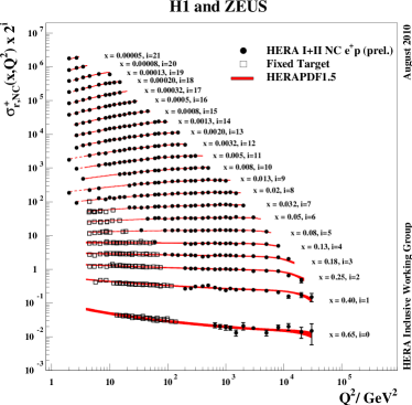
Figure 1: $e^{+}p$ NC cross section for the combined HERA data as compared with the HERAPDF1.5 fit as a function of $Q^{2}$ for different values of $x$. (Figure from H1prelim-10-142 & ZEUS-prel-10-018.)

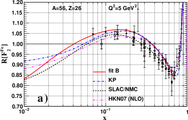
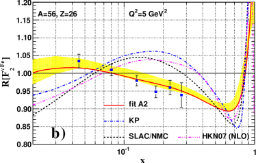
Figure 2: The computed nuclear correction ratio, $F_{2}^{Fe}/F_{2}^{N}$, as a function of $x$ for $Q^{2}=5\,{\rm GeV}^{2}$. Figure-a) shows the fit (fit B from Ref. [16]) using charged-lepton–nucleus ($\ell^{\pm}A$) and DY data whereas Figure-b) shows the fit using neutrino-nucleus ($\nu A$) data (fit A2 from Ref. [2]). Both fits are compared with the SLAC/NMC parameterization [16], as well as fits from Kulagin-Petti (KP) (Ref. [3, 4]) and Hirai et al. (HKN07), (Ref. [5]). The data points displayed in Figure-a) come from a selection of SLAC and BCDMS data. [6, 7, 8, 9, 10, 11, 12].

The HERA electron-proton collider ring began its physics program in 1992 and completed accelerator operations in 2007. The data collected by the HERA facility allowed for physics studies over a tremendously expanded kinematic region compared to the previous fixed-target experiments. This point is illustrated in Figure 1 where we display the $e^{+}p$ Neutral Current (NC) cross section vs. $Q^{2}$ for the HERA data (runs I and II) together with the fixed-target data. We observe that the HERA data allows us to extend our reach in $Q^{2}$ by more than two decades for large to intermediate $x$ values, and also extends the small $x$ region down to $\sim 10^{-5}$.

Additionally, the large statistics and reduced systematics of the experimental data demand that the theoretical predictions keep pace. Over the lifetime of HERA we have seen many of the theoretical calculations advanced from Leading-Order (LO), to Next-to-Leading-Order (NLO), and some even to Next-to-Next-to-Leading-Order (NNLO).

As the required theoretical precision has increased, it has been necessary to revisit the many inputs and assumptions which are used in the calculations. We will examine the role that the heavy quarks–and their associated masses–play in these calculations, both for the evolution of the parton distribution functions (PDFs) and also the hard-scattering cross sections.

Determining the Heavy Quark PDFs

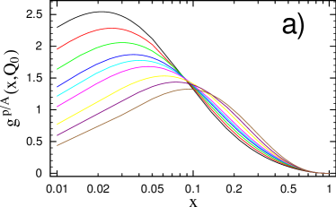
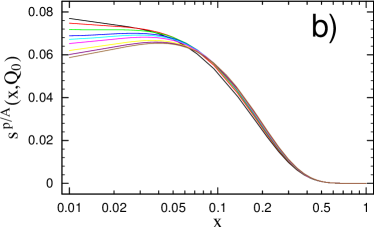
Figure 3: The a) gluon $x\,g(x,Q_{0})$ and b) strange quark $x\,s(x,Q_{0})$ nuclear PDFs as a function of $x$ for a selection of nuclear A values $\{1,2,4,9,12,27,56,108,207\}$ (from top to bottom at $x=0.01$). We choose $Q_{0}=1.3\,{\rm GeV}$.

HERA’s reach to larger $Q^{2}$ and smaller $x$ values takes us to a new kinematic region where the heavy quarks ($s,c,b$) play a more important role. For example, the strange and charm quark contributions to $F_{2}$ at small $x$ values can be 30% or more of the total inclusive result. To make high-precision predictions for the structure functions we must therefore be capable of reducing the uncertainty of these heavy quark contributions; this requires, in part, precise knowledge of the PDFs which enter the calculation.

The determination of the PDFs requires a variety of data sets which constrain different linear combinations of the PDF flavors. For example, Neutral Current (NC) charged-lepton Deeply Inelastic Scattering (DIS) (at low $Q^{2}$) probes a charge weighted combination $\sim 4u+d+s+4c$. In contrast, charged current (CC) neutrino DIS can probe different flavor combinations via $W^{\pm}$-boson exchange; additionally the neutrino measurements can probe the parity-violating $xF_{3}$ structure function.

Nuclear Correction Factors

The most precise determination of the strange quark PDF component comes from neutrino–nucleon ($\nu$-N) di-muon DIS ($\nu N\to\mu^{-}\mu^{+}X$) process. This (dominantly) takes place via the Cabibbo favored partonic process $\nu s\to\mu^{-}c$ followed by a semi-leptonic charm decay. As the neutrino cross section is small, this measurement is typically made using heavy nuclear targets (Fe, Pb), so nuclear corrections must be applied to relate the results to a proton or isoscalar nuclei.

However, recent analyses indicate that the nuclear corrections for the $\nu$-N and $\ell^{\pm}$-N DIS processes are different [1]; hence, this introduces an uncertainty into the strange quark PDF extraction which was not realized previously. Figure 2 displays the nuclear correction factors obtained for the a) $\ell^{\pm}$-N and b) $\nu$-N processes. Here, we plot the ratio of $F_{2}^{Fe}$ to an isoscalar $F_{2}^{N}$ as a function of $x$ for the $Q^{2}$ value indicated.

The contrast between the charged-lepton ($\ell^{\pm}A$) case and the neutrino ($\nu A$) case in Figure 2 is striking; while the charged-lepton results generally align with the SLAC/NMC [2], KP [3, 4] and HKN [5] determinations, the neutrino results clearly yield different behavior in the intermediate $x$-region. We emphasize that both the charged-lepton and neutrino results are not a model—they come directly from global fits to the data. To emphasize this point, we have superimposed illustrative data points in the figures; these are simply a) the SLAC and BCDMS data [6, 7, 8, 9, 10, 11, 12] or b) the $\nu A$ DIS data [13] scaled by the appropriate structure function, calculated with the proton PDF of Ref. [2].

The mis-match between the results in charged-lepton and neutrino DIS is particularly interesting given that there has been a long-standing “tension” between the light-target charged-lepton data and the heavy-target neutrino data in the historical fits [14, 15]. This study demonstrates that the tension is not only between charged-lepton light-target data and neutrino heavy-target data, but we now observe this phenomenon in comparisons between neutrino and charged-lepton heavy-target data.

The nCTEQ PDFs

The above example underscores the importance of a comprehensive treatment of the nuclear corrections to achieve the precision demanded by the current precision data. To move toward this goal, the nCTEQ project was developed to extend the global analysis framework of the traditional CTEQ proton PDFs to incorporate a broader set of nuclear data thereby extracting the PDFs of a nuclear target. In essence, a nuclear PDF not only depends on the momentum fraction $x$ and energy scale $Q$, but also on the nuclear “A” value: $f(x,Q,A)$. The structure of the nCTEQ analysis is closely modeled on that of the proton global analysis; in fact, the nuclear parameterizations are designed efficiently to make use of the proton limit (A=1) as a “boundary condition” to help constrain the fit.

In Figure 3 we display the gluon and strange nuclear PDFs as a function of $x$ for a selection of nuclear A values. We observe that for $x\simeq 0.01$ the nuclear modifications for the strange quark can be $\sim$25%, and for the gluon can be even larger. The details of the nuclear PDF analysis is discussed in Refs. [1, 16, 2]

The nCTEQ web-page contains 19 families of nPDF grid files which may be used to explore the variation due to the different data sets and kinematic cuts. In particular, there is a collections of nPDFs which interpolate between that of Figure 2-a) which uses the charged-lepton–nucleus ($\ell^{\pm}A$) data and of Figure 2-b) which uses the neutrino-nucleus ($\nu A$) data.

The Strange Quark PDF

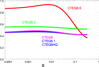
Figure 4: $\kappa(x)$ vs. $x$ for $Q=1.5$ GeV for a selection of PDFs, where we define $\kappa(x)=2s(x)/(\bar{u}(x)+\bar{d}(x))$

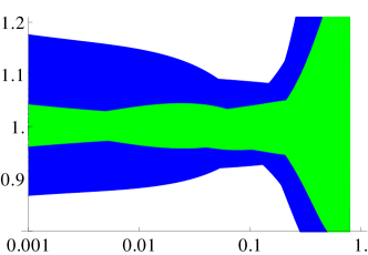
Figure 5: Relative uncertainty of the strange quark PDF as a function of $x$ for $Q=2$ GeV. The inner band is for the CTEQ6.1 PDF set, and the outer band is for the CTEQ6.6 PDF set. The band is computed as $s_{i}(x)/s_{0}(x)$ where $s_{0}(x)$ is the central PDF for each set; for CTEQ6.1, $i=[1,40]$, and for CTEQ6.6, $i=[1,44]$.

We now compare a selection of $s(x)$ distributions to gain a better understanding of the uncertainties arising from the nuclear correction factors used to analyze the $\nu$N DIS. One measure of the strange quark content of the proton is to compare $s(x)$ with the average up-quark and down-quark sea PDFs: $(\bar{u}(x)+\bar{d}(x))/2$. Thus, we define the ratio $\kappa(x)=2s(x)/(\bar{u}(x)+\bar{d}(x))$. If we had exact $SU(3)$ flavor symmetry, we would expect $\kappa=1$; the extent to which $\kappa$ is below one measures the suppression of the strange quark as compared to the up and down sea. In Figure 4 we display $\kappa(x)$ for some recent CTEQ PDFs and note that $\kappa(x)$ has a large variation, especially at small $x$ values. This reflects, in part, the fact that the strange quark is poorly constrained for $x\mathrel{\hbox to0.0pt{\lower 4.0pt\hbox{\hskip 1.0pt$\sim$}\hss}\raise 1.0pt\hbox{$<$}}0.1$. For the CTEQ6, 6HQ, 6.1, and 6.5 PDF sets, the strange quark was arbitrarily set to $\sim 1/2$ the average of the up and down sea-quarks. For the CTEQ6.6 PDF set, the strange quark was allowed additional freedom; this is reflected in Figure 5 which compares the relative uncertainty of the strange quark in the 6.1 and 6.6 PDF sets.

$W/Z$ at the LHC

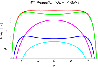
Figure 6: The differential cross section ($d\sigma/dy$) for $W^{+}$ production at the LHC ($\sqrt{s}$=14TeV) as a function of rapidity $y$. The partonic contributions are also displayed. At $y=0$, the contributions (from top to bottom) are {$total$, $u\bar{d}$, $c\bar{s}$, $u\bar{s}$, $c\bar{d}$ }

The above reexamination of the nuclear corrections introduces additional uncertainties into the data sets, which manifests itself in increased uncertainties on the strange quark PDF. To see how these uncertainties might affect other processes, we consider, as an example, $W/Z$ production at the LHC. As we go to higher energies, the heavy quarks will play an increasingly important role because we can probe the PDFs at smaller $x$ and larger $Q$; this means that the heavy quark PDF uncertainties can have an increased influence on LHC observables compared to Tevatron observables.

In Figure 6 we display the LO differential cross section for $W$ production at the LHC as a function of rapidity $y$, as well as the individual partonic contributions. We note that in the central rapidity region the contribution from the heavy quarks can be 30% or more of the total cross section; this is in sharp contrast to the situation at the Tevatron where the heavy quark contributions are minimal. Thus, a large uncertainty in the heavy quark PDFs can influence such “benchmark” processes as W/Z production at the LHC. Of course, given the high statistics from the LHC (the 2011 proton-proton run exceeded 5 $fb^{-1}$), it may be possible to turn the question around and ask to what extent the LHC data may constrain the heavy quark PDFs.

Zero Mass (ZM) and General Mass (GM) Schemes

We now turn to charm production and the measurement of the charm PDF. HERA extracted precise measurements of $F_{2}^{c}$ and $F_{2}^{b}$, and recently these analyses have been updated to include the low $Q^{2}$ data to cover the kinematic range of $Q^{2}=[2,1000]\,GeV^{2}$ and $x$ down to $10^{-5}$.  [17, 18]

A global fit of HERA I data [19, 20] for $F_{2}^{c}$ was performed using both the General Mass Variable Flavor Scheme (GM-VFS), and also the Zero Mass Variable Flavor Scheme (ZM-VFS). [21] While the GM-VFN result yielded an improved $\chi^{2}$, the ZM-VFN results–when implemented consistently–yielded an acceptable fit to the data. Given the expanded kinematic coverage of the recent HERA data, it would be of interest to repeat this comparison. Presumably the new data sets would allow for increased differentiation between the ZM-VFN and GM-VFN scheme results.

Choice of Theoretical Schemes

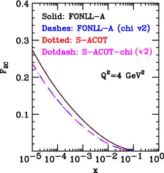
Figure 7: Comparison of $F_{2}^{c}$ for the Fixed-Order-Next-to-Leading-Log (FONLL) with the Simplified-ACOT (S-ACOT) scheme. There are four curves displayed, two for the ordinary $\chi$-rescaling, and two for an alternate $\chi$-rescaling (labeled “v2”). The FONLL and S-ACOT results are identical throughout the $x$ range. (Figure from Ref. [22].)

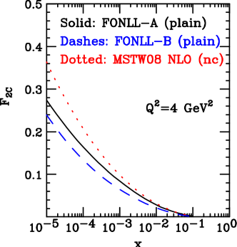
Figure 8: Comparison of $F_{2}^{c}$ for the Fixed-Order-Next-to-Leading-Log (FONLL) and the MSTW08 NLO results. The FONLL results are shown for both the “A” and “B” variations. The FONLL results differ from the MSTW08 results for low $Q$ and $x$; for larger values of $Q$ and $x$ they are more comparable. (Figure from Ref. [22].)

Having illustrated the impact of different theoretical schemes on the data analysis, we take a moment to compare and contrast some of the different schemes that are currently being used for various PDF analysis efforts. While many of the global analyses use a Variable Flavor Number (VFN) scheme to include the heavy quark as a parton, the detailed implementation of this scheme can lead to notable differences. At the 2009 Les Houches workshop, a comparison was performed among a number of the different programs to quantify these differences. All programs used the same PDFs and $\alpha_{S}$ values so that the differences would only reflect the particular scheme. The complete details can be found in Ref. [22], and Figures 7 and 8 display sample comparisons.

Figure 7 compares the S-ACOT scheme which is used for the CTEQ series of global analyses, [23, 24] and the FONLL which is used by the Neural Network PDF (NNPDF) collaboration. [25] In the figure, these two implementations (S-ACOT and FONLL-A) are numerically equivalent.

Figure 8 compares two variations of the FONLL scheme (“A” and “B”) with the MSTW08 results which is used in the MSTW series of PDF global analyses. [26, 27] Here these differences reflect the different organization and truncation of the perturbation expansion; it does not indicate that one choice is right or wrong. We expect such differences to be proportional to $\sim\alpha_{S}^{N}\times{\cal O}(m^{2}/Q^{2})$. Thus, as we increase the order of perturbation theory or the energy scale the differences should decrease; we have explicitly verified the difference is reduced as $Q^{2}$ increases, as it should. When we are able to carry these calculations out to higher orders, the scheme differences should be further reduced; this work is in progress.

Charm Mass Dependence and $F_{2}^{c}$

The experimental extraction of the “inclusive” $F_{2}^{c}$ requires a differential NLO calculation of DIS charm production to be extrapolated over the unobserved kinematic regions. These analyses generally make use of the HVQDIS program [28] which computes $F_{2}^{c}$ in a Fixed-Flavor-Number (FFN) scheme at NLO. In this calculation, the charm is produced only via a gluon splitting, $g\to c\bar{c}$, and there is no charm PDF. Thus, the charm mass ($m_{c}$) enters only the partonic cross section $\hat{\sigma}(m_{c})$ and the final state phase space; there is no PDF charm threshold.

Although we would also like to perform the extraction of $F_{2}^{c}$ using a Variable-Flavor-Number (VFN) scheme, the challenge is that no NLO differential program exists for this process. In lieu of a VFN extraction, another avenue is to study the influence of different theoretical schemes and $m_{c}$ parameters in the analysis of the $F_{2}^{c}$ data. We describe such a study below.

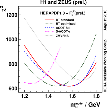
Figure 9: Comparison of $\chi^{2}$ for HERA I + $F_{2}^{c\bar{c}}$ fits using different heavy flavor schemes as a function of the charm quark mass parameter $m_{c}^{model}$. (Figure from H1prelim-10-143 & ZEUS-prel-10-019)

In many analyses, the value of the charm mass is taken as an external fixed parameter. A recent investigation has taken a closer look at the role of the charm mass parameter $m_{c}$ and examined the combined effects of $m_{c}$ and the theoretical scheme used; preliminary results of this study are displayed in Figure 9. For each of the schemes listed in the legend, fits were generated for fixed $m_{c}$ values in the range $[1.2,1.8]$ GeV. Thus, the minimum of the $\chi^{2}$ curve represents the “optimal” choice of the charm mass parameter $m_{c}$ for that specific scheme.

We observe that the various schemes prefer $m_{c}$ values ranging from 1.2 to 1.7 GeV, The largest $m_{c}$ value (1.68 GeV) comes from the Zero Mass VFN Scheme (ZM  VFNS) which only uses $m_{c}$ for the PDF charm threshold; it is absent in the phase space for the zero-mass case. In contrast, for the S-ACOT-$\chi$ scheme the “$\chi$” notation indicates there are effectively two factors of $m_{c}$ in the final phase space, and this yields the smallest value of $m_{c}$ (1.26 GeV).

The ACOT scheme and the Roberts-Thorne (RT) scheme yield $m_{c}$ values in the intermediate region. The ACOT scheme uses the full kinematic mass relations in the partonic relations, and the scaling variable is intermediate ($m_{c}$=1.58 GeV) between the ZM-VFN scheme and the S-ACOT-$\chi$ scheme. The S-ACOT scheme (not shown) is virtually identical to the full ACOT scheme, and also yields a $m_{c}$ value in the intermediate region. Therefore, comparing the S-ACOT-$\chi$ and S-ACOT schemes, we find that the $\chi$-rescaling variable is dominantly responsible for the shift of the optimal $m_{c}$ value from $\sim 1.26$ to $\sim 1.58$. This observation suggests that it is the rescaling of the $x$ variable which enters the PDFs that generates the dominant effect. While this study is continuing, it does indicate the sensitivity of the charm mass and scheme choice in these precision analyses.

Extrinsic & Intrinsic Charm PDFs

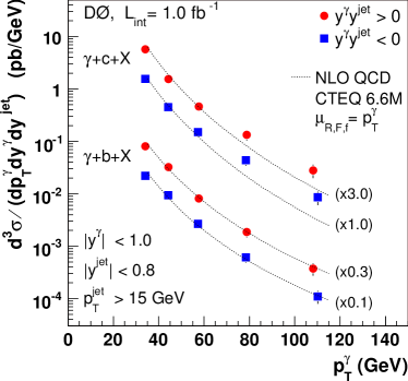
Figure 10: Measurement of $\gamma+c$ and $\gamma+b$ vs. $P_{T}^{\gamma}$ as measured by D-Zero. (Figure from Ref. [32].)

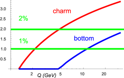
Figure 11: The integrated momentum fraction (in percent) of the “extrinsic” charm and bottom quarks generated by gluon splitting as a function of the scale $Q$. Reference lines are indicated at 1% and 2%.

Figure 12: $d\sigma/dp_{T\gamma}$ (pb/GeV) at the Tevatron for the CTEQ6.6 PDFs, and two intrinsic charm (IC) models. (Figure from Ref. [30].)

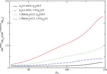
Figure 13: Ratio of $d\sigma/dp_{T\gamma}$ (pb/GeV) at the LHC ($\sqrt{s}=7~{}TeV$) for the BPHS IC model to the CTEQ6.6 PDF for a selection of rapidity bins. (Figure from Ref. [30].)

The charm quark and bottom quark PDFs can be probed directly at the Tevatron by studying photon–heavy quark final states which occur via the sub-process $gQ\to\gamma Q$ at LO. This process has been measured at the Tevatron for both charm and bottom final states, and we display the results in Figure 10 as a function of $P_{T}^{\gamma}$ for two rapidity configurations. This measurement is particularly interesting as the dominant process involves a heavy quark PDF; this is in contrast to DIS charm or bottom production, for example, where over much of the kinematic range the process is dominated by the gluon-initiated process (e.g., $\gamma g\to Q\bar{Q}$) rather than the heavy quark initiated process ($\gamma Q\to Q$).

Examining Figure 10 we observe that the bottom quark production measurements compare favorably with the theoretical predictions throughout the $P_{T}^{\gamma}$ range, but the charm results rise above the theory predictions for large $P_{T}^{\gamma}$. Although there may be a number of explanations for the excess charm cross section at large $P_{T}^{\gamma}$, one possibility is the presence of intrinsic charm (IC) in the proton. In the usual DGLAP evolution of the proton PDFs, we begin the evolution at a low energy scale $Q_{0}<m_{c}$ and evolve up to higher scales. The charm and bottom PDFs are defined to be zero for $Q<m_{c,b}$, and above the mass scale the heavy quark PDFs are generated by gluon splitting, $g\to Q\bar{Q}$; we refer to this as the “extrinsic” contribution to the heavy quark PDFs. In Figure 11 we display the integrated momentum fractions for the charm and bottom quarks as a function of the scale $Q$; these are zero for $Q<m_{c,b}$, and then begin to grow via the $g\to Q\bar{Q}$ process.

It has been suggested that there may also be an “intrinsic contribution to the heavy quark PDFs which is present even at low scales $Q<m_{c,b}$. While it is difficult to constrain the detailed functional shape of any intrinsic heavy quark distribution, the total momentum fraction of any intrinsic contribution must be less than approximately $1\%$ if it is to be compatible with the global analyses.

In Figure 12 we illustrate the effect of including an additional intrinsic charm component in the proton. The BHPS IC model concentrates the momentum fraction at large $x$ values, and the Sea-like IC model distributes the charm more uniformly. It is intriguing that the IC modification of the proton PDF can increase the theoretical prediction in the large $P_{T}^{\gamma}$ region, but this observation alone is not sufficient to claim the presence of IC; this would require independent verification. In Figure 13 we display the cross section ratio for $\gamma+c$ at the LHC for the BHPS IC model for a selection of rapidity bins. Thus the LHC can validate or refute this possibility with a high-statistics measurement of $\gamma+c$, especially if they can observe this in the forward rapidity region.

The Longitudinal Structure Function $F_{L}$

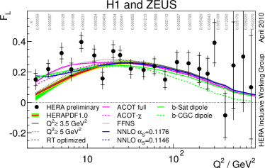
Figure 14: Measurement of $F_{L}$ using the combined HERA data set from H1 and ZEUS. The data are compared with a selection of theoretical predictions. (Figure H1prelim-10-044 & ZEUS-prel-10-008).

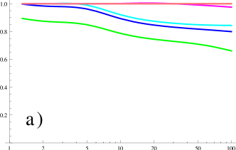
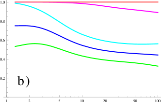
Figure 15: Fractional flavor decomposition of $F_{L}^{i}/F_{L}$ vs. $Q$ in GeV for a) $x=10^{-1}$ and b) $x=10^{-5}$. Reading from the bottom, we plot the cumulative contributions for $\{u,d,s,c,b\}$.

Most of the previous discussion has addressed the determination of the quark PDFs. Constraining the gluon PDF is a challenge, and the longitudinal structure function $F_{L}$ is particularly interesting as it involves both the heavy quark and the gluon distributions. Using the combined data from H1 and ZEUS, HERA has extracted $F_{L}$ in an extended kinematic regime, and Figure 14 displays the result of the combined data as compared with various theoretical predictions.

The measurement of $F_{L}$ is special for a number of reasons, and we write this schematically as:

$$F_{L}\simeq\frac{m^{2}}{Q^{2}}\ q(x)+\alpha_{S}\left\{C_{g}\otimes g(x)+C_{q}\otimes q(x)\right\}\ .$$ (1)

Note that the LO term is zero in the limit of massless quarks as the $(m^{2}/Q^{2})$ factor in Eq. (1) suppresses the helicity violating contributions; this is a consequence of the Callan-Gross relation. Therefore, for light quarks the dominant contributions come from the NLO gluon term; hence, $F_{L}$ can provide useful information about the gluon PDF.

For the heavy quarks the picture is less obvious. While the NLO heavy quark contributions will clearly be small compared to the dominant gluon terms, the heavy quarks can contribute at LO if they can overcome the $(m^{2}/Q^{2})$ suppression. This is why the prediction of $F_{L}$ into the low $Q^{2}$ region as measured in Figure 14 is such a theoretical challenge. This raises a number of questions: What is the flavor composition of $F_{L}$? Where are the heavy quark contributions important?

In Figure 15 we display the fractional contributions to the structure functions $F_{L}^{i}/F_{L}$ vs. $Q$. We observe that for large $x$ and low $Q$ the heavy flavor contributions are minimal. For example, in Figure 15-a) at $Q\sim$ 5 GeV we see the $u$-quark structure function $F_{L}^{u}$ comprises $\sim 80\%$ of the total, $F_{L}^{d}$ is about 10%, and the $s$, $c$ and $b$ quarks divide the remaining fraction.

At smaller $x$ values the picture changes and the heavy quarks are more prominent. In Figure 15-b) for $Q\sim 2~{}GeV$ we see the $u$-quark structure function $F_{L}^{u}$ comprises $\sim 55\%$, $F_{L}^{d}$ and $F_{L}^{s}$ are both about 20%, and the $c$ and $b$ quarks make up the small remaining fraction. However, $F_{L}^{c}$ increases quickly as $Q$ increases and is comparable to $F_{L}^{u}$ ($\sim 40\%$) for $Q\sim 20~{}GeV$. Additionally, for large $Q\sim 100~{}GeV$ we see the contributions of the $u$-quark and $c$-quark are comparable, the $d$-quark and $s$-quark are comparable, and the relative sizes of the $u,c$  to $d,s$  terms are proportional to their couplings: 4/9 to 1/9. Thus, for low $x$ and intermediate to large $Q$ values we see that the quark masses (aside from the top) no longer play a prominent role and we approach the limit of “flavor democracy.”

Concluding Remarks

We reviewed a number of recent developments regarding the extraction and application of heavy quark Parton Distribution Functions (PDFs). The high precision HERA measurements were essential in developing and refining the theoretical treatment of the heavy quarks. Even though the accelerator facility stopped operation four years ago, the analysis of the data continues. The results of these analyses will provide the foundation upon which future PDF analyses will be built, and the advances of the experimental analysis and theoretical tools developed at HERA will continue to influence future hadronic studies including those now beginning at the LHC.

Acknowledgment

We thank M. Botje, A. M. Cooper-Sarkar, A. Glazov, C. Keppel, J. G. Morfín, P. Nadolsky, J. F. Owens, V. A. Radescu, and M. Tzanov for valuable discussions, and we acknowledge the hospitality of CERN, DESY, Fermilab, and Les Houches where a portion of this work was performed. F.I.O thanks the Galileo Galilei Institute for Theoretical Physics for their hospitality and the INFN for partial support during the completion of this work. This work was partially supported by the U.S. Department of Energy under grant DE-FG02-04ER41299, and the Lightner-Sams Foundation. The work of J. Y. Yu was supported by the Deutsche Forschungsgemeinschaft (DFG) through grant No. YU 118/1-1. The work of K. Kovařík was supported by the ANR projects ANR-06-JCJC-0038-01 and ToolsDMColl, BLAN07-2-194882. F.I.O. is grateful to DESY Hamburg and MPI Munich for their organization and support of the Ringberg Workshop.

References

- [1] K. Kovarik, I. Schienbein, F. Olness, J. Yu, C. Keppel, et al., Nuclear corrections in neutrino-nucleus DIS and their compatibility with global NPDF analyses, Phys.Rev.Lett. 106 (2011) 122301. arXiv:1012.0286, doi:10.1103/PhysRevLett.106.122301.
- [2] I. Schienbein, et al., Nuclear PDFs from neutrino deep inelastic scattering, Phys. Rev. D77 (2008) 054013. arXiv:0710.4897, doi:10.1103/PhysRevD.77.054013.
- [3] S. A. Kulagin, R. Petti, Global study of nuclear structure functions, Nucl. Phys. A765 (2006) 126–187. arXiv:hep-ph/0412425, doi:10.1016/j.nuclphysa.2005.10.011.
- [4] S. A. Kulagin, R. Petti, Neutrino inelastic scattering off nuclei, Phys. Rev. D76 (2007) 094023. arXiv:hep-ph/0703033, doi:10.1103/PhysRevD.76.094023.
- [5] M. Hirai, S. Kumano, T. H. Nagai, Determination of nuclear parton distribution functions and their uncertainties at next-to-leading order, Phys. Rev. C76 (2007) 065207. arXiv:0709.3038, doi:10.1103/PhysRevC.76.065207.
- [6] A. Bodek, et al., Electron Scattering from Nuclear Targets and Quark Distributions in Nuclei, Phys. Rev. Lett. 50 (1983) 1431. doi:10.1103/PhysRevLett.50.1431.
- [7] G. Bari, et al., A Measurement of Nuclear Effects in Deep Inelastic Muon Scattering on Deuterium, Nitrogen and Iron Targets, Phys. Lett. B163 (1985) 282. doi:10.1016/0370-2693(85)90238-2.
- [8] A. C. Benvenuti, et al., Nuclear Effects in Deep Inelastic Muon Scattering on Deuterium and Iron Targets, Phys. Lett. B189 (1987) 483. doi:10.1016/0370-2693(87)90664-2.
- [9] U. Landgraf, Nuclear effects in deep inelastic scattering, Nucl. Phys. A527 (1991) 123c–135c. doi:10.1016/0375-9474(91)90110-R.
- [10] J. Gomez, et al., Measurement of the A-dependence of deep inelastic electron scattering, Phys. Rev. D49 (1994) 4348–4372. doi:10.1103/PhysRevD.49.4348.
- [11] S. Dasu, et al., Measurement of kinematic and nuclear dependence of in deep inelastic electron scattering, Phys. Rev. D49 (1994) 5641–5670. doi:10.1103/PhysRevD.49.5641.
- [12] E. Rondio, Nuclear effects in deep inelastic scattering, Nucl. Phys. A553 (1993) 615c–624c. doi:10.1016/0375-9474(93)90668-N.
- [13] M. Tzanov, et al., Precise measurement of neutrino and anti-neutrino differential cross sections, Phys. Rev. D74 (2006) 012008. arXiv:hep-ex/0509010, doi:10.1103/PhysRevD.74.012008.
- [14] J. Botts, et al., CTEQ parton distributions and flavor dependence of sea quarks, Phys. Lett. B304 (1993) 159–166. arXiv:hep-ph/9303255, doi:10.1016/0370-2693(93)91416-K.
- [15] H. L. Lai, et al., Global QCD analysis and the CTEQ parton distributions, Phys. Rev. D51 (1995) 4763–4782. arXiv:hep-ph/9410404, doi:10.1103/PhysRevD.51.4763.
- [16] I. Schienbein, J. Yu, K. Kovarik, C. Keppel, J. Morfin, et al., PDF Nuclear Corrections for Charged and Neutral Current Processes, Phys.Rev. D80 (2009) 094004. arXiv:0907.2357, doi:10.1103/PhysRevD.80.094004.
- [17] F. D. Aaron, et al., Measurement of Meson Production and Determination of at low in Deep-Inelastic Scattering at HERA, Eur. Phys. J. C71 (2011) 1769. arXiv:1106.1028, doi:10.1140/epjc/s10052-011-1769-0.
- [18] S. Chekanov, et al., Measurement of charm and beauty production in deep inelastic ep scattering from decays into muons at HERA, Eur. Phys. J. C65 (2010) 65–79. arXiv:0904.3487, doi:10.1140/epjc/s10052-009-1193-x.
- [19] J. Breitweg, et al., Measurement of production and the charm contribution to in deep inelastic scattering at HERA, Eur. Phys. J. C12 (2000) 35–52. arXiv:hep-ex/9908012, doi:10.1007/s100529900244.
- [20] C. Adloff, et al., Measurement of meson production and in deep inelastic scattering at HERA, Phys. Lett. B528 (2002) 199–214. arXiv:hep-ex/0108039, doi:10.1016/S0370-2693(02)01195-4.
- [21] S. Kretzer, H. L. Lai, F. I. Olness, W. K. Tung, CTEQ6 parton distributions with heavy quark mass effects, Phys. Rev. D69 (2004) 114005. arXiv:hep-ph/0307022, doi:10.1103/PhysRevD.69.114005.
- [22] J. R. Andersen, et al., The SM and NLO multileg working group: Summary reportarXiv:1003.1241.
- [23] H.-L. Lai, M. Guzzi, J. Huston, Z. Li, P. M. Nadolsky, et al., New parton distributions for collider physics, Phys.Rev. D82 (2010) 074024. arXiv:1007.2241, doi:10.1103/PhysRevD.82.074024.
- [24] P. M. Nadolsky, H.-L. Lai, Q.-H. Cao, J. Huston, J. Pumplin, et al., Implications of CTEQ global analysis for collider observables, Phys.Rev. D78 (2008) 013004. arXiv:0802.0007, doi:10.1103/PhysRevD.78.013004.
- [25] R. D. Ball, et al., Unbiased global determination of parton distributions and their uncertainties at NNLO and at LO, Nucl.Phys. B855 (2012) 153–221. arXiv:1107.2652, doi:10.1016/j.nuclphysb.2011.09.024.
- [26] A. Martin, W. Stirling, R. Thorne, G. Watt, Heavy-quark mass dependence in global PDF analyses and 3- and 4-flavour parton distributions, Eur.Phys.J. C70 (2010) 51–72. arXiv:1007.2624, doi:10.1140/epjc/s10052-010-1462-8.
- [27] A. Martin, W. Stirling, R. Thorne, G. Watt, Parton distributions for the LHC, Eur.Phys.J. C63 (2009) 189–285. arXiv:0901.0002, doi:10.1140/epjc/s10052-009-1072-5.
- [28] B. W. Harris, J. Smith, Charm quark and cross sections in deeply inelastic scattering at HERA, Phys. Rev. D57 (1998) 2806–2812. arXiv:hep-ph/9706334, doi:10.1103/PhysRevD.57.2806.
- [29] R. Barnett, Evidence for New Quarks and New Currents, Phys.Rev.Lett. 36 (1976) 1163–1166. doi:10.1103/PhysRevLett.36.1163.
- [30] T. Stavreva, Heavy quark & direct photon production and heavy quark parton densities, Nucl.Phys.Proc.Suppl. 214 (2011) 114–117. arXiv:1012.1505, doi:10.1016/j.nuclphysbps.2011.03.069.
- [31] T. Stavreva, Direct Photon and Heavy Quark Jet Production at the LHC, PoS ICHEP2010 (2010) 360. arXiv:1012.1544.
- [32] V. Abazov, et al., Measurement of and production cross sections in p anti-p collisions at = 1.96-TeV., Phys.Rev.Lett. 102 (2009) 192002. arXiv:0901.0739, doi:10.1103/PhysRevLett.102.192002.