Radiation and Relaxation of Oscillons

Abstract

We study oscillons, extremely long-lived localized oscillations of a scalar field, with three different potentials: quartic , sine-Gordon model and in a new class of convex potentials. We use an absorbing boundary at the end of the lattice to remove emitted radiation. The energy and the frequency of an oscillon evolve in time and are well fitted by a constant component and a decaying, radiative part obeying a power law as a function time. The power spectra of the emitted radiation show several distinct frequency peaks where oscillons release energy. In two dimensions, and with suitable initial conditions, oscillons do not decay within the range of the simulations, which in quartic theory reach $10^{8}$ time units. While it is known that oscillons in three-dimensional quartic theory and sine-Gordon model decay relatively quickly, we observe a surprising persistence of the oscillons in the convex potential with no sign of demise up to $10^{7}$ time units. This leads us to speculate that an oscillon in such a potential could actually live infinitely long both in two and three dimensions.

I Introduction

The theorem by Derrick states that there are no non-trivial static solutions of finite energy in scalar theories above one dimension Derrick (1964). This does not say anything about time-dependent solutions. Example of such are Q-balls Coleman (1985), whose stability is guaranteed by a conservation law (for more recent studies on Q-balls see e.g. Multamaki and Vilja (2000); Tsumagari et al. (2008)) and that have been studied e.g. as a dark matter candidate (see for instance Dine and Kusenko (2004)). There is, however, no obvious reason why oscillations of a real scalar field can persist and stay localised, yet such configurations, oscillons exist in many models (we will use the term oscillon, presented originally in Gleiser (1994), in a slightly loose manner throughout this study). There is a stable breather solution in one-dimensional sine-Gordon model that during its period deforms to a separated kink and anti-kink. There is no such exactly stable solution in $\phi^{4}$ theory Segur and Kruskal (1987). However, even though the solution radiates energy away, there remains a possibility that the radiation rate is so suppressed that it will take indefinitely long for the dissipation to complete.

Oscillons were first found already in the 70’s Bogolyubsky and Makhankov (1976, 1977) and then rediscovered in the 90’s when the dynamics of phase transitions was studied Gleiser (1994). There has been substantial interest in oscillons recently. On the theoretical side of understanding the dynamics of oscillons, there have been a number of studies of oscillons of $\phi^{4}$ theory in small-amplitude approximation Fodor et al. (2006, 2008, 2009a, 2009b). Furthermore, the attractor basin of oscillons and its fractal nature have been studied both analytically Di Plinio et al. (2010) and numerically Honda (2010). Very recently there has been interest in oscillons coupled to gravity, oscillatons Fodor et al. (2010); Grandclement et al. (2011); Valdez-Alvarado et al. (2011). Oscillons have also been found in dilaton-scalar theories Fodor et al. (2009c). A new class of solutions, called flat-top oscillons by the authors, were reported in Amin and Shirokoff (2010). While the body of work mentioned above has been on a classical level, the study in Hertzberg (2010) considered quantum corrections oscillons are subject to, redeeming oscillons considerably less robust against the quantum effects than often previously has been assumed.

Though stability or finite lifetime are of considerable theoretical interest, from the point of view of a many phenomenological consequences, it is not important if the non-trivial solutions are actually stable like the breather in one-dimensional sine-Gordon model as long as they are far longer-lived than the natural time scale related to the process on which they will have an effect. A natural realm of oscillons to appear is in the early Universe and such a process there could be baryogenesis. The role oscillons could potentially have on baryogenesis is providing the necessary non-equilibrium needed for successful creation of matter-antimatter asymmetry analogous to Q-balls whose cosmological impact has been studied extensively (for a review, see e.g. Enqvist and Mazumdar (2003)). In this context it is very interesting that an oscillon solution has been found in the bosonic sector of the Standard Model  Farhi et al. (2005); Graham (2007a, b). When the scalar and vector masses in the theory are set to be $m_{H}=2m_{W}$, the oscillon is sufficiently long-lived that it has not been seen to decay in any numerical simulation to date Farhi et al. (2005); Graham (2007a, b). Oscillons have also been found in two and three-dimensional Abelian-Higgs model in deep type I regime Gleiser and Thorarinson (2007, 2009). A number of studies have considered oscillons in the early Universe. While the oscillons in the Standard Model or Abelian-Higgs model are obviously objects in several fields, a recent study Gleiser et al. (2011) found that oscillons can also form in two scalar fields in models that are relevant from the point of view of hybrid inflation (on that topic see also Broadhead and McDonald (2005)). Other recent studies of formation of oscillons after an inflationary epoch but in single field models include Amin et al. (2010, 2011a). Regarding the subsequent evolution of oscillons after their formation in a cosmological setting, both numerical Graham and Stamatopoulos (2006) and analytical Farhi et al. (2008) considerations in one dimension have shown that oscillons can persist for a considerably time in expanding backgrounds (see also Amin and Shirokoff (2010)). The proposal of oscillons facilitating vacuum tunneling in the context of the string landscape Saffin et al. (2008) is an application quite far from the original idea of oscillons affecting the bubble nucleation process, the resonant nucleation studied e.g. in Gleiser and Howell (2005) (for a study of bubble collisions, see also Dymnikova et al. (2000)). A recent study considered the formation of oscillons in the quintessence field at the present epoch of the Universe Amin et al. (2011b).

Lastly, regarding the significance of the oscillons, it should be mentioned that they are an interesting link between particles and solitons. Several numerical studies in one dimension have considered the formation of kink-antikink pairs. It has been found that scattering of breathers can create a kink and an antikink Dutta et al. (2008). Oscillons can also decay to a kink and antikink when the potential of the model is distorted Carvalho and Perivolaropoulos (2009), as well as oscillons being an intermediate state in the process of formation of the kink-antikink pair Romanczukiewicz and Shnir (2010).

In an earlier work Hindmarsh and Salmi (2006) we studied oscillons in two dimensions on the lattice with periodic boundary conditions. The aim of this study is to examine in detail the evolution of oscillons and the properties of the radiation they emit, in order to better understand the reasons for their longevity with the use of absorbing boundary conditions.

Previous work in a theory with a quartic potential has identified stable periodic solutions with incoming radiation, called quasl-breathers, which are closely related to oscillons Watkins (1996); Saffin and Tranberg (2007). There is a critical oscillation frequency at which the quasi-breather has the minimum energy Watkins (1996); Saffin and Tranberg (2007), and once the incoming radiation is removed, the frequency of the resulting solution evolves towards its critical value according to a power law in time Saffin and Tranberg (2007). Power laws featured also strongly in Gleiser and Sicilia (2008, 2009) where the radiation rates of oscillons were studied, starting from the assumption of a strictly Gaussian form for the oscillon, and a decay width calculated by comparison to linear theory. An equation relating the energy loss rate to the rate of change of the oscillon amplitude was derived, with power law solutions for the time evolution. Note that oscillons in the small-amplitude expansion Fodor et al. (2009a, b) behave differently, in that they shed energy in an exponentially suppressed way as the amplitude goes to zero, and do not obey a simple power law.

model	potential $V(\phi)$
quartic ($\phi^{4}$)	$\displaystyle\frac{1}{4}(\phi^{2}-1)^{2}$
sine-Gordon	$\displaystyle\frac{1}{\pi^{2}}(1+\cos(\pi\phi))$
convex	$\displaystyle\frac{\phi^{2}}{1+\phi^{2p}}$

Table 1: Potentials for the three models considered in this paper. In the convex potential, $p$ is a real parameter, with $p<1$. For the data shown $p=0.45$.

In this paper we determine these power laws in three models in two and three dimensions, consisting of a single canonically normalised real scalar field $\phi$ with potentials listed in Table 1, and examine the power spectra of the emitted radiation. Our power spectra show that for the quartic and sine-Gordon theories the radiation is predominantly emitted at an integer multiple of the basic oscillation frequency, either 3 or 2 depending whether the potential is symmetric or not. For the convex potential, the radiation is emitted just above the threshold set by the mass parameter. A fundamental assumption made in Gleiser and Sicilia (2009) in developing a theory of oscillons in the quartic theory was that the radiation is predominantly emitted just above threshold, which we see is incorrect. Nonetheless, good fits to the time evolution of the energy, frequency and amplitude were obtained in that work.

An important technical development in our work is the construction of absorbing boundary conditions for a massive field, which provides an economical alternative to the adiabatic damping technique, introduced in Gleiser and Sornborger (2000), and also used in Saffin and Tranberg (2007), which sets a location dependent friction co-efficient on the lattice. Absorbing boundaries provide an alternative approach to remove the dispersive waves from the lattice, requiring no extra lattice sites for its operation.

The paper is organised as follows. The numerical set-up is briefly reviewed in the following section. While the equations of the absorbing boundary conditions are presented in the appendix we briefly discuss their implications for simulations together with the data obtained using quartic theory as an example. We then proceed to present the results for the power laws and the radiation power spectra in the three theories in two and three dimensions. We find a surprising stability for the oscillon in the convex potential, which leads us to conjecture that it may be stable in three dimensions.

II Numerical Set-up

The Lagrangian for a single real scalar field $\phi$ is given by

$$\mathscr{L}=\frac{1}{2}{\partial}_{\mu}\phi{\partial}^{\mu}\phi-V(\phi),$$ (1)

and the equation of motion thus reads

$$\ddot{\phi}-\nabla^{2}\phi+V^{\prime}(\phi)=0.$$ (2)

This field equation is evolved using a leapfrog update and a three-point spatial Laplacian accurate to O($dx^{2}$). We perform (1+1)-dimensional simulations assuming radial symmetry. These permit the choice of a much finer lattice spacing compared with (2+1)-dimensional simulations carried out in a previous study Hindmarsh and Salmi (2006). We kept the ratio of time step and lattice spacing fixed and matching to the one used in (2+1)-dimensional simulations, $dt:dx=1:5$. The size of the one-dimensional grid was chosen so that the physical distance from the core of the oscillon to the absorbing boundary was always $100$ units. The simulations are performed on a grid of 10,001 lattice points and $dx=0.01$, $dt=0.002$.

We set the field $\phi$ and the field momentum $\Pi=\dot{\phi}$ at the origin $r=0$ to have the same value as on the next lattice site with a non-zero value of the radius $r$. The updates used at the far end of the grid, where the absorbing boundary is located, are derived in the appendix, while we comment the simulations with the absorbing boundaries shortly in the next section. We use three consecutive points in the grid to evaluate the gradients with the precision also accurate to O($dx^{2}$).

III Quartic Potential

We study here the degenerate double-well quartic potential which defines the model that we refer also as $\phi^{4}$ theory

$$V(\phi)=\frac{1}{4}\lambda(\phi^{2}-v^{2})^{2}\,,$$ (3)

which sets the mass of the theory to be $m^{2}=2\lambda v^{2}$. Scaling out the vacuum expectation value and coupling the potential can be written

$$V(\phi)=\frac{1}{4}(\phi^{2}-1)^{2}$$ (4)

so that the minima are located at $\phi=\pm 1$ and the local maximum at $\phi=0$. We use the following Gaussian initial data to create an oscillon

$$\phi(r)=\,\left(1-C\cdot\exp(-r^{2}/r_{0}^{2})\right),$$ (5)

where $r$ is the distance to the center of an oscillon. The width of the distribution is set to be $r_{0}\simeq 2.9$ (in units of $(\sqrt{\lambda}\,\eta)^{-1}$) in two and $r_{0}\simeq 3.0$ in three dimensions, suggested optimal choices in Copeland et al. (1995). The maximum displacement in two dimensions is set to be $C=1$ so that the center of the oscillon starts from the local maximum of the potential, while we use $C=-1$ in three dimensions again following Copeland et al. (1995).

III.1 Properties in $\phi^{4}$ theory in two dimensions

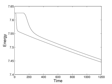
Figure 1: The total energy in the lattice (top) and energy inside a shell of radius $r=5r_{0}$ (bottom) in $\phi^{4}$ theory in two dimensions.

As we kick off the oscillon by the somewhat arbitrary initial condition (5), it naturally sheds at least some fraction of the energy in the form of propagating waves moving away. As long as that emission is not too violent and at least further distance away from the oscillon core spreading and consequently damped in two or higher dimensions these waves can be assumed to be well-characterized just by a linear approximation of the equation of motion (2), see (13). Once the wave reaches the boundary of the grid it is absorbed and the energy carried by the wave removed from the lattice. We thus expect monotonically decreasing total energy in the system, and this is also what we observe. Figure 1 shows the total energy (top line) in the lattice at the very early stage of the simulation. The total energy in the lattice will always include the radiative component emitted by the oscillon which has not yet reached the boundary of the grid. Thus we measure also the energy inside the radius $r=5r_{0}$ from the center of the oscillon and refer this as the energy of the oscillon. The oscillon is generally well localised inside this volume, but it covers less than $15\%$ of the lattice used here. The energy inside this shell is also depicted in Figure 1 (bottom line). In the beginning it takes a finite time the wave to reach the boundary and even then the decrease in total energy is more gradual compared with the energy inside the shell; this is caused by the dispersion of the emitted waves. However, after the initial transient phase these two ways to measure energy track each other well; there is only a time delay between them. This also provides a crucial check for the adequacy of the absorbing boundary conditions we use. Any reflected waves will travel back and reach the inner shell consequently increasing energy measured inside the radius there. There is no sign of such a burst at a visible level in Figure 1 and we expect only a very minor reflection taking place at the boundary. We monitor the total energy and the energy inside the aforementioned shell throughout the simulations.

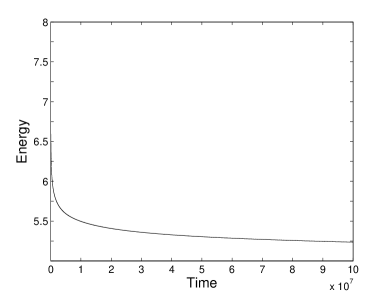
Figure 2: The energy inside a shell of radius $r=5r_{0}$ in $\phi^{4}$ theory in two dimensions over the span of the simulation up to $10^{8}$ time units.

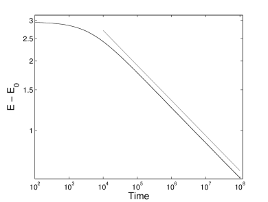
Figure 3: The difference of the energy inside a shell of radius $r=5r_{0}$ and the constant $E_{0}=4.613$ in $\phi^{4}$ theory in two dimensions. The grey straight line is a guide to eye of a power law $(E-E_{0})\sim t^{-\delta}$ with the slope $\delta=0.152$.

While at the early stage there is seemingly linear decrease in energy of the oscillon as shown in Figure 1, this rate of energy loss flattens out. Figure 2 shows the energy inside the radius $r=5r_{0}$ over the simulation that reaches over $10^{8}$ time units. First of all, there is no sign of the demise of the oscillon by this point in time. The energy is naturally monotonically decreasing function of time, but the rate of decrease slows down raising the question if the energy approaches asymptotically a constant value, which we denote by $E_{0}$ from now on. We searched for a power law of the form $\left(E(t)-E_{0}\right)\sim t^{-\delta}$. In practice we performed least-square fit with three free parameters, the asymptotic energy $E_{0}$, the exponent $\delta$ and an amplitude in the power law for the data. The best fit for the data presented in Figure 2 is shown in Figure 3 where we plot the difference of the energy inside the shell and the constant $E_{0}=4.613$ on a logarithmic scale. The grey line is a guide to eye of a slope $-0.152$. There is very good agreement to this over three orders of magnitude in time providing strong evidence for the power law decay of the radiative component governed by a small exponent $\delta=0.1520\pm 0.0005$ (we quote hereafter uncertainties in quantities based on $68\%$ confidence intervals derived from standard regression analysis applied to the subset of the data used for the fit). Moreover, there exist asymptotic value for the energy $E_{0}$ of the oscillon with a value $E_{0}=4.613\pm 0.003$, thus $E_{0}\gtrsim 4.6$.

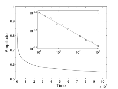
Figure 4: The amplitude as a function of time in $\phi^{4}$ theory in two dimensions. The inset shows the data points in the fit $A-A_{0}$ for $A_{0}=0.33$ for time greater than $10^{5}$. The grey straight line is the best fit power law $(A-A_{0})\sim t^{-\varrho}$ with the slope $\varrho=0.13$.

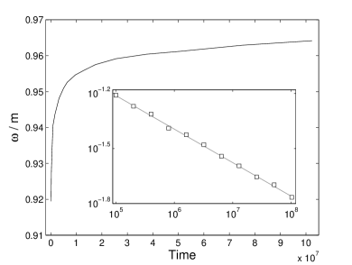
Figure 5: The oscillation frequency as a function of time in $\phi^{4}$ theory in two dimensions. The inset shows the data points in the fit $\omega^{\star}-\omega$ for $\omega^{\star}=0.981$ for time greater than $10^{5}$. The grey straight line is the best fit power law $(\omega^{\star}-\omega_{0})\sim t^{-\gamma}$ with the slope $\gamma=0.182$.

The decrease in energy is a consequence of the decline in the amplitude of the oscillations, i.e. the maximum excursion the field makes at the center of the oscillon, which we take to be towards the local maximum of the potential, initially set by $C=1$. The amplitude $A$ as a function of time is shown in Figure 4. Also this quantity is fitted relatively well by a power law, $\left(A(t)-A_{0}\right)\sim t^{-\varrho}$. The best-fit values for the asymptotic value of the amplitude is $A_{0}=0.33\pm 0.06$ and for the exponent governing the power law $\varrho=0.13\pm 0.02$. The comparison between the best-fit and the data is shown in the inset in Figure 4. This suggests that the oscillations would still undergo a substantial decrease in size before reaching the asymptotic value $A_{0}$. It should be noted that as the amplitude is not an integrated quantity like the energy of the oscillon, the uncertainty in the fit is prominently larger, and there remains scatter as can be seen in the inset in Figure 4.

With decreasing amplitude the frequency of the oscillon increases. We measure the frequency through the oscillation period, determined from the field’s three consecutive crossings of the minimum of the potential at the center of the oscillon. Based on the time step used we expect the accuracy in determining the frequency from the data to be around $0.001$. Figure 5 shows the frequency as a function of time over the simulation. At the end of the simulation the frequency is $\omega=0.964$, still considerably below the threshold for radiation, $\omega/m=1$.

Previous numerical studies of quasi- or pseudo-breathers have established that there exists a critical frequency $\omega^{\star}$ such that $\omega^{\star}<1$ and above which the oscillon disintegrates when the dimensionality in $\phi^{4}$ theory is more than two Watkins (1996); Saffin and Tranberg (2007). Furthermore, it has been suggested that the approach of the frequency towards its critical value is governed by a power law as $\left(\omega^{\star}-\omega(t)\right)\sim t^{-\gamma}$ in Saffin and Tranberg (2007). Thus we searched again a power law by performing the least-square fit to the data. The best fit yields the critical frequency $\omega^{\star}=0.981\pm 0.003$ and the exponent governing the power law $\gamma=0.18\pm 0.02$. The data points for $\omega^{\star}-\omega(t)$ are depicted in the inset of Figure 5. There remains a considerable scatter from the central value, the grey straight line that demonstrates the best-fit power law $t^{-\gamma}$, but there is evidence for a critical frequency $\omega^{\star}<1$.

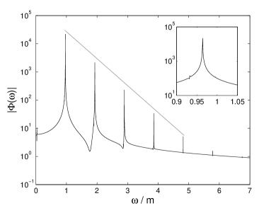
Figure 6: The power spectrum of the field at the center of the oscillon, $r=0$, in $\phi^{4}$ theory in two dimensions. The grey straight line is a guide to eye of the exponential $\exp(-b\,\omega)$ with the slope $b=2.2$. The inset shows the spectrum around the oscillation frequency $\omega_{0}\simeq 0.96$.

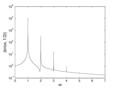
Figure 7: The Fourier transform of the Jacobi function ${\rm dn}(t,1/2)$. The height of the first peak is normalised to $10^{4}$ and its location to unity.

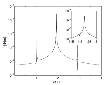
Figure 8: The power spectrum of the field far away from the oscillon core at $r=80$, in $\phi^{4}$ theory in two dimensions. The inset shows the spectrum around the location of the most prominent peak at $\omega\simeq 1.93$.

In addition to the oscillation frequency, the whole power spectrum of an oscillon is of interest and insight to the properties of oscillons can be gained by a study in frequency space. We denote the oscillation frequency now by $\omega_{0}$ to distinguish it from other frequencies present and secondly, to highlight that it can be considered a constant for any practical purposes in relatively short time intervals considered here. A separable ansatz consisting of a sum of multiplies of this frequency each with a separate spatial dependence has seen to converge quickly Watkins (1996); Honda and Choptuik (2002); Saffin and Tranberg (2007)

$$\phi(r,t)=\sum_{n=0}^{\infty}f_{n}(r)\cos(n\omega_{0}t)\,.$$ (6)

In an earlier work Hindmarsh and Salmi (2008) we used a method inspired by one-particle spectral function at zero momentum in classical approximation (for spectral function see Aarts and Smit (1998); Aarts (2001)). This technique, employed to trace oscillons moving with varying speed, could be utilised here as well. As the spectral function involves a volume average it produces generally quite a clean signal and reduces background noise. However, we wish to study the frequencies present at different locations on the grid and thus choose to obtain the straightforward Fourier transform of the field $\phi(r)$ on a fixed lattice site over a time interval.

Figure 6 shows the Fourier transform of the field at the center of the oscillon, $\phi(r=0)$ over the interval of length 5000 in time units starting at time $t=1.024\cdot 10^{8}$. The oscillation frequency $\omega_{0}$ (thus at this time $\omega_{0}=0.964$) is naturally the most pronounced mode, its multiples appearing in the spectra with starkly smaller amplitudes. This suppression is clearly exponential, illustrated by the grey straight line superimposed above the peaks in Figure 6. One should note here that when performing the discrete Fourier transform in a limited time interval it is likely that we do not capture the height of the very narrow peaks very precisely. The exponential fit to the data with the slope $-2.2$ should be thus considered rather indicative than quantitative. The results are qualitatively very similar to those obtained in Hindmarsh and Salmi (2006) where periodic boundary conditions were utilised in a two-dimensional lattice. However, the signal here is very clean; there is hardly any noise present, but the curve shown is a smooth line. We point out that fast Fourier transform of Jacobi functions in an interval yields a very similar signal, including the exponential suppression of the amplitudes at which the higher multiples of the basic frequency appear as well as similar patterns between the peaks. An example is given in Figure 7 where Jacobi function ${\rm dn}\left(\omega,1/2\right)$ is shown. The resemblance is not co-incidental - Jacobi functions are solutions to a type of elliptic non-linear differential equations that result also by omitting the spatial dependence in the equation of motion (2) in $\phi^{4}$ theory. Elliptic partial differential equations have also been shown to describe quasi-breathers in $\phi^{4}$ theory Fodor et al. (2008).

The use of absorbing boundary on the grid offers the oppourtunity to examine the outgoing radiation far away from the oscillon and circumvent the influence of the frequency directly related to oscillations at $\omega=\omega_{0}$. Figure 8 shows the Fourier transform of the field in the same time interval as in Figure 6, but at location $r=80$. This choice guarantees that the observation point is a considerable distance away from the oscillon core, but not at the edge of the lattice either where the equation of motion (2) is modified to create the absorbing boundary. There is signal at radiation frequency $\omega=1$ and just above it, but the most prominent peak is at the frequency $\omega\simeq 1.93$, thus coinciding with the second frequency $2\omega_{0}$ in the expansion (6). There is a peak in the spectra also at $3\omega_{0}$ and just a visible structure at $4\omega_{0}$, but the signal at $\omega=2\omega_{0}$ is the most dominant, the height of the peak being over thirty times larger than that at other frequencies, though still almost six orders of magnitude below the main peak at the oscillon core. This observation is evidence for that it is the first mode in (6) for which the frequency is above the radiation threshold (here $n=2$) that is primarily responsible for carrying away the energy from the oscillon.

III.2 Properties in $\phi^{4}$ theory in three dimensions

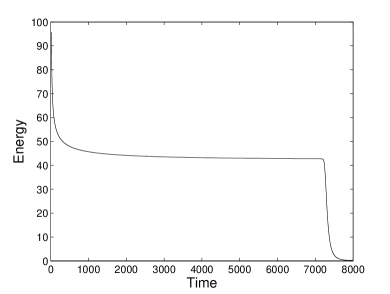
Figure 9: The energy inside a shell of radius $r=5r_{0}$ in $\phi^{4}$ theory in three dimensions.

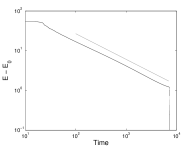
Figure 10: The difference of the energy inside a shell of radius $r=5r_{0}$ and the constant $41.56$ in $\phi^{4}$ theory in three dimensions. The grey straight line is a guide to eye of a power law given by $(E-E_{0})\sim t^{-\delta}$ with the slope $\delta=0.65$.

In three dimensions we start with a slightly broader width but considerably more energetic initial profile than in two dimensions as we set $C=-1$ and thus the amplitude of the excursion away from the minimum is towards the steeper side of the potential. The energy inside the radius $r=5r_{0}$ throughout the simulation is shown in Figure 9. There is a very abrupt drop in energy at the very beginning, but then the decrease slows down and energy stabilises above the value $E\approx 40$ for a considerable period of time, until the oscillon disintegrates around time $t=7200$ which appears in the data as the second stark drop in energy.

Even though the oscillon clearly has a finite lifetime here, the steady decrease in energy is relatively well captured by a power law. This is demonstrated in Figure 10 where the difference between the energy inside the shell and a constant $E_{0}=41.56$ is shown on a logarithmic scale. The best-fit value for the exponent is $\delta=0.65\pm 0.01$, thus the strength of the emitted radiation decays far faster in time than in two dimensions. This is naturally only of secondary importance because the asymptotic value for the energy $E_{0}=41.56\pm 0.05$ is well below the value when the oscillon destabilises, which is approximately at $E=42.7$.

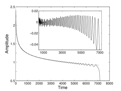
Figure 11: The amplitude as a function of time in $\phi^{4}$ theory in three dimensions. The grey line is a guide to eye of a power law given by $(A-A_{0})\sim t^{-\varrho}$ with $A_{0}=-1.374$ and $\varrho=0.066$. The inset shows the residuals in the afore mentioned fit.

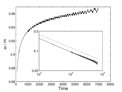
Figure 12: The oscillation frequency as a function of time in $\phi^{4}$ theory in three dimensions. The inset shows the data points in the fit $\omega^{\star}-\omega$ for $\omega^{\star}=1.030$ for time greater than $100$. The grey straight line is a guide to eye of a power law $(\omega^{\star}-\omega)\sim t^{-\gamma}$ with the slope $\gamma=0.2$.

The evolution of the amplitude $A$ of the oscillations is shown in Figure 11. On top of the general downward trend that follows closely the time evolution of the energy, the most notable feature is the growing fluctuation in this quantity in the course of time. This amplified oscillation in the amplitude around the central value with a decreasing frequency makes a simple power law fit to the data challenging. The best-fit to the data in the interval $500<{\rm time}<5000$ yields $A_{0}=-1.4\pm 0.3$ and $\varrho=0.066\pm 0.007$, but it should be emphasized that the values in the fit are very sensitive to the selection of the time interval. The residuals of the fit are shown on a linear scale in the inset in Figure 11. This highlights further the growing fluctuations, the beat, in the amplitude; to capture the time evolution of the amplitude entirely and adequately a model with extra parameters to account for these oscillations would be required. The negative value of the asymptotic amplitude $A_{0}$ indicates strongly the finite lifetime of the oscillon.

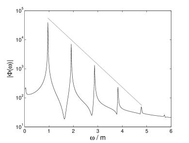
Figure 13: The power spectrum of the field at the center of the oscillon, $r=0$, in $\phi^{4}$ theory in three dimensions. The grey straight line is a guide to eye of the exponential $\exp(-b\,\omega)$ with the slope $b=1.8$.

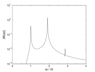
Figure 14: The power spectrum of the field far away from the oscillon core at $r=80$, in $\phi^{4}$ theory in three dimensions.

The oscillation frequency as a function of time is shown in Figure 12. The frequency approaches $\omega\simeq 0.97$ towards the end of the simulation before the oscillon decays. The fluctuations in the amplitude are naturally imprinted into the frequency. However, these do not prevent reaching a reasonable power law fit to the data over the whole span of the oscillon life time. In the best-fit the asymptotic value of the frequency is $\omega^{\star}=1.030\pm 0.003$ and the exponent governing the power law $\gamma=0.20\pm 0.01$. The power law is demonstrated in the inset in Figure 12. Like in the case of the amplitude, the asymptotic value of the frequency $\omega^{\star}$ remains physically meaningless as $\omega^{\star}>1$; the oscillon has a finite lifetime and decays even before the frequency reaches the threshold for radiation $\omega=1$. For more extensive studies of oscillons in quartic theory in three dimensions, in particular the effect of the initial radius and amplitude, see Gleiser and Sicilia (2009).

While the decay of the oscillon in three dimensions restricts the length of the time interval we can observe the evolution, this fate merely enhances the importance to examine the frequency spectrum of the oscillon before its demise. Due to the relatively fast energy loss the oscillation frequency shifts steadily and to overcome this effect we perform the Fourier transform over the interval of length $200$ in time units (the choice of the shorter interval naturally compromises the resolution we can expect on the frequency axis compared with the analysis in two dimensions). We choose to start the interval at time $t=4000$, thus this interval is in the middle of the phase of relative subdued radiation appearing as the plateau in energy in Figure 9.

The power spectrum at the center of the oscillon, $r=0$, is shown in Figure 13. It is qualitatively similar to the spectrum in two dimensions (Figure 6) with peaks located at multiples of the oscillation frequency, which is here located approximately at $\omega_{0}\simeq 0.955$. There are even similar patterns between the peaks as those seen in two dimensions. In addition, the suppression of the amplitudes which the peaks appear is still exponential as well, the best fit value of the slope being $-1.8$, very comparable with the value obtained in the two-dimensional theory. Unsurprisingly, the form of the power spectrum is dictated by the potential rather than the dimensionality of the theory.

The major difference between two and three dimensions is the far larger emitted radiation taking place in the latter resulting to a greatly larger width of the peaks in frequency space. This has been considered analytically in Gleiser and Sicilia (2008, 2009) in the case of the oscillation frequency.

Figure 14 shows the Fourier transform of the field $\phi$ obtained in the same time interval as in Figure 13, but at the location $r=80$. The strength of radiation shows simply in the far larger absolute values of the amplitudes compared with the situation in two dimensions, see Figure 8. There are three distinctive peaks present in the spectrum. There is a substantial structure rising immediately above the threshold for radiation at $\omega=1$. The origin of it can be traced to the large width of the peak of the basic oscillation frequency in Figure 13, the part of this peak for which $\omega>1$ overflows in the form of free radiation (for a quantitative study, see Gleiser and Sicilia (2009)). The radiation signal at $\omega\simeq 1$ is far stronger than in two dimensions. However, also in three dimensions the dominant peak is at the frequency corresponding the double of the oscillation frequency, $2\omega_{0}$. The height of this peak is several factors larger than the one at $\omega=1$. Moreover, as waves moving at frequency $\omega=2\omega_{0}$ carry far larger amount of energy than those barely in the free, propagating domain at $\omega\gtrsim 1$, we conclude that the dominant channel for the energy loss in three dimensions is also through the frequency band at $\omega\simeq 2\omega_{0}$. Finally, there is inferior, but still a visible peak in the spectra at $\omega=3\omega_{0}$.

IV sine-Gordon model

Sine-Gordon model is of considerable interest from the point of view of oscillating solutions both on theoretical and phenomenological grounds: in one-dimension it has a stable breather solution and it is also the potential of axion field (formation of oscillating energy concentrations in axion field were studied in Kolb and Tkachev (1994)). In Piette and Zakrzewski (1998) a fine-tuned initial ansatz was reported to create almost dissipationless breather in two dimensions. Here we start with the same Gaussian ansatz as in $\phi^{4}$ theory given by (5) with $r_{0}\simeq 2.9$ and $C=1$. We scale the potential of sine-Gordon model

$$V(\phi)=\frac{\Lambda^{4}}{\alpha^{2}}\big{(}1-\cos(\alpha\phi)\big{)}$$ (7)

to

$$V(\phi)=\frac{1}{\pi^{2}}\big{(}1+\cos(\pi\phi)\big{)}\,,$$ (8)

so that locations of the minima are the same as in $\phi^{4}$ theory, but here the mass $m^{2}=1$.

IV.1 Properties in two dimensions

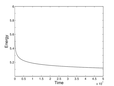
Figure 15: The energy inside a shell of radius $r=5r_{0}$ in sine-Gordon model in two dimensions over the span of the simulation up to $5\cdot 10^{7}$ time units.

Figure 16: The difference of the energy inside a shell of radius $r=5r_{0}$ and the constant $E_{0}=4.769$ in sine-Gordon model in two dimensions. The grey straight line is a guide to eye of a power law $(E-E_{0})\sim t^{-\delta}$ with the slope $\delta=0.119$.

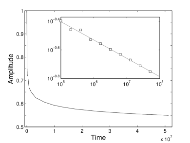
Figure 17: The amplitude as a function of time in sine-Gordon model in two dimensions. The inset shows the data points in the fit $A-A_{0}$ for $A_{0}=0.37$ for time greater than $10^{5}$. The grey straight line is the best fit power law $(A-A_{0})\sim t^{-\varrho}$ with the slope $\varrho=0.13$.

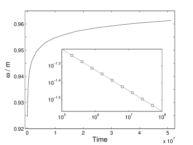
Figure 18: The oscillation frequency as a function of time in sine-Gordon model in two dimensions. The inset shows the data points in the fit $\omega^{\star}-\omega$ for $\omega^{\star}=0.991$ for time greater than $10^{5}$. The grey straight line is the best fit power law $(\omega^{\star}-\omega_{0})\sim t^{-\gamma}$ with the slope $\gamma=0.122$.

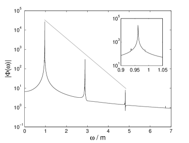
Figure 19: The power spectrum of the field at the center of the oscillon, $r=0$, in sine-Gordon model in two dimensions. The grey straight line is a guide to eye of the exponential $\exp(-b\,\omega)$ with the slope $b=2.1$. The inset shows the spectrum around the oscillation frequency $\omega_{0}\simeq 0.96$.

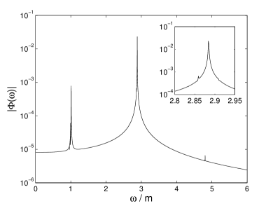
Figure 20: The power spectrum of the field far away from the oscillon core at $r=80$, in sine-Gordon model in two dimensions. The inset shows the spectrum around the location of the most prominent peak at $\omega\simeq 2.88$.

Figure 15 shows the energy inside the shell with radius $r=5r_{0}$ in the simulation up to $5\cdot 10^{7}$ time units. This is qualitatively very similar to the case in quartic theory. We sought again for a power law using least-square fit. The result is presented in Figure 16 where the constant $E_{0}=4.769$ is subtracted from the energy inside the shell. The resulting curve has the slope $-0.119$ on the logarithmic scale, demonstrated by the grey straight line in the figure. We lack some of the dynamical range reached in the simulation in $\phi^{4}$ theory, but there is evidence for a power law roughly over three orders of magnitude in time with an exponent $\delta=0.119\pm 0.003$. The rate of decrease is marginally smaller than what we observed in $\phi^{4}$ theory, and the asymptotic energy of the oscillon, $E_{0}=4.77\pm 0.01$, is now slightly larger, but generally oscillons in both models are comparatively similar lumps of energy.

The amplitude of the oscillations behaves also very similar way compared with the quartic theory in two dimensions. Figure 17 shows the amplitude over the course of time. The inset demonstrates the best-fit power law where $A_{0}=0.37\pm 0.10$ and $\varrho=0.13\pm 0.05$. The derived errors in the fit are quite large, it can be seen that there is substantial scatter around the central value for time $<10^{6}$, the oscillon in sine-Gordon model has a larger asymptotic amplitude $A_{0}$ than in $\phi^{4}$ theory.

The evolution of the frequency as a function of time is shown in Figure 18. Like in the case of energy, the rate of change is less than in quartic theory and the oscillation frequency reaches value $\omega=0.961$ at the end of the simulation at time point $t=5.12\cdot 10^{7}$. The search for a critical frequency and an associated power law here yields quite a stringent results. There is a remarkably good fit to the data with $\omega^{\star}=0.991\pm 0.002$ and $\gamma=0.120\pm 0.004$. The data points for $\omega^{\star}-\omega(t)$ are shown in the inset of Figure 18 together with the grey straight line that demonstrates the power law $t^{-\gamma}$. This suggests now that there exists a critical frequency $\omega^{\star}<1$ in two-dimensional sine-Gordon model that would correspond an oscillon with a minimum energy.

The power spectrum of the oscillon in sine-Gordon model is shown in Figure 19 obtained by a Fourier transform in an interval of length $5000$ in time units starting at time $t=5.12\cdot 10^{7}$. There are no even multiples of the oscillation frequency $\omega_{0}$ present in the spectra. This is simply due to the symmetry of the potential (7) in sine-Gordon model with respect to its minima - there cannot be non-zero terms $f_{n}(r)$ in (6) for an even $n$. The remaining peaks are exponentially suppressed as a function of frequency $\omega$. This suppression is even quantitatively very similar to the one in quartic theory. The small difference in the slope we measure is well within the limits of uncertainty we can expect in evaluating the height of the narrow peaks.

Figure 20 shows the Fourier transform of the field in the same time interval as Figure 19, but at location $r=80$. Now the most dominant peak is at $\omega=2.88=3\omega_{0}$, the first radiative mode as the even multiples of $\omega_{0}$, including $2\omega_{0}$, do not exist. There is still a visible pinnacle at $5\,\omega_{0}$ and a substantial peak just above the radiation frequency $\omega=1$, but exactly like in $\phi^{4}$ theory that one is more than order of magnitude suppressed compared with the prominent one at the frequency $3\omega_{0}$. Also in sine-Gordon model it is the first non-zero multiple of the basic frequency $\omega_{0}$ above the threshold for radiation that leaks the energy from the oscillon.

The Gaussian ansatz (5) does not create long-lived oscillons in sine-Gordon model in three dimensions. For an investigation with fine-tuned initial conditions see Piette and Zakrzewski (1998).

V A Convex Potential

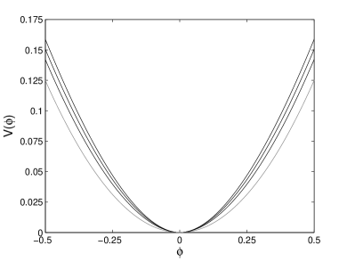
Figure 21: Potential $V(\phi)$ in (10) around the minimum for values $p=0.4,0.3,0.2$ (from top to bottom). They grey line shows the quadratic potential $\phi^{2}/2$.

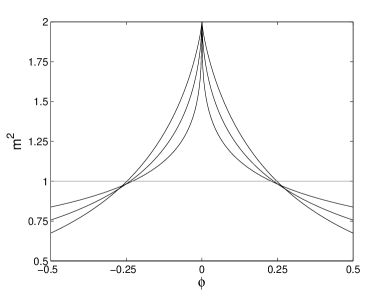
Figure 22: The second derivative of the potential $V(\phi)$ in (10) for $p=0.4,0.3,0.2$ (from broader to narrower spikes). The grey line shows the constant $m^{2}=1$ for a quadratic potential.

Majority of the studies on oscillons has been carried out in the context of $\phi^{4}$ theory (see e.g. Gleiser (1994); Copeland et al. (1995); Fodor et al. (2006); Saffin and Tranberg (2007)) or in sine-Gordon model. Both potentials (3) and (7) have degenerate vacua and inflections points. In Kasuya et al. (2003) the study dealt potentials that are nearly quadratic. In particular a quadratic potential with a negative logarithmic correction was reported to support long-lived lumps (called I-balls by the authors). Very recently there has been interest in convex potentials and a study Amin et al. (2011a) considered the formation of oscillons in the following potential

$$V(\phi)=\frac{m^{2}M^{2}}{2\beta}\left[\left(1+\frac{\phi^{2}}{M^{2}}\right)^{\beta}-1\right]\,,$$ (9)

which is motivated by a number of supergravity and superstring scenarios.

It was the work in Kasuya et al. (2003) that initially lead us to study the effects of the form of potential on the existence of long-lived oscillating solutions. We have chosen to study the following convex function

$$V(\phi)=\frac{\phi^{2}}{1+\phi^{2p}}\,,$$ (10)

which reduces to quadratic when exponent $p=0$. Figure 21 shows the potential (10) close to its minimum for values $p=0.4,0.3$ and $0.2$ together with the quadratic potential $\phi^{2}/2$ indicated by the grey line. The potential is steeper than quadratic one in the vicinity of the minimum where oscillations of the field take place, $|\phi|<1$.

The potential (10) sets far greater challenge for the absorbing boundary conditions than $\phi^{4}$ theory or sine-Gordon model. This becomes readily apparent in Figure 22 where the second derivative of the potential is shown for the same values of parameter $p$. Already small deviations from the vacuum $\phi=0$ create large variations in $V^{\prime\prime}$, the greater the smaller parameter $p$ is. This is a drawback from the point of view of the absorbing boundary conditions used because they are based on the assumption that the potential can be linearised in the equation of motion. Once the fluctuations create large corrections, the absorption can be expected to be only partial or, in the worst case, the update on the boundary even pumps energy into the lattice. We restrict considerations from now on to values $1/2>p\geq 0.4$ which yield less stark variations and for which the radiation is clearly adequately removed from the lattice. Potential (10) is also more time consuming to evaluate numerically and consequently the simulations do not reach such a long final time as the one presented in $\phi^{4}$ theory, but typically order of $10^{6}$ time units.

V.1 Properties in two dimensions

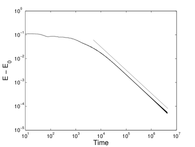
Figure 23: The difference of the energy inside a shell of radius $r=5r_{0}$ and the constant $E_{0}=3.80343$ in the convex potential (10) for $p=0.45$ in two dimensions. The grey straight line is a guide to eye of a power law $(E-E_{0})\sim t^{-\delta}$ with the slope $\delta=0.97$.

Also here the oscillon is initialised by a Gaussian deviation from the vacuum

$$\phi(r)=C\cdot\exp(-r^{2}/r_{0}^{2}),$$ (11)

with the same width as before $r_{0}\simeq 2.9$, but due to the steepness of the potential (10) we set the amplitude of the displacement to be smaller, $C=0.6$. The oscillons formed are well described by a Gaussian shape though with a slightly larger width and a longer tail. After a short initial phase of radiation the oscillon settles into a state characterised by a very constant energy. We present the data from simulation when the exponent was set to $p=0.45$. The energy inside the radius $r=5r_{0}$ for this choice remains above $E=3.8$. We carried out the least-square fit for the energy. Now far more fine-tuning is required for seeking the asymptotic energy $E_{0}$. Figure 23 shows the constant $E_{0}=3.80343$ subtracted from the energy inside the shell. The radiative component decays now almost inversely proportional to time, the best fit exponent being $\delta=0.97$ and the corresponding power law demonstrated by the grey line in the figure. There is agreement with this power law over two orders of magnitude in time during which the difference $\left(E(t)-E_{0}\right)$ drops below $10^{-4}$. The best-fit values for the asymptotic energy and the exponent governing the power law are $E_{0}=3.80343(4)$ and $\delta=0.974\pm 0.003$, respectively. The diminutive uncertainty in the value of energy reflects the fine-tuning needed in the fit, and in turn the stability of the value the energy reaches in the simulation.

Nearly constant energy implies also very stable oscillation frequency. After initial phase the oscillation frequency settles to $\omega_{0}=0.879$ and we do not observe any increase in this, but within the accuracy to determine frequencies it remains the same until the end of the simulation beyond time $t=4\cdot 10^{6}$. It is noteworthy that this value is considerably below the threshold for radiation. The amplitude of the oscillations settles to a value $A\simeq 0.49$.

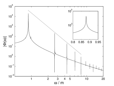
Figure 24: The power spectrum of the field at the center of the oscillon, $r=0$, in the convex potential (10) for $p=0.45$ in two dimensions. The grey straight line is a guide to eye of the power law $\omega^{-\kappa}$ with the slope $\kappa=4.6$. The inset shows the spectrum around the oscillation frequency $\omega_{0}\simeq 0.88$.

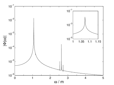
Figure 25: The power spectrum of the field far away from the oscillon core at $r=80$, in the convex potential (10) for $p=0.45$ in two dimensions. The inset shows the spectrum around the most prominent peak at frequency $\omega\simeq 1.07$.

We show the power spectrum of the oscillon in the potential (10) for $p=0.45$ obtained in the previously used time interval starting at time $t=4\cdot 10^{6}$ in Figure 24. Because the potential (10) is symmetric around its minimum, there are only peaks at odd multiples of the oscillation frequency as in sine-Gordon model. But it is surprising that the suppression is governed by a power law, we plot also the frequency axis on a logarithmic scale in Figure 24. On the basis of the stability and weak radiation from the oscillon a strong exponential suppression of radiative modes would have been likely. The power law decrease as a function of the frequency is considerably quick though, the amplitudes are suppressed roughly as $\omega^{-5}$ though the exponent should be considered only indicative.

Figure 25 shows the frequencies present far away from the oscillon core at $r=80$. There is a peak at frequency $\omega=2.64$, thus at $3\omega_{0}$, but this one is not the dominant. Instead the amplitude of the peak just above the radiation frequency at $\omega=1.07$ is over seventy times higher. The dominant radiative mode is not related to multiples of the oscillation frequency $\omega_{0}$.

V.2 Properties in three dimensions

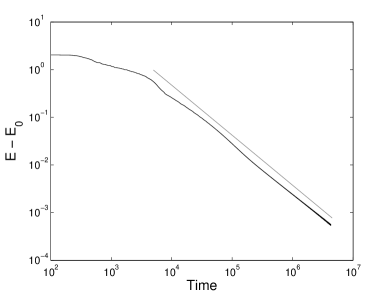
Figure 26: The difference of the total energy and the constant $E_{0}=13.908$ in the convex potential (10) for $p=0.45$ in three dimensions. The grey straight line is a guide to eye of a power law $(E-E_{0})\sim t^{-\delta}$ with the slope $\delta=1.05$.

We use the same Gaussian initial ansatz (11) with the same width and amplitude as in two dimensions. This initial profile creates now an oscillating lump also in three dimensions though the oscillon has a larger width and a longer tail than the Gaussian distribution. The data shown is for the same value $p=0.45$ in the potential (10). After initial stronger radiative phase, there remains energy above the value $E=13.9$ within the radius $r=5r_{0}$.

For the least-square fit we use now the data on the total energy in the lattice because the oscillon is more spatially spread and due to the precision required in determining the value of the constant $E_{0}$ below $10^{-3}$ the fluctuations in the energy inside the shell become apparent (they are to a lesser extent already visible in Figure 23). Figure 26 shows the constant $E_{0}=13.908$ subtracted from the total energy. The decaying component decreases fast in time, the best-fit for the exponent governing the power law is $\delta=1.09\pm 0.01$ while the asymptotic value of the energy is $E_{0}=13.9081\pm 0.0002$. There is fairly large uncertainty in the value of the exponent, but there is good evidence that the radiative part decays faster than inversely proportional to time. The amplitude related to this energy is $A\simeq 0.34$.

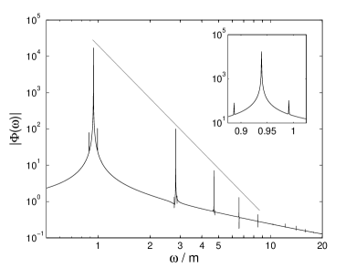
Figure 27: The power spectrum of the field at the center of the oscillon, $r=0$, in the potential (10) for $p=0.45$ in three dimensions. The grey straight line is a guide to eye of the power law $\omega^{-\kappa}$ with the slope $\kappa=4.85$. The inset shows the spectrum around the oscillation frequency $\omega_{0}\simeq 0.94$.

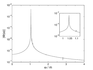
Figure 28: The power spectrum of the field far away from the oscillon core at $r=80$, in the potential (10) for $p=0.45$ in three dimensions. The inset shows the spectrum around the most prominent peak at frequency $\omega\simeq 1.04$.

With the aforementioned energy the oscillation frequency settles to $\omega\simeq 0.939$. Again we do not observe increase in the frequency within the numerical accuracy after the initial phase. Figure 27 shows the power spectrum of the three-dimensional oscillon obtained in the previously used time interval starting at time $t=4\cdot 10^{6}$. The result is very similar to Figure 24 with peaks at odd multiples of the basic frequency $\omega_{0}$. The suppression of the higher amplitudes is again governed by a power law demonstrated by the grey straight line in the figure. The measured slope is slightly steeper than in two dimensions, but this difference is hardly significant taking into account the accuracy of the data we can expect.

Figure 28 shows the frequencies at the location $r=80$. There is only barely visible structure above the background at $\omega\approx 2.82$, three times the value of the oscillation frequency. The only peak of any note is located at frequency $\omega=1.04$, thus barely above the threshold for propagating radiation.

To summarize our findings of the oscillons in the convex potential (10), the change from two to three dimensions seem to have surprisingly small effect. In both dimensions there remains a very stable lump of energy oscillating at a constant frequency which emits only tiny amount of radiation. While we do not have an explanation for their longevity, the investigation in frequency space gives one answer. As the oscillon can primarily only excite modes that are just above the threshold for radiation, i.e. $\left(\omega-m\right)\ll 1$, obviously such modes can carry only lesser amount of energy away from the core of the lump. Consequently we can expect far reduced emitted radiation compared with $\phi^{4}$ theory and sine-Gordon model as we indeed observe (it cannot be excluded that some of the signal we see is from relic radiation on the lattice that was not absorbed by the boundary, but reflected back to the grid).

We have considered here only very limited range of values of the parameter $p$ in the potential (10), but the potential supports oscillons in a wider variety of the values of the exponent $p$ governing its steepness Bennett . With a different choice for lattice spacing and time step, oscillons have survived up to $10^{7}$ time units Bennett . This is hardly a surprising result taking into account their minuscule radiation losses.

Finally, it should be noted that non-radiating oscillons has been found in one-dimensional signum-Gordon model Arodz et al. (2008) (more recently also a new class of swaying oscillons have been discovered in the same model Arodz and Swierczynski (2011)). It is defined by the potential

$$V(\phi)=g\,|\phi|.$$ (12)

The convex potential (10) reduces to linear for $p=1/2$ in the limit of large field, $|\phi|\gg 1$. This is not the realm where oscillations of the field take place, but it cannot be excluded right away that there were no connection between oscillons we have reported here and those described in Arodz et al. (2008). At very least, both are examples of oscillons appearing in theories where the potential is not a smooth one.

VI Conclusions

model	dim	$E_{0}$	$\delta$
quartic theory	$2$	$4.613\pm 0.003$	$0.1520\pm 0.0005$
quartic theory	$3$	$41.56\pm 0.05$	$0.65\pm 0.01$
sine-Gordon	$2$	$4.77\pm 0.01$	$0.119\pm 0.003$
convex potential	$2$	$3.803430\pm 4\cdot 10^{-6}$	$0.974\pm 0.003$
convex potential	$3$	$13.9081\pm 0.0002$	$1.09\pm 0.01$

Table 2: The values of the asymptotic energy $E_{0}$ and the exponent $\delta$ in $\left(E(t)-E_{0}\right)\sim t^{-\delta}$ for the oscillons in the various models studied with the initial conditions as mentioned in the text.

We have studied oscillons in $\phi^{4}$ theory, sine-Gordon model and in convex potentials, performing (1+1)-dimensional simulations assuming radial symmetry. An important ingredient was the development of absorbing boundary conditions for a massive, real scalar field. Generally absorbing boundary conditions work well and radiation is removed from the lattice.

We showed that the time evolution of the energy and the frequency of oscillons is well modelled by dividing it to a constant and a decaying radiative part. There is strong evidence that the decay of the radiative part is governed by a power law in all models considered. We further determined the values of the constant components as well as values of the exponents in the power law decay, which we summarize in Table 2. The power law decay has been previously reported in $\phi^{4}$ theory Gleiser and Sicilia (2008, 2009) and for flat-top oscillons in Amin and Shirokoff (2010). Note that for the oscillons in the convex potentials the frequency remains constant, which is a qualitatively new behaviour for an oscillon.

model	dimension	$A_{0}$	$\varrho$
quartic theory	2	$0.33\pm 0.06$	$0.13\pm 0.02$
quartic theory	3	$-1.4\pm 0.3$	$0.066\pm 0.007$
sine-Gordon	2	$0.37\pm 0.10$	$0.13\pm 0.05$

Table 3: The values of the asymptotic amplitude $A_{0}$ and the exponent $\varrho$ in $\left(A(t)-A_{0}\right)\sim t^{-\varrho}$ for the oscillons in the various models studied with the initial conditions as mentioned in the text.

model	$\omega^{\star}$	$\gamma$
quartic theory	$0.981\pm 0.003$	$0.18\pm 0.02$
sine-Gordon model	$0.991\pm 0.002$	$0.120\pm 0.004$

Table 4: The values of the critical frequency $\omega^{\star}$ and the exponent $\gamma$ in $\left(\omega^{\star}-\omega(t)\right)\sim t^{-\gamma}$ in two dimensions for the oscillons with the initial conditions as mentioned in the text.

We also studied the evolution of the amplitude and the oscillation frequency over time, our results are summarized in Tables 3 and 4. The oscillon amplitude also exhibits a power law decay, which in three dimensions is strongly modulated by a beat frequency, while in the case of the convex potential it is constant.

Furthermore, we examined the power spectrum of field at the centre of oscillon and near the boundary. While in $\phi^{4}$ theory and in sine-Gordon model there is an exponential attenuation of higher multiples of the oscillation frequency, the oscillons in the convex potential show only a power law suppression.

Understanding the manner oscillons radiate and shed their energy away is crucial in gaining insight for their persistence and longevity. We studied the outgoing radiation in frequency space. The emitted radiation in $\phi^{4}$ theory and in sine-Gordon model is strongly peaked at the first non-zero multiple of the basic frequency, while in the convex potential the oscillons radiate at a low frequency just above the threshold to release radiation. Our results in quartic theory, in particular in two dimensions, agree well with the study of quasi breathers in the same model Saffin and Tranberg (2007). There it was identified that the emissions take place at the frequencies $n\omega_{0}$, with $n\geq 2$ with the frequency $2\omega_{0}$ being the dominant one. The quasi breather approach, i.e. ansatz (6), does not assign any width for the frequencies. This was considered the starting point in the work Gleiser and Sicilia (2009) when dealing with the basic oscillation frequency. Our results indicate that there is a contribution from both sources, from higher modes as well as from the spread related to the basic oscillation frequency and once again highlight the richness and complexity of oscillons. An approach that would account for both higher frequencies present in the spectra as well as the width of the frequencies might capture the problem of oscillon radiation in full.

What do the results tell about the lifetime of oscillons? The appearance of the constant $E_{0}$ now raises the question of its physical interpretation. While it would be tempting to define it as the energy of a non-radiating oscillon, this kind of conclusion cannot be made straightforwardly. It is namely not obvious at all that there are oscillon solutions at such energy. While the energy decreases the oscillon oscillates faster and the oscillation frequency $\omega_{0}$ increases. Once close enough to the threshold for radiation $\omega=m$ oscillon demises when it reaches its minimum energy state Watkins (1996); Saffin and Tranberg (2007). This was well demonstrated in $\phi^{4}$ theory in three dimensions, there the asymptotic energy $E_{0}$ is well below the energy level that caused the oscillon to dissolve. Because the radiative part shows a slow decay in time in two dimensions, the energy oscillons have reached at the end of simulations is still well above the asymptotic value $E_{0}$ in $\phi^{4}$ theory and sine-Gordon model, more precisely by $13\%$ and $7\%$, respectively (it should be noted that there are some theoretical bounds on the minimum energy of lumps Buniy and Kephart (2003)).

However, the case for the convex potentials presented here is definitely intriguing. We have shown that there the suppression of the radiation losses is quick, roughly inversely proportional to time. Thus only very small further decrease in energy is to be expected to occur, orders of magnitude less than in $\phi^{4}$ theory or in sine-Gordon model. Furthermore, the frequency of oscillons is well below the threshold for radiation. This all makes it possible that these oscillons could go on indefinitely long. Another open question remaining is if it is possible to tailor potentials in which the emission of radiation from oscillon is strongly suppressed also in higher dimensions. The convex potential we considered is not phenomenologically particularly well motivated, but if this sort of oscillons can also appear in more realistic theories their long life-time would almost certainly make them viable to affect physics in the system there.

Appendix A Absorbing Boundaries

In this appendix the absorbing boundary conditions are presented. As the starting point consider the following linear wave equation

$$\ddot{\varphi}-\nabla^{2}\varphi+\varphi\cdot V^{\prime\prime}|_{\varphi=0}=0\,,$$ (13)

where $\varphi$ is now a small perturbation around a chosen vacuum and $V^{\prime\prime}$ evaluated at that point. For example in $\phi^{4}$ theory $\phi\rightarrow v-\varphi$ and $V^{\prime\prime}(\phi)|_{\phi=v}=2\lambda v^{2}=m^{2}$. The treatment here follows closely the one presented in Battye (1995) for a massless scalar field (for absorbing boundary conditions in general see also Bamberger et al. (1990)).

A.1 Cylindrical Wave

When one assumes radial symmetry in two space dimensions the wave equation (13) reads

$$\frac{{\partial^{2}\varphi}}{{\partial t^{2}}}-\frac{{\partial^{2}\varphi}}{{\partial r^{2}}}-\frac{1}{r}\frac{{\partial\varphi}}{{\partial r}}+m^{2}\varphi=0.$$ (14)

The solutions of (14) are Bessel functions, but considering an absorbing boundary at far distance ($r\gg 1$) the approximative solution reads

$$\varphi(t,r)=\frac{1}{\sqrt{r}}\exp\Big{[}\,i\,(\sqrt{\omega^{2}-m^{2}}\,r+\omega t\,)\Big{]}\,,$$ (15)

where $\omega$ is a dual variable to $t$. This solution (15) is annihilated at the boundary $r=r_{\rm b}$ (to order $r^{-5/2}$) by the operator in the parenthesis

$$\Bigg{[}\frac{{\partial}}{{\partial r}}-i\sqrt{\omega^{2}-m^{2}}+\frac{1}{2r}\,\Bigg{]}\varphi_{\Big{|}_{r=r_{\rm b}}}=0.$$ (16)

From the point of view of numerical implementation using leap frog update we aim to second order equations at the boundary. Expanding the square root to second order in (16) and replacing the variable $\omega$ by the corresponding time derivative one obtains an absorbing boundary condition on the edge of the one-dimensional grid

$$\frac{{\partial}}{{\partial t}}\frac{{\partial\varphi}}{{\partial r}}+\frac{{\partial^{2}\varphi}}{{\partial t^{2}}}-\frac{1}{2}m^{2}\varphi+\frac{1}{2r}\frac{{\partial\varphi}}{{\partial t}}=0.$$ (17)

The equation (17) permits a straightforward time evolution using leap frog algorithm. To be more precise, the condition (17) yields a new evolution equation for the field momentum $\Pi$ compared to that in the interior of the lattice, whereas the update of the field $\phi$ stays unaltered. The last term in (17), suppressed by inverse of physical distance $r$, results from the treatment in the polar coordinates. It turns out to be fairly insignificant with the numerical set-up used in this study, but in a smaller grids it increases the absorption.

A.2 Spherical Wave in Three Dimensions

When one assumes spherical symmetry in three dimensions the solution for the wave equation

$$\frac{{\partial^{2}\varphi}}{{\partial t^{2}}}-\frac{{\partial^{2}\varphi}}{{\partial r^{2}}}-\frac{2}{r}\frac{{\partial\varphi}}{{\partial r}}+m^{2}\varphi=0.$$ (18)

is given by

$$\varphi\left(t,r\right)=\frac{1}{r}\exp\Big{[}\,i\,(\sqrt{\omega^{2}-m^{2}}\,r+\omega t\,)\Big{]}\,.$$ (19)

This is annihilated at the boundary $r=r_{\rm b}$ by

$$\Bigg{[}\frac{{\partial}}{{\partial r}}-i\sqrt{\omega^{2}-m^{2}}+\frac{1}{r}\,\Bigg{]}\varphi_{\Big{|}_{r=r_{\rm b}}}=0\,,$$ (20)

which leads to following absorbing boundary condition

$$\frac{{\partial}}{{\partial t}}\frac{{\partial\varphi}}{{\partial r}}+\frac{{\partial^{2}\varphi}}{{\partial t^{2}}}-\frac{1}{2}m^{2}\varphi+\frac{1}{r}\,\frac{{\partial\varphi}}{{\partial t}}=0,$$ (21)

appropriate when a three-dimensional system is considered in a spherically symmetric geometry.

References

- Derrick (1964) G. H. Derrick, J. Math. Phys. 5, 1252 (1964).
- Coleman (1985) S. R. Coleman, Nucl. Phys. B262, 263 (1985).
- Multamaki and Vilja (2000) T. Multamaki and I. Vilja, Nucl. Phys. B574, 130 (2000), eprint hep-ph/9908446.
- Tsumagari et al. (2008) M. I. Tsumagari, E. J. Copeland, and P. M. Saffin, Phys. Rev. D78, 065021 (2008), eprint 0805.3233.
- Dine and Kusenko (2004) M. Dine and A. Kusenko, Rev. Mod. Phys. 76, 1 (2004), eprint hep-ph/0303065.
- Gleiser (1994) M. Gleiser, Phys. Rev. D49, 2978 (1994), eprint hep-ph/9308279.
- Segur and Kruskal (1987) H. Segur and M. D. Kruskal, Phys. Rev. Lett. 58, 747 (1987).
- Bogolyubsky and Makhankov (1976) I. L. Bogolyubsky and V. G. Makhankov, JETP Lett. 24, 12 (1976).
- Bogolyubsky and Makhankov (1977) I. L. Bogolyubsky and V. G. Makhankov, Pisma Zh. Eksp. Teor. Fiz. 25, 120 (1977).
- Fodor et al. (2006) G. Fodor, P. Forgacs, P. Grandclement, and I. Racz, Phys. Rev. D74, 124003 (2006), eprint hep-th/0609023.
- Fodor et al. (2008) G. Fodor, P. Forgacs, Z. Horvath, and A. Lukacs, Phys. Rev. D78, 025003 (2008), eprint 0802.3525.
- Fodor et al. (2009a) G. Fodor, P. Forgacs, Z. Horvath, and M. Mezei, Phys. Rev. D79, 065002 (2009a), eprint 0812.1919.
- Fodor et al. (2009b) G. Fodor, P. Forgacs, Z. Horvath, and M. Mezei, Phys. Lett. B674, 319 (2009b), eprint 0903.0953.
- Di Plinio et al. (2010) F. Di Plinio, G. S. Duane, and R. Temam (2010), eprint 1009.2529.
- Honda (2010) E. P. Honda, Phys. Rev. D82, 024038 (2010), eprint 1006.2421.
- Fodor et al. (2010) G. Fodor, P. Forgacs, and M. Mezei, Phys. Rev. D81, 064029 (2010), eprint 0912.5351.
- Grandclement et al. (2011) P. Grandclement, G. Fodor, and P. Forgacs (2011), eprint 1107.2791.
- Valdez-Alvarado et al. (2011) S. Valdez-Alvarado, R. Becerril, and L. A. Urena-Lopez (2011), eprint 1107.3135.
- Fodor et al. (2009c) G. Fodor, P. Forgacs, Z. Horvath, and M. Mezei, JHEP 08, 106 (2009c), eprint 0906.4160.
- Amin and Shirokoff (2010) M. A. Amin and D. Shirokoff, Phys. Rev. D81, 085045 (2010), eprint 1002.3380.
- Hertzberg (2010) M. P. Hertzberg, Phys. Rev. D82, 045022 (2010), eprint 1003.3459.
- Enqvist and Mazumdar (2003) K. Enqvist and A. Mazumdar, Phys. Rept. 380, 99 (2003), eprint hep-ph/0209244.
- Farhi et al. (2005) E. Farhi, N. Graham, V. Khemani, R. Markov, and R. Rosales, Phys. Rev. D72, 101701 (2005), eprint hep-th/0505273.
- Graham (2007a) N. Graham, Phys. Rev. Lett. 98, 101801 (2007a), eprint hep-th/0610267.
- Graham (2007b) N. Graham, Phys. Rev. D76, 085017 (2007b), eprint arXiv:0706.4125 [hep-th].
- Gleiser and Thorarinson (2007) M. Gleiser and J. Thorarinson, Phys. Rev. D76, 041701 (2007), eprint hep-th/0701294.
- Gleiser and Thorarinson (2009) M. Gleiser and J. Thorarinson, Phys. Rev. D79, 025016 (2009), eprint 0808.0514.
- Gleiser et al. (2011) M. Gleiser, N. Graham, and N. Stamatopoulos, Phys. Rev. D83, 096010 (2011), eprint 1103.1911.
- Broadhead and McDonald (2005) M. Broadhead and J. McDonald, Phys. Rev. D72, 043519 (2005), eprint hep-ph/0503081.
- Amin et al. (2010) M. A. Amin, R. Easther, and H. Finkel, JCAP 1012, 001 (2010), eprint 1009.2505.
- Amin et al. (2011a) M. A. Amin, R. Easther, H. Finkel, R. Flauger, and M. P. Hertzberg (2011a), eprint 1106.3335.
- Graham and Stamatopoulos (2006) N. Graham and N. Stamatopoulos, Phys. Lett. B639, 541 (2006), eprint hep-th/0604134.
- Farhi et al. (2008) E. Farhi et al., Phys. Rev. D77, 085019 (2008), eprint 0712.3034.
- Saffin et al. (2008) P. M. Saffin, A. Padilla, and E. J. Copeland, JHEP 09, 055 (2008), eprint 0804.3801.
- Gleiser and Howell (2005) M. Gleiser and R. C. Howell, Phys. Rev. Lett. 94, 151601 (2005), eprint hep-ph/0409179.
- Dymnikova et al. (2000) I. Dymnikova, L. Koziel, M. Khlopov, and S. Rubin, Grav. Cosmol. 6, 311 (2000), eprint hep-th/0010120.
- Amin et al. (2011b) M. A. Amin, P. Zukin, and E. Bertschinger (2011b), eprint 1108.1793.
- Dutta et al. (2008) S. Dutta, D. A. Steer, and T. Vachaspati, Phys. Rev. Lett. 101, 121601 (2008), eprint 0803.0670.
- Carvalho and Perivolaropoulos (2009) C. S. Carvalho and L. Perivolaropoulos, Phys. Rev. D79, 065032 (2009), eprint 0901.4109.
- Romanczukiewicz and Shnir (2010) T. Romanczukiewicz and Y. Shnir, Phys. Rev. Lett. 105, 081601 (2010), eprint 1002.4484.
- Hindmarsh and Salmi (2006) M. Hindmarsh and P. Salmi, Phys. Rev. D74, 105005 (2006), eprint hep-th/0606016.
- Watkins (1996) R. Watkins, DART-HEP-96/03, unpublished (1996).
- Saffin and Tranberg (2007) P. M. Saffin and A. Tranberg, JHEP 01, 030 (2007), eprint hep-th/0610191.
- Gleiser and Sicilia (2008) M. Gleiser and D. Sicilia, Phys. Rev. Lett. 101, 011602 (2008), eprint 0804.0791.
- Gleiser and Sicilia (2009) M. Gleiser and D. Sicilia, Phys. Rev. D80, 125037 (2009), eprint 0910.5922.
- Gleiser and Sornborger (2000) M. Gleiser and A. Sornborger, Phys. Rev. E62, 1368 (2000), eprint patt-sol/9909002.
- Copeland et al. (1995) E. J. Copeland, M. Gleiser, and H. R. Muller, Phys. Rev. D52, 1920 (1995), eprint hep-ph/9503217.
- Honda and Choptuik (2002) E. P. Honda and M. W. Choptuik, Phys. Rev. D65, 084037 (2002), eprint hep-ph/0110065.
- Hindmarsh and Salmi (2008) M. Hindmarsh and P. Salmi, Phys. Rev. D77, 105025 (2008), eprint 0712.0614.
- Aarts and Smit (1998) G. Aarts and J. Smit, Nucl. Phys. B511, 451 (1998), eprint hep-ph/9707342.
- Aarts (2001) G. Aarts, Phys. Lett. B518, 315 (2001), eprint hep-ph/0108125.
- Kolb and Tkachev (1994) E. W. Kolb and I. I. Tkachev, Phys. Rev. D49, 5040 (1994), eprint astro-ph/9311037.
- Piette and Zakrzewski (1998) B. Piette and W. J. Zakrzewski, Nonlinearity 11, 1103 (1998).
- Kasuya et al. (2003) S. Kasuya, M. Kawasaki, and F. Takahashi, Phys. Lett. B559, 99 (2003), eprint hep-ph/0209358.
- (55) R. Bennett, private communication.
- Arodz et al. (2008) H. Arodz, P. Klimas, and T. Tyranowski, Phys. Rev. D77, 047701 (2008), eprint 0710.2244.
- Arodz and Swierczynski (2011) H. Arodz and Z. Swierczynski (2011), eprint 1106.3169.
- Buniy and Kephart (2003) R. V. Buniy and T. W. Kephart, Phys. Rev. D68, 105015 (2003), eprint hep-th/0303195.
- Battye (1995) R. Battye, Ph.D. thesis, University of Cambridge (1995).
- Bamberger et al. (1990) A. Bamberger, P. Joly, and J. E. Roberts, SIAM Journal on Numerical Analysis 27, 323 (1990).