HIP-2012-02/TH

Perturbative Improvement of the Schrödinger Functional for Lattice Strong Dynamics

Abstract

Lattice simulations on SU(2) and SU(3) gauge theories with matter fields in the fundamental, adjoint and two index symmetric representations are needed to determine if these theories are near or within the conformal window as required for their applications in beyond standard model phenomenology. Simulations with Wilson fermion action are subject to artifacts linear in the lattice spacing $a$, and must be improved. We provide the necessary coefficients for perturbative improvement of the boundary terms when using Schrödinger functional boundary conditions and furthermore show that correctly implemented ${\mathcal{O}}(a)$ improved actions are necessary for reliable results.

There has recently been interest in studying quantum field theories with a nontrivial infrared fixed point (IRFP), both in continuum and on the lattice. Under the renormalization group evolution, the coupling of these theories shows asymptotic freedom at small distances, analogously to QCD, but flows to a fixed point at large distances where the theory hence looks conformal. Such theories have applications in beyond Standard Model model building. These include unparticles, i.e. an infrared conformal sector coupled weakly to the Standard Model Georgi:2007ek , and (extended) technicolor scenarios, that explain the masses of the Standard Model gauge bosons and fermions via strong coupling gauge theory dynamics TC ; Hill:2002ap ; Sannino:2008ha . In addition to direct applications to particle phenomenology, the phase diagrams of gauge theories, as a function of the number of colours, $N$, flavours $N_{f}$ and fermion representations, are interesting from the purely theoretical viewpoint of understanding the nonperturbative gauge theory dynamics from first principles.

Several methods to estimate the vacuum phase diagram of a gauge theory exist. A traditional method is the ladder approximation to the Schwinger-Dyson equation for the fermion propagator yielding an estimate for the onset of chiral symmetry breaking and signaling the departure from conformal to confining phase Appelquist:1998rb ; Sannino:2004qp . However, the only truly first principle method is constituted by lattice simulations. Several initial studies have appeared in literature: for example SU(2) with fundamental representation fermions Bursa:2010xr ; Karavirta:2011zg , SU(2) with adjoint fermions Catterall:2007yx ; Hietanen:2008mr ; DelDebbio:2008zf ; Catterall:2008qk ; Hietanen:2009az ; DeGrand:2011qd and SU(3) with fermions in the fundamental Appelquist:2007hu ; Fodor:2009wk ; Deuzeman:2008sc or in the two-index symmetric Shamir:2008pb , i.e. the sextet, representation.

The studies with Wilson fermions are subject to lattice artifacts proportional to the lattice spacing $a$. In the context of high precision results for QCD like theories, i.e. SU(N) gauge theory with modest number of flavors, a program to cancel these lattice artifacts has been devised Sheikholeslami:1985ij ; Luscher:1992an . The basic idea in this approach is to introduce local counterterms whose coefficients will be fine tuned to cancel all ${\cal O}(a)$ contributions. In this Letter we provide the values of the perturbative coefficients required in the analyses of SU(2) and SU(3) gauge theories with fermions in the fundamental, adjoint and two-index symmetric representations. In addition to these results, we highlight their significance: The improved actions neglecting some of the counterterms will not work and, moreover, the boundary conditions for the background field when using Schrödinger functional, must be chosen carefully. This point has been emphasised also in Sint:2011gv .

The basic Wilson lattice action is $S_{0}=S_{\textrm{G}}+S_{\textrm{F}}$, where $S_{\textrm{G}}$ denotes the standard Wilson plaquette action and $S_{\textrm{F}}$ is the usual Wilson fermion action for $N_{f}$ (mass degenerate) Dirac fermions in the fundamental or higher representation of the gauge group.On lattices with periodic boundaries, the $\mathcal{O}(a)$ discretization errors in this action can be removed by introducing the Sheikholeslami-Wohlert -term Sheikholeslami:1985ij

$$S_{\rm{impr}} = S_{0}+a^{5}c_{\textrm{sw}}\sum_{x}\bar{\psi}(x)\frac{i}{4}\sigma_{\mu\nu}F_{\mu\nu}(x)\psi(x),$$ (1)

and tuning the coefficient $c_{\textrm{sw}}$ so that the ${\mathcal{O}}(a)$ effects in the on-shell quantities cancel. Here $\sigma_{\mu\nu}=i[\gamma_{\mu},\gamma_{\nu}]/2$ and $F_{\mu\nu}(x)$ is the symmetrized lattice field strength tensor.

The Schrödinger functional scheme is often used to measure the evolution of the coupling constant. In this scheme new contributions to linear lattice artifacts arise due to $\mathcal{O}(a)$ errors arising from the fixed spatially constant boundary conditions at times $t=0$ and $t=L$. Here $L^{4}$ is the volume of the lattice, and the spatial link variables at the $t=0$ and $t=L$ boundaries are fixed to

$$U_{k}(x)|_{(x_{0}=0)}=\exp(aC_{k}),\quad U_{k}(x)|_{(x_{0}=L)}=\exp(aC^{\prime}_{k}),$$ (2)

where $a$ is the lattice spacing and

$$C_{k}=\frac{i}{L}{\rm{diag}}(\phi_{1},\dots,\phi_{N_{c}}),\quad C^{\prime}_{k}=\frac{i}{L}{\rm{diag}}(\phi^{\prime}_{1},\dots,\phi^{\prime}_{N_{c}}),$$ (3)

with the constraint $\sum_{i=1}^{N_{c}}\phi_{i}=\sum_{i=1}^{N_{c}}\phi^{\prime}_{i}=0$. For SU(2) and SU(3) the boundaries can be parametrized as Luscher:1992zx ; Luscher:1993gh

$$(\phi_{1},\phi_{2})=(\eta,-\eta),~{}~{}(\phi^{\prime}_{1},\phi^{\prime}_{2})=(\rho-\eta,-\rho+\eta)~{}~{}\mbox{SU(2)}$$ (4)

$$\begin{array}[]{rcl}(\phi_{1},\phi_{2},\phi_{3})&=&(\eta-\rho,-\eta/2,-\eta/2+\rho)\\ (\phi^{\prime}_{1},\phi^{\prime}_{2},\phi^{\prime}_{3})&=&(-\eta-3\rho,\eta/2+\rho,\eta+2\rho)\end{array}~{}~{}~{}\mbox{SU(3)}.$$ (5)

The conventional choice of parameters is $(\rho,\eta)=(\pi,\pi/4)$ for SU(2) and $(\rho,\eta)=(\pi/3,0)$ for SU(3). The spatial boundary conditions are taken to be periodic. The fermion fields are set to vanish at the $t=0$ and $t=L$ boundaries and have twisted periodic boundary conditions in spatial directions: $\psi(x+L\hat{e}_{i})=\exp(i\pi/5)\psi(x)$. This improves the condition number of the fermion matrix Sint:1995ch . The values of $\phi_{i}$ in (3) are restricted within the so-called fundamental domain in order to guarantee a unique least action solution for the background field Luscher:1992an ; Luscher:1993gh .

At the classical level the nontrivial boundary conditions generate a spatially constant chromoelectric field and the derivative of the action with respect to $\eta$ can be easily calculated; it is proportional to the inverse of the bare coupling $g_{0}^{2}$. At the full quantum level the coupling can now be defined by Luscher:1993gh

$$\frac{g_{0}^{2}}{g^{2}}=\langle\frac{\partial S}{\partial\eta}\rangle{\bigg{/}}\frac{\partial S^{\textrm{cl.}}}{\partial\eta}$$ (6)

With this preliminary definition, the running of the coupling is quantified using the step scaling function:

$$\Sigma(u,s,L/a) = g^{2}(g_{0},sL/a)|_{g^{2}(g_{0},L/a)=u}$$ (7)

$$= u+(\Sigma_{1,0}+\Sigma_{1,1}N_{f})u^{2}.$$

The second line gives the formula in perturbation theory to one loop order, and the fermion contribution is denoted by $\Sigma_{1,1}$ while $\Sigma_{1,0}$ stands for the pure gauge one loop contribution. To evaluate these perturbative contributions we use the methods in Sint:1995ch ; Sommer:1997jg , and choose $s=2$. The continuum limit of $\Sigma_{1,1}$ ($\Sigma_{1,0}$) is given by the fermionic (bosonic) contribution to the one loop coefficient $b_{0}=\beta_{0}/(16\pi^{2})$ of the beta function, where $\beta_{0}=11/3N_{c}-4/3T(R)N_{f}$. In other words,

$$\delta_{i}=\lim_{L/a\rightarrow 0}\Sigma_{1,i}/(2b_{0,i}\ln{2})=1,\,\,i=0,1$$ (8)

where $b_{0,0}=11N_{c}/(48\pi^{2})$ and $b_{0,1}=N_{f}T(R)/(12\pi^{2})$ corresponding, respectively, to bosonic and fermionic contribution in the beta function.

The $\mathcal{O}(a)$ errors originating from the nontrivial boundary field can be removed by introducing new terms to the action and fine tuning the corresponding coefficients so that the $\mathcal{O}(a)$ contributions cancel. Complete analysis of the necessary counterterms has been presented in Luscher:1996sc . In the case of an electric background field and after setting the fermion fields to zero on the boundary, the required counterterms are of the form

$$\delta S_{G,b} = -\frac{1}{g_{0}^{2}}(c_{t}-1)\sum_{p_{t}}{\rm{Tr}}[1-U(p_{t})],$$ (9)

$$\delta S_{F,b} = a^{4}(\tilde{c}_{t}-1)\sum_{\vec{x}}[\hat{O}_{t}(\vec{x})-\hat{O}^{\prime}_{t}(\vec{x})].$$ (10)

Here $U(p_{t})$ denotes plaquettes which touch the $t=0$ or $t=L$ boundaries. The explicit from of the operators $\hat{O}_{t}$ and $\hat{O}^{\prime}_{t}$ is not needed in the following; for details, see Luscher:1996sc . By tuning the coefficients $c_{\textrm{sw}}$, $c_{t}$, $\tilde{c}_{t}$ to their proper values we can remove all $\mathcal{O}(a)$ errors from our action. Perturbatively, the coefficient $c_{\rm{sw}}=1+{\cal{O}}(g_{0}^{2})$, and it can be determined non-perturbatively in full lattice simulations. In the following we will concentrate on the one loop order perturbative analysis of $c_{t}$ and $\tilde{c}_{t}$, and use $c_{\rm{sw}}=1$.

The boundary coefficient $c_{t}$ has a perturbative expansion of the form $c_{t}=1+c_{t}^{(1)}g_{0}^{2}+\mathcal{O}(g_{0}^{4}),$ and similarly for $\tilde{c}_{t}$. To one loop order the coefficient $\tilde{c}_{t}$ can be extracted from the result of Luscher:1996vw as $\tilde{c}_{t}^{(1)}=-0.0135(1)C_{F}$ for fundamental fermions, and this generalizes to other fermion representations simply by replacing the fundamental representation Casimir operator $C_{F}$ with Casimir operator $C_{R}$ of the representation $R$ under consideration. The results for different gauge groups and fermion representations are shown in table 1.

The coefficient $c^{(1)}_{t}$ can be split into gauge and fermionic parts $c_{t}^{(1)}=c_{t}^{(1,0)}+c_{t}^{(1,1)}N_{f}$. The contribution $c_{t}^{(1,0)}$ is entirely due to gauge fields and has been evaluated in Luscher:1992an for SU(2) and in Luscher:1993gh for SU(3). The fermionic contribution $c_{t}^{(1,1)}$ has been evaluated for fundamental fermions in Sint:1995ch both for SU(2) and SU(3). We have extended these computations for SU(2) and SU(3) gauge theory with higher representation fermions Karavirta:2011mv . The results for the nonzero improvement coefficients are tabulated in table 1. For the details of the numerical method used to determine coefficient $c_{t}^{(1,1)}$, we refer to the original literature where the method was developed for fundamental representation fermions Luscher:1992an ; Sint:1995ch . Our results are numerically consistent with the generic formula $c_{t}^{(1,1)}\approx 0.019141(2T(R)),$ where $T(R)$ is the normalization of the representation $R$, defined as ${\rm{Tr}}(T^{a}_{R}T^{b}_{R})=T(R)\delta^{ab}$.

$N_{c}$	rep.	$c_{t}^{(1,0)}$	$c_{t}^{(1,1)}$	$\tilde{c}_{t}^{(1)}$
2	${\bf{2}}$	$-0.0543(5)$	$0.0192(2)$	$-0.0101(3)$
2	${\bf{3}}$	$-0.0543(5)$	$0.0766(2)$	$-0.0270(2)$
3	${\bf{3}}$	$-0.08900(5)$	$0.0192(4)$	$-0.0180(1)$
3	${\bf{8}}$	$-0.08900(5)$	$0.1148(3)$	$-0.0405(3)$
3	${\bf{6}}$	$-0.08900(5)$	$0.09571(2)$	$-0.0450(3)$

Table 1: The nonzero improvement coefficients for Schrödinger functional boundary conditions with electric background field for various gauge groups and fermion representations.

The numerical results collected in Table 1 should be useful for studies of Wilson fermions in higher representations, and we highlight two issues: First, improvement should be carried out in order to obtain reasonably accurate results on lattices of reasonable size. Second, the improvement program has to be carried out consistently and correctly.

To illustrate the need for improvement, in Fig. 1 we show $\delta_{1}$ defined in (8), to compare the unimproved and improved results for SU(N) gauge theory with fundamental fermions for $N=2$, $3$ and $4$. From the figure we see that improvement is essential for taming the ${\cal{O}}(a)$ artefacts.

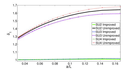
Figure 1: Comparison between unimproved and improved results for the fermionic contribution to the perturbative step scaling function for SU(2), SU(3) and SU(4) gauge theories with fundamental representation matter fields.

Next, in addition to using the coefficients in Table 1 the precise values of the boundary fields must be chosen carefully to guarantee rapid convergence of the results. In Fig. 2 we show the results for $\Sigma_{1,1}$ for SU(2) gauge theory and adjoint fermions. The results are normalized to the continuum values While the improvement is necessary to get rid of ${\cal{O}}(a)$ corrections, clearly, in order to guarantee that the ${\cal{O}}(a^{2})$ corrections remain small the boundary values must be optimized. The optimal choice is $\rho=\pi/2$ and $0<\eta<\pi/2$ excluding the value $\eta=\pi/4$. This can be understood as follows: If the boundary field is generically a diagonal matrix with eigenvalues $\phi$ and $-\phi$, then the adjoint fermions see these eigenvalues as $2\phi$, $-2\phi$ and 0. In other words, since the background appears twice as large for adjoint fermions as for fundamental fermions, it seems plausible that the problems could be alleviated by halving the background field. We note that the numerical results imply that with the above choice of parametrizing the boundary fields, the parameter $\rho$ plays the main role; i.e. there is a single value of $\rho$ (e.g. $\pi/2$ for the adjoint representation of SU(2)) for which the convergence is optimal and $\eta$ can be chosen from a wide interval without significantly altering the result.

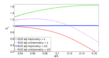
Figure 2: Comparison between two different boundary fields in SU(2) gauge theory with adjoint fermions. The thin solid and dashed curves correspond, respectively, to improved and unimproved results with $\rho=\pi$. The thick solid (dashed) curves correspond to improved (unimproved) results for $\rho=\pi/2$.

The analysis is straightforward also for SU(3) with higher representation fermions. In Fig. 3 we show $|\delta_{1}-1|$ contours in the $(\eta,\rho)$-plane. The conventional choice for the fundamental representation fermions is $(\rho,\eta)=(\pi/3,0)$. As in the case of SU(2), when translating the boundary matrix to the adjoint or sextet representation, one sees that the background field is effectively doubled. This again suggests trying to narrow the values of the angular parameters by a factor of two. This is indeed what we observe from Fig. 3: For the adjoint representation, shown in the upper panel, the best convergence of $\delta_{1}$ is obtained for $\rho=\pi/6$ and $-4\pi/9<\eta<\pi/9$ excluding the value $\eta=-\pi/6$. Similarly, as shown in the lower panel of the figure, for the sextet representation we find that the convergence is optimal for $\rho=67\pi/150\approx 0.45\pi$ and $-166\pi/225<-7\pi/45$ excluding $\eta=-67\pi/150$. As for SU(2), we find that the convergence is dominantly controlled by the value of the $\rho$ while $\eta$ can be chosen from a wide interval. For the figure we used $L/a=10$, but the results remain quantitatively similar for other values of $L/a$ as well; the dependence on $L/a$ is similar to the SU(2) case shown in Fig. 2.

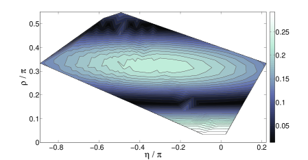
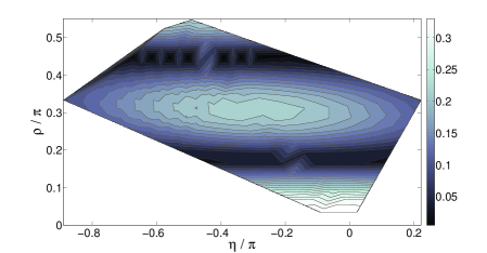
Figure 3: Convergence of $|\delta_{1}-1|$ as a function of $\rho$ and $\eta$ for adjoint (upper panel) and sextet (lower panel) fermions in SU(3) gauge theory.

Finally, the improvement coefficients must be included consistently. In Fig 4 we show comparison between the improved, unimproved results as well as between the results neglecting some of the improvement coefficients. In particular we see that even if the Sheikholeslami-Wohlert coefficient $c_{\rm{sw}}=1$ is implemented, but the boundary improvement is neglected, the results obtained under Schrödinger functional calculations like in DeGrand:2011qd are possibly still far from the proper continuum limit. Also the optimal values for the boundary fields used for the improved results in Fig. 4 differ from the values used for the fundamental representation as we discussed earlier. We have used here the values of $\rho$ and $\eta$ which give optimal convergence for $\delta_{1}$ as discussed in previous paragraphs.

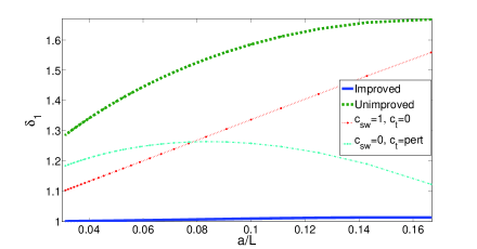
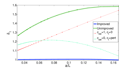
Figure 4: The upper panel shows the result for SU(3) with adjoint fermions and the lower one for SU(3) with sextet fermions. The thick solid and dashed curves correspond, respectively, to improved and unimproved results. The thin dotted (dash-dotted) curves correspond to the results obtained by setting $c_{\rm{sw}}=1\,(0)$ and $c_{t}=0$ (perturbative value).

In this Letter we have described developments in analyses of gauge theories with higher representation matter fields on the lattice. Generally, we have demonstrated the sensitivity of the results on the correct values of the improvement coefficients and boundary conditions when using Wilson fermions. We have provided perturbative values of the counterterm coefficients required for the analysis and emphasized the choice of the boundary conditions. Our results suggest that in studies of higher representations there is need to optimize the value of the background field carefully. This need is driven by the fermionic contribution; we have explicitly checked that the effect on the pure gauge contribution is negligible, on the level of few percents, for the cases we have considered.

- (1) H. Georgi, Phys. Rev. Lett. 98, 221601 (2007)
- (2) S. Weinberg, Phys. Rev. D 19, 1277 (1979); L. Susskind, Phys. Rev. D 20, 2619 (1979).
- (3) C. T. Hill and E. H. Simmons, Phys. Rept. 381, 235 (2003) [Erratum-ibid. 390, 553 (2004)] [arXiv:hep-ph/0203079].
- (4) F. Sannino, arXiv:0804.0182 [hep-ph].
- (5) T. Appelquist, A. Ratnaweera, J. Terning and L. C. R. Wijewardhana, Phys. Rev. D 58, 105017 (1998) [arXiv:hep-ph/9806472].
- (6) F. Sannino and K. Tuominen, Phys. Rev. D 71, 051901 (2005) [arXiv:hep-ph/0405209];
- (7) F. Bursa, L. Del Debbio, L. Keegan, C. Pica and T. Pickup, arXiv:1010.0901 [hep-ph]
- (8) T. Karavirta, J. Rantaharju, K. Rummukainen and K. Tuominen, arXiv:1111.4104 [hep-lat].
- (9) S. Catterall and F. Sannino, Phys. Rev. D 76, 034504 (2007) [arXiv:0705.1664 [hep-lat]].
- (10) A. J. Hietanen, J. Rantaharju, K. Rummukainen and K. Tuominen, JHEP 0905, 025 (2009) [arXiv:0812.1467 [hep-lat]]
- (11) L. Del Debbio, A. Patella and C. Pica, Phys. Rev. D 81 (2010) 094503 [arXiv:0805.2058 [hep-lat]].
- (12) S. Catterall, J. Giedt, F. Sannino and J. Schneible, arXiv:0807.0792 [hep-lat].
- (13) A. J. Hietanen, K. Rummukainen and K. Tuominen, Phys. Rev. D 80, 094504 (2009) [arXiv:0904.0864 [hep-lat]].
- (14) T. DeGrand, Y. Shamir, B. Svetitsky, [arXiv:1102.2843 [hep-lat]].
- (15) T. Appelquist, G. T. Fleming and E. T. Neil, Phys. Rev. Lett. 100, 171607 (2008) [arXiv:0712.0609 [hep-ph]].
- (16) Z. Fodor, K. Holland, J. Kuti, D. Nogradi and C. Schroeder, Phys. Lett. B 681, 353 (2009) [arXiv:0907.4562 [hep-lat]];
- (17) A. Deuzeman, M. P. Lombardo and E. Pallante, Phys. Lett. B 670, 41 (2008) [arXiv:0804.2905 [hep-lat]];
- (18) Y. Shamir, B. Svetitsky and T. DeGrand, Phys. Rev. D 78, 031502 (2008) [arXiv:0803.1707 [hep-lat]].
- (19) B. Sheikholeslami and R. Wohlert, Nucl. Phys. B 259 (1985) 572.
- (20) M. Luscher, R. Narayanan, P. Weisz and U. Wolff, Nucl. Phys. B 384, 168 (1992) [arXiv:hep-lat/9207009].
- (21) S. Sint and P. Vilaseca, arXiv:1111.2227 [hep-lat].
- (22) M. Luscher, R. Sommer, U. Wolff and P. Weisz, Nucl. Phys. B 389, 247 (1993) [hep-lat/9207010].
- (23) M. Luscher, R. Sommer, P. Weisz and U. Wolff, Nucl. Phys. B 413, 481 (1994) [arXiv:hep-lat/9309005].
- (24) S. Sint and R. Sommer, Nucl. Phys. B 465, 71 (1996) [arXiv:hep-lat/9508012].
- (25) R. Sommer, Nucl. Phys. Proc. Suppl. 60A, 279 (1998) [arXiv:hep-lat/9705026].
- (26) M. Luscher, S. Sint, R. Sommer and P. Weisz, Nucl. Phys. B 478, 365 (1996) [arXiv:hep-lat/9605038].
- (27) M. Luscher and P. Weisz, Nucl. Phys. B 479, 429 (1996) [arXiv:hep-lat/9606016].
- (28) T. Karavirta, A. Mykkanen, J. Rantaharju, K. Rummukainen and K. Tuominen, JHEP 1106, 061 (2011) [arXiv:1101.0154 [hep-lat]].