Outlook on the Higgs particles, masses and physical bounds in the Two Higgs-Doublet Model

Abstract

The Higgs sector of models beyond the standard model requires special attention and study, since through them, a natural explanation can be offered to current questions such as the big differences in the values of the masses of the quarks (hierarchy of masses), the possible generation of flavor changing neutral currents (inspired by the evidence about the oscillations of neutrinos), besides the possibility that some models, with more complicated symmetries than those of the standard model, have a non standard low energy limit. The simplest extension of the standard model known as the two-Higgs-doublet-model (2HDM) involves a second Higgs doublet. The 2HDM predicts the existence of five scalar particles: three neutral ($A^{0}$), ($h^{0}$, $H^{0}$) and two charged ($H^{\pm}$). The purpose of this work is to determine in a natural and easy way the mass eigenstates and masses of these five particles, in terms of the parameters $\lambda_{i}$ introduced in the minimal extended Higgs sector potential that preserves the CP symmetry. We discuss several cases of Higgs mixings and the one in which two neutral states are degenerate. As the values of the quartic interactions between the scalar doublets are not theoretically determined, it is of great interest to explore and constrain their values, therefore we analize the stability and triviality bounds using the Lagrange multipliers method and numerically solving the renormalization group equations. Through the former results one can establish the region of validity of the model under several circumstances considered in the literature.

I Introduction

The Standard Model (SM) in high energy physics wsg has been remarkably successful in: describing the properties of elementary particles, predicting the existence of the quarks $c$, $t$ and $b$, and the third generation of leptons $\tau$- $\nu_{\tau}$, the existence of the eight gluons, and the weak bosons $W^{\pm}$, $Z^{0}$ before their discovery, predicting parity violating neutral-weak-currents, and in being consistent with all the experimental results PDG ; CERN . However, the SM falls short of being a complete theory of the fundamental interactions because of its lack of explanation of the probable unification of the fundamental interactions, the pattern and disparity of the particle masses (mass hierarchy), the origin of the CP violation in nature, the matter-antimatter asymmetry, the pattern of quark mixing, lepton mixing and the reason why there are 3 generations.

As a partial solution to confront these deficiencies, a large number of parameters must be put in “by hand” into the theory (rather than being derived from first principles), such as the three gauge couplings ($g_{1}$, $g_{2}$ and $g_{3})$, nine fermionic masses (six quarks and three leptons), the Weinberg angle ($\theta_{w}$), four quark-mixing parameters (CKM) and two more parameters in relation to the Higgs potential ($\mu$ and $\lambda$).

One of the most subtle aspects of the model is associated with the Higgs sector Higgs . The Higgs field and its non-vanishing vacuum expectation value (vev) is the essential ingredient to carry out the spontaneous symmetry breaking (SSB) required to transform the hypothetical massless particles in the Lagrangian into the actual massive physical particles. However, the Higgs particle has not yet been discovered.

In this paper we study the extension of the SM with two Higgs doublets (2HDM) that presents the challenge that the quartic interactions between the scalar doublets are not theoretically determined. This model is studied mainly for three reasons. The first one is that the 2HDM has a much richer Higgs spectrum (3 neutral and 2 charged Higgses) and a different high energy behavior. This makes that a lower mass than in the SM Higgs is permitted. Another reason may be that a different pattern of hierarchy of the Yukawa couplings is possible, because of the presence of two independent vacuum expectation values of the Higgs fields . The third reason is that the Higgs sector of the Minimal Supersymmetric Standard Model (MSSM) contains two Higgs doublets, so the Higgs sectors of the MSSM and the 2HDM are similar and the study of the 2HDM model may give important information on the properties of the Higgs sector in the MSSM .

In Section II we introduce the potential for the 2HDM in a special parametrization, and briefly discuss the SSB. In Sections III and IV we present the Higgs mass matrix and its diagonalization method, the mass spectrum, mass eigestates, and special cases of mixing, where the Higgs masses are simply related to the parameters of the potential. In Section V we obtain and classify the constrains for the quartic couplings derived from the mass formulas, from the vacuum stability principle through the Lagrange multipliers method, and by imposing extreme stability conditions. In Section VI we numerically solve the set of the renormalization group equations from which through triviality principle the physical bounds of the model are determined under different conditions. Finally, Section VII is devoted to the presentation of the results and the conclusions.

II The two-Higgs doublet model

In the SM the fermion masses arise, after the SSB, from the couplings between the fermions and a single Higgs doublet. The mass ratio of the $b$ and $t$ quark is of the order of $1/40.$ To understand in a natural way the origin of this difference in the values of the masses of the third generation of quarks, one can assume the existence of a second Higgs-doublet in the Higgs sector of the SM. In this context one assumes that the quark $t$ obtains its mass through the $\Phi_{1}$ doublet and the quark $b$ from another doublet $\Phi_{2}$ . In this way one can explain in a more natural way the hierarchy problem of the Yukawa couplings, as long as the free parameters of the new model acquire the appropriate values.

The Higgs sector of the 2HDM consists of two identical (hypercharge-one) scalar doublets $\Phi_{1}$ and $\Phi_{2}$. There are several proposals for the Higgs potential to describe the physical reality in the framework of the 2HDM Inoue ; GHKD . The potential we consider in this paper is compatible with Ref. Kominis . It is such that the CP symmetry (charge-conjugation and parity) is conserved, the neutral-Higgs-mediated flavor-changing neutral currents (FCNC) are suppressed in the leptonic sector, and in the quark-sector they are also forbidden by the GIM mechanism GIM in the one loop approximation. In the Lagrangian $\mathcal{L}$ in which we leave out the leptonic terms,

$$\mathcal{L=L}_{gf}+\mathcal{L}_{Kin}+\mathcal{L}_{Y}-V$$ (1)

the $\mathcal{L}_{gf}$ and $\mathcal{L}_{Kin}$ correspond to kinetic parts of quarks and bosons and they contain the covariant derivatives that provide the interactions among the gauge bosons and the Higgs bosons. They also give rise, after the SSB, to the masses of the gauge bosons (mediators of the electroweak interactions). The fermion masses are generated from the Yukawa couplings in $\mathcal{L}_{Y}$

$$\mathcal{L}_{Y}=\sum_{i.j}\left(g_{ij}^{(u)}\overline{\psi}_{Li}\Phi_{1}^{c}u_{Rj}+g_{ij}^{(d)}\overline{\psi}_{Li}\Phi_{2}d_{Rj}\right),$$ (2)

between the Higgs bosons and the quarks. In $\mathcal{L}_{Y}$, the $g_{ij}^{(u,d)}$ are the Yukawa coupling matrices. The superscripts $(u,d)$ refer to the up and down sectors of quarks, respectively and the subscripts $\left(L,R\right)$ correspond to the left handed doublets and right handed singlets in the quark sector. In this paper, we will focus our attention on the potential $V$.

The Higgs potential

The Higgs potential depends on seven real parameters $\mu_{1}^{2},\mu_{2}^{2}$ and $\lambda_{i\,}\,\,(i=1...,5)$ from which the five Higgs masses come up after the SSB. The most general renormalizable $SU(2)\times U(1)$ invariant Higgs potential, that preserves a CP and a Z₂ symmetry ($\Phi_{1}\rightarrow\Phi_{1},\,\,\Phi_{2}\rightarrow-\Phi_{2})$ is given by

$$V=\mu_{1}^{2}\Phi_{1}^{\dagger}\Phi_{1}+\mu_{2}^{2}\Phi_{2}^{\dagger}\Phi_{2}+\lambda_{1}\left(\Phi_{1}^{\dagger}\Phi_{1}\right)^{2}+\lambda_{2}\left(\Phi_{2}^{\dagger}\Phi_{2}\right)^{2}+\lambda_{3}\left(\Phi_{1}^{\dagger}\Phi_{1}\right)\left(\Phi_{2}^{\dagger}\Phi_{2}\right)\\ +\lambda_{4}\left(\Phi_{1}^{\dagger}\Phi_{2}\right)\left(\Phi_{2}^{\dagger}\Phi_{1}\right)+\frac{1}{2}\lambda_{5}\left[\left(\Phi_{1}^{\dagger}\Phi_{2}\right)^{2}+\left(\Phi_{2}^{\dagger}\Phi_{1}\right)^{2}\right].$$ (3)

For the sake of simplicity a special basis is introduced

$$A=\Phi_{1}^{\dagger}\Phi_{1},\quad B=\Phi_{2}^{\dagger}\Phi_{2},\quad C^{\prime}=D^{{\prime}{\dagger}}=\Phi_{1}^{\dagger}\Phi_{2}.$$ (4)

In this basis

$$V=\mu_{1}^{2}A+\mu_{2}^{2}B+\lambda_{1}A^{2}+\lambda_{2}B^{2}+\lambda_{3}AB+\lambda_{4}C^{\prime}D^{\prime}+\frac{1}{2}\lambda_{5}\left[C^{\prime 2}+D^{\prime 2}\right].$$ (5)

The two Higgs doublets can be represented by eight real fields $\phi_{i},\,i=1,\ldots,8$,

$$\Phi_{1}=\left(\begin{array}[]{l}\phi_{1}+i\phi_{2}\\ \phi_{3}+i\phi_{4}\end{array}\right),\quad\Phi_{2}=\left(\begin{array}[]{l}\phi_{5}+i\phi_{6}\\ \phi_{7}+i\phi_{8}\end{array}\right).\,$$ (6)

If charge is conserved and there is no CP violation in the Higgs sector, after the SSB, the non-vanishing vacuum expectation values of the fields $\phi_{3}$ and $\phi_{7}$ are real,

$$\left\langle\phi_{3}\right\rangle=\frac{v_{1}}{\sqrt{2}},\quad\left\langle\phi_{7}\right\rangle=\frac{v_{2}}{\sqrt{2}},$$ (7)

$$\left\langle\phi_{1}\right\rangle=\left\langle\phi_{2}\right\rangle=\left\langle\phi_{4}\right\rangle=0,\quad\left\langle\phi_{5}\right\rangle=\left\langle\phi_{6}\right\rangle=\left\langle\phi_{8}\right\rangle=0.$$ (8)

In terms of the fields $\phi_{i},$ the hermitian basis is given by

$$\begin{split}A&=\phi_{1}^{2}+\phi_{2}^{2}+\phi_{3}^{2}+\phi_{4}^{2},\quad B=\phi_{5}^{2}+\phi_{6}^{2}+\phi_{7}^{2}+\phi_{8}^{2},\\ C^{\prime}&=\phi_{1}\phi_{5}+i\phi_{1}\phi_{6}-i\phi_{2}\phi_{5}+\phi_{2}\phi_{6}+\phi_{3}\phi_{7}+i\phi_{3}\phi_{8}-i\phi_{4}\phi_{7}+\phi_{4}\phi_{8},\\ D^{\prime}&=\phi_{1}\phi_{5}+i\phi_{2}\phi_{5}-i\phi_{1}\phi_{6}+\phi_{2}\phi_{6}+\phi_{3}\phi_{7}+i\phi_{4}\phi_{7}-i\phi_{3}\phi_{8}+\phi_{4}\phi_{8}.\end{split}$$ (9)

and after the SSB they become

$$\left\langle A\right\rangle=\frac{1}{2}v_{1}^{2},\quad\left\langle B\right\rangle=\frac{1}{2}v_{2}^{2},\quad\left\langle C^{\prime}\right\rangle=\left\langle D^{\prime}\right\rangle=\frac{1}{2}v_{1}v_{2}.$$ (10)

III The mass matrix

The conditions for the minimum of the potential are obtained from the vanishing of the first derivatives at the minimum $\left.\frac{\partial V}{\partial\phi_{i}}\right|_{\min}=0$, with the condition that the matrix of the second derivatives at the minimum: $\left.\frac{\partial^{2}V}{\partial\phi_{i}\partial\phi_{j}}\right|_{\min}$ is positive definite. Therefore

$$\left.\frac{\partial V}{\partial\phi_{i}}\right|_{\left\langle 0\right|\phi_{i}\left|0\right\rangle}=\left\langle 0\right|\mu_{1}^{2}\frac{\partial}{\partial\phi_{i}}A+\mu_{2}^{2}\frac{\partial}{\partial\phi_{i}}B+2\lambda_{1}A\frac{\partial}{\partial\phi_{i}}A+2\lambda_{2}B\frac{\partial}{\partial\phi_{i}}B+\lambda_{3}B\frac{\partial A}{\partial\phi_{i}}+\lambda_{3}A\frac{\partial B}{\partial\phi_{i}}\\ +\lambda_{4}D^{\prime}\frac{\partial C^{\prime}}{\partial\phi_{i}}+\lambda_{4}C^{\prime}\frac{\partial D^{\prime}}{\partial\phi_{i}}+\lambda_{5}\left[C^{\prime}\frac{\partial}{\partial\phi_{i}}C^{\prime}+D^{\prime}\frac{\partial}{\partial\phi_{i}}D^{\prime}\right]\left|0\right\rangle=0$$ (11)

from which after some simplifications two non trivial equations are obtained

$$\mu_{1}^{2}+\lambda_{1}v_{1}^{2}+2\lambda_{T}\,v_{2}^{2}=0\;\text{ or }\;v_{1}=0,\quad\mu_{2}^{2}+\lambda_{2}v_{2}^{2}+2\lambda_{T}v_{1}^{2}=0\;\text{ or }\;v_{2}=0,$$ (12)

where

$$\lambda_{T}\equiv\left(\lambda_{3}+\lambda_{4}+\lambda_{5}\right).$$ (13)

The mass matrix elements are obtained from the equation

$$M_{ij}^{2}=\frac{1}{2}\left.\frac{\partial^{2}V}{\partial\phi_{i}\partial\phi_{j}}\right|_{\phi_{3}=\frac{v_{1}}{\sqrt{2}},\phi_{7}=\frac{v_{2}}{\sqrt{2}}},$$ (14)

and the explicit form of the matrix of the second derivatives reads

$$\frac{\partial^{2}V}{\partial\phi_{j}\partial\phi_{i}}=\left(\mu_{1}^{2}+2\lambda_{1}A+\lambda_{3}B\right)\frac{\partial^{2}A}{\partial\phi_{j}\partial\phi_{i}}+\left(\mu_{2}^{2}+2\lambda_{2}B+\lambda_{3}A\right)\frac{\partial^{2}B}{\partial\phi_{j}\partial\phi_{i}}+2\lambda_{1}\frac{\partial A}{\partial\phi_{j}}\frac{\partial A}{\partial\phi_{i}}+2\lambda_{2}\frac{\partial B}{\partial\phi_{j}}\frac{\partial B}{\partial\phi_{i}}\\ +\lambda_{3}\left(\frac{\partial A}{\partial\phi_{j}}\frac{\partial B}{\partial\phi_{i}}+\frac{\partial B}{\partial\phi_{j}}\frac{\partial A}{\partial\phi_{i}}\right)+\lambda_{5}\left(\frac{\partial C^{\prime}}{\partial\phi_{j}}\frac{\partial C^{\prime}}{\partial\phi_{i}}+\frac{\partial D^{\prime}}{\partial\phi_{j}}\frac{\partial D^{\prime}}{\partial\phi_{i}}\right)+\lambda_{4}\left(\frac{\partial C^{\prime}}{\partial\phi_{j}}\frac{\partial D^{\prime}}{\partial\phi_{i}}+\frac{\partial D^{\prime}}{\partial\phi_{j}}\frac{\partial C^{\prime}}{\partial\phi_{i}}\right)\\ +\left(\lambda_{4}D^{\prime}+\lambda_{5}C^{\prime}\right)\frac{\partial^{2}C^{\prime}}{\partial\phi_{j}\partial\phi_{i}}+\left(\lambda_{4}C^{\prime}+\lambda_{5}D^{\prime}\right)\frac{\partial^{2}D^{\prime}}{\partial\phi_{j}\partial\phi_{i}}.$$ (15)

Using Eqs. (12) the 16 non vanishing matrix elements are

$$\begin{split}M_{11}^{2}&=M_{22}^{2}=-\frac{1}{2}\left(\lambda_{4}+\lambda_{5}\right)v_{2}^{2},\quad M_{33}^{2}=2\lambda_{1}v_{1}^{2},\quad M_{44}^{2}=-\lambda_{5}v_{2}^{2},\\ M_{55}^{2}&=M_{66}^{2}=-\frac{1}{2}\left(\lambda_{4}+\lambda_{5}\right)v_{1}^{2},\quad M_{77}^{2}=2\lambda_{2}v_{2}^{2},\quad M_{88}^{2}=-\lambda_{5}v_{1}^{2},\\ M_{15}^{2}&=M_{51}^{2}=M_{26}^{2}=M_{62}^{2}=\frac{1}{2}\left(\lambda_{4}+\lambda_{5}\right)v_{1}v_{2},\\ M_{37}^{2}&=M_{73}^{2}=\left(\lambda_{3}+\lambda_{4}+\lambda_{5}\right)v_{1}v_{2},\quad M_{48}^{2}=M_{84}^{2}=\lambda_{5}v_{1}v_{2}.\end{split}$$ (16)

Diagonalization of the mass matrix

The Higgs masses and the Higgs mass-eigenstates are obtained after a suitable diagonalization of the matrix in Eq. (14). The diagonalization of the matrix whose elements are given in Eq. (16) is performed in two steps.

A block ordering is performed and a diagonalization of each block is carried out. The blocks are obtained by means of the application of two consecutive unitary transformations $U_{1}=U_{1}^{\dagger}$ and $U_{2}=U_{2}^{\dagger}$

$$\left(M_{ij}^{2}\right)_{B}=U_{2}U_{1}M_{ij}^{2}U_{1}^{\dagger}U_{2}^{\dagger}.$$ (17)

The non vanishing matrix elements of the unitary transformations are

$$\left(U_{1}\right)_{11}=\left(U_{1}\right)_{25}=\left(U_{1}\right)_{33}=\left(U_{1}\right)_{44}=\left(U_{1}\right)_{52}=\left(U_{1}\right)_{66}=\left(U_{1}\right)_{77}=\left(U_{1}\right)_{88}=1,$$

$$\left(U_{2}\right)_{11}=\left(U_{2}\right)_{22}=\left(U_{2}\right)_{33}=\left(U_{2}\right)_{47}=\left(U_{2}\right)_{55}=\left(U_{2}\right)_{66}=\left(U_{2}\right)_{74}=\left(U_{2}\right)_{88}=1.$$

After carrying out both transformations, the $8\times 8$ matrix becomes

$$\left(M_{ij}^{2}\right)_{B}=\left(\begin{array}[]{llllllll}M_{11}^{2}&M_{15}^{2}&0&0&0&0&0&0\\ M_{51}^{2}&M_{55}^{2}&0&0&0&0&0&0\\ 0&0&M_{33}^{2}&M_{37}^{2}&0&0&0&0\\ 0&0&M_{73}^{2}&M_{77}^{2}&0&0&0&0\\ 0&0&0&0&M_{22}^{2}&M_{26}^{2}&0&0\\ 0&0&0&0&M_{62}^{2}&M_{66}^{2}&0&0\\ 0&0&0&0&0&0&M_{44}^{2}&M_{48}^{2}\\ 0&0&0&0&0&0&M_{84}^{2}&M_{88}^{2}\end{array}\right).$$ (18)

The matrix in Eq. (18), is ready to easily perform the total diagonalization

$$\left(M_{ij}^{2}\right)_{B}=\left(\begin{array}[]{ll}M_{11}^{2}&M_{15}^{2}\\ M_{51}^{2}&M_{55}^{2}\end{array}\right)\oplus\left(\begin{array}[]{ll}M_{33}^{2}&M_{37}^{2}\\ M_{73}^{2}&M_{77}^{2}\end{array}\right)\oplus\left(\begin{array}[]{ll}M_{22}^{2}&M_{26}^{2}\\ M_{62}^{2}&M_{66}^{2}\end{array}\right)\oplus\left(\begin{array}[]{ll}M_{44}^{2}&M_{48}^{2}\\ M_{84}^{2}&M_{88}^{2}\end{array}\right).$$ (19)

The next step is to perform the diagonalization of each of the submatrices in Eq. (19).

IV Higgs mass-eigenstates basis

Let us now proceed to relate the gauge states with the mass eigenstates.

The scalar fields in Eq. (6) can be represented as

$$\Phi_{1}=\left(\begin{array}[]{l}\phi_{1}^{+}\\ \phi_{1}^{0}\end{array}\right);\,\,\,\,\Phi_{2}=\left(\begin{array}[]{l}\phi_{2}^{+}\\ \phi_{2}^{0}\end{array}\right)$$ (20)

where

$$\phi_{1}^{+}=\phi_{1}+i\phi_{2},\quad\phi_{2}^{+}=\phi_{5}+i\phi_{6},\quad\phi_{1}^{0}=\phi_{3}+i\phi_{4},\quad\phi_{2}^{0}=\phi_{7}+i\phi_{8},$$ (21)

and

$$\phi_{3}=\frac{v_{1}}{\sqrt{2}}+h_{1},\,\;\phi_{4}=\eta_{1},\quad\phi_{7}=\frac{v_{2}}{\sqrt{2}}+h_{2},\quad\phi_{8}=\eta_{2}.$$ (22)

Now, the physical fields (mass eigenstates) and the Goldstones (massless eigenstates) are obtained from the gauge eigenstates by a unitary transformation that diagonalizes the corresponding submatrices Eq. (19), in the following way

$$\left(\begin{array}[]{l}H^{0}\\ h^{0}\end{array}\right)=U_{\alpha}\left(\begin{array}[]{l}h_{1}\\ h_{2}\end{array}\right),\quad\left(\begin{array}[]{l}G^{+}\\ H^{+}\end{array}\right)=U_{\beta}\left(\begin{array}[]{l}\phi_{1}^{+}\\ \phi_{2}^{+}\end{array}\right),\quad\left(\begin{array}[]{l}G^{0}\\ A^{0}\end{array}\right)=U_{\gamma}\left(\begin{array}[]{l}\eta_{1}\\ \eta_{2}\end{array}\right),$$ (23)

where

$$U_{\alpha}=\left(\begin{array}[]{cc}\cos\alpha&\sin\alpha\\ -\sin\alpha&\cos\alpha\end{array}\right),\quad U_{\alpha}^{\dagger}U_{\alpha}=I$$ (24)

and $U_{\beta}=U_{\gamma}$ have the same form as $U_{\alpha}$. $\alpha$ is the mixing angle between the neutral states $\phi_{1}^{0}$ and $\phi_{2}^{0}$, i.e., $\phi_{3}$ and $\phi_{7}$ , the $\beta$ angle is the one between the charged states, and $\gamma$ is related with the CP-Odd states $\phi_{4}$ and $\phi_{8}$.

$$\tan\alpha=\frac{y}{1+\sqrt{1+y^{2}}},\quad y=\tan 2\alpha=\frac{\left(\lambda_{3}+\lambda_{4}+\lambda_{5}\right)v_{1}v_{2}}{\left(\lambda_{1}v_{1}^{2}-\lambda_{2}v_{2}^{2}\right)},\quad-\frac{\pi}{2}<\alpha<\frac{\pi}{2},$$ (25)

and

$$\tan\beta=\frac{v_{2}}{v_{1}},\quad v^{2}=\left(v_{1}^{2}+v_{2}^{2}\right),\quad 0<\beta<\frac{\pi}{2},\quad\gamma=\beta.$$ (26)

The resulting physical particles in the Higgs-sector are: two CP-even-neutral Higgs scalars ($H^{0},h^{0}$), one CP-odd neutral Higgs scalar ($A^{0}$), two charged Higgs bosons ($H^{\pm}$), and three Goldstone-bosons ($G^{\pm},G^{0}$) that contribute to the mass generation of the gauge vector bosons $W^{\pm}$ and $Z^{0}$, respectively.

The mass formulas

After the complete diagonalization, we obtain the following relations:

1. The mass eigenvalues for ($H^{0},h^{0}$) are

   $$M_{H^{0},h^{0}}^{2}=\lambda_{1}v_{1}^{2}+\lambda_{2}v_{2}^{2}\pm\sqrt{\left(\lambda_{1}v_{1}^{2}-\lambda_{2}v_{2}^{2}\right)^{2}+\left(v_{1}v_{2}\lambda_{T}\right)^{2}}>0,$$ (27)

2. The eigenvalues for the mass eigenstates $H^{\pm}$ and $G^{\pm}$ are

   $$M_{G^{\pm}}^{2}=0\;,\quad M_{H^{\pm}}^{2}=-\frac{1}{2}\left(\lambda_{4}+\lambda_{5}\right)v^{2}>0,$$ (28)

3. Finally, the mass eigenvalues for $G^{0}$ and $A^{0}$ are

   $$M_{G^{0}}^{2}=0,\quad M_{A^{0}}^{2}=-\lambda_{5}v^{2}>0,$$ (29)

As expected, after the electroweak symmetry breaking (EWSB) the eight components of the two complex isodoublet fields are transformed into: two charged Higgs bosons $H^{\pm}$, three neutral Higgs bosons $H^{0},h^{0},A^{0}$, and three massless Goldstone fields $G^{0},G^{\pm}$ (which are transformed into the longitudinal components of the gauge bosons $W^{\pm}$ and $Z^{0}$). At this level, the values of $M_{A^{0}}$ and $M_{H^{\pm}}$ are not related to the parameters $\lambda_{1}$, $\lambda_{2}$ and $\lambda_{3}$. This means that, apparently, there is a complete independence between the $A^{0}$, $H^{\pm}$ and the $h^{0}$, $H^{0}$, which is not all true.
As in the Standard Model, the values of the quartic couplings are not fixed by the model. To proceed as in the SM KJ , to determine the Higgs masses, one has to consider two important physical principles. The vacuum stability constrains the values for the quartic couplings. To have a complete view, we invert the former equations to express the quartic parameters in terms of the masses of the Higgs fields.

$$\lambda_{1}=\frac{1}{2v_{1}^{2}}\left(M_{H^{0}}^{2}\cos^{2}\alpha+M_{h^{0}}^{2}\sin^{2}\alpha\right),\quad\lambda_{2}=\frac{1}{2v_{2}^{2}}\left(M_{H^{0}}^{2}\sin^{2}\alpha+M_{h^{0}}^{2}\cos^{2}\alpha\right)$$ (30)

$$\lambda_{3}=\frac{\left(M_{H^{0}}^{2}-M_{h^{0}}^{2}\right)}{2v_{1}v_{2}}\sin 2\alpha+2\frac{M_{H^{\pm}}^{2}}{v^{2}},\quad\lambda_{4}=\frac{M_{A^{0}}^{2}-2M_{H^{\pm}}^{2}}{v^{2}}\quad\lambda_{5}=-\frac{M_{A^{0}}^{2}}{v^{2}},$$ (31)

$$\lambda_{T}=\left(\lambda_{3}+\lambda_{4}+\lambda_{5}\right)=\frac{\left(M_{H^{0}}^{2}-M_{h^{0}}^{2}\right)}{2v_{1}v_{2}}\sin 2\alpha.$$ (32)

Particular cases

To obtain Eq. (30)-(32) we have considered the following relations: Since Eq. (27) is equivalent to

$$M_{H^{0},h^{0}}^{2}=\left[\lambda_{1}v_{1}^{2}+\lambda_{2}v_{2}^{2}\pm\left(\lambda_{1}v_{1}^{2}-\lambda_{2}v_{2}^{2}\right)\sqrt{1+y^{2}}\right]$$ (33)

and

$$\sqrt{1+y^{2}}=\sqrt{1+\left(\tan 2\alpha\right)^{2}}=\frac{1}{\cos 2\alpha},$$ (34)

we obtain from Eq. (25)

$$\sin 2\alpha=\frac{\left(\lambda_{3}+\lambda_{4}+\lambda_{5}\right)v_{1}v_{2}}{\sqrt{\left(\lambda_{1}v_{1}^{2}-\lambda_{2}v_{2}^{2}\right)^{2}+\left(\lambda_{3}+\lambda_{4}+\lambda_{5}\right)^{2}\left(v_{1}v_{2}\right)^{2}}}$$ (35)

as well as

$$\cos 2\alpha=\frac{\lambda_{1}v_{1}^{2}-\lambda_{2}v_{2}^{2}}{\sqrt{\left(\lambda_{1}v_{1}^{2}-\lambda_{2}v_{2}^{2}\right)^{2}+\left(\lambda_{3}+\lambda_{4}+\lambda_{5}\right)^{2}\left(v_{1}v_{2}\right)^{2}}}$$ (36)

and

$$\frac{\left(M_{H^{0}}^{2}-M_{h^{0}}^{2}\right)\cos 2\alpha}{2}=\left(\lambda_{1}v_{1}^{2}-\lambda_{2}v_{2}^{2}\right),\quad\,\frac{M_{H^{0}}^{2}+M_{h^{0}}^{2}}{2}=\left[\lambda_{1}v_{1}^{2}+\lambda_{2}v_{2}^{2}\right].$$ (37)

With these equations it is easy to obtain Eq. (30).
a.- In the case when the mixing angle is $\alpha=0$, i.e., $\lambda_{T}=0$, $\lambda_{3}>0$,

$$\lambda_{1}=\frac{1}{2v_{1}^{2}}M_{H^{0}}^{2},\quad\lambda_{2}=\frac{1}{2v_{2}^{2}}M_{h^{0}}^{2},\quad\lambda_{3}=2\left(\frac{M_{H^{\pm}}}{v}\right)^{2},$$ (38)

$$\lambda_{4}=\left(\frac{M_{A^{0}}}{v}\right)^{2}-2\left(\frac{M_{H^{\pm}}}{v}\right)^{2},\quad\lambda_{5}=-\left(\frac{M_{A^{0}}}{v}\right)^{2},$$ (39)

and

$$M_{H^{0}}^{2}-M_{h^{0}}^{2}=2\left(\lambda_{1}v_{1}^{2}-\lambda_{2}v_{2}^{2}\right).$$ (40)

The parameters $\mu_{1},\mu_{2}$ in the potential Eq. (3) are related to the neutral Higgs particles in a very simple way, similar to the one between the parameters $\lambda$ and $\mu$ in the SM.

$$-2\mu_{1}^{2}=M_{H^{0}}^{2}=2\lambda_{1}v_{1}^{2},\quad-2\mu_{2}^{2}=M_{h^{0}}^{2}=2\lambda_{2}v_{2}^{2}.$$ (41)

and the vevs satisfy

$$v^{2}=\left(v_{1}^{2}+v_{2}^{2}\right)=-\left(\frac{\mu_{2}^{2}}{\lambda_{2}}+\frac{\mu_{1}^{2}}{\lambda_{1}}\right)=\frac{1}{2\lambda_{1}\lambda_{2}}\left(\lambda_{1}M_{h^{0}}^{2}+\lambda_{2}M_{H^{0}}^{2}\right).$$ (42)

In this particular case, each Higgs particle is associated with a specific parameter $\lambda_{1}$, $\lambda_{2}$, $\lambda_{3}$, $\lambda_{5}$.

$$M_{H^{0}}=v_{1}\sqrt{2\lambda_{1}},\quad M_{h^{0}}=v_{2}\sqrt{2\lambda_{2}},\quad M_{H^{\pm}}=\frac{v}{\sqrt{2}}\sqrt{\lambda_{3}},\quad M_{A^{0}}=v\sqrt{\left|\lambda_{5}\right|}.$$ (43)

The degeneracy in the masses $M_{H^{0}}$, $M_{h^{0}}$ implies that $\lambda_{1}v_{1}^{2}-\lambda_{2}v_{2}^{2}=0$.
b.- In the case when the mixing angle is $\alpha=\pi/2$, $\lambda_{T}=0$

$$\lambda_{1}=\frac{1}{2v_{1}^{2}}M_{h^{0}}^{2},\quad\lambda_{2}=\frac{1}{2v_{2}^{2}}M_{H^{0}}^{2},\quad\lambda_{3}=2\left(\frac{M_{H^{\pm}}}{v}\right)^{2},$$ (44)

$$\lambda_{4}=\left(\frac{M_{A^{0}}}{v}\right)^{2}-2\left(\frac{M_{H^{\pm}}}{v}\right)^{2},\quad\lambda_{5}=-\left(\frac{M_{A^{0}}}{v}\right)^{2}.$$ (45)

The parameters $\mu_{1},\mu_{2}$ in Eq. (12) become:

$$-2\mu_{1}^{2}=M_{h^{0}}^{2}=2\lambda_{1}v_{1}^{2},\quad-2\mu_{2}^{2}=M_{H^{0}}^{2}=2\lambda_{2}v_{2}^{2}.$$ (46)

and

$$v^{2}=\frac{1}{2\lambda_{1}\lambda_{2}}\left(\lambda_{1}M_{H^{0}}^{2}+\lambda_{2}M_{h^{0}}^{2}\right).$$ (47)

As in the former case, each Higgs particle is associated with a specific parameter $\lambda_{i}$, and ($H^{0},h^{0}$) interchange places.

$$M_{h^{0}}=v_{1}\sqrt{2\lambda_{1}},\quad M_{H^{0}}=v_{2}\sqrt{2\lambda_{2}},\quad M_{H^{\pm}}=\frac{v}{\sqrt{2}}\sqrt{\lambda_{3}},\quad M_{A^{0}}=v\sqrt{\left|\lambda_{5}\right|}.$$ (48)

In this section, we have considered the main features of various special cases for the parameter $\alpha$ where a decoupling of the Higgs bosons take place, and the case where the masses of the CP-even neutral particles coincide.

V Vacuum stability constrains

Bounds due to the positive mass-values

Due to the fact that the masses are positive, from the previous results, one gets information for the allowed values of the $\lambda_{i}$ parameters.

$$\lambda_{1}>0,\quad\lambda_{2}>0,\quad\left(\lambda_{4}+\lambda_{5}\right)<0,\ \ \lambda_{5}<0,\ \ \lambda_{4}<\left|\lambda_{5}\right|.$$ (49)

and Eq. (27) implies that

$$\lambda_{1}\lambda_{2}>\frac{1}{4}\left(\lambda_{3}+\lambda_{4}+\lambda_{5}\right)^{2}.$$ (50)

In terms of the masses, the conditions in Eq. (49) and Eq. (50) become trivial

$$\lambda_{1}=\frac{1}{2v_{1}^{2}}\left[M_{H^{0}}^{2}\cos^{2}\alpha+M_{h^{0}}^{2}\sin^{2}\alpha\right]>0,$$ (51)

$$\lambda_{2}=\frac{1}{2v_{2}^{2}}\left[M_{H^{0}}^{2}\sin^{2}\alpha+M_{h^{0}}^{2}\cos^{2}\alpha\right]>0,$$ (52)

$$\lambda_{1}\lambda_{2}-\frac{1}{4}\left(\lambda_{3}+\lambda_{4}+\lambda_{5}\right)^{2}=\frac{1}{4v_{1}^{2}v_{2}^{2}}M_{H^{0}}^{2}M_{h^{0}}^{2}>0.$$ (53)

To improve previous information about the allowed values of the quartic couplings and therefore for the masses, we have explored the consecuences of considering the vacuum stability conditions (VSC), through the method of the Lagrange multipliers.

Lagrangian multipliers method and the VSC

Considering one restriction: Let us introduce the variables $x_{i}$ and the parameters $b_{i}$, defined as 

$$x_{1}=\left|\Phi_{1}\right|^{2},\quad x_{2}=\left|\Phi_{2}\right|^{2},\,\,x_{3}=\frac{1}{2}\left(\Phi_{1}^{\dagger}\Phi_{2}+\Phi_{2}^{\dagger}\Phi_{1}\right),\,\,\,\,x_{4}=\frac{1}{2i}\left(\Phi_{1}^{\dagger}\Phi_{2}-\Phi_{2}^{\dagger}\Phi_{1}\right),$$ (54)

$$b_{11}=\lambda_{1},\quad b_{22}=\lambda_{2},\quad b_{33}=\left(\lambda_{4}+\lambda_{5}\right),\quad b_{44}=\left(\lambda_{4}-\lambda_{5}\right),\quad b_{12}=\lambda_{3},$$ (55)

the potential in Eq. (3) becomes $V=V_{0}+x_{1}^{2}F_{0},$ where $V_{0}=\mu_{1}^{2}x_{1}+\mu_{2}^{2}x_{2}$, and

$$F_{0}=b_{11}+b_{12}\xi_{2}+b_{22}\xi_{2}^{2}+b_{33}\xi_{3}^{2}+b_{44}\xi_{4}^{2},\quad\xi_{i}=\frac{x_{i}}{x_{1}},\;i=2,3,4.$$ (56)

Using the Cauchy-Scwartz inequality

$$\left|\Phi_{1}^{\dagger}\Phi_{2}\right|^{2}\leq\Phi_{1}^{\dagger}\Phi_{1}\Phi_{2}^{\dagger}\Phi_{2}=\left|\Phi_{1}\right|^{2}\left|\Phi_{2}\right|^{2},$$ (57)

we obtain the condition

$$f\left(\xi_{2},\xi_{3},\xi_{4}\right)=\xi_{3}^{2}+\xi_{4}^{2}-\xi_{2}\leq 0.$$ (58)

We now introduce the Lagrange multiplier $\Lambda_{1}$ in the quartic sector of the potential  related to the condition imposed by the Cauchy-Schwarz inequality Eq. (58)

$$F\left(\xi_{2},\xi_{3},\xi_{4},\Lambda_{1}\right)=F_{0}\left(\xi_{2},\xi_{3},\xi_{4}\right)+\Lambda_{1}\,f\left(\xi_{2},\xi_{3},\xi_{4}\right)=b_{11}+\left(b_{12}-\Lambda_{1}\right)\xi_{2}+b_{22}\xi_{2}^{2}+\left(b_{33}+\Lambda_{1}\right)\xi_{3}^{2}+\left(b_{44}+\Lambda_{1}\right)\xi_{4}^{2}$$ (59)

and apply the stability (positivity) condition in Eq. (59) after obtaining the derivatives

$$\frac{\partial F}{\partial\xi_{2}}=\frac{\partial F}{\partial\xi_{3}}=\frac{\partial F}{\partial\xi_{4}}=\frac{\partial F}{\partial\Lambda_{1}}=0,$$ (60)

to evaluate the minimum value for $F\left(\xi_{2},\xi_{3},\xi_{4},\Lambda_{1}\right)$ in the region of interest.

The following equations are to be solved.

$$2b_{22}\xi_{2}+b_{12}-\Lambda_{1}=0,\quad 2\left(b_{33}+\Lambda_{1}\right)\xi_{3}=0,\quad 2\left(b_{44}+\Lambda_{1}\right)\xi_{4}=0,\quad\xi_{3}^{2}+\xi_{4}^{2}-\xi_{2}=0.$$ (61)

There are two solutions denoted by $A_{i}$, $i=1,2$, where $\xi_{2}=\xi_{3}^{2}+\xi_{4}^{2}$, and

$$\Lambda_{1}=2b_{22}\xi_{2}+b_{12},\quad\left(b_{33}+2b_{22}\xi_{2}+b_{12}\right)\xi_{3}=0,\quad\left(b_{44}+2b_{22}\xi_{2}+b_{12}\right)\xi_{4}=0,$$ (62)

where the stability condition becomes

$$\left.F\left(\xi_{2},\xi_{3},\xi_{4},\Lambda_{1}\right)\right|_{\min}=\left.(b_{11}-b_{22}\xi_{2}^{2}+\left(b_{33}+\Lambda_{1}\right)\xi_{3}^{2}+\left(b_{44}+\Lambda_{1}\right)\xi_{4}^{2}\right)|_{\min}>0.$$ (63)

There is another solution, case $B$, in which $\Lambda_{1}=0$,  and  $\xi_{3}^{2}+\xi_{4}^{2}-\xi_{2}\leq 0$. Where

$$\left.F\left(\xi_{2},\xi_{3},\xi_{4}\right)\right|_{\min}=\left.(b_{11}+b_{12}\xi_{2}+b_{22}\xi_{2}^{2}+b_{33}\xi_{3}^{2}+b_{44}\xi_{4}^{2}\right)|_{\min}>0.$$ (64)

In the first solution $A_{1}$ we consider:

$$\xi_{4}=0,\quad\xi_{3}\neq 0,\quad\xi_{2}=-\frac{1}{2b_{22}}\left(b_{12}+b_{33}\right)=\xi_{3}^{2}.$$ (65)

The conditions and implications for a minimum in the region of interest are:

$$b_{12}+b_{33}\leq 0,\quad b_{22}>0,\quad\lambda_{2}>0,\quad\lambda_{3}+\lambda_{4}+\lambda_{5}\leq 0.$$ (66)

In the second solution $A_{2}$

$$\quad\xi_{4}\neq 0,\quad\left(b_{33}+2b_{22}\xi_{2}+b_{12}\right)\xi_{3}=0,\quad b_{44}+2b_{22}\xi_{2}+b_{12}=0.$$ (67)

We have two possibilities, $\xi_{3}=0$, and  $\xi_{3}\neq 0$, and the existence of a minimum requires, if $\xi_{3}=0$

$$\xi_{2}=\xi_{4}^{2},\quad\xi_{2}=-\frac{\left(b_{12}+b_{44}\right)}{2b_{22}},\quad b_{22}>0,\quad b_{12}+b_{44}<0,\quad\lambda_{2}>0,\quad\lambda_{3}+\lambda_{4}-\lambda_{5}\leq 0.$$ (68)

If $\xi_{3}\neq 0$, the implications are

$$\xi_{2}=-\frac{\left(b_{12}+b_{44}\right)}{2b_{22}}=-\frac{\left(b_{12}+b_{33}\right)}{2b_{22}},\quad\left(b_{33}-b_{44}\right)\xi_{3}=0,\quad\lambda_{5}=0,\quad\lambda_{3}+\lambda_{4}\leq 0.$$ (69)

In case $B$, the equations to solve are  $2b_{22}\xi_{2}+b_{12}=0$, $2b_{33}\xi_{3}=0$,  $2b_{44}\xi_{4}=0$, and the conditions to have a minimum with its implications are

$$\xi_{2}=-\frac{b_{12}}{2b_{22}}>0,\quad b_{12}\leq 0,\quad b_{22}>0,\quad\lambda_{3}<0.$$ (70)

Now we apply the stability condition in Eq. (63) and obtain in cases $A_{1}$ and $A_{2}$

$$4b_{22}b_{11}\geq\left(b_{12}+b_{33}\right)^{2} \Rightarrow-2\sqrt{\lambda_{1}\lambda_{2}}<\left(\lambda_{3}+\lambda_{4}+\lambda_{5}\right),$$ (71)

$$4b_{11}b_{22}>\left(b_{12}+b_{44}\right)^{2} \Rightarrow-2\sqrt{\lambda_{1}\lambda_{2}}<\left(\lambda_{3}+\lambda_{4}-\lambda_{5}\right),$$ (72)

$$b_{33}=b_{44},\quad\lambda_{5}=0 \Rightarrow-2\sqrt{\lambda_{1}\lambda_{2}}<\left(\lambda_{3}+\lambda_{4}\right).$$ (73)

Now, in case $B$ and Eq. (64), the result is

$$4b_{22}b_{11}>\left(b_{12}\right)^{2}\Rightarrow\lambda_{3}>-2\sqrt{\lambda_{1}\lambda_{2}}.$$ (74)

Performing the second derivative

$$F\left(\xi_{2},\xi_{3},\xi_{4},\Lambda_{1}\right)=b_{11}+\left(b_{12}-\Lambda_{1}\right)\xi_{2}+b_{22}\xi_{2}^{2}+\left(b_{33}+\Lambda_{1}\right)\xi_{3}^{2}+\left(b_{44}+\Lambda_{1}\right)\xi_{4}^{2}.$$ (75)

We obtain

$$\frac{\partial}{\partial\xi_{2}}\left(\frac{\partial F}{\partial\xi_{2}}\right)=\frac{\partial}{\partial\xi_{2}}\left(2b_{22}\xi_{2}+b_{12}-\Lambda_{1}\right)=2b_{22}>0.$$ (76)

After imposing the stability condition, with one restriction we obtain these new boundary values for the quartic couplings:

$$-2\sqrt{\lambda_{1}\lambda_{2}}<\left(\lambda_{3}+\lambda_{4}+\lambda_{5}\right),\quad-2\sqrt{\lambda_{2}\lambda_{1}}\leq\lambda_{3}.$$ (77)

Considering now two restrictions: Following the same method as in the former case, considering now the conditions

$$x_{3}^{2}+x_{4}^{2}\leq x_{1}x_{2},\quad x_{1}+x_{2}-v^{2}=0$$ (78)

and two Lagrange multipliers, the function in consideration is:

$$F_{2c}\left(x_{1},x_{2},x_{3},x_{4},\Lambda_{1},\Lambda_{2}\right)=b_{11}x_{1}^{2}+b_{22}x_{2}^{2}+b_{33}x_{3}^{2}+b_{44}x_{4}^{2}+b_{12}x_{1}x_{2}+\Lambda_{1}\left(x_{3}^{2}+x_{4}^{2}-x_{1}x_{2}\right)+\Lambda_{2}\left(x_{1}+x_{2}-v^{2}\right)$$ (79)

The new equations to solve are

$$2b_{11}x_{1}+b_{12}x_{2}+\Lambda_{2}-\Lambda_{1}x_{2} =0,\quad 2b_{22}x_{2}+b_{12}x_{1}+\Lambda_{2}-\Lambda_{1}x_{1}=0,$$

$$\left(b_{33}+\Lambda_{1}\right)x_{3} =0,\quad\left(\,b_{44}+\Lambda_{1}\right)x_{4}=0.$$ (80)

$$\Lambda_{1}\left(x_{3}^{2}+x_{4}^{2}-x_{1}x_{2}\right) =0,\quad\Lambda_{2}\left(x_{1}+x_{2}-v^{2}\right)=0.$$

For $\left.F_{2c}\left(x_{1},x_{2},x_{3},x_{4},\Lambda_{1},\Lambda_{2}\right)\right|_{\min}$

$$x_{1}=\left(\frac{b_{12}-\Lambda_{1}-2b_{22}}{4b_{22}b_{11}-(b_{12}-\Lambda_{1})^{2}}\right)\Lambda_{2}>0,\quad x_{2}=\left(\frac{b_{12}-\Lambda_{1}-2b_{11}}{4b_{22}b_{11}-(b_{12}-\Lambda_{1})^{2}}\right)\Lambda_{2}>0.$$ (81)

and

$$\left.F_{2c}\left(x_{1},x_{2},x_{3},x_{4},\Lambda_{1},\Lambda_{2}\right)\right|_{\min}=\left.b_{11}x_{1}^{2}+b_{22}x_{2}^{2}+\left(b_{12}-\Lambda_{1}\right)x_{1}x_{2}\right|_{\min}$$ (82)

The solutions satisfy the following requirements:

$$\frac{\left.F_{2c}\left(x_{1},x_{2},x_{3},x_{4},\Lambda_{1},\Lambda_{2}\right)\right|_{\min}}{\Lambda_{2}^{2}}=\frac{\left(b_{11}+b_{22}-b_{12}+\Lambda_{1}\right)}{4b_{22}b_{11}-(b_{12}-\Lambda_{1})^{2}}>0,$$ (83)

with

$$\Lambda_{2}=\frac{4b_{22}b_{11}-(b_{12}-\Lambda_{1})^{2}}{2\left(b_{12}-\Lambda_{1}-b_{22}-b_{11}\right)}v^{2}<0.$$ (84)

The requirements in Eqs. (81) imply

$$\begin{array}[]{l}\left(b_{12}-\Lambda_{1}\right)^{2}-4b_{11}b_{22}<0,\quad b_{12}-\Lambda_{1}-2b_{22}<0,\\ \left(b_{12}-\Lambda_{1}-b_{11}-b_{22}\right)<0,\quad b_{12}-\Lambda_{1}-2b_{11}<0.\end{array}$$ (85)

The aditional solutions that come from Eqs. (80) yield

$$\Lambda_{1}=-b_{33},\quad\Lambda_{1}=-b_{44},\quad b_{33}=b_{44}.$$

Then

$$\left(\lambda_{3}+\lambda_{4}\pm\left|\lambda_{5}\right|\right)^{2}<4\lambda_{1}\lambda_{2},\quad\lambda_{3}+\lambda_{4}\pm\left|\lambda_{5}\right|<\lambda_{1}+\lambda_{2},\quad\lambda_{3}+\lambda_{4}\pm\left|\lambda_{5}\right|<2\lambda_{2},\quad\lambda_{3}+\lambda_{4}\pm\left|\lambda_{5}\right|<2\lambda_{1}$$

and

$$-2\sqrt{\lambda_{1}\lambda_{2}}<\left(\lambda_{3}+\lambda_{4}\pm\left|\lambda_{5}\right|\right),\quad\lambda_{3}+\lambda_{4}\pm\left|\lambda_{5}\right|<2\lambda_{1},\quad\lambda_{3}+\lambda_{4}\pm\left|\lambda_{5}\right|<2\lambda_{2}.$$

Thus we obtain previous results plus

$$\lambda_{1}+\lambda_{2}>\lambda_{3}+\lambda_{4}\pm\left|\lambda_{5}\right|,\quad\lambda_{1}+\lambda_{2}>\lambda_{3}+\lambda_{4}.$$ (86)

Bounds from extreme stability conditions

Let us now determine the behavior of the quartic couplings in the case where the quartic Higgs potential $V_{4}$ has its lowest possible value. In correspondence with Eq. (3) using the notation of Eq. (54) when $x_{1}=v_{1}^{2}$, $x_{2}=v_{2}^{2}$ the $V_{4}$ can be simplified as follows

$$V_{4}=\lambda_{1}x_{1}^{2}+\lambda_{2}x_{2}^{2}+\lambda_{T}x_{1}x_{2}=\left(\sqrt{\lambda_{1}}x_{1}-\sqrt{\lambda_{2}}x_{2}\right)^{2}+\left(\lambda_{T}+2\sqrt{\lambda_{1}\lambda_{2}}\right)x_{1}x_{2}\geq 0.$$

In the Extreme case, the condition to be satisfied is $V_{4}=0$, then

$$\sqrt{\frac{\lambda_{1}}{\lambda_{2}}}=\frac{x_{2}}{x_{1}}=\frac{v_{2}^{2}}{v_{1}^{2}},\quad\lambda_{T}=-2\sqrt{\lambda_{1}\lambda_{2}},\quad\Rightarrow\quad\frac{\lambda_{1}}{\lambda_{2}}=\frac{v_{2}^{4}}{v_{1}^{4}}=\left(\tan\beta\right)^{4}.$$

In this case the Higgs masses become

$$M_{H^{0}}=\left\{\begin{array}[]{ll}\left(4\lambda_{1}\lambda_{2}\right)^{1/4}v,&\quad\lambda_{1}\neq\lambda_{2},\quad v_{1}\neq v_{2},\\ \left(2\lambda\right)^{1/2}v,&\quad\lambda_{1}=\lambda_{2}=\lambda,\quad v_{1}=v_{2}=v/\sqrt{2}.\end{array}\right.$$

In another interesting case, which is the Semi-extreme case, the $V_{4}=\left(\sqrt{\lambda_{1}}x_{1}-\sqrt{\lambda_{1}}x_{1}\right)^{2}>0$, and

$$\frac{\lambda_{1}}{\lambda_{2}}\neq\left(\tan\beta\right)^{4},\quad\lambda_{T}=-2\sqrt{\lambda_{1}\lambda_{2}},$$

the $M_{H^{0}}$ becomes

$$M_{H^{0}}=\begin{array}[]{ll}\sqrt{2}\left(\lambda_{1}v^{2}+\left(\lambda_{2}-\lambda_{1}\right)v_{2}^{2}\right)^{1/2}&\end{array}.\$$

In both cases

$$M_{h^{0}}=0,\quad M_{H^{\pm}}=\left(\frac{1}{2}\left|\lambda_{4}+\lambda_{5}\right|\right)^{1/2}v,\quad M_{A^{0}}=\left|\lambda_{5}\right|^{1/2}v.$$

Numerical evaluation of the Higgs masses in terms of $\tan\beta$

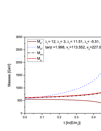
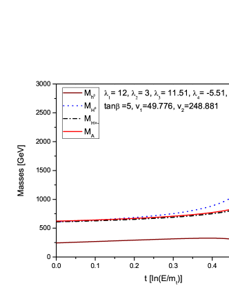
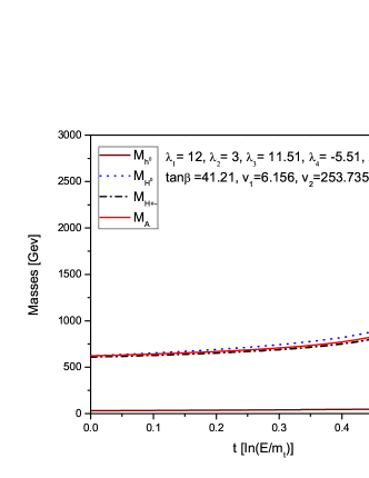
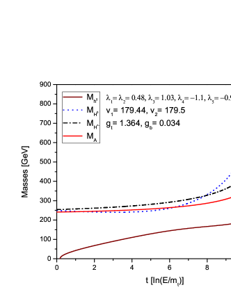
In general, according to Eqs. (29)-(31) the mass dependence on $v_{1},v_{2},\,\,$or$\,\,\,v=\sqrt{v_{1}^{2}+v_{2}^{2}},$ can be reformulated in terms of $v$ and $v_{2}.$ Therefore, with known $v$ one can plot those masses in terms of $v_{2\text{ }}$, and determine their dependence on $v_{2}$ or $\tan\beta$ ($\tan\beta=v_{2}/\sqrt{v^{2}-v_{2}^{2}}$), as in Fig. 1.

Figure 1: The $v_{2}$ dependence of the Higgs masses for various sets of quartic couplings.

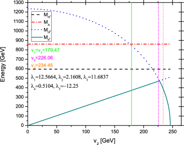
As the favoured Standard Model Higgs mass window is still open, and as the 2HDM Higgses are nonstandard, almost none of the masses range has yet been ruled out, one can explore several hypothetical situations and analize the consequences of some published values for $M_{H^{\pm}}$.

We will now proceed to numerically evaluate the Higgs masses under different conditions for the quartic parameters at the energy scale $E=M_{t}$, where $M_{t}$ is the mass of the quark top. First we will reproduce the $M_{H^{\pm}}$ value given in Stal , considering several sets of $\lambda$’s. We choose $\lambda_{4}=-5.52,$ and $\lambda_{5}=-6.0$ from many combinatios that give $M_{H^{\pm}}=609.1,M_{A^{0}}=621.7$. As we shall see, in the extreme case, with one of the symmetries considered in Maniatis in which $\lambda_{1}=\lambda_{2}=\lambda$, and $\tan\beta=1$, or $\tan\beta=5$ all the Higgs masses acquire constant values and $M_{h^{0}}=0$. With the previous $\lambda_{4}$, $\lambda_{5}$, we obtain for $H^{0}$ values which are not ruled out experimentaly (for the SM Higgs) according to D0 , in the following way: ($\lambda=0.485$, $\lambda_{3}=10.55$, $\lambda_{T}=-0.97$, $M_{H^{0}}=250$), ($\lambda=0.653$, $\lambda_{3}=10.21$, $\lambda_{T}=-1.30$, $M_{H^{0}}=290$) and ($\lambda=1.94$, $\lambda_{3}=7.64$, $\lambda_{T}=-3.88$, $M_{H^{0}}=600$).

Though the masses do not depend on $\tan\beta$ at this energy scale, we will explore, in the next section, their behavior and dependence on it at higher energies scales.

Let us now classify the several cases, we will consider , in terms of the different stability condiions for the $\lambda_{i}$ s

A.- Extreme case in which both equalities are satisfied

$$\lambda_{T}=-2\sqrt{\lambda_{1}\lambda_{2}},\,\,\,\,\,\,\,\cup\,\,\,\,\,\,\,\,\lambda_{1}/\lambda_{2}=\left(\tan\beta\right)^{4}$$ (87)

B1.- Semi-extreme case:

$$\lambda_{T}=-2\sqrt{\lambda_{1}\lambda_{2}},\,\,\,\,\,\,\lambda_{1}/\lambda_{2}\neq\left(\tan\beta\right)^{4}$$ (88)

B2.- Semi-extreme case:

$$\lambda_{T}\neq-2\sqrt{\lambda_{1}\lambda_{2}},\,\,\,\,\,\,\lambda_{1}/\lambda_{2}=\left(\tan\beta\right)^{4}$$ (89)

C.- Lagrange inequality condition

$$\lambda_{T}\geq-2\sqrt{\lambda_{1}\lambda_{2}}$$ (90)

D.- Yukawa - Universality condition

$$\tan\beta=M_{t}/M_{b},\,\,\,\,\,\,\,\,\,\,\,\,\,\,\,\,g_{t}=g_{b}$$ (91)

The former cases will be combined with two additional conditions for the quartic couplings:

Case 1 : $\lambda_{1}=\lambda_{2},$ and Case 2: $\lambda_{1}\neq\lambda_{2}.$
In case 1A , 2A and 1B, all the masses have a constant value in the inerval $0\leq v_{2}\leq v$ due to their only dependence on $v,$ but in spite of the an explicit independence of the masses on $v_{2}$ , $\tan\beta$ plays an important role on the energy scale dependence of the masses, as we shall see in the numerical solutions of the Renormalization Group Equations.which is fixed. In case 2B, M${}_{H^{0}}$ depends explicitly on $v_{2}$ and therefore on $\tan\beta.$

To compare with the masses $M_{H^{\pm}}=609,$ $M_{A}=621.7$ given in Ref.Stal , we consider three kinds of compositions of the $\lambda_{i}\,\,\,i=1,...,5$ parameters as in a), b) and c), which produce seven cases. The properties of these cases are to be analized in the following section.
a.-When $\left(\begin{array}[]{ccccc}\lambda_{1}&\lambda_{2}&\lambda_{3}&\lambda_{4}&\lambda_{5}\\ 0.485&0.485&10.55&-5.52&-6.0\end{array}\right)$ , which means that $\lambda_{T}=-2\sqrt{\lambda_{1}\lambda_{2}}=-0.97$ and $\left(\lambda_{1}/\lambda_{2}\right)^{1/4}=1.0,$ we obtain

$$\begin{array}[]{c}\text{Case}\\ 1A\\ 1D\end{array}\begin{array}[]{ccc}\tan\beta&M_{h^{0}}&M_{H^{0}}\\ 1.0&0&250\\ 41.2&0&250\end{array}\begin{array}[]{c}v_{2}\\ 179.47\\ 253.7\end{array}$$

b.- When $\left(\begin{array}[]{ccccc}\lambda_{1}&\lambda_{2}&\lambda_{3}&\lambda_{4}&\lambda_{5}\\ 6.0&1/6&9.51&-5.51&-6.0\end{array}\right)$, i.e., $\lambda_{T}=-2\sqrt{\lambda_{1}\lambda_{2}}=-2.0$ and $\left(\lambda_{1}/\lambda_{2}\right)^{1/4}=2.45,$ we obtain

$$\begin{array}[]{c}\text{Case}\\ 2A\end{array}\begin{array}[]{ccc}\tan\beta&M_{h^{0}}&M_{H^{0}}\\ 2.45&0&358.9\end{array}\begin{array}[]{c}v_{2}\\ 234.9\end{array}$$

c.- When $\left(\begin{array}[]{ccccc}\lambda_{1}&\lambda_{2}&\lambda_{3}&\lambda_{4}&\lambda_{5}\\ 12.0&3.0&11.5&-5.5&-6.0\end{array}\right)$ with $\lambda_{T}=0.0,-2\sqrt{\lambda_{1}\lambda_{2}}=-12.0$ and $\left(\lambda_{1}/\lambda_{2}\right)^{1/4}=1.4,$ we explore different $\tan\beta$ cases

$$\begin{array}[]{c}\text{Case}\\ 2B2\\ 2C\\ 2C\\ 2D\end{array}\begin{array}[]{ccc}\tan\beta&M_{h^{0}}&M_{H^{0}}\\ 1.4&507.6&717.9\\ 2.0&556.0&556.0\\ 5.0&243.9&609.6\\ 41.2&30.2&621.5\end{array}\begin{array}[]{c}v_{2}\\ 207.2\\ 227.0\\ 248.9\\ 253.7\end{array}$$

d.- Considering now smaller values for $\{M_{H^{\pm}},M_{A}\}=\{253.8,240.8\}$, with interesting properties for the energy range of validity of the 2HDM, with $\lambda_{T}=-2\sqrt{\lambda_{1}\lambda_{2}}=-0.97$ and $\left(\lambda_{1}/\lambda_{2}\right)^{1/4}=1.0$, for $\left(\begin{array}[]{ccccc}\lambda_{1}&\lambda_{2}&\lambda_{3}&\lambda_{4}&\lambda_{5}\\ 0.48&0.48&1.03&-1.1&-0.9\end{array}\right)$

$$\begin{array}[]{c}\text{Case}\\ 1A\\ 1D\end{array}\begin{array}[]{ccc}\tan\beta&M_{h^{0}}&M_{H^{0}}\\ 1.0&0&250\\ 41.2&0&250\end{array}\begin{array}[]{c}v_{2}\\ 179.5\\ 253.7\end{array}$$

e.- Finally, for even lower masses $\{M_{H^{\pm}},M_{A}\}=\{170.3,160.5\},$ which arise from $\left(\begin{array}[]{ccccc}\lambda_{1}&\lambda_{2}&\lambda_{3}&\lambda_{4}&\lambda_{5}\\ 0.125&0.125&0.65&-0.5&-0.4\end{array}\right)$, where $\lambda_{T}=-2\sqrt{\lambda_{1}\lambda_{2}}=-0.25$ and $\left(\lambda_{1}/\lambda_{2}\right)^{1/4}=1.0,$ we obtain

$$\begin{array}[]{c}\text{Case}\\ 1D,1B1\end{array}\begin{array}[]{ccc}\tan\beta&M_{h^{0}}&M_{H^{0}}\\ 41.2&0&127\end{array}\begin{array}[]{c}v_{2}\\ 253.7\end{array}$$

VI Triviality constrains.

Renormalization group equations

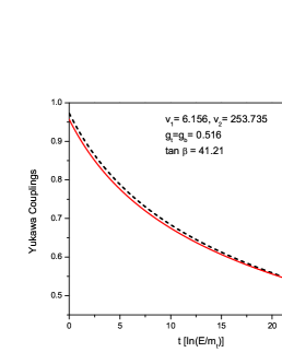
In this section we explore the asymptotic behavior of the parameters in the model, and their relations, through the Renormalization Group Equations (RGE) Inoue . The RGE are a powerful tool to determine by the triviality principle, the energy bounds of the parameters and the validity of the model. In order to proceed in this way, to numerically evaluate the energy dependence of the $\lambda_{i}$ quartic couplings, it is necessary to consider the RGE of all the parameters, i.e., the gauge group couplings $g_{1}$, $g_{2}$, $g_{3}$ of the symmetry groups $U(1),SU(2),SU(3)$, the vacuum expectation values $v_{1}$, $v_{2}$, and the Yukawa couplings of the top and the down quark sectors $g_{t}$ and $g_{d}$ respectively Refs. Arason .

The RGE determine the dependence of the coupling constants and other parameters of the Lagrangian on $t$, defined as $t=\ln\left(E/m_{t}\right)$, where $E$ is the renormalization point energy. The RGE for the gauge couplings $g_{1}$, $g_{2}$, $g_{3}$ are:

$$\frac{dg_{k}}{dt}=\frac{1}{(4\pi)^{2}}b_{k}g_{k}^{3}\quad(i=1,2,3),$$ (92)

The RGE for the Yukawa couplings of the top and bottom quarks $g_{t},g_{b}$ are

$$\frac{dg_{t}}{dt}=\frac{1}{(4\pi)^{2}}\left(\frac{9}{2}g_{t}^{2}+\frac{1}{2}g_{b}^{2}-(\frac{17}{20}g_{1}^{2}+\frac{9}{4}g_{2}^{2}+8g_{3}^{2})\right)g_{t},$$ (93)

$$\frac{dg_{b}}{dt}=\frac{1}{(4\pi)^{2}}\left(\frac{9}{2}g_{b}^{2}+\frac{1}{2}g_{t}^{2}-(\frac{1}{4}g_{1}^{2}+\frac{9}{4}g_{2}^{2}+8g_{3}^{2})\right)g_{b}$$ (94)

and for the vacuum expectation values $v_{1}$ and $v_{2}$

$$\frac{d}{dt}v_{1}=\frac{1}{(4\pi)^{2}}\left[-3g_{t}^{2}+(\left(9/20\right)g_{1}^{2}+\left(9/4\right)g_{2}^{2})\right]v_{1},$$ (95)

$$\frac{d}{dt}v_{2}=\frac{1}{(4\pi)^{2}}\left[-3g_{b}^{2}+(\left(9/20\right)g_{1}^{2}+\left(9/4\right)g_{2}^{2})\right]v_{2}$$ (96)

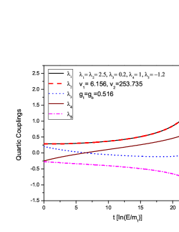
In the equations for the quartic couplings we include the quark Yukawa contributions of both sectors.

$$\frac{d\lambda_{1}}{dt}= \frac{1}{16\pi^{2}}\left\{24\left(\lambda_{1}\right)^{2}-3\lambda_{1}\left[3g^{2}+\left(g^{\prime}\right)^{2}-4g_{t}^{2}\right]+2\left(\lambda_{3}\right)^{2}+\left(\lambda_{4}\right)^{2}+\left(\lambda_{5}\right)^{2}\right.+\left.2\lambda_{3}\lambda_{4}+\frac{3}{8}\left(g^{2}+\left(g^{\prime}\right)^{2}\right)^{2}+\frac{3}{4}g^{4}-6g_{t}^{4}\right\},$$

$$\frac{d\lambda_{2}}{dt}= \frac{1}{16\pi^{2}}\left\{24\left(\lambda_{2}\right)^{2}-3\lambda_{2}\left[3g^{2}+\left(g^{\prime}\right)^{2}-4g_{b}^{2}\right]+2\left(\lambda_{3}\right)^{2}+\left(\lambda_{4}\right)^{2}+\left(\lambda_{5}\right)^{2}\right.+\left.2\lambda_{3}\lambda_{4}+\frac{3}{8}\left[\left(g^{\prime}\right)^{2}+g^{2}\right]^{2}+\frac{3}{4}g^{4}-6g_{b}^{4}\right\},$$

$$\frac{d\lambda_{3}}{dt}= \frac{1}{16\pi^{2}}\left\{4\left(\lambda_{3}\right)^{2}+4\left(3\lambda_{3}+\lambda_{4}\right)\left(\lambda_{1}+\lambda_{2}\right)-3\lambda_{3}\left[3g^{2}+\left(g^{\prime}\right)^{2}-2\left(g_{t}^{2}+g_{b}^{2}\right)\right]\right.$$ (97)

$$+\left.2\left(\lambda_{4}\right)^{2}+2\left(\lambda_{5}\right)^{2}+\frac{3}{4}\left[g^{2}-\left(g^{\prime}\right)^{2}\right]^{2}+\frac{3}{2}g^{4}-12g_{t}^{2}g_{b}^{2}\right\},$$

$$\frac{d\lambda_{4}}{dt}= \frac{1}{16\pi^{2}}\left\{4\left(\lambda_{4}\right)^{2}+4\lambda_{4}\left(\lambda_{1}+\lambda_{2}+2\lambda_{3}\right)-3\lambda_{4}\left[3g^{2}+\left(g^{\prime}\right)^{2}-2\left(g_{t}^{2}+g_{b}^{2}\right)\right]\right.+\left.8\left(\lambda_{5}\right)^{2}+3g^{2}\left(g^{\prime}\right)^{2}+12g_{t}^{2}g_{b}^{2}\right\},$$

$$\frac{d\lambda_{5}}{dt}= \frac{1}{16\pi^{2}}\lambda_{5}\left\{4\left(\lambda_{1}+\lambda_{2}+2\lambda_{3}+3\lambda_{4}\right)-3\left[3g^{2}+\left(g^{\prime}\right)^{2}-2\left(g_{t}^{2}+g_{b}^{2}\right)\right]\right\}.$$

The former equations are the coupled, non linear, ordinary differential equations whose solution provides the information about the renormalization point energy dependence of the masses of the five Higgs particles of the 2HDM. To numerically solve the RGE, the initial or final conditions for the parameters have to be previously chosen. In order to do so we use Ref. PDG . The range of values, we take, for the energy and the variable $t$ are $\left(E_{0}=M_{t},E_{u}\right)=\left(173.2,1.234\cdot 10^{13}\right)$, $\left(t_{0}=0,t_{u}=25\right)$ respectively, where $M_{t}$ stands for the mass of the quark top and $E_{u}$ corresponds to the electroweak unification energy where $g_{1}(E_{t})=g_{2}(E_{t})$. The gauge couplings $\left(g_{1},g_{2,}g_{3}\right)_{E=M_{t}}\simeq\left(0.4627,0.6466,1.2367,\right)$ are obtained using the following relations

$$\alpha_{e}(M_{t}) =g_{e}^{2}/4\pi=1/\left(127.9\right),\quad g_{1}(M_{t})=\sqrt{5/3}g_{e}/\cos\theta_{W}\,\quad$$

$$g_{2}(M_{t}) =g_{e}/\sin\theta_{W},\quad g_{3}(M_{t})=\sqrt{4\pi\alpha_{s}(M_{t})}$$

where $\theta_{W}$ is the Weinberg angle and $\sin^{2}\theta_{W}(M_{t})=0.235$ and $\alpha_{s}=0.1217$. The vev standard value that arises from

$$v=2M_{z}/\sqrt{g_{2}^{2}+g_{e}^{2}}$$

is $v(M_{t})=253.81$ GeV at $M_{z}=91.19$ GeV.
In order to specify more rigorously the energy limits for the quartic couplings, we have numerically solved the RGE for the gauge group couplings $g_{1}$, $g_{2}$, $g_{3}$, (Fig. 2), the vacuum expectation values $v_{1}$, $v_{2}$, and the top and the down quark Yukawa couplings $g_{t}$ and $g_{d}$, under the following assumptions:

• The heaviest quark masses are related with the vevs $v_{1}$ and $v_{2}$ and the Yukawa couplings $g^{(u)}$ and $g^{(d)}$

  $$M_{t}=\frac{v_{2}}{\sqrt{2}}g_{t},\quad\tan\beta=\frac{v_{2}}{v_{1}},\quad M_{b}=\frac{v_{1}}{\sqrt{2}}g_{b}.$$ (98)

• The gauge bosons masses are related with the gauge couplings $g^{\prime}$ and $g$

  $$M_{W}=\frac{1}{2}vg,\quad M_{Z}=\frac{M_{W}}{\cos\theta_{W}}=\frac{1}{2}v\sqrt{g^{2}+\left(g^{\prime}\right)^{2}},$$ (99)

  where $\theta_{W}$ is the Weinberg angle and $e$ the electron charge

  $$e=g\sin\theta_{W}=g^{\prime}\cos\theta_{W}.$$ (100)

• Unification of the Yukawa couplings at $E=M_{t}$ or at $E_{u}$, i.e., $g_{b}=g_{t}$, and $\tan\beta=M_{t}/M_{b}$.

Figure 2: The energy dependence of the gauge couplings in the 2HDM.

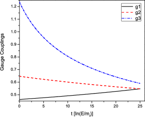
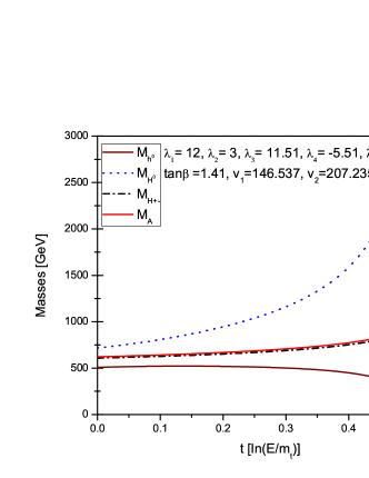
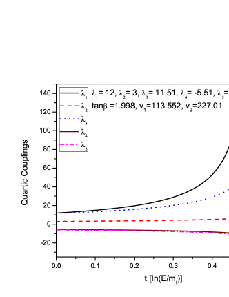
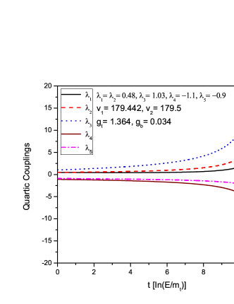
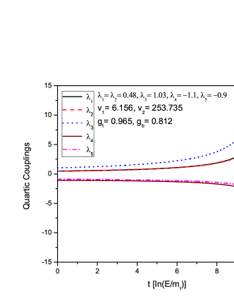
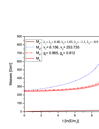
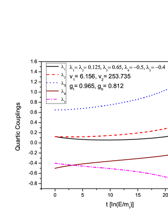
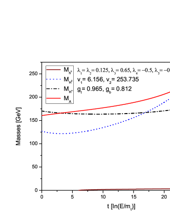
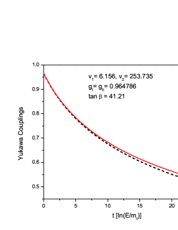
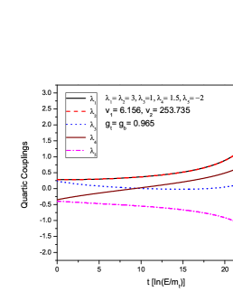
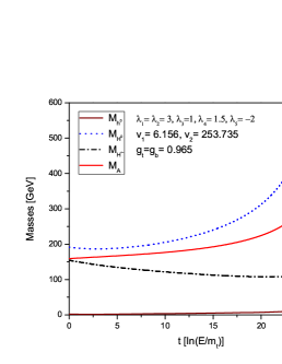
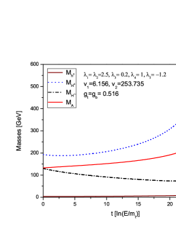
It is interesting to explore now, the energy bounds of the 2DHM, through the running of the quartic couplings which determine the mass values of the Higgses. In the case (c) considered in the previous section, when $M_{H^{\pm}}=609,$ $M_{A}=621.7$, the range of validity of the model is very short $M_{t}<E<292$ i.e., $0<t<0.52$ as can be seen in Figs. 3–6. There is an intermediate class of the models depicted at Figs. 7, 8, which have an intermadite range of validity $0<t\lesssim 11$. So we will rather focus our atention on the cases where we can explore the universality of the Yukawa couplings and its unification, to study the mass-hierarchy problem. In this case, as can be seen in Figs. 9–11, the 2HDM is valid in the whole range of energies, this means $M_{t}<E<E_{u}$ where $E_{u}$ is the electroweak unification energy. In Fig. 9 we observe very slow dependence of the quaric couplings and the Higgs masses on the renormalization point energy. This model is characterized by rather small values of the quartic Yukawa couplings and the value of $\tan\beta$ such that it permits the unification of the Yukawa couplings of the up and down quarks $g_{t}=g_{b}$. In Figs. 10, 11 we show the evolution of the Yukawa couplings, quartic couplings and the Higgs masses for the case when the Yukawa couplings are unified. In Fig. 10 we assume that they are unified at low energy and in Fig. 11 they are unified at high energy. The evolution of the quartic couplings and Higgs masses are similar in both cases.

Figure 3: The energy dependence of the quartic couplings and Higgs masses, case 2B2, with $\tan\beta=1.41$.

Figure 4: The energy dependence of the quartic couplings and the Higgs masses, case 2C with $\tan\beta=2.0$.

Figure 5: The energy dependence of the quartic couplings and the Higgs masses, case 2C with $\tan\beta=5.0$.

Figure 6: The energy dependence of the quartic couplings and the Higgs masses, case 2D with $\tan\beta=41.2$.

Figure 7: The energy dependence of the quartic couplings and the Higgs masses, case 1A with $\tan\beta=1$ (2D) case.

Figure 8: The energy dependence of the quartic couplings and the Higgs masses, case 1D with $\tan\beta=41.2$ (2D) case.

Figure 9: The energy dependence of the quartic couplings and the Higgs masses, case 1B1 with $\tan\beta=41.2$.

Figure 10: The energy dependence of the Yukawa couplings, quartic couplings and the Higgs masses in the $\tan\beta=41.2$ (1D) case with Yukawa couplings $g_{t}=g_{b}$ at low energy.

Figure 11: The energy dependence of the Yukawa couplings. quartic couplings and the Higgs masses in the $\tan\beta=41.2$ (1D) case with equal Yukawa couplings $g_{t}=g_{b}$ at high energy.

VII Results and conclusions

With the aim to explore the Higgs mass content of the 2HDM extension of the standard model, among the different forms of the Lagrangian describing the same physical reality, we have chosen a specific one, in which the vacuum expectation values of both Higgs fields are real, and for simplicity also preserving the CP symmetry. We have deduced, in this model, the analytical expressions for the masses of the five predicted physical Higgs particles, and expressed the Higgs potential in terms of those masses, using Eqs. (30) and (31). We have also obtained, through the mass formulas, a set of constraints to be satisfied by the scalar parameters that determine the couplings and self-couplings of the Higgs fields introduced in the potential Eq. (3), and through the vacuum stability principle plus the Lagrange Multipliers method, and obtained additional conditions to be satisfied by those couplings.

$$\lambda_{1}>0,\;\lambda_{2}>0,\quad 4\lambda_{1}\lambda_{2}>\left(\lambda_{3}+\lambda_{4}+\lambda_{5}\right)^{2},\quad\left(\lambda_{4}+\lambda_{5}\right)<0,\quad\lambda_{5}<0,\quad\lambda_{4}<\left|\lambda_{5}\right|,$$ (101)

and

$$\lambda_{1}+\lambda_{2}>\lambda_{3}+\lambda_{4}+\lambda_{5},\quad\lambda_{3}+\lambda_{4}+\lambda_{5}+2\sqrt{\lambda_{1}\lambda_{2}}>0,\quad\lambda_{3}+2\sqrt{\lambda_{1}\lambda_{2}}>0,\quad\ 4\left(\lambda_{1}\lambda_{2}\right)\neq\lambda_{3}^{2}.$$ (102)

We have also looked upon extreme and semiextreme conditions on the Higgs potential and gave a clasification of the different cases we analized under the RGE.

As many authors base their calulations in symmetry conditions, such as $\lambda_{1}=\lambda_{2}$ and others in a phenomenologycal study of special events, it is important to analize the consequences of such assumptions and we tried at least partially address this problem.

There is a batch of data to be analysed right now in search of some of the favored mass region, and all of it should be examined in the near future. The results of this paper may shed some light on physics of the Higgs sector depending on the properties of the Higgs particle.

We have considered here, symmetries in the $\lambda_{i}$ parameters, universality of the Yukawa couplings at low energy $E_{0}$ ($M_{t}$ scale) or high energy $E_{u}\,$(weak-unification scale), hierarchy of the quark masses and the energy range of validity of the model. The other symmetry considered here is the unification of the Yukawa couplings. It seems this symmetry makes the Higgs sector very stable as can be seen in Fig. 9.

In summary, the results in this paper may be a basis for further investigation in relation to the behavior and energy dependent characteristics of the Higgs particles.

We finish by allegorically saying, that our paper still contains a “blank page”, which can only be filled after the discovery of Higgs bosons.

References

- (1) S. Glashow, Nucl. Phys. 22 (1961) 579; S. Weinberg, Phys. Rev. Lett. 19 (1967) 1264; A. Salam, in Elementary Particle Theory (Nobel Symposium No. 8). Edited by N. Svarthholm, (Almquist and Wiksell. Stockholm, 1968).
- (2) K. Nakamura et al, Journal of Physics G 37, 075021 (2010)
- (3) S. Kraml, (164 additional authors not shown) arXiv:hep-ph/0608079 CERN-CPNSH Workshop, May 2004 - Dec. 2005. Ed. by Sabine Kraml, et. al. (GENEVA 2006).
- (4) P. W. Higgs, Phys. Lett. 12, 132 (1964).
- Note (1) \BibitemOpenThe importance of such analysis can be seen for example in the Higgs search scenarios, e.g., David López-Val and Joan Solà, Phys. Rev. D 81, (2010), Joan Solà, David López-Val, arXiv:1107.1305 [hep-ph].\BibitemShutStop
- Note (2) \BibitemOpenSee for example Apostolos Pilaftsis and Carlos E.M. Wagner, Nucl. Phys. 553, 3 (1999).\BibitemShutStop
- Note (3) \BibitemOpenThere are also other scenarios for the quark mass generation in the 2DHM but we will not be considering them here.\BibitemShutStop
- (8) K. Inoue, A. Kakuto and Y. Nakano, Prog. Theor. Phys. 63, 234 (1980).
- (9) J.F. Gunion, H.E. Haber, G.L. Kane and S. Dawson, The Higgs hunter´s guide (Addison-Wesley, Reading, MA, 1990).
- (10) D. Kominis and R. Sekhar, Phys. Lett. B304, 152 (1993).
- (11) S. L. Glashow, J. Iliopoulos and L. Maiani, Phys. Rev. D 2 1285 (1977) 1285.
- (12) P. Kielanowski, S.R. Juárez W. and H.G. Solís-R., Phys. Rev. D 72, 96003 (2005).
- Note (4) \BibitemOpenTo make the discussion more transparent we introduced a different parametrization of the Higgs potential in this section.\BibitemShutStop
- Note (5) \BibitemOpenThe vacuum stability constrains for the Higgs potential do not depend on the quadratic part of the Higgs potential and for this reason we do not include it in our discussion.\BibitemShutStop
- (15) F. Mahmoudi and O. Stål, Phys. Rev. D 81, 035015 (2010); D. Eriksson, F. Mahmoudi, J. Rathsman, O. Stål, Constraints on the Two-Higgs-Doublet Model Uppsala University. SUSY09. Northeastern University, Boston. 5-10 June 2009. http://www.isv.uu.se/thep/talks/os/090608-2hdm.pdf.
- (16) M. Maniatis, A. von Manteuffel, O. Natchmann, F. Nagel, Eur. Phys. J. C 48, 805-823 (2006).
- (17) CMS-PAS-HIG-11-023, ATLAS-CONF-2011-157.
- (18) C.R. Das, M.K. Parida, Eur. Phys. J. C 20, 121 (2001); H. Arason, D. J. Casta o, E. J. Piard, and P. Ramond Phys. Rev. D 47, 232 (1993).