The role of boundaries in the MagnetoRotational Instability

Abstract

In this paper, we investigate numerically the flow of an electrically conducting fluid in a cylindrical Taylor-Couette flow when an axial magnetic field is applied. To minimize Ekman recirculation due to vertical no-slip boundaries, two independently rotating rings are used at the vertical endcaps. This configuration reproduces setup used in laboratory experiments aiming to observe the MagnetoRotational Instability (MRI). Our 3D global simulations show that the nature of the bifurcation, the non-linear saturation, and the structure of axisymmetric MRI modes are significantly affected by the presence of boundaries. In addition, large scale non-axisymmetric modes are obtained when the applied field is sufficiently strong. We show that these modes are related to Kelvin-Helmoltz destabilization of a free Shercliff shear layer created by the combined action of the applied field and the rotating rings at the endcaps. Finally, we compare our numerical simulations to recent experimental results obtained in the Princeton MRI experiment.

I Introduction

The magnetorotational instability has provided a simple explanation of the longstanding problem of rapid angular momentum transport in accretion disks around stars and black holes BalbusHawley91. Balbus and Hawley, rediscovering an instability first studied by Velikhov Velikhov59 and Chandrasekhar Chandra60 , have shown that keplerian flows of accretion discs, for which the Rayleigh criterion predicts axisymmetric hydrodynamical stability, can be destabilized in the presence of a magnetic field. More precisely, the MRI is a linear instability occurring when a weak magnetic field is applied to a rotating electrically conducting fluid for which the angular velocity decreases with the distance from the rotation axis, i.e. $\partial_{R}(\Omega^{2})<0$. Linear stability analysis indicates that the most unstable mode is axisymmetric and associated with a strong radial outflow of angular momentum. Non-linear evolution of the MRI is of primary importance, since saturation of the instability eventually yields a magnetohydrodynamical turbulent state, enhancing the angular momentum transport.

During the last decade, there has been a lot of effort to observe the MRI in a laboratory experiment. To this end, most groups use a magnetized Taylor-Couette flow, i.e. the viscous flow of an electrically conducting fluid confined between two differentially rotating concentric cylinders, in the presence of an externally imposed magnetic field. For infinitely long cylinders, the ideal laminar Couette solution is given by:

$$\Omega(r)=A_{1}+\frac{A_{2}}{r^{2}}$$ (1)

in which $A_{1}=(\Omega_{2}r_{2}^{2}-\Omega_{1}r_{1}^{2})/(r_{2}^{2}-r_{1}^{2})$ and $A_{2}=r_{1}^{2}r_{2}^{2}(\Omega_{1}-\Omega_{2})/(r_{2}^{2}-r_{1}^{2})$, $\Omega_{1}$ and $\Omega_{2}$ are respectively the angular velocity of inner and outer cylinder, and $r_{1}$, $r_{2}$ are the corresponding radii. The Rayleigh criterion predicts axisymmetric linear stability if $\Omega_{2}/\Omega_{1}\geq(r_{1}/r_{2})^{2}$, ensuring that the specific angular momentum increases outward. However, MRI may arise if $\Omega_{2}/\Omega_{1}<1$ and non-ideal MHD effects are small Ji01 .

Several experiments are currently working on MRI. The Princeton experiment has been designed to observe this instability in a Taylor-Couette flow of liquid Gallium, with an axial applied magnetic field Ji06 . So far, MRI has not been identified, but non-axisymmetric modes have been observed when a strong magnetic field is imposed Nornberg10 . The PROMISE experiment, in Dresden, is based on a similar set-up, except that the applied field possesses an azimuthal component. Axisymmetric traveling waves have been obtained, and identified as being Helical MRI, an inductionless instability different from but connected to the standard MRI Stefani06 . A few years ago, MRI was claimed to have been obtained in a spherical Couette flow of liquid sodium (hereafter “Maryland experiment”) Sisan04 . In this experiment, in which the outer sphere was at rest and a poloidal magnetic field was applied, non-axisymmetric oscillations of both velocity and magnetic fields were observed, together with an increase of the torque on the inner sphere. However, it has been shown recently that these oscillations were more likely related to instabilities of magnetic free shear layers in the flow Gissinger11 , Hollerbach09 .

Experimental observation of the MRI is considerably complicated by the presence of vertical boundaries. Indeed, no-slip boundary conditions at the vertical endcaps (for instance rigidly rotating with either the outer or the inner cylinder) induce an imbalance between the pressure gradient and the centrifugal force, and drive a meridional Ekman recirculation in addition to the azimuthal Couette flow. An inward boundary-layer flow near the endcaps is balanced by strong outward jet at the midplane. This Ekman recirculation has two important consequences for laboratory MRI: first, the meridional flow transports angular momentum outward, decreasing the free energy available to excite MRI. Moreover, the Ekman flow is a source of hydrodynamical fluctuations, beginning at Reynolds numbers $\gtrsim 400$ with oscillations of the radial jet Kageyama04 , which strongly complicates the identification of MRI modes.

In the Princeton MRI experiment, this problem has been circumvented by replacing the rigid endcaps at the top and the bottom by two rings that are driven independently, reducing the imbalance due to viscous stress. It has been shown that a quasi-keplerian flow profile $(r_{1}/r_{2})^{2}<\Omega_{2}/\Omega_{1}<1$ in a short Taylor-Couette cell can be kept effectively stable up to $Re\sim 10^{6}$ if appropriate ring speeds are used Ji06 . Similarly, the PROMISE group found that split rings (attached to the cylinders rather than independently driven) led to a significant reduction of the Ekman pumping and a much clearer identification of the HMRI Stefani09 .

In this article, we report three-dimensional numerical simulations inspired by these experimental configurations, especially the Princeton MRI experiment. In the first section, we present the equations and the numerical method used. In section II, we study how the structure and the saturation of the magnetorotational instability arising in Taylor-Couette flow is modified by the presence of vertical boundaries. In section III, we report new non-axisymmetric instabilities generated by a free shear layer in the flow when the applied field is sufficiently strong compared to the rotation. Finally, a comparison with results from the Princeton MRI experiment is presented.

II Equations

We consider the flow of an electrically conducting fluid between two co-rotating finite cylinders. $r_{1}$ is the radius of the inner cylinder, $r_{2}=3r_{1}$ is the radius of the outer cylinder, and $d=r_{2}-r_{1}$ is the gap between cylinders. $\Omega_{1}$ and $\Omega_{2}$ are respectively the angular speed of the inner and the outer cylinder. The height of the cylinders $H$ is fixed such that we have the aspect ratio $\Gamma=H/d=2$, as in the Princeton MRI experiment. A uniform background magnetic field $\boldsymbol{B}_{0}=B_{0}\boldsymbol{e}_{z}$ is imposed by external coils.

The governing equations for this problem are the Navier-Stokes equations coupled to the induction equation :

$$\rho\frac{\partial\boldsymbol{u}}{\partial t}+\rho\left(\boldsymbol{u}\cdot\boldsymbol{\nabla}\right)\boldsymbol{u}=-\boldsymbol{\nabla}P+\rho\nu\boldsymbol{\nabla}^{2}\boldsymbol{u}+\boldsymbol{j}\boldsymbol{\times}\boldsymbol{B}\ .$$ (2)

$$\frac{\partial\boldsymbol{B}}{\partial t}=\boldsymbol{\nabla}\boldsymbol{\times}\left(\boldsymbol{u}\boldsymbol{\times}\boldsymbol{B}\right)+\frac{1}{\mu_{0}\sigma}\boldsymbol{\nabla}^{2}\boldsymbol{B}\ .$$ (3)

where $\rho$ is the density, $\nu$ the kinematic viscosity, $\eta=1/(\sigma\mu_{0})$ is the magnetic diffusivity, $\boldsymbol{u}$ is the fluid velocity, $\boldsymbol{B}$ the magnetic field, and $\boldsymbol{j}=\mu_{0}^{-1}\boldsymbol{\nabla}\boldsymbol{\times}\boldsymbol{B}$ the electrical current density. The problem is characterized by three dimensionless numbers: the Reynolds number $Re=(\Omega_{1}r_{1}d)/\nu$, the magnetic Reynolds number $Rm=(\Omega_{1}r_{1}d)/\eta$ and the Lundquist number $S=B_{0}r_{1}/(\sqrt{\rho\mu_{0}}\eta)$. Alternatively, the applied field can be measured by the Hartmann number $M=B_{0}r_{1}/\sqrt{\rho\mu_{0}\eta\nu}$, or the Elsasser number $\Lambda=B_{0}^{2}/(\rho\mu_{0}\eta\Omega)$. It is also useful to define the magnetic Prandtl number $Pm=\nu/\eta$, which is simply the ratio between Reynolds numbers. At the top and bottom, the endcaps are divided at $r=(r_{1}+r_{2})/2$ between two independently concentric rotating rings. Rotation rates of inner and outer rings are given respectively by $\Omega_{3}$ and $\Omega_{4}$.

These equations are integrated with the HERACLES code Gonzales06 . Originally developed for radiative astrophysical compressible and ideal-MHD flows, HERACLES relies on a finite volume Godunov method. The code has been parallelized with the MPI library and implemented in Cartesian, cylindrical and spherical coordinates. We have modified this code to include fluid viscosity, magnetic resistivity, and suitable boundary conditions for velocity and magnetic fields. Note that HERACLES is a compressible code, whereas laboratory experiments generally involve almost incompressible liquid metals. In fact, incompressibility corresponds to an idealization in the limit of infinitely small Mach number ($Ma$). In the simulations reported here, we used an isothermal equation of state with a sound speed such that $Ma<0.1$, following the approach of Liu06 ,Liu08 . Typical resolutions used in the simulations reported in this article are $(N_{r},N_{\phi},N_{Z})=[200,64,400]$. For some runs, we have checked that doubling this resolution does not affect results.

Except where indicated, the Reynolds number has been fixed at $Re=4000$, whereas $Rm$ and $S$ vary widely. On the cylinder sidewalls, at $r=r_{1}$ and $r=r_{2}$, we impose perfectly electrically conducting boundaries :

$$B_{r}=0\ ,\hskip 15.0pt{\partial B_{z}}/{\partial r}=0\ ,\hskip 15.0pt{\partial B_{\phi}}/{\partial r}=0$$ (4)

At the vertical endcaps, we use the so-called pseudo-vacuum boundary conditions, namely the magnetic field is forced to be normal to the boundary:

$$B_{r}=0\ ,\hskip 15.0ptB_{\phi}=0\ ,\hskip 15.0pt{\partial B_{z}}/{\partial z}=0$$ (5)

With these conditions, no magnetic torques are exerted through the boundaries. For the velocity field, no-slip boundary conditions are used for radial and axial components. The angular velocity matches the rotation rates of cylinders and rotating rings at radial and axial boundaries.

III Magneto-rotational instability in finite geometry

III.1 Purely hydrodynamical simulations

Accretion discs result from the balance between gravitation and centrifugal force, leading to an angular velocity profile such that $\Omega\sim r^{-3/2}$. Since the Rayleigh criterion states that any inviscid flow with rotation profile $\Omega\sim r^{\delta}$ is linearly stable to the centrifugal instability if $\delta>-2$, accretion discs are expected to be hydrodynamically linearly stable. Although Keplerian profiles can not be reproduced in the laboratory, it is possible to drive a Taylor-Couette flow in the so-called quasi-keplerian regime, i.e. with an angular momentum which increases outward to satisfy Rayleigh stability criterion, but which is MRI unstable (the angular velocity decreases outward). Except where indicated, all simulations reported here use the following rotation rates for the cylinders and rings:

$$\Omega_{1}=1.\ ,\hskip 10.0pt\Omega_{2}=0.13\ ,\hskip 10.0pt\Omega_{3}=0.45\ ,\hskip 10.0pt\Omega_{4}=0.16\$$ (6)

where rotation rates have been normalized by $\Omega_{1}$. The ratio $\Omega_{2}/\Omega_{1}$ ensures a quasi-keplerian regime, whereas $\Omega_{3}$ and $\Omega_{4}$ have been carefully chosen to strongly reduce Ekman recirculation and therefore reinforce the hydrodynamical stability of the flow Liu08 .

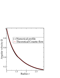
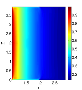
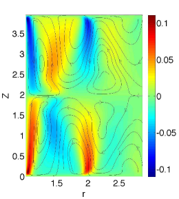
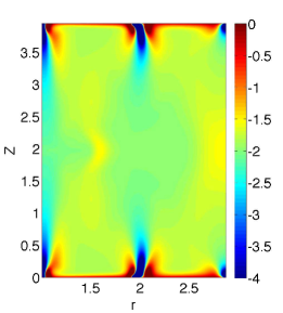
Figure 1: Purely hydrodynamical axisymmetric Taylor-Couette flow, obtained for $Re=4000$, $Rm=15$, $S=0$ and rotations rates given by eq.(6). Top, left: profile of $\Omega$ at $z=h/4$. Top, right: angular velocity $\Omega$ in $(r,z)$ plane. Bottom, left: $U_{z}$ in the $(r,z)$ plane (streamlines indicate meridional flow). Bottom, right: Shear $q$ (see eq. (7) ) in the $(r,z)$ plane. The use of rings at endcaps allows the flow to be very close to theoretical circular Couette flow. There is a weak poloidal recirculation, with $8$ unsteady cells. Except close to the boundaries, the shear is relatively uniform.

Figure 1 shows the flow obtained with the aforementioned standard parameters but without magnetic field, and for an axisymmetric simulation. Note that the radial profile of angular velocity matches almost perfectly the theoretical Couette solution (Fig. 1, top-left) that would be obtained with infinite or $z$-periodic cylinders. In fact, figure 1,top-right shows that the Couette profile prevails not only in the midplane, but in most of the domain. As expected, the use of rotating rings at the endcaps strongly reduces the Ekman flow, dividing the usual two big Ekman cells into eight smaller and less intense cells (Fig. 1,bottom-left). This structure is unsteady and the corresponding weak poloidal flow fluctuates as time evolves. The amplitudes of $u_{r}$ and $u_{z}$ are one order of magnitude smaller than for endcaps rotating with the outer cylinder.

To compare our numerical results to theoretical predictions, it is useful to define a local shear parameter $q$:

$$q=\frac{r}{\Omega(r)}\frac{\partial\Omega(r)}{\partial r}$$ (7)

For instance, in a keplerian flow $q$ would have the constant value $-3/2$. Figure 1,bottom-right shows $q$ in the $(r,z)$-plane for our system. In the bulk of the flow, $q$ is between $-1.5$ and $-2$ and matches the value corresponding to an ideal circular Couette flow. However, close to the endcaps, a very strong shear is generated where the rings meets, characterized by $q<-3.5$, reflecting Rayleigh-unstable flow. This corresponds to a cylindrical Stewartson free shear layer Stewartson66 at $r=(r_{1}+r_{2})/2$, created by the jump of the angular velocity between the two independently rotating rings. See Liu08b for a more detailed numerical study of this layer. Although one could expect a destabilization of this shear layer to large scale non-axisymmetric modes Hollerbach05 , this has not been observed in our simulations. Note that the layer does not extend very far from the endcaps, suggesting that it is disrupted by small-scale instabilities.

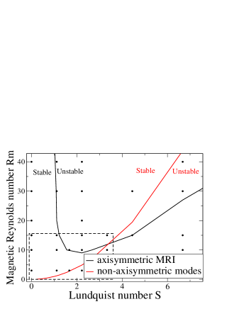
Figure 2: Stability boundaries in the plane of magnetic Reynolds number, $Rm$, versus Lundquist number, $S$. Black curve indicates the marginal stability curve of the MagnetoRotational Instability (MRI) obtained by interpolation from $2D$ simulations. Red curve is the marginal stability curve of non-axisymmetric modes generated by Kelvin-Helmoltz destabilization of the MHD detached shear layer, obtained from $3D$ simulations (black dots). Dashed square indicates the parameter space accessible to the Princeton experiment.

III.2 Imperfect bifurcation of the magnetorotational instability

Let us now consider the magnetized problem, meaning that a homogeneous axial magnetic field is now applied at the beginning of the simulation. As expected from global and local linear analyses, the flow is destabilized to MRI for sufficiently large $Rm$ and $S$. Figure 2 shows the marginal stability curve of the MRI (black curve) in the plane defined by these parameters. In the domain explored here, MRI modes are always axisymmetric. Linear stability analysis predicts non-axisymmetric MRI modes for $Rm>50$, which is larger than considered here. Note that the non-axisymmetric modes in Fig. 2 are not standard MRI but are related to the instability described in the next section. If the applied field is too strong, MRI modes are suppressed, and the flow is restabilized to a laminar state dominated by the azimuthal velocity. As a consequence, MRI modes are unstable only within the pocket-shaped interior of the black curve.

Figure 3 shows the structure of the MRI mode obtained in the saturated regime, for $Rm=15$ and $S=2.3$. Here, the structure of the MagnetoRotational Instability mainly consists of two large poloidal cells, as shown in the left panel. The corresponding radial magnetic field is shown on the right. At the endcaps, the fluid is strongly ejected and generates an outflowing narrow jet. The recirculation takes the form of a broad inflowing jet Liu08 . Consequently, we see that the MRI modes resemble the hydrodynamic Ekman circulation obtained when the endcaps corotate with the outer cylinder, except that the circulation is reversed. In fact, MRI modes are relatively similar to the classical Taylor vortices obtained in hydrodynamical Taylor-Couette flow.

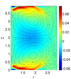
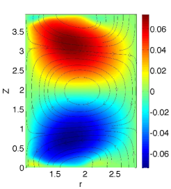
Figure 3: Structure of the MagnetoRotational Instability (MRI) mode when a magnetic field is applied in the $z$-direction, obtained for $Rm=15$ and $S=2.3$. Left: Radial velocity $U_{r}$ in the $(r,z)$ plane. Curves are streamlines of the poloidal flow. Right: radial magnetic field component $B_{r}$(normalized by the applied field $B_{Z}^{0}$) with magnetic field lines contained in the $(r,z)$ plane. For these boundary rotations [eq. (6)], MRI is characterized by a strong inflowing jet.

To follow the evolution of this large scale MRI mode, we compute the global quantity $A=\sqrt{V^{-1}\int_{V}{B_{r}^{2}dV}}$, where $V$ is the total volume between cylinders. Figure 4 shows the saturated value of $A$ as a function of the Lundquist number, for $Rm=15$. To understand how the MRI is generated in our finite geometry, it is useful to compare this bifurcation diagram to results obtained with periodic (or infinite) cylinders in the $z$ direction. In Figure 4, the black curve thus indicates results obtained with our no-slip rotating endcaps, whereas the red curve shows the diagram obtained when vertically periodic boundary conditions are used.

With periodic boundary conditions, the bifurcation of $A$ is characterized by a well defined critical Lundquist number $S_{c}$ above which MRI is observed ($S_{c}\sim 0.25$ for $Rm=15$). The magnetic field follows a classical square root law $A\sim\pm\sqrt{S-S_{c}}$ slightly above the MRI threshold $S_{c}$, and is zero below $S_{c}$. In this case, the solution is relatively similar to the one obtained with no-slip boundaries, except that the axial position of the outflowing jet is made arbitrary by the periodic boundaries, and the linear MRI modes are sinusoidal in the $z$ direction. In the linear regime, MRI modes correspond to the unstable branch appearing from the coalescence of two complex conjugate MagnetoCoriolis (MC) waves Nornberg10 . If these MC-waves are linearly stable (as in our simulations), the non-linear transition to MRI corresponds, at least close to the threshold $S_{c}$, to a classical supercritical pitchfork bifurcation:

$$\dot{A}=\mu A-A^{3}$$ (8)

where the dot denotes time derivative, and $\mu\propto S-S_{c}$ is a control parameter. Each of the two supercritical branches of solutions ($A=\pm\sqrt{\mu}$) is a transposition of the other corresponding to a phase-shift of one-half period, reflecting the arbitrary position of the MRI jet. For instance, the upper branch will correspond to an MRI mode with an outflow in the midplane, whereas the lower branch will represent MRI mode with inflow in the midplane. A schematic view of this supercritical bifurcation is shown in the lower panel of Fig. 4 by the red line.

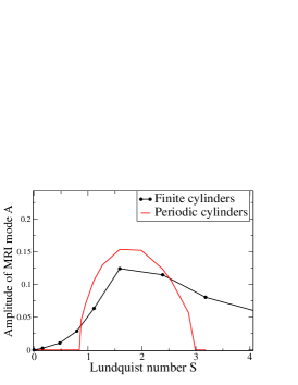
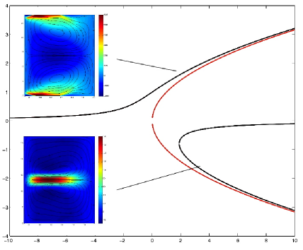
Figure 4: Top: Bifurcation diagram of the radial magnetic energy $A$ as a function of $S$ for $Rm=15$. Red curve correspond to periodic boundary conditions in $z$, whereas the black one corresponds to results obtained with no-slip rotating rings at the endcaps. In the latter case, the bifurcation is an imperfect supercritical pitchfork bifurcation due to the poloidal flow. Bottom: Schematic representation of perfect (red) and imperfect (black) pitchfork bifurcations of the MRI. Each branch corresponds to a different structure of the MRI mode: insets show MRI mode obtained from rotation rates given by eq.(6) (top-inset) or eq.(10) (bottom-inset).

However, no-slip vertical boundary conditions significantly change the nature of the bifurcation: with finite cylinders, we see in figure 4,top (black curve) that the evolution of $A$ is more gradual, and the definition of a critical onset $S_{c}$ is not well defined. In a finite geometry, the magnetorotational instability rather corresponds to an imperfect supercritical pitchfork bifurcation:

$$\dot{A}=\mu A-A^{3}+h$$ (9)

Here, $h$ is a symmetry-breaking parameter reflecting the absence of $z$-periodicity of the solutions, and forbidding the $A\rightarrow-A$ symmetry obtained in the case of periodic or infinite cylinders. Figure 4,bottom shows a schematic diagram of supercritical pitchfork bifurcations, in perfect and imperfect cases. Physically, this symmetry breaking means that for any value of the applied magnetic field, there is always a non-zero solution corresponding to the small poloidal recirculation created by the endcaps (see Figure 1,bottom-left). Therefore, with realistic boundaries, the magnetorotational instability continuously arises from this residual magnetized return flow, so that the axial position of the MRI outflowing jet is no longer arbitrary. This can be regarded as an analogue of the transition encountered in finite Taylor-Couette flow, in which Taylor vortices gradually emerges from the Ekman flow located at the endcaps Benjamin81 . Figure 4-top also shows that for strong applied field, the magnetic tension suppresses MRI modes. It is interesting to note that again, this restabilization is much more gradual in finite geometry than in the periodic case.

The modified nature of the bifurcation in the presence of realistic boundaries has important implications for experimental observations of the instability, because it strongly complicates the definition of an onset for the MRI. Since a recirculation is always generated by the boundaries, it will be difficult to distinguish an MRI mode from a simple magnetized meridional return flow, at least close to the instability threshold. If the generation of the magnetorotational instability in laboratory experiments corresponds to a strongly imperfect pitchfork bifurcation, as suggested by our numerical results, one can expect the following:

- First, the MRI will appear with the imperfect scaling obtained after integration of equation (9) instead of a classical square root law. On the one hand, this means that the transition to instability in bounded systems will not be as clear-cut as formerly expected, especially in experiments where only small $Rm$ can be obtained. On the other hand, the gradual transition to MRI means that some of the typical features of the instability can be observed below the expected onset of the MRI.

-Different structures for the MRI are obtained depending on the hydrodynamical configuration. This is directly related to the imperfect nature of the bifurcation: the residual flow due to the boundaries strongly affects the geometry of the unstable mode. For instance, the mode shown in Figure 3 has been obtained from the hydrodynamical state given by eq.(6) and shown in Figure 1. Without magnetic field, a weak outflow near the endcaps is produced, and the MRI mode generated in this case consists of poloidal vortices with the same outflowing jet near the endcaps. In other words, the hydrodynamical flow favors the upper branch of the pitchfork bifurcation, as in Figure 4-bottom. A different hydrodynamical configuration would lead to a different MRI mode. Consider for instance the following rotation rates:

$$\Omega_{1}=1.\ ,\hskip 10.0pt\Omega_{2}=\ \hskip 3.0pt\Omega_{3}=\ \hskip 3.0pt\Omega_{4}=0.13\$$ (10)

Here, the endcap rings are rigidly rotating with the outer cylinder. The unmagnetized flow is characterized by a strong inflow near endcaps, and the outflow is now localized in the midplane. In the presence of a magnetic field, MRI modes show a similar geometry, with a strong outflow in the midplane. This corresponds to change $h$ to $-h$ in the equation (9), thus selecting the lower branch mode $-A$ instead of $A$ (this MRI mode is shown in the lower inset of Figure 4).

-Finally, Figure 4-bottom illustrates that in the case of an imperfect bifurcation, one of the branches is replaced by a saddle-node bifurcation of two modes, one stable and the other unstable, predicting the possible co-existence of two MRI modes with different geometries. Note that the transition to this new mode would be strongly subcritical. This is the equivalent of the well known “anomalous modes” observed in hydrodynamical Taylor-Couette flows. Due to its subcritical nature, this mode has not been observed in our simulations, the lower inset in Figure 4-bottom corresponding to a simulation with rotation rates given by eq. (10), when the lower branch is continously connected to the Ekman flow.

III.3 Saturation of the MRI

In all the simulations reported here, most of the parameters have values comparable to those of laboratory experiments. For instance, in the Princeton experiment, the magnetic Reynolds number $Rm$ can be varied from $0$ to $15$, whereas the Lundquist number $S$ is between $0$ and $3$. The exception is the hydrodynamical Reynolds number, which can exceed $10^{6}$ in the experiments, whereas our simulations are limited by numerical resolution to $Re<2\times 10^{4}$. It is thus important to understand how our numerical results scale to a system with $Re\sim 10^{6}$. Figure 5 shows the evolution of the saturation of the MRI as a function of the Reynolds number.

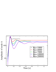
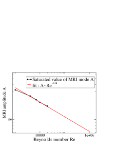
Figure 5: Effect of the hydrodynamical Reynolds number Re on the growth of MRI modes. The magnetic Reynolds number and the Lundquist number are kept fixed to $Rm=30$ and $S=4.5$. Top: Time evolution of the radial magnetic field density $A$ as a function of time, for different values of $Re$. Linear growth rates are independent of $Re$ but the saturation level strongly depends on $Re$. Bottom: evolution of the saturated value of $A$ as a function of $Re$. The saturation value of the MRI strongly decreases with $Re$. Red line indicates a fit corresponding to the scaling $A\sim Re^{-1/4}$

Figure 5-top shows the time evolution of the radial magnetic field density for different Reynolds numbers, ranging from $Re=10^{3}$ to $Re=2\times 10^{4}$. In the linear phase, all the growth rates are the same, illustrating the relevance of the linear inviscid theory and the weak role played by the Reynolds number. On the contrary, the saturation level depends on the Reynolds number: as $Re$ increases, the instability saturates to smaller values. It seems that the saturation of the MRI in our simulations scales like $A\sim Re^{-\beta}$, with $\beta=1/4$. This is a dramatic illustration of the challenges of observing MRI experimentally, where $Re$ must be several millions in order to achieve $Rm>1$ because of the properties of liquid metals. However, a naive extrapolation of our numerical results suggests that the magnetorotational instability in the Princeton experiment should saturate at a value only one order of magnitude smaller than in the simulations reported here, and should be measurable.

This scaling with $Re$ is directly related to the nature of the non-linear saturation mechanisms involved in Taylor-Couette flows. Indeed, it has been suggested by Knobloch et al Knobloch05 that in such Taylor-Couette devices, saturation mainly occurs by modification of the mean azimuthal profile: the shear in the flow is reduced, and is ultimately controlled by viscous coupling to the boundaries. Note that a simple dimensionless analysis shows that the exponent $\beta$ of our scaling corresponds to a balance between the Ekman pumping ($\sim Re^{-1/2}$) and the Maxwell stress tensor ($\sim B^{2}$), in agreement with this scenario. However, it is important to note that the saturation of the MRI is expected to be strongly different in discs, where shear is fixed and boundaries may be stress-free.

IV Non-axisymmetric instabilities

Let us now consider strongly magnetized situations. Figure 6 shows the same as Figure 1, but for an applied field such that $S=7$. In all the simulations reported here, the magnetic field is applied at the beginning of the simulation when the flow is at rest, letting the flow dynamically adapts as time evolves. At these large fields, we first note that the angular velocity profile is significantly different from the ideal Couette profile. In particular, the profile is steeper close to the inner cylinder and around $r=(r_{1}+r_{2})/2$. The distribution of the shear parameter $q$ (Fig. 6c) shows that the Stewartson shear layer (characterized by $q>-3.5$), confined to the endcaps in the purely hydrodynamical case, now penetrates deep inside the bulk of the flow Liu08b : the applied magnetic field, by uniformizing the flow in the $z$-direction, reinforces and extends the shear between rings. This leads to the generation of a new free shear layer, different from the Stewartson layer. In addition, note that the poloidal flow is strongly affected by the applied field. The eight poloidal cells generated in the non-magnetic case are reinforced, and aligned in the $z$-direction. A strong axial jet develops at $r=(r_{1}+r_{2})/2$, where the flow is ejected from the ring separation to the midplane.

A similar magnetized free shear layer has been extensively described in spherical geometry. The shear layer appears when a strong magnetic field is applied to a spherical Couette flow, the magnetic tension coupling fluid elements together along the direction of magnetic field lines. In the case of an axial magnetic field, this creates a particular surface $\Sigma$ located on the tangent cylinder, the cylindrical surface tangent to the inner sphere. Fluid inside $\Sigma$, coupled by the magnetic field only to the inner sphere, co-rotates with it, whereas fluid outside $\Sigma$ (coupled to both spheres) rotates at an intermediate velocity. The jump of velocity on the surface $\Sigma$ therefore results in a free shear layer, sometimes called Shercliff layer Shercliff53 . The thickness $\gamma$ of this MHD free shear layer is expected to vary like $\gamma\sim r/\sqrt{M}$, where $M$ is the Hartmann number. In our case, the Shercliff layer occurs on the cylindrical surface of radius $r=(r_{1}+r_{2})/2$, which separates regions of fluid coupled to the inner rings from fluid coupled to the outer rings.

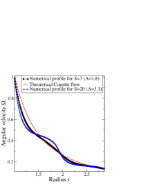
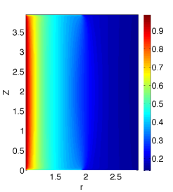
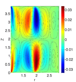
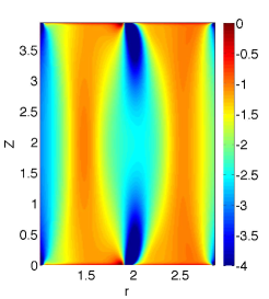
Figure 6: Taylor-Couette flow when a strong uniform magnetic field $B_{z}$ is applied in the axial direction $z$, obtained for $(\Omega_{1},\Omega_{3},\Omega_{4},\Omega_{2})=(400,180,65,53)$, $Rm=15$, $S=7$. Top-left: profile of $\Omega$ at $z=h/4$. Top-right: Angular velocity $\Omega$ in $(r,z)$ plane. We also show the profile obtained for $S=20$. Bottom-left: $U_{z}$ in the $(r,z)$ plane (streamlines indicate meridional flow. Bottom-right: Shear $q$ in the $(r,z)$ plane. The magnetic field tends to homogenize the flow in the $z$-direction. The jump of velocity between rings at endcaps extends into the bulk of the flow, generating a free shear layer at $r=(r_{1}+r_{2})/2$. The $8$ poloidal cells are re-enforced and a vertical jet is created. Note that this corresponds to the flow before the saturation of the non-axisymmetric instability.

In spherical geometry, it has been shown that this flow configuration is unstable, and either the Shercliff layer or its associated poloidal flow leads to the generation of non-axisymmetric modes. In a recent work Gissinger11 , it has been suggested that these modes, rather than MRI, were responsible for the non-axisymmetric oscillations observed in the Maryland experiment. Interestingly, similar non-axisymmetric instabilities are observed in our cylindrical configuration, despite the difference in the geometry and the forcing. The red curve in Figure 2 is the locus of marginal stability for these non-axisymmetric modes; modes are unstable to the right (larger $S$ for given $Rm$) of the curve. The critical Reynolds number seems to follow the scaling $Rm_{c}\sim S^{2}$. These non-axisymmetric modes are also restabilized for strong values of the applied field, but we do not have enough points to determine the corresponding scaling.

The marginal-stability curve $Rm_{c}\sim S^{2}$ corresponds in fact to the region of the parameter space where the Elsasser number, $\Lambda\equiv B^{2}/(\mu\rho\eta\Omega)$, is equal to unity. From Figure 2, it can be seen that our shear layer instability extends to small magnetic Reynolds number ($Rm<1$). Apparently, the shear layer instability reported here is inductionless, meaning that the time derivative of the magnetic field can be neglected in the induction equation (3). This is a crucial difference from the standard magnetorotational instability, for which induction is essential ($Rm\gtrsim 1$). The fluid Reynolds number, $Re$, is more relevant to the present instability than $Rm$. This inductionless property is also possessed by the so-called Helical MRI, which has been understood as an inertial wave weakly destabilized by the magnetic field Kirilov10 , Liu06b . The inductionless nature of the shear-layer instability is easy to understand physically: although a strong magnetic field is necessary to generate the layer, the destabilization of this layer is triggered by a hydrodynamical shear instability, similar to Kelvin-Helmoltz, whose form is nearly constant along the field lines and therefore scarcely affected by magnetic tension. The instability is suppressed if the difference between the rotation rate of the two rings is too small.

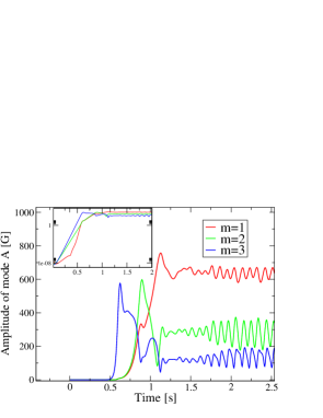
Figure 7: Time evolution of Fourier components of the azimuthal velocity. The shear layer is destabilized to non-axisymmetric modes via a Kelvin-Helmoltz type instability. In the linear phase, the $m=3$ azimuthal harmonic is the most unstable; the saturated state is dominated by $m=1$. Inset: the same evolution as a semilog plot.

Figure 7 shows the time evolution of azimuthal Fourier modes for $Rm=15$ and $S=11$. The initially axisymmetric MHD shear layer is destabilized to several azimuthal wavenumbers. In the linear phase, the $m=3$ mode clearly dominates. As the instability saturates, there is a cascade of energy towards lower azimuthal wavenumbers, and the nonlinear saturated state is strongly dominated by an oscillating $m=1$ mode. In the saturation phase, the thickness of the shear layer is increased, indicating that the instability saturates by modifying the shear profile.

Figure 8 shows the structure of these non-axisymmetric instabilities. In the linear phase, the structure is very similar to Kelvin-Helmoltz modes of the free shear layer, taking the form of columnar vortices transverse to the $(r,\phi)$ plane, independent of the axial direction and therefore symmetrical with respect to the equatorial plane. Note that the vortices spiral slightly in the prograde direction, as expected from a Kelvin-Helmoltz instability in cylindrical geometry transporting the angular momentum outward. Figure 8-top shows an isosurface of $25\%$ of the total shear $q$ in the flow. This illustrates how the rotational symmetry of the free shear layer is broken in the $\phi$ direction, the initially axisymmetric layer rolling up in a series of horizontal vortices by a mechanism similar to Kelvin-Helmoltz instabilities.

The structure of the magnetized shear layer strongly depends on the parameters. For a fixed value of the global rotation, the thickness $l$ of this shear layer scales with the Hartmann number as $l\sim r/\sqrt{M}$, a scaling similar to what is observed in spherical geometry. On the other hand, if the applied field is decreased after this shear layer has formed, the vertical extent of the shear layer is reduced, and eventually reaches a critical length where the Kelvin-Helmoltz instability does not occur. In our simulations, it appears that the vertical extent of the shear layer scales as $h\sim rM/\sqrt{Re}=r\sqrt{\Lambda}$. The condition $h\sim r$ thus gives the $\Lambda=1$, destabilization condition observed in our simulations: the non-axisymmetric modes develop by Kelvin-Helmoltz destabilization of the shear layer, provided that the layer is sufficiently extended in the vertical direction ($\Lambda>1$).

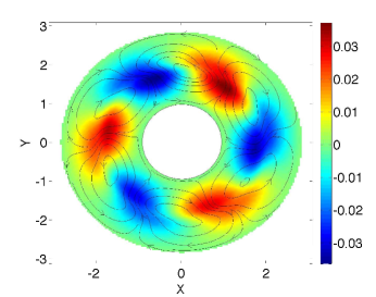
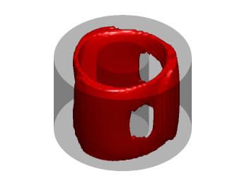
Figure 8: Structure of the non-axisymmetric instability for $Rm=15$, $S=11$. Top: Structure in the $r,\phi$ plane, for $z=H/4$. Non-axisymmetric component of the radial velocity $u_{r}$ in the equatorial plane during the linear phase. Bottom: $3D$ isosurface of the shear $q$. The mode consists of non-axisymmetric axial columnar modes, i.e. vortices in the $r,\phi$ plane (the axial component is much weaker) and mainly independent of the $z$-direction. Isosurface of the shear shows that these modes are essentially Kelvin-Helmoltz destabilization of the central magnetized shear layer.

V Comparison with laboratory experiments

Finally, we compare our numerical simulations to results obtained in the Princeton MRI experiment, where a similar setup is used (see Roach11 for more details on the experimental results mentioned here). Because of the very small magnetic Prandtl number of liquid metals ($Pm=Rm/Re\lesssim 10^{-5}$), it is very challenging to achieve fluid Reynolds numbers large enough to observe MRI in liquid-metal experiments. In Figure 2, the region of parameter space accessible to the Princeton experiment is indicated by the dashed square.

Our numerical simulations indicate that the magnetorotational instability should in theory be observable in the Princeton MRI experiment between $Rm=10$ and $Rm=15$; the latter corresponds to the maximum designed rotation rotation speed. Up to now, the maximum magnetic Reynolds number reached in the Princeton experiment is $Rm=9$, i.e. just below threshold. Our simulations suggest that the MRI should take the form of a gradual amplification of the residual Ekman flow. Since the experiment is still operating very close to the expected onset of the MRI, it is necessary to operate at higher $Rm$ to see MRI clearly. A further difficulty is that the saturation level is expected to be smaller in the experiment that in the simulations because of the $Re^{-1/4}$ scaling discussed above (Fig. 5).

By contrast, the shear layer instability is inductionless and should be observed at much smaller $Rm$. Figure 9 compares the numerical and experimental results for the horizontal structure of the mode. Non-axisymmetric modes have indeed been observed at very low rotation rates in the experiment, and these modes present several features identical to the instabilities reported here:

$\bullet$ First, the generation of non-axisymmetric modes in the experiment follows the marginal stability curve $\Lambda_{c}=1$, in agreement with our numerical prediction. Therefore, the experimental instabilities are also inductionless: they have been observed for rotation rates of the inner cylinder as small as $\Omega_{1}=0.05\,{\rm rad\,s^{-1}}$ ($Rm\ll 1$).

$\bullet$ The structure of the modes is very similar. Figure 9 compares the geometry of the modes in the ($r,\phi$) plane obtained in the experiment (bottom) and our simulations (top), for a case in which the dimensionless experimental parameters match the numerical ones except in magnetic Reynolds number. The similarity of the instability across two orders of magnitude in $Rm$ confirms its inductionless nature. In both cases, non-axisymmetric modes consist of equatorially symmetric vortices in the $(r,z)$ plane taking the form of an $m=1$ spiral mode sheared in the azimuthal direction. Note however that in the simulation, close to the instability onset, the modes spiral retrogradely in the midplane, but tend to be more prograde close to the rings (in agreement with the expected structure of a Kelvin-Helmoltz instability). This effect has not been observed in the experiment, where the spiral seems to be retrograde even relatively close to the endcaps. This could be due to the effect of the mean shear flow, or the secondary excitation of typical waves of the system, such as magneto-coriolis waves Nornberg10 . A prograde spiral is however expected sufficiently close to the endcaps, since it corresponds to an outward transport of the angular momentum by the Kelvin-Helmoltz instability.

$\bullet$ The time evolution is similar. In both numerical simulations and experiment, the saturated state is an $m=1$ mode rotating at a constant speed in the equatorial plane. Before reaching this $m=1$ mode, the experimental flow exhibits transient oscillations with different azimuthal symmetry, namely an $m=3$ followed by an $m=2$ mode. This is similar to the behavior of our numerical model, reported in Figure 7.

$\bullet$ In the experiment, non-axisymmetric modes are observed only when the difference of angular velocity between the inner ring and the outer ring is sufficiently large, and global rotation can stabilize the flow. These two features are also observed in our numerical simulations.

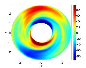
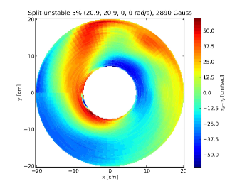
Figure 9: Comparison between numerical simulation (top) and ultrasound measurements Roach11 from the Princeton experiment (bottom). In both cases, inner rings corotate with the inner cylinder ($\Omega_{1}=\Omega_{3}$), outer rings and cylinder are at rest ($\Omega_{2}=0=\Omega_{4}$), $Re=1450$, and $\Lambda=1.6$. Simulation has $Rm=0.02$, and experiment, $Rm=0.002$. Figures show the non-axisymmetric component of the azimuthal velocity $U_{\phi}$ in the midplane, when the Shercliff layer is unstable. A very good agreement is obtained: in both cases, the saturated state consists of an $m=1$ spiral vortices rotating in the azimuthal direction. In the experiment, $U_{\phi}$ is obtained from two ultrasound probes measuring the radial profile of the velocity at two different azimuthal positions.

These several similarities strongly suggest that the non-axisymmetric modes observed in the Princeton MRI experiment are of the same nature as the ones reported in our numerical simulations, namely Kelvin-Helmoltz-type destabilization of a free shear layer created by the conjugate action of the axial magnetic field and the jump of angular velocity between the rotating rings at the endcaps. Note however that the magnetic boundary conditions at the endcaps are not exactly the same: our simulations use the idealized ’pseudo-vaccum’ boundary conditions given by eq.(5), whereas the endwalls are insulating in the Princeton experiment. Since insulating endwalls do not couple with magnetic field, the role of the electrical currents close to the endcaps in the establishment of the layer could be slightly different between experiments and numerics.

Interestingly, similar instabilities occur in spherical geometry, and could be involved in the oscillations observed in the Maryland experiment. More recently, similar rotating rings have also been used in the PROMISE experiment in order to obtain clearer observation of the Helical MRI, and non-axisymmetric $m=1$ modes have been reported. It would be interesting to see how these oscillations compare to the non-axisymmetric modes reported here.

VI Conclusion

In this article, we have reported three-dimensional numerical simulations of a magnetized cylindrical Taylor-Couette flow inspired by laboratory experiment aiming to observe the magnetorotational instability.

The influence of the boundaries on the MRI has been studied. We have shown that that the finite axial extent of the flow deeply modifies the nature of the bifurcation. In the presence of realistic boundaries, the MRI appears from a strongly imperfect supercritical pitchfork bifurcation, leading to several predictions for the observation of the instability in the laboratory. First, the transition to MRI is expected to gradually emerge from the residual recirculation driven by the top and bottom boundaries. Moreover, this Ekman flow directly modifies the structure of the instability by constraining the geometry of the mode, and different MRI modes can be observed depending on the hydrodynamical background state. As a consequence, the endcap rings of the Princeton experiment are not only useful to reduce the Ekman recirculation, but they can also be used to select different MRI modes.

In the second part of this study, we have reported the generation of non-axisymmetric modes when the applied magnetic field is sufficiently strong compared to the rotation (Elsasser number $>1$). Although they present some similarities with the MRI, these modes are of a very different nature: when the axial magnetic field is sufficiently strong, it generates a new free shear layer in the flow, by extending the jump of angular velocity between the inner and outer endcap rings into the bulk of the flow. When the shear is sufficiently strong, this layer is destabilized by non-axisymmetric modes of a Kelvin-Helmoltz type. It is interesting to note that this new instability shares several properties with the MRI: It transports angular momentum outward, it is stabilized at strong applied field, and a critical magnetic field is needed. However, these modes are inductionless, and therefore extend to very small $Rm$. This is an important difference from the classical MRI.

To finish, we have compared our numerical simulations to experimental results from the Princeton experiment. Good agreement is obtained at small $Rm$, where non-axisymmetric oscillations are also observed in the experiment. The marginal stability curve, the geometry of the mode, and the time evolution of these non-axisymmetric oscillations are similar to our numerical simulations. This indicates that the non-axisymmetric oscillations observed in the Princeton experiment could be related to the destabilization of the free shear layer (Shercliff layer) reported in the present numerical work.

To summarize, the present numerical study shows that the generation, structure, and saturation of the MRI are strongly modified by the presence of no-slip boundaries. In addition, new instabilities, similar to the MRI but inductionless, are generated in the presence of a strong magnetic field. This suggests that the observation of the magnetorotational instability in a laboratory experiment could be radically different from what is expected from local theory, or even axially-periodic Taylor-Couette simulations. However, careful comparisons between numerical simulations and experimental results could lead to a clear identification of the magnetorotational instability in the laboratory, and to a better understanding of the angular momentum transport.