Automatically Stable Discontinuous Petrov-Galerkin Methods for Stationary Transport Problems: Quasi-Optimal Test Space Norm

Abstract

We investigate the application of the discontinuous Petrov-Galerkin (DPG) finite element framework to stationary convection-diffusion problems. In particular, we demonstrate how the quasi-optimal test space norm can be utilized to improve the robustness of the DPG method with respect to vanishing diffusion. We numerically compare coarse-mesh accuracy of the approximation when using the quasi-optimal norm, the standard norm, and the weighted norm. Our results show that the quasi-optimal norm leads to more accurate results on three benchmark problems in two spatial dimensions. We address the problems associated to the resolution of the optimal test functions with respect to the quasi-optimal norm by studying their convergence numerically. In order to facilitate understanding of the method, we also include a detailed explanation of the methodology from the algorithmic point of view.

Keywords: convection-diffusion;   finite element method;   discontinuous Petrov-Galerkin;   numerical stability;   robustness;   automatic stabilization technique

1 Introduction

The purpose of this paper is to study the application of the discontinuous Petrov-Galerkin finite element methodology to convection-diffusion problems of the form

$$-\epsilon\Delta u+\mathbf{a}\cdot\boldsymbol{\nabla}u =f\quad\text{in $\Omega$}$$ (1)

$$u =g\quad\text{on $\partial\Omega$}$$

where $\Omega$ is a bounded two-dimensional domain, $\mathbf{a}$ is the flow velocity, $\epsilon$ is the diffusion parameter and $f$ represents a source term. The function $g$ determines the values of the solution $u$ on the boundary of the domain denoted by $\partial\Omega$. This equation is a basic model for various transport processes in nature and engineering. Typical applications include the movement of substances (dissolved nutrients, toxins) in the environment. Problem (1) may also be viewed as a stepping stone for designing numerical methods for more complex problems such as the Navier-Stokes equations for compressible and incompressible flows.

Construction of numerical solution schemes for (1) that can approximate convection dominated flows is known to be an inherently difficult task. Many scientists and engineers have addressed the problem and designed algorithms based on finite difference, finite volume, finite element and spectral approaches. In the context of the finite element method, the standard Ritz-Bubnov-Galerkin formulation is known to be deficient and various alternative formulations have been proposed in the literature, see for instance [29, 9, 35, 21, 22, 34, 27, 7, 12, 44, 8, 28, 10, 32].

The success of the traditional Galerkin finite element method in most structural problems is based on its best approximation property. This means that the difference between the finite element solution and the exact solution is minimized with respect to a norm induced by the strain energy product. Numerical issues arise when the best approximation property is lost. This happens, for instance, when the standard Galerkin method is applied to convective transport problems. In these problems, the system matrix associated to convection is not symmetric and numerical solutions tend to show spurious, non-physical oscillations unless the finite element mesh is heavily refined. It should be noted that the accuracy of the finite element method may also degrade in problems with symmetric system matrices. Thin-body problems of solid mechanics and wave propagation problems constitute typical examples. In these problems, the standard Galerkin method leads to non-physical solutions suffering from the phenomena of numerical locking (small thickness) and numerical dispersion (high wave number) unless an over-refined mesh is used.

To save computer resources, alternative formulations which produce reasonable approximations regardless of the mesh size have been developed. In the context of convective transport problems, a well-known method is the Streamline Upwind Petrov-Galerkin (SUPG) formulation, see [9, 36]. The method belongs to a larger class of stabilized finite element methods reviewed, for example, in [12, 25]. The stabilized finite element methods are geared mainly towards the classical $h$-version of the finite element method although some higher order formulations have been studied in [11, 24, 31, 4].

A new, general finite element framework has been developed by Demkowicz and Gopalakrishnan in [15, 16, 17]. This variational framework is of discontinuous Petrov-Galerkin (DPG) type and can be utilized, for example, to symmetrize non-symmetric problems by using the concept of optimal test functions similar to the early methodology developed by Barrett and Morton in [3], see also [21, 22, 39, 26, 38]. More precisely, if a fully discontinuous finite element space is used for the test functions, as in the DPG method of Bottasso et al. [5], the optimal test functions can be approximated locally in an enriched finite element space. The same procedure can also be used to compute local a posteriori error estimates to guide automatic adaptive mesh refinement as demonstrated in [19] in the context of convection-dominated diffusion problems and in [41] in the context of shell boundary layers.

Previous work in the DPG framework applied to Problem (1), has utilized adaptive mesh refinements [14, 19] to fully resolve fine scales (boundary and interior layers) in the solution. However, in engineering applications this is not always possible. In this work, we focus on the coarse-mesh accuracy of the DPG method. That is, we investigate how the effect of fine scales to the solution can be taken into account without resolving them by the trial space mesh. It should be noted that coarse-mesh accuracy is valuable even in the context of adaptive mesh refinement to avoid unnecessary mesh refinement.

We complement the earlier works [16, 19] by resolving the stable test function space with respect to the optimal (quasi-optimal) test space norm. The corresponding DPG method is expected to be uniformly stable with respect to vanishing diffusion, but the local problems for the test functions become singularly perturbed and therefore more difficult to solve. The main contribution of our study is to show how this problem can be approached by utilizing a carefully designed element sub-grid discretization. The present work is a continuation of our recent work [42, 43] and extends the earlier analysis in one space dimension to two dimensions.

The paper is structured to be self-contained and focused on bridging the theoretical framework to a practical understanding. Section 2 lays down the abstract functional analytic setup of the method. Then in Section 3, we specialize the theoretical framework to Problem (1) and introduce different test space norms. In Section 4, we re-explain the DPG framework from a purely algorithmic point of view in order to highlight the practical implications of the different choices of the test space norm. We provide details on how to construct the linear algebraic systems constituting the local optimal test functions. Numerical results are presented in Section 5 and the paper ends with conclusions and remarks in Section 6.

2 Automatically Stable DPG Framework

2.1 Background

The starting point of the formulation is an abstract variational statement of the form: Find $\mathbf{u}\in\mathcal{U}$ such that

$$\mathcal{B}(\mathbf{w},\mathbf{u})=\mathcal{L}(\mathbf{w}),\quad\forall\mathbf{w}\in\mathcal{W}$$ (2)

where the test function space $\mathcal{W}$ and the trial function space $\mathcal{U}$ are assumed to be Hilbert spaces under inner products $(\cdot,\cdot)_{\mathcal{W}}$ and $(\cdot,\cdot)_{\mathcal{U}}$ with the corresponding norms $||\cdot||_{\mathcal{W}}$ and $||\cdot||_{\mathcal{U}}$. We shall assume that the spaces are real because our application, Problem (1), deals only with real-valued functions.

If the spaces $\mathcal{W}$ and $\mathcal{U}$ are the same and $\mathcal{B}$ induces an inner product, then the standard Galerkin method delivers the best approximation of the exact solution in the corresponding norm known as the energy norm. In the case of Problem (1) the conventional weak formulation is associated with the bilinear and linear forms

$$\mathcal{B}(v,u)=\int_{\Omega}\left(\epsilon\boldsymbol{\nabla}v\cdot\boldsymbol{\nabla}u+v(\mathbf{a}\cdot\boldsymbol{\nabla}u)\right)\,\mathrm{d}\Omega,\quad\mathcal{L}(v)=\int_{\Omega}vf\,\mathrm{d}\Omega$$ (3)

Here $\mathcal{B}$ does not induce an inner product because the second term is not symmetric. Consequently the best approximation property in the energy norm is lost together with numerical stability, see [9, 33]. This has motivated the use of the Petrov-Galerkin method, where the combination of specially engineered test functions with added stabilization terms in the variational formulation, has improved the numerical approximations considerably. The DPG method discussed here restores the best approximation property by the computation of a special set of test functions for given trial functions that produce a symmetric positive-definite algebraic system when substituted in the bilinear form. The method can be explored from many different perspectives. It may be viewed as an automatic apparatus designed for guaranteeing the famous inf-sup condition of the Babuška-Brezzi theory of discrete stability, see [1, 6], or it may be interpreted as a generalized least squares method, see [17]. We treat the methodology as a numerical construction which generates a true inner-product structure for any well-posed variational problem.

2.2 Petrov-Galerkin Method with Optimal Test Functions

The goal is to find a linear operator $\mathbf{T}$ which maps the trial function space $\mathcal{U}$ to the test function space $\mathcal{W}$ such that

$$\mathcal{B}(\mathbf{T}\mathbf{v},\mathbf{u})=\mathcal{A}(\mathbf{v},\mathbf{u})\quad\forall\mathbf{v},\mathbf{u}\in\mathcal{U}$$ (4)

where $\mathcal{A}(\mathbf{v},\mathbf{u})$ is a symmetric coercive bilinear form on $\mathcal{U}\times\mathcal{U}$. If $\{\mathbf{e}_{1},\mathbf{e}_{2},\ldots,\mathbf{e}_{n}\}$ denotes a set of trial functions that spans a subspace $\mathcal{U}_{n}$ of $\mathcal{U}$, then the use of the test functions $\mathbf{T}\mathbf{e}_{i}$ in the Petrov-Galerkin method

$$\mathcal{B}(\mathbf{T}\mathbf{e}_{i},\mathbf{u}_{n})=\mathcal{L}(\mathbf{T}\mathbf{e}_{i}),\quad i=1,\dots,n$$ (5)

defines $\mathbf{u}_{n}$ as the orthogonal projection of the exact solution $\mathbf{u}$ onto the trial space $\mathcal{U}_{n}$ with respect to the inner product $\mathcal{A}(\cdot,\cdot)$:

$$\mathcal{A}(\mathbf{v}_{n},\mathbf{u}-\mathbf{u}_{n})=0\quad\forall\mathbf{v}_{n}\in\mathcal{U}_{n}$$

In other words, $\mathbf{u}_{n}$ is the best approximation of $\mathbf{u}$ in $\mathcal{U}_{n}$ in the corresponding ‘energy’ norm, that is,

$$|||\mathbf{u}-\mathbf{u}_{n}|||_{\mathcal{U}}\leq|||\mathbf{u}-\mathbf{v}|||_{\mathcal{U}}\quad\forall\mathbf{v}\in\mathcal{U}_{n}$$

where

$$|||\mathbf{u}|||_{\mathcal{U}}=\sqrt{\mathcal{A}(\mathbf{u},\mathbf{u})}\quad\forall\mathbf{u}\in\mathcal{U}$$

A canonical way to define the trial-to-test operator $\mathbf{T}:\mathcal{U}\rightarrow\mathcal{W}$ is to define $\mathbf{T}\mathbf{u}\in\mathcal{W}$ through the variational equality

$$(\mathbf{w},\mathbf{T}\mathbf{u})_{\mathcal{W}}=\mathcal{B}(\mathbf{w},\mathbf{u})\quad\forall\,\mathbf{w}\in\mathcal{W}$$ (6)

so that we have

$$\mathcal{B}(\mathbf{T}\mathbf{v},\mathbf{u})=(\mathbf{T}\mathbf{v},\mathbf{T}\mathbf{u})_{\mathcal{W}}$$

and thus achieve our goal with

$$\mathcal{A}(\mathbf{v},\mathbf{u})=(\mathbf{T}\mathbf{v},\mathbf{T}\mathbf{u})_{\mathcal{W}},\quad|||\mathbf{u}|||_{\mathcal{U}}=||\mathbf{T}\mathbf{u}||_{\mathcal{W}}$$ (7)

2.3 Localization

For each trial function $\mathbf{e}_{i}$, $i=1,\ldots,n$, Equation (6) constitutes an auxiliary, infinite-dimensional variational problem associated with the test function space $\mathcal{W}$. The standard Galerkin method may be used to approximate solutions to Equation (6). However, for typical variational formulations, like for the one corresponding to the forms of (3), Equation (6) is from the computational perspective at least as ‘heavy’ as the original problem.

The new insight of Demkowicz and Gopalakrishnan, see [16], was to formulate the variational problem (2) in an ultra-weak hybrid form in such a way that the test function space $\mathcal{W}$ becomes fully discontinuous on a partitioning of $\Omega$ into elements $\{K_{1},K_{2},\ldots,K_{N}\}$:

$$\mathcal{W}=\{\mathbf{w}:\mathbf{w}\!\!\mid_{K}\in\mathcal{W}(K)\;\text{for every element $K$}\}$$

As long as the inner product $(\cdot,\cdot)_{\mathcal{W}}$ does not couple test functions defined on individual elements, the auxiliary problems defined by Equation (6) can be solved locally at the element level. The localized version of the problem can be written in terms of the broken forms

$$(\cdot,\cdot)_{\mathcal{W}}=\sum_{K}(\cdot,\cdot)_{\mathcal{W}(K)}^{2},\quad\mathcal{B}(\cdot,\cdot)=\sum_{K}\mathcal{B}_{K}(\cdot,\cdot)$$

which allows the global problem (6) to be written as finding $\mathbf{T}\mathbf{u}\in\mathcal{W}(K)$ such that

$$(\mathbf{w},\mathbf{T}\mathbf{u})_{\mathcal{W}(K)}=\mathcal{B}_{K}(\mathbf{w},\mathbf{u})\quad\forall\mathbf{w}\in\mathcal{W}(K)$$ (8)

This problem may then be solved approximately using the standard Galerkin method in an enriched finite element space $\mathcal{W}_{\tilde{n}}(K)\subset\mathcal{W}(K)$, that is, find $\tilde{\mathbf{T}}\mathbf{u}\in\mathcal{W}_{\tilde{n}}(K)$ such that

$$(\mathbf{w},\tilde{\mathbf{T}}\mathbf{u})_{\mathcal{W}(K)}=\mathcal{B}_{K}(\mathbf{w},\mathbf{u})\quad\forall\mathbf{w}\in\mathcal{W}_{\tilde{n}}(K)$$ (9)

2.4 Well-posedness and Robustness

The above construction can be carried out provided that the original variational problem (2) is well-posed, that is, provided that the bilinear form $\mathcal{B}(\mathbf{w},\mathbf{u})$ satisfies the conditions of the Babuška-Necas-Nirenberg Theorem, which are (see [1] and [6, 13])

$$\mathcal{B}(\mathbf{w},\mathbf{u})\leq C_{1}||\mathbf{w}||_{\mathcal{W}}||\mathbf{u}||_{\mathcal{U}}\quad\forall\mathbf{w}\in\mathcal{W},\;\mathbf{u}\in\mathcal{U}$$ (10)

$$\sup_{\mathbf{u}\in\mathcal{U}}\frac{\mathcal{B}(\mathbf{w},\mathbf{u})}{||\mathbf{u}||_{\mathcal{U}}}\geq C_{2}||\mathbf{w}||_{\mathcal{W}}$$ (11)

$$\sup_{\mathbf{w}\in\mathcal{W}}\frac{\mathcal{B}(\mathbf{w},\mathbf{u})}{||\mathbf{w}||_{\mathcal{W}}}\geq C_{3}||\mathbf{u}||_{\mathcal{U}}$$ (12)

The first condition implies that the right hand side of Equation (6) is a bounded linear functional in $\mathcal{W}$ for every $\mathbf{u}\in\mathcal{U}$. Therefore $\mathbf{T}\mathbf{u}\in\mathcal{W}$ exists and is unique.

The second condition guarantees that the mapping $\mathbf{T}$ is surjective, that is, every $\mathbf{w}\in\mathcal{W}$ can be expressed in the form $\mathbf{w}=\mathbf{T}\mathbf{u}$ for some $\mathbf{u}\in\mathcal{U}$. Namely, if this was not the case, there would exist a non-zero $\tilde{\mathbf{w}}\in\mathcal{W}$ such that $(\tilde{\mathbf{w}},\mathbf{T}\mathbf{u})_{\mathcal{W}}=0$ for all $\mathbf{u}\in\mathcal{U}$. But then also

$$\mathcal{B}(\tilde{\mathbf{w}},\mathbf{u})=0\quad\forall\mathbf{u}\in\mathcal{U}$$

by Equation (6) so that Equation (11) implies $\tilde{\mathbf{w}}=\boldsymbol{0}$, which is a contradiction.

Finally, the coercivity of the bilinear form $\mathcal{A}$ follows from condition (12). To see this, we recall that the norm of an element in a Hilbert space $\mathcal{H}$ can be computed by duality as

$$||\mathbf{u}||_{\mathcal{H}}=\sup_{\mathbf{v}\in\mathcal{H}}\frac{(\mathbf{v},\mathbf{u})_{\mathcal{H}}}{||\mathbf{v}||_{\mathcal{H}}}$$ (13)

so that the energy norm can be expressed as

$$|||\mathbf{u}|||_{\mathcal{U}}=\sup_{\mathbf{w}\in\mathcal{W}}\frac{(\mathbf{w},\mathbf{T}\mathbf{u})_{\mathcal{W}}}{||\mathbf{w}||_{\mathcal{W}}}=\sup_{\mathbf{w}\in\mathcal{W}}\frac{\mathcal{B}(\mathbf{w},\mathbf{u})}{||\mathbf{w}||_{\mathcal{W}}}$$

Now Equation (12) implies that

$$\mathcal{A}(\mathbf{u},\mathbf{u})\geq C_{3}^{2}||\mathbf{u}||_{\mathcal{U}}^{2}\quad\forall\,\mathbf{u}\in\mathcal{U}$$

The characteristics of the energy norm depend on the values of the constants $C_{1}$ and $C_{3}$ which in turn typically depend on the physical parameters and the problem geometry. As a result the Petrov-Galerkin method (5) may not be robust, that is, uniformly accurate with respect to the parameter values of a particular physical problem that is being modeled, see [2]. However, the parametric dependence can be removed completely from the bilinear form $\mathcal{A}(\cdot,\cdot)$ by using a special norm for the test function space in (6). This norm is referred to as the optimal test space norm in the DPG literature, see for instance [48], and can be defined as

$$|||\mathbf{w}|||_{\mathcal{W}}=||\mathbf{T}^{*}\mathbf{w}||_{\mathcal{U}}$$ (14)

where $\mathbf{T}^{*}:\mathcal{W}\rightarrow\mathcal{U}$ is a linear mapping such that

$$(\mathbf{T}^{*}\mathbf{w},\mathbf{u})_{\mathcal{U}}=\mathcal{B}(\mathbf{w},\mathbf{u})\quad\forall\mathbf{u}\in\mathcal{U}$$

Equation (14) defines a proper norm in $\mathcal{W}$ again under the assumption that the variational problem is well-posed. Namely, the utilization of the duality argument (13), and conditions (10)–(11) show that

$$C_{2}||\mathbf{w}||_{\mathcal{W}}\leq||\mathbf{T}^{*}\mathbf{w}||_{\mathcal{U}}\leq C_{1}||\mathbf{w}||_{\mathcal{W}}$$

that is, $|||\cdot|||_{\mathcal{W}}$ is an equivalent norm to $||\cdot||_{\mathcal{W}}$.

Finally, condition (12) implies that $\mathbf{T}^{*}$ is surjective so that a subsequent application of the duality argument (13) yields

$$|||\mathbf{u}|||_{\mathcal{U}}=\sup_{\mathbf{w}\in\mathcal{W}}\frac{\mathcal{B}(\mathbf{w},\mathbf{u})}{|||\mathbf{w}|||_{\mathcal{W}}}=\sup_{\mathbf{w}\in\mathcal{W}}\frac{(\mathbf{T}^{*}\mathbf{w},\mathbf{u})_{\mathcal{U}}}{||\mathbf{T}^{*}\mathbf{w}||_{\mathcal{U}}}=\sup_{\mathbf{v}\in\mathcal{U}}\frac{(\mathbf{v},\mathbf{u})_{\mathcal{U}}}{||\mathbf{v}||_{\mathcal{U}}}=||\mathbf{u}||_{\mathcal{U}}$$ (15)

Thus, the introduction of (14) allows us to obtain a problem for each trial function which yields a robust method (convergent in the $||\cdot||_{\mathcal{U}}$ norm as stated in (15)). This guaranteed best approximation property is what leads us to call the norm induced by Equation (14) optimal. As we will observe in the proceeding Section, the ultra-weak approach allows the expression of the optimal test space norm to be deduced directly from the bilinear form. Additionally, the leading terms can be expressed in a closed, localizable form.

3 DPG Method for the Convection-Diffusion Problem

In this section we follow [16, 18] and derive an explicit DPG variational formulation of the convection-diffusion equation. The ultra-weak DPG variational form of the problem is associated initially to a partitioning of $\Omega$ into elements denoted by $\Omega_{h}$. We will refer to the collection of all edges in the mesh as $\partial\Omega_{h}=\cup_{K}\partial K$. We will use the standard notation where $L_{2}(\Omega)$ and $\boldsymbol{L}_{2}(\Omega)$ denote the spaces of square-integrable scalar- and vector-valued functions over $\Omega$, respectively. Moreover, $H^{1}(\Omega)$ and $\boldsymbol{H}(\mathrm{div},\Omega)$ stand for the subspaces consisting of functions with square-integrable derivatives:

$$H^{1}(\Omega) =\{v\in L_{2}(\Omega)\;:\;\boldsymbol{\nabla}v\in L_{2}(\Omega)\}$$

$$\boldsymbol{H}(\mathrm{div},\Omega) =\{\boldsymbol{\tau}\in\boldsymbol{L}_{2}(\Omega)\;:\;\boldsymbol{\nabla}\cdot\boldsymbol{\tau}\in L_{2}(\Omega)\}$$

3.1 Derivation of the Hybrid Ultra-Weak Variational Form

The procedure begins by rewriting the second-order partial differential equation in (1) as a pair of first-order equations

$$\epsilon^{-1}\boldsymbol{\sigma} =-\boldsymbol{\nabla}u$$ (16)

$$\boldsymbol{\nabla}\cdot\boldsymbol{\sigma}+\mathbf{a}\cdot\boldsymbol{\nabla}u =f$$

Here we have chosen to define $\boldsymbol{\sigma}$ as the diffusive flux in order to be consistent with the above cited references. Other option would be to include the advective flux $\mathbf{a}u$ in the first equation defining $\boldsymbol{\sigma}$ as in our earlier works [42, 43]. In our experience, the difference between the two approaches appears to be mostly cosmetic. In this work we will assume that the ambient fluid is incompressible so that $\boldsymbol{\nabla}\cdot\mathbf{a}=0$ and that the problem is formulated in a dimensionless form scaled such that $\left|\mathbf{a}\right|\sim 1$.

Upon multiplying the first and second equations in (16) by a vector-valued test function $\boldsymbol{\tau}$ and a scalar-valued test function $v$, respectively, and integrating by parts element-wise, we obtain the following bilinear and linear forms corresponding to the abstract variational statement (2)

$$\mathcal{B}(\mathbf{w},\mathbf{u}) =(\epsilon^{-1}\boldsymbol{\tau}-\boldsymbol{\nabla}v,\boldsymbol{\sigma})_{\Omega_{h}}-(\boldsymbol{\nabla}\cdot\boldsymbol{\tau}+\mathbf{a}\cdot\boldsymbol{\nabla}v,u)_{\Omega_{h}}+\langle\boldsymbol{\tau}\cdot\mathbf{n},\hat{u}\rangle_{\partial\Omega_{h}}+\langle\hat{\sigma}_{n},v\rangle_{\partial\Omega_{h}}$$ (17)

$$\mathcal{L}(\mathbf{w}) =(v,f)_{\Omega_{h}}$$

Here $\mathbf{n}$ denotes the outward unit normal on each element edge and $\hat{\sigma}_{n}$ corresponds to the (outer) normal component of the total flux $(\boldsymbol{\sigma}+\mathbf{a}u)\cdot\mathbf{n}$. Moreover, the test function is denoted by $\mathbf{w}=(\boldsymbol{\tau},v)$ and the trial function by $\mathbf{u}=(\boldsymbol{\sigma},u,\hat{u},\hat{\sigma}_{n})$. For smooth functions, the notations $(\cdot,\cdot)_{\Omega_{h}}$ and $\langle\cdot,\cdot\rangle_{\partial\Omega_{h}}$ stand for the element-wise computed inner products

$$(f,g)_{\Omega_{h}}=\sum_{K\in\Omega_{h}}\int_{K}fg\,\mathrm{d}\Omega,\quad\langle f,g\rangle_{\partial\Omega_{h}}=\sum_{K\in\Omega_{h}}\int_{\partial K}fg\,\mathrm{d}s$$

The element integrals $(\cdot,\cdot)_{\Omega_{h}}$ in Equation (17) make sense provided that $\boldsymbol{\sigma},u,\boldsymbol{\tau},v$ as well as $\boldsymbol{\nabla}\cdot\boldsymbol{\tau}$ and $\boldsymbol{\nabla}v$ are square integrable over each $K$. Thus, the test function space is defined as the broken space

$$\mathcal{W}=\boldsymbol{H}(\mathrm{div},\Omega_{h})\times H^{1}(\Omega_{h})$$ (18)

where

$$\boldsymbol{H}(\mathrm{div},\Omega_{h}) =\{\boldsymbol{\tau}\in\boldsymbol{L}_{2}(\Omega)\;:\;\boldsymbol{\nabla}\cdot\boldsymbol{\tau}\in L_{2}(K)\quad\forall K\in\Omega_{h}\}$$

$$H^{1}(\Omega_{h}) =\{v\in L_{2}(\Omega)\;:\;\boldsymbol{\nabla}v\in L_{2}(K)\quad\forall K\in\Omega_{h}\}$$

In the general case, the interface action $\langle\cdot,\cdot\rangle_{\partial\Omega_{h}}$ in (17) must be interpreted as an appropriate duality pairing between suitable generalized function spaces defined on $\partial K$. The right setting can be deduced from the theory of trace operators naturally associated to the spaces $\boldsymbol{H}(\mathrm{div},K)$ and $H^{1}(K)$. These spaces are formally denoted by $H^{-1/2}(\partial K)$ and $H^{1/2}(\partial K)$ for the normal trace $\boldsymbol{\tau}\!\cdot\mathbf{n}\mid_{\partial K}$ and the standard trace $v\!\mid_{\partial K}$, respectively.

This leads to the definition of the trial function space as

$$\mathcal{U}=\boldsymbol{L}^{2}(\Omega)\times L^{2}(\Omega)\times H_{D}^{1/2}(\partial\Omega_{h})\times H^{-1/2}(\partial\Omega_{h})$$ (19)

where the spaces for the interface variables $\hat{u}$ and $\hat{\sigma}_{n}$ are defined as

$$H_{D}^{1/2}(\partial\Omega_{h}) =\{v\!\mid_{\partial\Omega_{h}}\;:\;v\in H_{D}^{1}(\Omega)\}$$

$$H^{-1/2}(\partial\Omega_{h}) =\{\boldsymbol{\eta}\!\mid_{\partial\Omega_{h}}\;:\;\boldsymbol{\eta}\in H(\mathrm{div},\Omega)\}$$

Here $H_{D}^{1}(\Omega)$ refers to the subspace of $H^{1}(\Omega)$ encompassing the Dirichlet boundary condition $u=g$ on $\partial\Omega$. The topology of the numerical trace spaces can be characterized for instance by using the extensions with minimal norm:

$$||\hat{u}||_{H^{1/2}(\partial\Omega_{h})} =\{\inf||v||_{H^{1}(\Omega)}\;:\;v\in H^{1}(\Omega)\;\text{such that}\;v\!\mid_{\partial\Omega_{h}}=\hat{u}\}$$

$$||\hat{\sigma}_{n}||_{H^{-1/2}(\partial\Omega_{h})} =\{\inf||\boldsymbol{\eta}||_{\boldsymbol{H}(\mathrm{div},\Omega)}\;:\;\boldsymbol{\eta}\in\boldsymbol{H}(\mathrm{div},\Omega)\;\text{such that}\;\boldsymbol{\eta}\cdot\mathbf{n}\!\mid_{\partial\Omega_{h}}=\hat{\sigma}_{n}\}$$

More details regarding these definitions can be found from [18]. For our purposes it suffices to note that piecewise polynomial functions in $H_{D}^{1/2}(\partial\Omega_{h})$ must be globally continuous on $\partial\Omega_{h}$ whereas discontinuities at the vertices of $\Omega_{h}$ are allowed in the space $H^{-1/2}(\partial\Omega_{h})$.

3.2 Finite Element Trial Spaces

We refer to $P_{t}$ as the set of polynomials of degree lower or equal to $t$ and to the corresponding tensor product family by $Q_{p_{x},p_{y}}=P_{p_{x}}\times P_{p_{y}}$ and set $Q_{p}=Q_{p,p}$. The trial space is defined then as

$$\mathcal{U}_{n}=S_{h}^{2}\times S_{h}\times M_{h}\times N_{h}$$

where

$$S_{h} =\{v\in L_{2}(\Omega):v\!\!\mid_{K}\;\in Q_{p}\;\text{for every element $K$}\}$$

$$M_{h} =\{v\in H_{D}^{1}(\Omega):v\!\!\mid_{E}\;\in P_{p+1}\;\text{for every edge $E$}\}$$

$$N_{h} =\{v:v\!\!\mid_{E}\;\in P_{p}\;\text{for every edge}\;E\}$$

In this work we use the Bernstein polynomials as a basis for $P_{t}$. The $t+1$ basis polynomials are defined as

$$B_{i,t}(x)=\binom{t}{i}x^{i}(1-x)^{t-i},\quad i=0,1,\ldots,t$$

3.3 Localization in the Convection-Diffusion Problem

Upon selection of a norm $||\cdot||_{\mathcal{W}}^{2}=(\cdot,\cdot)_{\mathcal{W}}$ for the broken test function space $\mathcal{W}$ defined in (18), a precise form of the localized auxiliary problem (8) is obtained. This problem is solved approximately using the standard Galerkin method and an enriched finite element space defined on each element $K$. We will associate this space to a sub-partitioning of $K$ into elements $\{\tilde{K}_{1},\ldots,\tilde{K}_{\tilde{N}}\}$.

More precisely, we define an $\boldsymbol{H}(\mathrm{div},K)\times H^{1}(K)$-conforming finite element space for the test functions as

$$\mathcal{W}_{\tilde{n}}(K)=\mathcal{T}_{\tilde{h}}\times\mathcal{V}_{\tilde{h}}$$

where

$$\mathcal{T}_{\tilde{h}} =\{\boldsymbol{\tau}\in H(\mathrm{div},K):\boldsymbol{\tau}\!\!\mid_{\tilde{K}}\in Q_{\tilde{p}+1,\tilde{p}}\times Q_{\tilde{p},\tilde{p}+1}\;\text{for every sub-element $\tilde{K}$}\}$$

$$\mathcal{V}_{\tilde{h}} =\{v\in H^{1}(K):v\!\!\mid_{\tilde{K}}\in Q_{\tilde{p}}\;\text{for every sub-element $\tilde{K}$}\}$$

Here we denote $\tilde{p}=p+\Delta p$ so that the level of enrichment is controlled by both the number of sub-elements $\tilde{N}$ and the increment in the order of approximation $\Delta p$. In what follows, we will describe three different choices of the test space norm and discuss appropriate enrichments for resolving the corresponding test functions.

The Standard Test Space Norm

A norm known as the standard norm, or mathematician’s norm, may be constructed by composing the natural norms of the spaces $\boldsymbol{H}(\mathrm{div},\Omega_{h})$ and $H^{1}(\Omega_{h})$ as in

$$||\mathbf{w}||_{\mathrm{SN}}^{2}=||\boldsymbol{\nabla}\cdot\boldsymbol{\tau}||_{\Omega_{h}}^{2}+||\boldsymbol{\tau}||_{\Omega_{h}}^{2}+||\boldsymbol{\nabla}v||_{\Omega_{h}}^{2}+||v||_{\Omega_{h}}^{2}$$

This choice leads to two decoupled, standard variational problems for $\boldsymbol{\tau}$ and $v$ over each element $K$ which can be solved sufficiently accurately by using an enriched finite element space with $\Delta p=2$ and $\tilde{N}=1$, see [16].

The Weighted Test Space Norm

While the standard norm provides a local problem that is easy to solve, it leads to approximations of $u$ that underestimate the true values considerably. It was determined in [19], that the use of a special weighting of the norm near the inflow boundary could improve the accuracy. The original version of the weighted norm, as introduced in [19], is based directly on the standard norm and reads

$$||\mathbf{w}||^{2}_{\mathrm{WN}}=||\boldsymbol{\nabla}\cdot\boldsymbol{\tau}||_{\Omega_{h},\beta}^{2}+||\boldsymbol{\tau}||_{\Omega_{h},\beta}^{2}+||\boldsymbol{\nabla}v||_{\Omega_{h},\beta}^{2}+||v||_{\Omega_{h},\beta}^{2}$$

where $\beta$ is a piecewise constant norm weight such that

$$\beta(\mathbf{x})=\begin{cases}\gamma,&\text{if $d(\mathbf{x},\Gamma^{-})\leq\delta$ \& $d(\mathbf{x},\Gamma^{+})\geq\delta$}\\ 1,&\text{otherwise}\end{cases}$$

where $d(\mathbf{x},\Gamma^{-})$ and $d(\mathbf{x},\Gamma^{+})$ stand for the (normal) distances between the point $\mathbf{x}$ and the inflow and outflow/no-flow boundaries, respectively. These are defined as

$$\Gamma^{-} =\{\mathbf{x}\in\partial\Omega:\mathbf{a}\cdot\mathbf{n}<0\}$$

$$\Gamma^{+} =\{\mathbf{x}\in\partial\Omega:\mathbf{a}\cdot\mathbf{n}\geq 0\}$$

It should be noted that different refined variants of the weighted norm have been recently introduced and studied in [20]. These refinements have resemblance to the quasi-optimal norm introduced next.

The Quasi-Optimal Test Space Norm

While the weighted test space norm resolves some of the deficiencies of the standard norm, the approach is not optimal in the sense of the DPG theory as outlined in Section 2.4. In contrast to the weighted test space norm, we describe here the optimal test space norm (14). However, the true optimal norm leads to a series of global problems so that some numerical modifications are necessary to make the approach suitable for practical computations. This way we arrive to a quasi-optimal test space norm which retains the essential features of the optimal test space norm but is localizable.

Let the trial space norm be the natural norm arising from the definition (19)

$$||\mathbf{u}||_{\mathcal{U}}=\left\{||\boldsymbol{\sigma}||_{L_{2}(\Omega)}^{2}+||u||_{L_{2}(\Omega)}^{2}+||\hat{u}||_{H^{1/2}(\partial\Omega_{h})}^{2}+||\hat{\sigma}_{n}||_{H^{-1/2}(\partial\Omega_{h})}^{2}\right\}^{1/2}$$

Thus, using the definition (17) of the bilinear form, we can express the optimal test space norm (14) as

$$|||\mathbf{w}|||_{\mathcal{W}}^{2}=||\epsilon^{-1}\boldsymbol{\tau}-\boldsymbol{\nabla}v||_{\Omega_{h}}^{2}+||\boldsymbol{\nabla}\cdot\boldsymbol{\tau}+\mathbf{a}\cdot\boldsymbol{\nabla}v||_{\Omega_{h}}^{2}+||[\boldsymbol{\tau}\cdot\mathbf{n}]||_{\partial\Omega_{h}}^{2}+||[v\mathbf{n}]||_{\partial\Omega_{h}}^{2}$$

where

$$||[\boldsymbol{\tau}\cdot\mathbf{n}]||_{\partial\Omega_{h}}=\sup_{\hat{u}\in H_{D}^{1/2}(\partial\Omega_{h})}\frac{\langle\hat{u},\boldsymbol{\tau}\cdot\mathbf{n}\rangle_{\partial\Omega_{h}}}{||\hat{u}||_{H^{1/2}(\partial\Omega_{h})}},\quad||[v\mathbf{n}]||_{\partial\Omega_{h}}=\sup_{\hat{\sigma}_{n}\in H^{-1/2}(\partial\Omega_{h})}\frac{\langle v,\hat{\sigma}_{n}\rangle_{\partial\Omega_{h}}}{||\hat{\sigma}_{n}||_{H^{-1/2}(\partial\Omega_{h})}}$$

The last two terms can be made more precise, see [18], but the important point is that they involve the ‘jumps’ of $\boldsymbol{\tau}$ and $v$ along the inter-element boundaries and therefore prevent the element-wise computation of the optimal test functions. However, a localizable variant of the optimal norm may obtained simply by dropping these terms and adding an integral contribution of $v$, so as to remove the ‘zero-energy mode’ $(\boldsymbol{\tau},v)=(\boldsymbol{0},\mathrm{const.})$. This leads us to the so-called quasi-optimal test space norm

$$||\mathbf{w}||_{\mathrm{QON}}^{2}=||\epsilon^{-1}\boldsymbol{\tau}-\boldsymbol{\nabla}v||_{\Omega_{h}}^{2}+||\boldsymbol{\nabla}\cdot\boldsymbol{\tau}+\mathbf{a}\cdot\boldsymbol{\nabla}v||_{\Omega_{h}}^{2}+\alpha_{1}||\boldsymbol{\tau}||_{\Omega_{h}}^{2}+\alpha_{2}||v||_{\Omega_{h}}^{2}$$ (20)

where $\alpha_{1}\geq 0$ and $\alpha_{2}>0$ are numerical regularization parameters to be chosen. Notice that while the addition of a contribution of $||\boldsymbol{\tau}||_{\Omega_{h}}^{2}$ is not necessary, we have observed that a proper regularization of $\boldsymbol{\tau}$ improves the accuracy of the final approximation. In our algorithm we choose $\alpha_{1}=\epsilon^{-3/2}$ and $\alpha_{2}=1$.

A critical issue in the application of the quasi-optimal norm (20) is that the auxiliary problems for the test functions become singularly perturbed. This was explored in the one-dimensional case in [42, 43] where a specially designed sub-grid mesh was employed to resolve the potential boundary layers in the test functions. To extend the idea to two spatial dimensions, we observe that the strong form of the problem (8) associated to the quasi-optimal test space norm (20) takes the form

$$\left\{\begin{aligned} -\boldsymbol{\nabla}(\boldsymbol{\nabla}\cdot\boldsymbol{\tau})+(\epsilon^{-2}+\alpha_{1})\boldsymbol{\tau}-\boldsymbol{\nabla}(\mathbf{a}\cdot\boldsymbol{\nabla}v)-\epsilon^{-1}\boldsymbol{\nabla}v&=\varepsilon^{-1}\boldsymbol{\sigma}+\boldsymbol{\nabla}u\\ -\Delta v-\mathbf{a}\cdot\boldsymbol{\nabla}(\mathbf{a}\cdot\boldsymbol{\nabla}v)+\alpha_{2}v-\mathbf{a}\cdot\boldsymbol{\nabla}(\boldsymbol{\nabla}\cdot\boldsymbol{\tau})+\epsilon^{-1}\boldsymbol{\nabla}\cdot\boldsymbol{\tau}&=\boldsymbol{\nabla}\cdot\boldsymbol{\sigma}+\mathbf{a}\cdot\boldsymbol{\nabla}u\end{aligned}\right.$$ (21)

in every $K$. Notice that the system (21) corresponds to the Euler-Lagrange equations for the variational problem (6) and is accompanied with inhomogeneous natural boundary conditions involving also the interface variables $\hat{\sigma}_{n}$ and $\hat{u}$.

While a detailed regularity and asymptotic analysis of the system (21) is out of the scope of this paper, a preliminary examination of the system when $K=(0,1)\times(0,1)$ and $\mathbf{a}=(1,0)$ or $\mathbf{a}=(0,1)$ reveals that the solution may exhibit regular, exponential boundary layers behaving like

$$e^{-\lambda x_{1}},\quad e^{-\lambda(1-x_{1})},\quad e^{-\lambda x_{2}},\quad e^{-\lambda(1-x_{2})}$$

where the characteristic exponent is given by $\lambda=\epsilon^{-1}\sqrt{1+\alpha_{1}\epsilon^{2}}$. Notice that when $\alpha_{1}=\epsilon^{3/2}$, we have $\lambda=\epsilon^{-1}+\mathcal{O}(\epsilon^{-1/2})$. To account for these features in the automatic computation of the optimal test functions, we employ a layer-adapted Shishkin mesh on each $K$ as shown in Figure 1. Such meshes are commonly used in the approximation of singularly perturbed problems, see [37, 46]. We follow a strategy which consists of adding one layer of ’needle’ elements of width $\mathcal{O}(\tilde{p}\epsilon)$ near the boundary and has been proven to be optimal in the context of the $hp$-version of FEM for reaction-diffusion equations, see [45, 47, 40].

We emphasize that the sub-grid discretization is needed only when using the quasi-optimal test space norm. Failure to address the fine-scale features of the corresponding test functions (here using the sub-grid) degrades the accuracy of the final solution and dissipates all benefits of the quasi-optimal test norm.

Figure 1: A $3\times 3$ Shishkin mesh to resolve the boundary layers of the optimal test functions.

4 Algorithmic Considerations

At the high level, the DPG method with optimal test functions is similar to the standard finite element method detailed in Algorithm 1. Initially, the mesh information is input and mappings from the local stiffness matrix to the global matrix are determined. After this, we loop over the elements and form the element contributions to the global stiffness matrix and load vector. The main conceptual difference between the DPG method and standard FEM is the following: the local stiffness matrix will be computed as a by-product of computing the optimal test functions. Another difference is that, because of the hybridization, the trial spaces are non-standard and require some specialized handling. The remaining portion of this section will describe both differences in more detail. For a review of standard FEM implementation, see [30, 14].

Algorithm 1 The DPG finite element method with optimal test functions

1:Initialize mesh

2:Compute all local to global maps

3:for all elements in mesh do

4:     Compute local contributions $\mathbf{K}_{\ell},\mathbf{F}_{\ell}$ using OptimalTestFunctions (Algorithm 2)

5:     Assemble $\mathbf{K}_{\ell}\rightarrow\mathbf{K}$ and $\mathbf{F}_{\ell}\rightarrow\mathbf{F}$

6:     Apply boundary conditions

7:end for

8:Solve $\mathbf{K}\mathbf{u}=\mathbf{F}$

4.1 Selection of the Trial Spaces

The space of trial functions in the DPG method consists of basis functions used to discretize variables on the element interiors ($S_{h}$ in our application), as well on the edges ($M_{h},N_{h}$). Notice that on edges we must span spaces where corner degrees of freedom are assembled with those of neighboring edges ($M_{h}$) as well as spaces where corner degrees of freedom are independent ($N_{h}$).

What this means from the implementation standpoint, is that degrees of freedom from each space must be given unique numbers which correspond to their location in the global stiffness matrix. This is not straightforward because the basis functions are defined over varying topological objects (element interiors/edges) and discretize different variables, a consequence of using a first-order system. A flexible finite element framework is needed to address these issues. It is the authors’ experience that even in the context of rectangular domains and structured grid meshes that this is a non-trivial task which is not immediately appreciated when digesting the DPG framework.

4.2 Computation of the Optimal Test Functions

The optimal test function problem (9) is solved locally at the element level. By specifying a trial function $\mathbf{e}_{i}\in\mathcal{U}_{n}$ one can compute the corresponding optimal test function $\mathbf{w}=\tilde{\mathbf{T}}\mathbf{e}_{i}\!\!\mid_{K}\in\mathcal{W}_{\tilde{n}}(K)$ using the standard Galerkin method to solve

$$(\delta\mathbf{w},\mathbf{w})_{\mathcal{W}(K)}=\mathcal{B}_{K}(\delta\mathbf{w},\mathbf{e}_{i})\quad\forall\delta\mathbf{w}\in\mathcal{W}_{\tilde{n}}(K)\subset\mathcal{W}(K)$$

Notice that since the trial function $\mathbf{e}_{i}$ is given, the bilinear form $\mathcal{B}_{K}(\delta\mathbf{w},\mathbf{e}_{i})$ induces a linear functional in $\mathcal{W}(K)$ and is used to form the right-hand side of the optimal test function problem. Notice that each trial function will lead to a different right-hand side in the above problem. We will denote by $\mathbf{F}_{\mathrm{opt}}$ the matrix whose columns are the load vectors corresponding to each trial function. The bilinear form on the left hand side is defined by the selected test space inner product and is independent of the trial functions. We will denote by $\mathbf{K}_{\mathrm{opt}}$ the corresponding stiffness matrix. The columns of the solution $\mathbf{U}_{\mathrm{opt}}$ to the system $\mathbf{K}_{\mathrm{opt}}\mathbf{U}_{\mathrm{opt}}=\mathbf{F}_{\mathrm{opt}}$ represent the approximated optimal test functions.

Algorithm 2 describes the procedure used to form and solve this linear system. The algorithm is a function of the trial space $\mathcal{U}_{n}$, the enriched finite element space for the optimal test functions $\mathcal{W}_{\tilde{n}}(K)$, the chosen optimal test function inner product $(\cdot,\cdot)_{\mathcal{W}(K)}$, and the bilinear and linear forms $\mathcal{B}_{K}(\cdot,\cdot)$ and $\mathcal{L}(\cdot)$ arising from the problem setup. At this point, we remind the reader that the optimal test functions are vector-valued. When forming the matrix $\mathbf{K}_{\mathrm{opt}}$, the choice of optimal test space norm will produce a block matrix structure depending on which components of optimal test functions interact with each other. Recall that in our application we have three components $\delta\mathbf{w}=(\delta\tau_{1},\delta\tau_{2},\delta v)$ and $\mathbf{w}=(\tau_{1},\tau_{2},v)$. We will denote the corresponding blocks of the matrix $\mathbf{K}_{\mathrm{opt}}$ by $[\mathbf{K}_{\mathrm{opt}}]_{ij}$, $i,j=1,2,3$.

The particular form of the matrix depends on the manner in which the inner product is defined. If we choose the standard norm (SN), the blocks are defined as

$$\left[\mathbf{K}_{\mathrm{opt}}\right]_{11} =(\delta\tau_{1,1},\tau_{1,1})_{K}+(\delta\tau_{1},\tau_{1})_{K}$$

$$\left[\mathbf{K}_{\mathrm{opt}}\right]_{12} =(\delta\tau_{1,1},\tau_{2,2})_{K}$$

$$\left[\mathbf{K}_{\mathrm{opt}}\right]_{13} =0$$

$$\left[\mathbf{K}_{\mathrm{opt}}\right]_{21} =(\delta\tau_{2,2},\tau_{1,1})_{K}$$

$$\left[\mathbf{K}_{\mathrm{opt}}\right]_{22} =(\delta\tau_{2,2},\tau_{2,2})_{K}+(\delta\tau_{2},\tau_{2})_{K}$$

$$\left[\mathbf{K}_{\mathrm{opt}}\right]_{23} =0$$

$$\left[\mathbf{K}_{\mathrm{opt}}\right]_{31} =0$$

$$\left[\mathbf{K}_{\mathrm{opt}}\right]_{32} =0$$

$$\left[\mathbf{K}_{\mathrm{opt}}\right]_{33} =(\delta v_{,1},v_{,1})_{K}+(\delta v_{,2},v_{,2})_{K}+(\delta v,v)_{K}$$

where $(\cdot,\cdot)_{K}$ denotes the $L_{2}$ inner product computed over an element $K$ and subscripted comma indicates differentiation with respect to the coordinate indicated by the subscript. If the weighted norm (WN) is used, the structure of the matrix is identical but the $L_{2}$ inner product is replaced by the appropriately weighted inner product. However, if we choose to work with the quasi-optimal norm (QON), the matrix $\mathbf{K}_{\mathrm{opt}}$ becomes full:

$$\left[\mathbf{K}_{\mathrm{opt}}\right]_{11} =(\delta\tau_{1,1},\tau_{1,1})_{K}+(\epsilon^{-2}+\alpha_{1})(\delta\tau_{1},\tau_{1})_{K}$$

$$\left[\mathbf{K}_{\mathrm{opt}}\right]_{12} =(\delta\tau_{1,1},\tau_{2,2})_{K}$$

$$\left[\mathbf{K}_{\mathrm{opt}}\right]_{13} =-\epsilon^{-1}(\delta\tau_{1},v_{,1})_{K}+(\delta\tau_{1,1},a_{1}v_{,1}+a_{2}v_{,2})_{K}$$

$$\left[\mathbf{K}_{\mathrm{opt}}\right]_{21} =(\delta\tau_{2,2},\tau_{1,1})_{K}$$

$$\left[\mathbf{K}_{\mathrm{opt}}\right]_{22} =(\delta\tau_{2,2},\tau_{2,2})_{K}+(\epsilon^{-2}+\alpha_{1})(\delta\tau_{2},\tau_{2})_{K}$$

$$\left[\mathbf{K}_{\mathrm{opt}}\right]_{23} =-\epsilon^{-1}(\delta\tau_{2},v_{,2})_{K}+(\delta\tau_{2,2},a_{1}v_{,1}+a_{2}v_{,2})_{K}$$

$$\left[\mathbf{K}_{\mathrm{opt}}\right]_{31} =-\epsilon^{-1}(\delta v_{,1},\tau_{1})_{K}+(a_{1}\delta v_{,1}+a_{2}\delta v_{,2},\tau_{1,1})_{K}$$

$$\left[\mathbf{K}_{\mathrm{opt}}\right]_{32} =-\epsilon^{-1}(\delta v_{,2},\tau_{2})_{K}+(a_{1}\delta v_{,1}+a_{2}\delta v_{,2},\tau_{2,2})_{K}$$

$$\left[\mathbf{K}_{\mathrm{opt}}\right]_{33} =(1+a_{1}^{2})(\delta v_{,1},v_{,1})_{K}+(a_{1}a_{2}\delta v_{,1},v_{,2})_{K}$$

$$+(1+a_{2}^{2})(\delta v_{,2},v_{,2})_{K}+(a_{1}a_{2}\delta v_{,2},v_{,1})_{K}$$

$$+\alpha_{2}(\delta v,v)_{K}$$

The rows of the right hand side $\mathbf{F}_{\mathrm{opt}}$ follow the same block structure as $\mathbf{K}_{\mathrm{opt}}$. The columns correspond to different trial function components in $\mathbf{u}=(\sigma_{1},\sigma_{2},u,\hat{u},\hat{\sigma}_{n})$. We will denote the corresponding blocks of $\mathbf{F}_{\mathrm{opt}}$ by $[\mathbf{F}_{\mathrm{opt}}]_{ij}$, $i=1,2,3$, $j=1,\dots,5$. The actual form of the matrix is determined by the bilinear form $\mathcal{B}(\cdot,\cdot)$:

$$\mathbf{F}_{\mathrm{opt}}=\begin{bmatrix}(\epsilon^{-1}\delta\tau_{1},\sigma_{1})_{K}&0&-(\delta\tau_{1,1},u)_{K}&\langle\delta\tau_{1}n_{1},\hat{u}\rangle_{\partial K}&0\\ 0&(\epsilon^{-1}\delta\tau_{2},\sigma_{2})_{K}&-(\delta\tau_{2,2},u)_{K}&\langle\delta\tau_{2}n_{2},\hat{u}\rangle_{\partial K}&0\\ -(\delta v_{,1},\sigma_{1})_{K}&-(\delta v_{,2},\sigma_{2})_{K}&-(a_{1}\delta v_{,1}+a_{2}\delta v_{,2},u)_{K}&0&\langle\delta v,\hat{\sigma}_{n}\rangle_{\partial K}\end{bmatrix}$$

where $\langle\cdot,\cdot\rangle_{\partial K}$ denotes the standard $L_{2}$ inner product computed over the element boundary $\partial K$ and $n_{1},n_{2}$ denote the components of the unit outward normal to $\partial K$.

The blocks in the matrices $\mathbf{K}_{\mathrm{opt}}$ and $\mathbf{F}_{\mathrm{opt}}$ are formed in the standard finite element fashion. Since the matrix $\mathbf{K}_{\mathrm{opt}}$ is mostly dense, we suggest the use of a direct solver with support for multiple right-hand sides, such as LAPACK’s DGESV.

Standard wisdom would then suggest that one could compute the local contributions $\mathbf{K}_{\ell}$ in the natural way, by first looping over the space of optimal test functions and subsequently the corresponding trial functions as in the Petrov-Galerkin method. However, the local matrix contributions may be computed directly by a matrix-matrix product of $\mathbf{K}_{\ell}=\mathbf{U}_{\mathrm{opt}}^{T}\mathbf{F}_{\mathrm{opt}}$. This can been seen most easily by writing the approximate optimal test function as

$$\tilde{\mathbf{T}}\mathbf{e}_{i}=\sum_{k=1}^{\tilde{n}}[\mathbf{U}_{\mathrm{opt}}]_{ki}\tilde{\mathbf{e}}_{k}$$

where $\{\tilde{\mathbf{e}}_{1},\dots,\tilde{\mathbf{e}}_{\tilde{n}}\}$ stands for the basis of the enriched finite element space $\mathcal{W}_{\tilde{n}}(K)$. Then it follows that

$$[\mathbf{K}_{\ell}]_{ij}=\mathcal{B}(\tilde{\mathbf{T}}\mathbf{e}_{i},\mathbf{e}_{j})=\sum_{k=1}^{\tilde{n}}[\mathbf{U}_{\mathrm{opt}}]_{ki}\mathcal{B}(\tilde{\mathbf{e}}_{k},\mathbf{e}_{j})=\sum_{k=1}^{\tilde{n}}[\mathbf{U}_{\mathrm{opt}}]_{ki}[\mathbf{F}_{\mathrm{opt}}]_{kj}$$

so that

$$[\mathbf{K}_{\ell}]_{ij}=[\mathbf{U}_{\mathrm{opt}}^{T}\mathbf{F}_{\mathrm{opt}}]_{ij}$$

The local contribution to the problem right-hand side $\mathbf{F}_{l}$, however, must be assembled in the traditional way. From the implementation point of view, it is advantageous to think of DPG as a routine which computes a special local matrix which then must be globally assembled.

Algorithm 2 Computation of the optimal test functions

1:function OptimalTestFunctions($\mathcal{U}_{n},\mathcal{W}_{\tilde{n}}(K),(\cdot,\cdot)_{\mathcal{W}(K)},\mathcal{B}_{K}(\cdot,\cdot),\mathcal{L}(\cdot)$)

2:     for all components $\delta w_{i}$ of $\delta\mathbf{w}$ do

3:         for all components $w_{j}$ of $\mathbf{w}$ do

4:              if $\delta w_{i}$ interacts with $w_{j}$ as defined by $(\cdot,\cdot)_{\mathcal{W}(K)}$ then

5:                  Assemble $[\mathbf{K}_{\mathrm{opt}}]_{ij}$ block of $\mathbf{K}_{\mathrm{opt}}$

6:              end if

7:         end for

8:         for all components $u_{j}$ of $\mathbf{u}$ do

9:              if $\delta w_{i}$ interacts with $u_{j}$ as defined by $\mathcal{B}_{K}(\cdot,\cdot)$ then

10:                  Assemble $[\mathbf{F}_{\mathrm{opt}}]_{ij}$ block of $\mathbf{F}_{\mathrm{opt}}$

11:              end if

12:         end for

13:     end for

14:     Solve $\mathbf{K}_{\mathrm{opt}}\mathbf{U}_{\mathrm{opt}}=\mathbf{F}_{\mathrm{opt}}$

15:     $\mathbf{K}_{\ell}=\mathbf{U}_{\mathrm{opt}}^{T}\mathbf{F}_{\mathrm{opt}}$

16:     Assemble $\mathbf{F}_{\ell}$ by $\mathcal{L}(\cdot)$

17:     Return $\mathbf{K}_{\ell},\mathbf{F}_{\ell}$

18:end function

5 Numerical Results

In this section we present numerical results which compare the performance of each of the optimal test space norms. While the DPG solution consists of the field variables $\boldsymbol{\sigma},u$ and the element interface variables $\hat{\sigma}_{n},\hat{u}$, our visualizations will show only the $u$ component of the total solution. In our experience it is helpful to visualize all solution variables, particularly while debugging, but the extra plots do not contribute here to a better understanding of the performance of the method. However, we will also show numerical convergence results in terms of the $L_{2}$ norm for $u$ and $\boldsymbol{\sigma}$ which includes contributions from all solution variables.

In all of our model problems the computational domain is taken to be the unit square $\Omega=(0,1)\times(0,1)$. The problems feature different Dirichlet boundary conditions and different orientations of the advection vector $\mathbf{a}$ with respect to the mesh. For each problem, we compare the coarse-mesh accuracy of the scheme for different values of the diffusivity ($\epsilon=10^{-i}$, $i=2,4,6$) and different test space norm. We shall use the abbreviation SN for the Standard Norm, WN for the Weighted Norm and QON for the Quasi-Optimal Norm, see Section 3.3 to recall their definitions.

In the test problems we set $p=1$ corresponding to discontinuous, piecewise bilinear representation of the field variables $\boldsymbol{\sigma}$ and $u$ on the domain $\Omega$, discontinuous piecewise linear representation of the numerical flux $\hat{\sigma}_{n}$ and continuous, piecewise quadratic representation of the numerical trace $\hat{u}$ on the ‘skeleton’ $\partial\Omega_{h}$. The trial spaces are constructed on meshes of ten by ten elements. The optimal test functions are approximated using a polynomial enrichment value of $\Delta p=2$.

The Eriksson-Johnson problem

Eriksson and Johnson consider in [23] the equation

$$u_{,1}-\epsilon\Delta u=f\quad\text{in $\Omega$}\\$$

representing the convection-diffusion equation with the flow velocity $\mathbf{a}=(1,0)$. The problem can be approached analytically by separation of variables. Assuming homogeneous Dirichlet boundary conditions at $x=1$, $y=0$, and $y=1$ and the inflow data $u(0,y)=\sin(\pi y)$, the solution becomes

$$u(x,y)=\frac{\exp\left(\dfrac{(1-s)x}{2\epsilon}\right)-\exp\left(\dfrac{(1+s)x-2s}{2\epsilon}\right)}{1-\exp\left(-\dfrac{s}{\epsilon}\right)}\sin(\pi y),\quad s=\sqrt{1+4\pi^{2}\epsilon^{2}}$$

and features a steep boundary layer of width $\epsilon$ near the outflow boundary at $x=1$, see Figure 2 for a schematics of the problem. As in all problem schematics, the dashed line will represent the location of the boundary layer and the shaded region represents the area weighted when using the weighted test space norm.

Table 3 organizes a comparison of the norms for problems of increasing difficulty in terms of $\epsilon$ versus the element size. A reference solution is included as a final row which in this case is the analytic solution. From the first row, one can observe the deficiency of the standard norm as applied to this problem. Significant undershooting of the exact solution is observed. This is important even in the context of adaptivity since error in the coarse scale solutions will lead to unwanted refinement. The success of the weighted norm in the second row also becomes clear. The rough character of the true solution is obtained which would drive adaptivity in the proper locations. However, the quasi-optimal norm is clearly superior in this case, capturing the fine scale features on the coarse mesh.

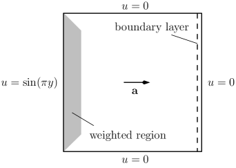
Figure 2: Schematics of the Eriksson-Johnson problem. Approximate location of the boundary layer shown as a dashed line and the weighted region is shaded.

Figure 3: Color map plots of $u$ in the Eriksson-Johnson problem with an analytic solution. Color range is uniformly set to $[0,1]$ and the minimum and maximum values of the solution are shown underneath each plot.

	$\epsilon=10^{-2}$	$\epsilon=10^{-4}$	$\epsilon=10^{-6}$
SN
	min/max = 0.00/0.84	min/max = 0.00/0.75	min/max = 0.00/0.75
WN
	min/max = 0.00/0.98	min/max = 0.00/0.95	min/max = 0.00/0.95
QON
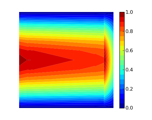
	min/max = 0.00/1.01	min/max = 0.00/0.99	min/max = 0.00/1.00
Reference

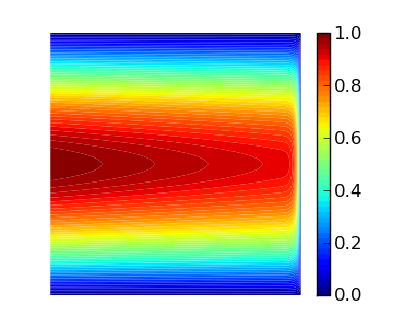
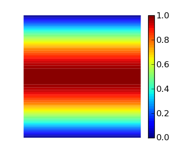
Advection Skew to the Mesh: Continuous Dirichlet Data

This problem has been studied in [16, 19] and consists of solving Equation (1) with the boundary conditions

$$u(0,y)=1-y,\quad u(x,0)=1-x,\quad u(x,1)=u(1,y)=0$$

and the advection vector $\mathbf{a}=(\cos\theta,\sin\theta)$, $\theta\in[0^{\circ},90^{\circ}]$. The solution features a boundary layer of width $\epsilon$ near the outflow boundary. We include a schematic of the problem in Figure 4 where the boundary layer is indicated by a dashed line and the weighted regions for the WN are shaded. For this problem, the reference solutions were computed using standard Galerkin FEM on a fine mesh which fully resolves the boundary layer. We were not able to compute such a solution for the problem with $\epsilon=10^{-6}$ although one can compare with the solution for $\epsilon=10^{-4}$ as the difference in this case is visually indistinguishable.

We observe similar performance of the SN and WN as compared to the previous problem (5). The QON in this case captures the main features of the solution well. However, while the WN exhibits a local overshoot in the solution for the $\epsilon=10^{-6}$ case, the solution value for the QON is underestimated across the domain. This occurs probably because the test functions are not sufficiently well resolved by our sub-grid discretization, see comments ahead.

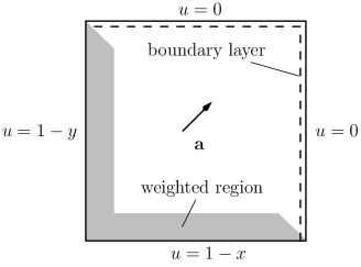
Figure 4: Schematics of the advection skew to the mesh problem with continuous Dirichlet data. Approximate location of the boundary layer shown as a dashed line and the weighted region is shaded.

Figure 5: Color map plots of $u$ in the advection skew to the mesh problem with continuous Dirichlet data. Color range is uniformly set to $[0,1]$ and the minimum and maximum values of the solution are shown underneath each plot.

	$\epsilon=10^{-2}$	$\epsilon=10^{-4}$	$\epsilon=10^{-6}$
SN
	min/max = 0.00/0.95	min/max = 0.00/0.90	min/max = 0.00/0.90
WN
	min/max = 0.00/1.12	min/max = 0.00/1.20	min/max = 0.0/1.20
QON
	min/max = 0.00/1.15	min/max = 0.01/0.95	min/max = 0.00/0.80
Reference			N/A

Advection Skew to the Mesh: Discontinuous Dirichlet Data

Our last problem is the standard benchmark test for the convection-diffusion equation in the engineering literature. The advection vector is the same as in the previous problem, but the inflow data is taken to be piecewise constant:

$$u(x,0)=1,\quad u(y,0)=\begin{cases}1,&0\leq y\leq 0.2\\ 0&0.2\leq y\leq 1\end{cases}$$

The problem schematic is shown in Figure 6 and the results in Figure 7. We emphasize here a feature of QON: if the mesh does not resolve the boundary layer, its effect is included but the layer is not resolved. This is in contrast to the SN and WN, where we always observe a boundary layer the width of one element. As in the previous problem, the reference solution has been obtained on a fine mesh using the standard Galerkin FEM.

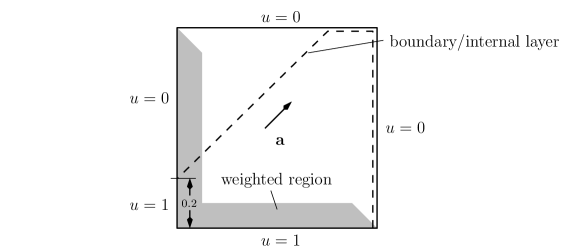
Figure 6: Schematics of the advection skew to the mesh problem with discontinuous Dirichlet data. Approximate location of the boundary layer shown as a dashed line and the weighted region is shaded.

Figure 7: Color map plots of $u$ in the advection skew to the mesh problem with discontinuous Dirichlet data. Color range is uniformly set to $[0,1]$ and the minimum and maximum values of the solution are shown underneath each plot.

	$\epsilon=10^{-2}$	$\epsilon=10^{-4}$	$\epsilon=10^{-6}$
SN
	min/max = -0.13/0.96	min/max = -0.14/0.91	min/max = -0.14/0.91
WN
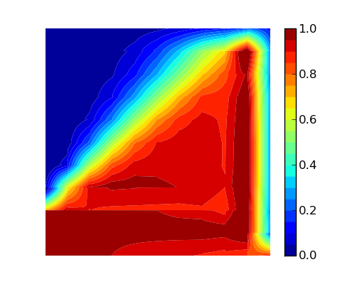
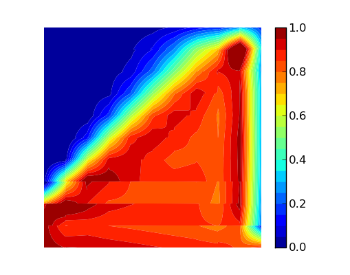
	min/max = -0.09/1.14	min/max = -0.10/1.26	min/max = -0.10/1.25
QON
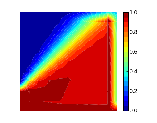
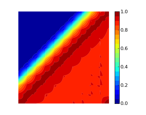
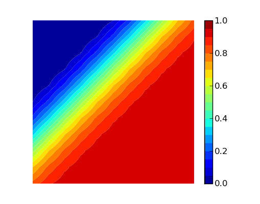
	min/max = -0.12/1.19	min/max = -0.04/1.04	min/max = -0.04/0.95
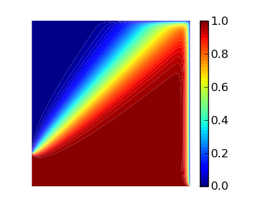
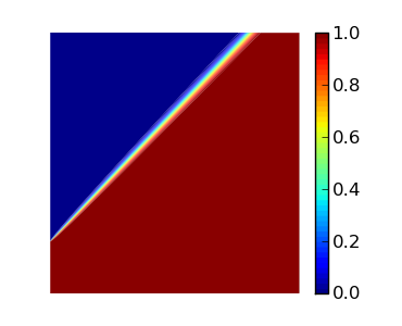
Reference			N/A

5.1 Norm Comparison: Mesh Refinement

We study the convergence of the different DPG schemes in the advection skew to the mesh problem with continuous Dirichlet data under uniform $h$ and $p$ refinements of the trial space. We compare the error of $u$ and $\boldsymbol{\sigma}$ with respect to the reference solution measured in the $L_{2}$ norm when $\epsilon=10^{-2}$. The purpose of this study is to show quantitatively the improved accuracy of the QON solution.

Results from this study are presented in Tables 1 and 2. Note that in each table, the reference solution comes from the standard Galerkin FEM with a fine mesh of rectangular bilinear elements. The values of $\boldsymbol{\sigma}_{\mathrm{ref}}$ were obtained by a linear interpolation of the coefficients determined from taking finite differences of the solution $u_{\mathrm{ref}}$. In both refinement strategies and for both $u$ and $\boldsymbol{\sigma}$, the QON provides better approximation to the reference solution, particularly when the mesh is coarse.

Table 1: Convergence of $u$ and $\boldsymbol{\sigma}$ under uniform $h$- and $p$-refinement in the advection skew to the mesh problem with continuous Dirichlet data at $\epsilon=10^{-2}$.

	$||u_{\mathrm{ref}}-u_{n}||_{L_{2}(\Omega)}$				$||\boldsymbol{\sigma}_{\mathrm{ref}}-\boldsymbol{\sigma}_{n}||_{L_{2}(\Omega)}$
$N$	SN	WN	QON		SN	WN	QON
5	2.55$\times 10^{-1}$	1.17$\times 10^{-1}$	7.69$\times 10^{-2}$		4.28$\times 10^{-2}$	4.15$\times 10^{-2}$	3.38$\times 10^{-2}$
10	1.76$\times 10^{-1}$	6.54$\times 10^{-2}$	4.84$\times 10^{-2}$		3.80$\times 10^{-2}$	3.68$\times 10^{-2}$	2.45$\times 10^{-2}$
25	6.26$\times 10^{-2}$	2.20$\times 10^{-2}$	1.43$\times 10^{-2}$		2.37$\times 10^{-2}$	2.33$\times 10^{-2}$	9.56$\times 10^{-3}$
50	1.64$\times 10^{-2}$	7.35$\times 10^{-3}$	4.33$\times 10^{-3}$		1.09$\times 10^{-2}$	1.08$\times 10^{-2}$	3.13$\times 10^{-3}$
100	3.24$\times 10^{-3}$	2.18$\times 10^{-3}$	1.17$\times 10^{-3}$		3.76$\times 10^{-3}$	3.74$\times 10^{-3}$	8.59$\times 10^{-4}$
	$||u_{\mathrm{ref}}-u_{n}||_{L_{2}(\Omega)}$				$||\boldsymbol{\sigma}_{\mathrm{ref}}-\boldsymbol{\sigma}_{n}||_{L_{2}(\Omega)}$
$p$	SN	WN	QON		SN	WN	QON
1	2.55$\times 10^{-1}$	1.17$\times 10^{-1}$	7.69$\times 10^{-2}$		4.28$\times 10^{-2}$	4.15$\times 10^{-2}$	3.38$\times 10^{-2}$
2	1.49$\times 10^{-1}$	5.56$\times 10^{-2}$	3.97$\times 10^{-2}$		3.45$\times 10^{-2}$	3.29$\times 10^{-2}$	2.36$\times 10^{-2}$
3	7.00$\times 10^{-2}$	2.72$\times 10^{-2}$	2.11$\times 10^{-2}$		2.37$\times 10^{-2}$	2.28$\times 10^{-2}$	1.43$\times 10^{-2}$
4	2.58$\times 10^{-2}$	1.30$\times 10^{-2}$	1.07$\times 10^{-2}$		1.40$\times 10^{-2}$	1.37$\times 10^{-2}$	7.66$\times 10^{-3}$

Table 2: Convergence of $u$ and $\boldsymbol{\sigma}$ under uniform $h$- and $p$-refinement in the advection skew to the mesh problem with continuous Dirichlet data at $\epsilon=10^{-4}$.

	$||u_{\mathrm{ref}}-u_{n}||_{L_{2}(\Omega)}$				$||\boldsymbol{\sigma}_{\mathrm{ref}}-\boldsymbol{\sigma}_{n}||_{L_{2}(\Omega)}$
$N$	SN	WN	QON		SN	WN	QON
5	3.73$\times 10^{-1}$	1.72$\times 10^{-1}$	7.05$\times 10^{-2}$		5.23$\times 10^{-3}$	5.23$\times 10^{-3}$	5.22$\times 10^{-3}$
10	3.60$\times 10^{-1}$	1.25$\times 10^{-1}$	6.50$\times 10^{-2}$		5.23$\times 10^{-3}$	5.22$\times 10^{-3}$	5.20$\times 10^{-3}$
25	3.51$\times 10^{-1}$	9.12$\times 10^{-2}$	6.61$\times 10^{-2}$		5.22$\times 10^{-3}$	5.21$\times 10^{-3}$	5.16$\times 10^{-3}$
50	3.45$\times 10^{-1}$	7.71$\times 10^{-2}$	6.46$\times 10^{-2}$		5.21$\times 10^{-3}$	5.18$\times 10^{-3}$	5.08$\times 10^{-3}$
100	3.36$\times 10^{-1}$	6.70$\times 10^{-2}$	6.15$\times 10^{-2}$		5.17$\times 10^{-3}$	5.13$\times 10^{-3}$	4.91$\times 10^{-3}$
	$||u_{\mathrm{ref}}-u_{n}||_{L_{2}(\Omega)}$				$||\boldsymbol{\sigma}_{\mathrm{ref}}-\boldsymbol{\sigma}_{n}||_{L_{2}(\Omega)}$
$p$	SN	WN	QON		SN	WN	QON
1	3.73$\times 10^{-1}$	1.72$\times 10^{-1}$	7.05$\times 10^{-2}$		5.23$\times 10^{-3}$	5.23$\times 10^{-3}$	5.22$\times 10^{-3}$
2	3.56$\times 10^{-1}$	1.24$\times 10^{-1}$	3.44$\times 10^{-2}$		5.23$\times 10^{-3}$	5.22$\times 10^{-3}$	5.20$\times 10^{-3}$
3	3.52$\times 10^{-1}$	1.00$\times 10^{-1}$	2.58$\times 10^{-2}$		5.22$\times 10^{-3}$	5.20$\times 10^{-3}$	5.17$\times 10^{-3}$
4	3.49$\times 10^{-1}$	9.16$\times 10^{-2}$	2.08$\times 10^{-2}$		5.20$\times 10^{-3}$	5.18$\times 10^{-3}$	5.13$\times 10^{-3}$

5.2 The Resolution of the Test Functions Corresponding to the Quasi-optimal Test Space Norm

The best approximation property of the DPG method hinges on the sufficient resolution of the optimal test functions. In the context of the quasi-optimal norm this is non-trivial because of the singular perturbation character of the auxiliary problem (21). While the subgrid discretization we have proposed is an effort to address this issue, the link between the accuracy of the test functions and the final solution is still unclear. This is partially due to the fact that the auxiliary problem is, to the best of our knowledge, unknown in the literature. Therefore, we make a numerical convergence assessment of the optimal test functions.

We restrict ourselves to $p$-refinements on the subgrid and measure the approximate relative error of the test functions in the quasi-optimal test space norm $|||\cdot|||_{\mathcal{W}(K)}$ as in

$$e(\tilde{p})=\frac{|||\mathbf{w}^{\tilde{p}+1}-\mathbf{w}^{\tilde{p}}|||_{\mathcal{W}(K)}}{|||\mathbf{w}^{\tilde{p}+1}|||_{\mathcal{W}(K)}}$$

This we carry out on a single square element $K$ of the ten by ten mesh used earlier in the advection skew to the mesh problems. Because the norm $|||\cdot|||_{\mathcal{W}(K)}$ is the usual energy norm for the auxiliary problems, its computation reduces to linear algebra. Recall that the columns of the matrix $\mathbf{U}_{\mathrm{opt}}$ represent the optimal test functions. Therefore the energy norm squared of the optimal test functions $\mathbf{w}_{i}$ is given by

$$|||\mathbf{w}_{i}|||^{2}_{\mathcal{W}(K)}=\mathbf{U}_{\mathrm{opt}}(:,i)^{T}\mathbf{K}_{\mathrm{opt}}\mathbf{U}_{\mathrm{opt}}(:,i)=\mathbf{U}_{\mathrm{opt}}(:,i)^{T}\mathbf{F}_{\mathrm{opt}}(:,i)=\mathbf{K}_{\ell}(i,i)$$

where we have adopted the MATLAB notation for indexing a whole row or column of a matrix. In other words, the energy norm of the optimal test functions may be read directly from the diagonal of $\mathbf{K}_{\ell}$.

Notice that when $p=1$, there are 28 trial functions and optimal test functions. To simplify the representation of the results, we separate the optimal test functions into four groups associated to the trial functions for $\boldsymbol{\sigma}$, $u$, $\hat{u}$, and $\hat{\sigma}_{n}$ and compute the average of the errors for each group. We present the results in Tables 3 and 4 for $\varepsilon=10^{-2}$ and $\varepsilon=10^{-4}$ where we have used $\bar{e}$ to indicate an average error and subscripts to refer to each group. We have also included the $L_{2}$ error with respect to the reference solution of $u$ in the table. The results show that while the optimal test functions corresponding to the field variables $\boldsymbol{\sigma}$ and $u$ are seemingly easy to approximate, those corresponding to the interface variables $\hat{\sigma}_{n}$ and $\hat{u}$ are problematic. As a matter of fact, the relative error level of the optimal test functions corresponding to the trace $\hat{u}$ barely decreases below the discretization error level for the field varible $u$ in the trial space as $\Delta p$ increases. This slow convergence explains the lull in the $h$-convergence in Table 2 as well as the degradation of the global accuracy when $\epsilon=10^{-6}$ in Figures 5 and 7. These phenomena are manifestations of the current practical limitations in the utilization of the quasi-optimal norm.

Table 3: Convergence of the optimal test functions in the advection skew to the mesh problems when $\epsilon=10^{-2}$, $N=10$ and $p=1$.

	average relative approximate errors
$\Delta p$	$\bar{e}_{\boldsymbol{\sigma}}$	$\bar{e}_{u}$	$\bar{e}_{\hat{u}}$	$\bar{e}_{\hat{\sigma}_{n}}$		$||u_{\mathrm{ref}}-u_{n}||_{L_{2}(\Omega)}$
1	2.16$\times 10^{-3}$	4.85$\times 10^{-3}$	9.42$\times 10^{-2}$	1.13$\times 10^{-3}$		4.62$\times 10^{-2}$
2	3.28$\times 10^{-4}$	7.38$\times 10^{-4}$	1.42$\times 10^{-2}$	1.67$\times 10^{-4}$		4.79$\times 10^{-2}$
3	3.08$\times 10^{-5}$	6.74$\times 10^{-5}$	1.77$\times 10^{-3}$	1.57$\times 10^{-5}$		4.84$\times 10^{-2}$
4	2.52$\times 10^{-6}$	5.34$\times 10^{-6}$	2.15$\times 10^{-4}$	1.30$\times 10^{-6}$		4.85$\times 10^{-2}$
5	4.22$\times 10^{-7}$	8.70$\times 10^{-7}$	4.23$\times 10^{-5}$	2.18$\times 10^{-7}$		4.85$\times 10^{-2}$
6	1.08$\times 10^{-7}$	2.20$\times 10^{-7}$	1.12$\times 10^{-5}$	5.58$\times 10^{-8}$		4.85$\times 10^{-2}$
7	3.44$\times 10^{-8}$	6.92$\times 10^{-8}$	3.59$\times 10^{-6}$	1.77$\times 10^{-8}$		4.85$\times 10^{-2}$
8	1.27$\times 10^{-8}$	2.53$\times 10^{-8}$	1.32$\times 10^{-6}$	6.54$\times 10^{-9}$		4.85$\times 10^{-2}$
9	5.22$\times 10^{-9}$	1.04$\times 10^{-8}$	5.45$\times 10^{-7}$	2.69$\times 10^{-9}$		4.85$\times 10^{-2}$

Table 4: Convergence of the optimal test functions in the advection skew to the mesh problems when $\epsilon=10^{-4}$, $N=10$ and $p=1$.

	average relative approximate errors
$\Delta p$	$\bar{e}_{\boldsymbol{\sigma}}$	$\bar{e}_{u}$	$\bar{e}_{\hat{u}}$	$\bar{e}_{\hat{\sigma}_{n}}$		$||u_{\mathrm{ref}}-u_{n}||_{L_{2}(\Omega)}$
1	2.07$\times 10^{-4}$	5.40$\times 10^{-3}$	4.54$\times 10^{-1}$	5.36$\times 10^{-3}$		9.15$\times 10^{-2}$
2	1.51$\times 10^{-5}$	3.00$\times 10^{-5}$	3.25$\times 10^{-1}$	7.65$\times 10^{-4}$		7.22$\times 10^{-2}$
3	8.17$\times 10^{-6}$	1.68$\times 10^{-5}$	1.48$\times 10^{-1}$	3.99$\times 10^{-4}$		6.50$\times 10^{-2}$
4	3.10$\times 10^{-6}$	6.22$\times 10^{-6}$	4.67$\times 10^{-2}$	1.50$\times 10^{-4}$		6.32$\times 10^{-2}$
5	1.17$\times 10^{-6}$	2.18$\times 10^{-6}$	1.43$\times 10^{-2}$	5.75$\times 10^{-5}$		6.29$\times 10^{-2}$
6	5.36$\times 10^{-7}$	9.49$\times 10^{-7}$	5.77$\times 10^{-3}$	2.67$\times 10^{-5}$		6.29$\times 10^{-2}$
7	2.97$\times 10^{-7}$	5.02$\times 10^{-7}$	3.56$\times 10^{-3}$	1.49$\times 10^{-5}$		6.29$\times 10^{-2}$
8	1.85$\times 10^{-7}$	3.09$\times 10^{-7}$	2.76$\times 10^{-3}$	9.24$\times 10^{-6}$		6.30$\times 10^{-2}$
9	1.24$\times 10^{-7}$	2.04$\times 10^{-7}$	2.39$\times 10^{-3}$	6.15$\times 10^{-6}$		6.31$\times 10^{-2}$

6 Concluding Remarks

We have studied the robustness of the discontinuous Petrov-Galerkin method with optimal test functions when applied to convection-diffusion problems. In particular, we have introduced a DPG scheme based on the quasi-optimal test norm and compared it with schemes based on other test space norms. Our numerical tests reveal that the quasi-optimal norm leads to improved coarse mesh accuracy as compared with the conventional DPG test space norms provided that the associated test functions are sufficiently well resolved. We have addressed the resolution of the optimal test functions by studying their convergence numerically. We have been able to find a compromise between accuracy and stability of the final DPG solution by combining a carefully designed element sub grid with numerical regularization of the test functions.

The DPG method with optimal test functions originates from the functional analytic foundation of the finite element method, and is perhaps still far from being adopted into engineering practice. We have made an attempt to popularize the methodology by contributing a holistic approach which begins in the abstract framework and ends in detailed explanation of the algorithm from the implementation viewpoint.

References

- [1] Babuška, I. Error-Bounds for Finite Element Method. Numerische Mathematik 16 (1971), 322–333.
- [2] Babuška, I., and Suri, M. On locking and robustness of the finite element method. SIAM Journal on Numerical Analysis 29 (1992), 1261–1293.
- [3] Barrett, J. W., and Morton, K. W. Approximate symmetrization and Petrov-Galerkin methods for diffusion-convection problems. Computer Methods in Applied Mechanics and Engineering 45 (1984), 97–122.
- [4] Bazilevs, Y., Calo, V. M., Cotrell, J. A., Evans, J. A., Lipton, S., Hughes, T. J. R., Scott, M. A., and Sederberg, T. W. Isogeometric analysis using T-splines. Computer Methods in Applied Mechanics and Engineering 199 (2010), 229–263.
- [5] Bottasso, C. L., Micheletti, S., and Sacco, R. The discontinuous Petrov-Galerkin method for elliptic problems. Computer Methods in Applied Mechanics and Engineering 191 (2002), 3391–3409.
- [6] Brezzi, F. On the existence, uniqueness and approximation of saddle-point problems arising from Lagrangian multipliers. RAIRO Analyse Numérique 8 (1974), 129–151.
- [7] Brezzi, F., Franca, L. P., Hughes, T. J. R., and Russo, A. . Computer Methods in Applied Mechanics and Engineering 145 (1997), 329–333.
- [8] Brezzi, F., Houston, P., Marini, D., and Süli, E. Modeling subgrid viscosity for advection–diffusion problems. Computer Methods in Applied Mechanics and Engineering 190, 13-14 (Dec. 2000), 1601–1610.
- [9] Brooks, A. N., and Hughes, T. J. R. Streamline upwind/Petrov-Galerkin formulations for convection dominated flows with particular emphasis on the incompressible Navier-Stokes equation. Computer Methods in Applied Mechanics and Engineering 32 (1982), 199–259.
- [10] Buffa, A., Hughes, T. J. R., and Sangalli, G. Analysis of a Multiscale Discontinuous Galerkin Method for Convection Diffusion Problems. SIAM Journal of Numerical Analysis 44 (2006), 1420–1440.
- [11] Codina, R. A finite element formulation for the numerical solution of the convection-diffusion equation. Tech. Rep. 14, International Center for Numerical Methods in Engineering (CIMNE), Barcelona, 1993.
- [12] Codina, R. Comparison of some finite element methods for solving the diffusion-convection-reaction equation. Computer Methods in Applied Mechanics and Engineering 156 (1998), 185–210.
- [13] Demkowicz, L. Babuška Brezzi. ICES REPORT 06-08, The Institute for Computational Engineering and Sciences, The University of Texas at Austin, 2006.
- [14] Demkowicz, L. Computing with hp-ADAPTIVE FINITE ELEMENTS: Volume 1 One and Two Dimensional Elliptic and Maxwell problems. CRC Press, United States of America, 2007.
- [15] Demkowicz, L., and Gopalakrishnan, J. A class of discontinuous Petrov-Galerkin methods. Part I: The transport equation. Computer Methods in Applied Mechanics and Engineering 199 (2009), 1558–1572.
- [16] Demkowicz, L., and Gopalakrishnan, J. A class of discontinuous Petrov-Galerkin methods. Part II: Optimal test functions. Numerical Methods for Partial Differential Equations 27 (2010), 70–105.
- [17] Demkowicz, L., and Gopalakrishnan, J. A New Paradigm for Discretizing Difficult Problems: Discontinuous Petrov-Galerkin Method with Optimal Test Functions. IACM Expressions 28 (2011), 12–19.
- [18] Demkowicz, L., and Gopalakrishnan, J. Analysis of the DPG Method for the Poisson Equation. SIAM Journal on Numerical Analysis 49, 5 (2011), 1788–1809.
- [19] Demkowicz, L., Gopalakrishnan, J., and Niemi, A. H. A class of discontinuous Petrov–Galerkin methods. Part III: Adaptivity. Applied Numerical Mathematics (Sept. 2011).
- [20] Demkowicz, L., and Heuer, N. Robust DPG method for convection-dominated diffusion problems. ICES REPORT 11-33, The Institute for Computational Engineering and Sciences, The University of Texas at Austin, 2011.
- [21] Demkowicz, L., and Oden, J. T. An adaptive characteristic Petrov-Galerkin finite element method for convection-dominated linear and nonlinear parabolic problems in one space variable. Journal of Computational Physics 67 (1986), 188–213.
- [22] Demkowicz, L., and Oden, J. T. An adaptive characteristic Petrov-Galerkin finite element method for convection-dominated linear and nonlinear parabolic problems in two space variables. Computer Methods in Applied Mechanics and Engineering 55 (1986), 63–87.
- [23] Eriksson, K., and Johnson, C. Adaptive Streamline Diffusion Finite Element Methods For Stationary Convection-Diffusion Problems. Mahtematics of Computation 60 (1993), 167–188.
- [24] Franca, L. P., Frey, S. L., and Hughes, T. J. R. Stabilized finite element methods. I. Application to the advective-diffusive model. Computer Methods in Applied Mechanics and Engineering 95 (1992), 253–276.
- [25] Franca, L. P., Hauke, G., and Masud, A. Revisiting stabilized finite element methods for the advective-diffusive equation. Computer Methods in Applied Mechanics and Engineering 195 (2006), 1560–1572.
- [26] Franca, L. P., Hughes, T. J. R., Loula, A. F. D., and Miranda, I. A New Family of Stable Elements for Nearly Incompressible Elasticity Based on a Mixed Petrov-Galerkin Finite Element Formulation. Numerische Mathematik 53 (1988), 123–141.
- [27] Guermond, J. Stabilization of Galerkin approximations of transport equations by subgrid modeling. Mathematical Modelling and Numerical Analysis 33, 6 (1999), 1293–1316.
- [28] Guermond, J. L. A Finite Element Technique for Solving First-Order PDEs in . SIAM Journal on Numerical Analysis 42, 2 (2004), 714–737.
- [29] Heinrich, J. C., Huyakorn, P. S., Zienkiewicz, O. C., and Mitchell, A. R. An ’upwind’ finite element scheme for two-dimensional convective transport equation. International Journal for Numerical Methods in Engineering 11 (1977), 131–143.
- [30] Hughes, T. J. R. The Finite Element Method: Linear Static and Dynamic Finite Element Analysis. Prentice-Hall, 1987.
- [31] Hughes, T. J. R., Cotrell, J. A., and Bazilevs, Y. Isogeometric analysis: CAD, finite elements, NURBS, exact geometry and meshrefinement. Computer Methods in Applied Mechanics and Engineering 194 (2005), 4135–4195.
- [32] Hughes, T. J. R., Evans, J. A., and Sangalli, G. Enforcement of Constraints and Maximum Principles in the Variational Multiscale Method. Computer Methods in Applied Mechanics and Engineering 199 (2009), 61–761.
- [33] Hughes, T. J. R., Scovazzi, G., and Franca, L. P. Multiscale and Stabilized Methods. In Encyclopedia of Computational Mechanics, Edited by Erwin Stein, René de Borst and Thomas J.R. Hughes. Volume 3: Fluids. John Wiley & Sons, 2007, pp. 59–137.
- [34] Jiang, B.-n. Non-oscillatory and Non-diffusive Solution of Convection Problems by the Iteratively Reweighted Least-Squares Finite Element Method. Journal of Computational Physics 105, 1 (Mar. 1993), 108–121.
- [35] Johnson, C. A new approach to algorithms for convection problems which are based on exact transport + projection. Computer Methods in Applied Mechanics and Engineering 100 (1992), 45–62.
- [36] Johnson, C., Nävert, U., and Pitkäranta, J. Finite element methods for linear hyperbolic problems. Computer Methods in Applied Mechanics and Engineering 45 (1984), 285–312.
- [37] Linß, T. Layer-adapted meshes for reaction-convection-diffusion problems. Lecture notes in mathematics. Springer, 2010.
- [38] Loula, A. F. D., Franca, L. P., Hughes, T. J. R., and Miranda, I. Stability, convergence and accuracy of new finite element method for the circular arch problem. Computer Methods in Applied Mechanics and Engineering 63 (1987), 281–303.
- [39] Loula, A. F. D., Hughes, T. J. R., and Franca, L. P. Petrov-Galerkin formulations of the Timoshenko beam problem. Computer Methods in Applied Mechanics and Engineering 63 (1987), 115–132.
- [40] Melenk, J. M., and Schwab, C. hp FEM for Reaction-Diffusion Equations I: Robust Exponential Convergence. SIAM Journal on Numerical Analysis 35, 4 (1998), 1520–1557.
- [41] Niemi, A. H., Bramwell, J. A., and Demkowicz, L. F. Discontinuous Petrov–Galerkin method with optimal test functions for thin-body problems in solid mechanics. Computer Methods in Applied Mechanics and Engineering 200, 9-12 (Feb. 2011), 1291–1300.
- [42] Niemi, A. H., Collier, N. O., and Calo, V. M. Discontinuous Petrov-Galerkin method based on the optimal test space norm for one-dimensional transport problems. Procedia Computer Science 4 (Jan. 2011), 1862–1869.
- [43] Niemi, A. H., Collier, N. O., and Calo, V. M. Discontinuous Petrov–Galerkin method based on the optimal test space norm for steady transport problems in one space dimension. Journal of Computational Science (Aug. 2011).
- [44] Oñate, E. Derivation of stabilized equations for numerical solution of advective-diffusive transport and fluid flow problems. Computer Methods in Applied Mechanics and Engineering 151 (1998), 233–265.
- [45] Schwab, C., and Suri, M. The p and hp versions of the finite element method for problems with boundary layers. Mathematics of Computation 65 (1996), 1403–1429.
- [46] Shishkin, G. I. Grid approximation of singularly perturbed boundary value problems with a regular boundary layer. Russian Journal of Numerical Analysis and Mathematical Modelling 4, 5 (1989), 397–418.
- [47] Xenophontos, C. The hp finite element method for singularly perturbed problems in smooth domains. Mathematical Models and Methods in Applied Sciences (M3AS) 8 (1998), 299–326.
- [48] Zitelli, J., Muga, I., Demkowicz, L., Gopalakrishnan, J., Pardo, D., and Calo, V. M. A class of discontinuous Petrov-Galerkin methods. Part IV: The optimal test norm and time-harmonic wave propagation in 1D. Journal of Computational Physics 230 (2011), 2406–2432.