MICROSTRUCTURE OF He II
IN THE PRESENCE OF BOUNDARIES

Abstract

We have studied the microstructure of a system of interacting Bose particles under zero boundary conditions and have found two possible orderings. One ordering is traditional and is characterized by the Bogolyubov dispersion law $E(k)\approx\sqrt{\left(\!\frac{\hbar^{2}k^{2}}{2m}\!\right)^{\!2}+qn\nu_{3}(k)\frac{\hbar^{2}k^{2}}{m}}$ ($q=1$) at a weak interaction. The second one is new and is characterized by the same dispersion law, but with $q=2^{-d}$, where $d$ is the number of noncyclic coordinates. At a weak interaction, the ground-state energy is less for the new solution. The boundaries affect the bulk microstructure due to the difference of the topologies of closed and open systems.

1 Introduction

In the Nature, all systems are finite, and the formulas deal with finite values. However, the explicit account for boundaries leads frequently to significant difficulties in the analysis. Therefore, the physicists use a special trick that allows one to avoid the consideration of boundaries, namely the passage to the thermodynamic limit (Т-limit): $N,V\rightarrow\infty$, $N/V={\rm const}$ [1]. This is the passage to infinite $N$ and $V$, rather than to very large ones: we increase infinitely the size of the system, the boundaries go to infinity and as if disappear. However, this reasoning contains a simple error: while the system is increasing, the boundaries cannot disappear, since they represent the topological property. By means of the continuous increase of a system with boundaries, it is impossible to obtain an infinite system without boundaries. The latter would occur at some topological jump, which we cannot imagine. This means that the passage to the T-limit assumes that such jump does not affect the bulk properties of the system. But it can affect in principle (no general proof of the opposite exists). To clarify the existence of such effect, it is necessary to study various systems. The goal of the present work is to study whether the boundaries affect the bulk microstructure of a Bose liquid and an interacting Bose gas.

In three models of interacting bosons [2,​ 3,​ 4,​ 5,​ 6], the solutions for a system with boundaries and a cyclic system are the same: for a homogeneous system at a weak interaction, they coincide with the Bogolyubov solution [7,​ 8]. In these models, the interatomic interaction was considered point-like (see Section 7 for details). But the interaction is not point-like in the Nature. We will find the solutions for a non-point interaction of the general form with a potential, which can be expanded in a Fourier series. It turns out that two solutions exist: traditional and new. We will study both solutions and compare them with the results of other models and with experiment.

2 Ground State of He II: Equations

Several methods of determination of the wave function (WF) $\Psi_{0}$ of the ground state (GS) of helium-II are available [8,​ 9,​ 10,​ 11,​ 12,​ 13,​ 14,​ 15,​ 16,​ 17,​ 18,​ 19,​ 20] (see also reviews [21,​ 22,​ 23]). In order not to take the boundaries into account, they used periodic boundary conditions (BCs) with passing to the T-limit. We will find the solutions for a system in a box with zero BCs. The influence of boundaries on the structure of the WF can be nontrivial. Therefore, it is expedient to use one of the exact analytic methods for the determination of $\Psi_{0}$ [10,​ 11,​ 12,​ 15], since the numerical methods may not catch the effect. We will operate within the method of collective variables [12,​ 24] used by us in [20,​ 25].

We transit to the collective variables

$$\rho_{\textbf{k}}=\frac{1}{\sqrt{N}}\sum\limits_{j=1}^{N}e^{-i\textbf{k}\textbf{r}_{j}}\quad(\textbf{k}\not=0),$$ (1)

where $N$ is the total number of atoms, and $\textbf{r}_{j}$ are the coordinates of atoms. For convenience, we introduce the following notation. The sums over the wave vectors

$$\textbf{k}=2\pi\left(\!\frac{j_{x}}{L_{x}},\frac{j_{y}}{L_{y}},\frac{j_{z}}{L_{z}}\!\right)\!,$$ (2)

where $j_{x},j_{y},j_{z}$ are integers, and $L_{x},L_{y},L_{z}$ are the sizes of the system, are denoted by the index $(2\pi)$: $\sum^{(2\pi)}$​; whereas the sums

$$\textbf{k}=\pi\left(\!\frac{j_{x}}{L_{x}},\frac{j_{y}}{L_{y}},\frac{j_{z}}{L_{z}}\!\right)$$ (3)

are denoted by the index $(\pi)$: $\sum^{(\pi)}$.

Under the periodic BCs with the subsequent passing to the T-limit, the solution for $\Psi_{0}$ was obtained by I. Yukhnovskii and I. Vakarchuk [12]:

$$\Psi_{0}=Ae^{S_{b}},$$ (4)

$$S_{b}=\sum\limits_{\textbf{k}_{1}\neq 0}^{(2\pi)}\frac{a_{2}(\textbf{k}_{1})}{2!}\rho_{\textbf{k}_{1}}\rho_{-\textbf{k}_{1}}+$$

$$+\sum\limits_{\textbf{k}_{1},\textbf{k}_{2}\neq 0}^{(2\pi)\textbf{k}_{1}+\textbf{k}_{2}\not=0}\frac{a_{3}(\textbf{k}_{1},\textbf{k}_{2})}{3!\sqrt{N}}\rho_{\textbf{k}_{1}}\rho_{\textbf{k}_{2}}\rho_{-\textbf{k}_{1}-\textbf{k}_{2}}+$$

$$+\!\sum\limits_{\textbf{k}_{1},\textbf{k}_{2},\textbf{k}_{3}\neq 0}^{(2\pi)\!\!\textbf{k}_{1}+\textbf{k}_{2}+\textbf{k}_{3}\not=0}\frac{a_{4}(\textbf{k}_{1},\textbf{k}_{2},\textbf{k}_{3})}{4!N}\rho_{\textbf{k}_{1}}\rho_{\textbf{k}_{2}}\rho_{\textbf{k}_{3}}\rho_{-\textbf{k}_{1}-\textbf{k}_{2}-\textbf{k}_{3}}+$$

$$+\,...,$$ (5)

where the functions $a_{j}(\textbf{k}_{1},...,\textbf{k}_{j-1})$ satisfy the chain of equations

$$E^{b}_{0}=\frac{N-1}{2N}n\nu_{3}(0)-\sum\limits_{\textbf{k}\not=0}^{(2\pi)}\frac{n\nu_{3}(k)}{2N}-\sum\limits_{\textbf{k}\not=0}^{(2\pi)}\frac{\hbar^{2}k^{2}}{2mN}a_{2}(\textbf{k}),$$ (6)

$$\frac{n\nu_{3}(k)m}{\hbar^{2}}+a_{2}(\textbf{k})k^{2}-a_{2}^{2}(\textbf{k})k^{2}=$$

$$=\sum\limits_{\textbf{q}\not=0}^{(2\pi)}\frac{a_{3}(\textbf{k},\textbf{q})}{N}(q^{2}+\textbf{k}\textbf{q})+\sum\limits_{\textbf{q}\not=0}^{(2\pi)}q^{2}\frac{a_{4}(\textbf{q},-\textbf{q},\textbf{k})}{2N},$$ (7)

$$a_{3}(\textbf{k},\textbf{q})\approx-2\frac{R(\textbf{k},\textbf{q})}{\epsilon_{0}(k)+\epsilon_{0}(q)+\epsilon_{0}(\textbf{k}+\textbf{q})},$$ (8)

$$R(\textbf{k},\textbf{q})=\textbf{k}\textbf{q}a_{2}(\textbf{k})a_{2}(\textbf{q})-\textbf{k}(\textbf{k}+\textbf{q})a_{2}(\textbf{k})a_{2}(\textbf{k}+\textbf{q})\,-$$

$$-\,\textbf{q}(\textbf{k}+\textbf{q})a_{2}(\textbf{q})a_{2}(\textbf{k}+\textbf{q}),$$ (9)

$$\epsilon_{0}(\textbf{k})=k^{2}(1-2a_{2}(\textbf{k})).$$ (10)

Here, $n=N/V$, $V$ is the volume of the system, $E_{0}^{b}$ is the ‘‘bulk’’ energy of the GS per atom, and

$$\nu_{3}(\textbf{k})\equiv\nu_{3}(k)=\int\limits_{-L_{x}}^{L_{x}}\!\!dx\int\limits_{-L_{y}}^{L_{y}}\!\!dy\int\limits_{-L_{z}}^{L_{z}}\!\!dzU_{3}(r)e^{-i\textbf{k}\textbf{r}}$$ (11)

is the Fourier-transform of the interaction potential $U_{3}(r)$ of two He⁴ atoms. The equation for $a_{3}$ is written in the zero approximation not involving the corrections $a_{4}$ and $a_{5}$, and the equations for higher corrections $a_{j\geq 4}(\textbf{k}_{1},...,\textbf{k}_{j-1})$ are not presented.

Consider He II in a rectangular vessel $L_{x}\times L_{y}\times L_{z}$ in size. The Hamiltonian has the form

$$\hat{H}=-\frac{\hbar^{2}}{2m}\sum\limits_{j}\triangle_{j}+\frac{1}{2}\sum\limits_{ij}^{i\not=j}U_{3}(|\textbf{r}_{i}-\textbf{r}_{j}|)+U_{2},$$ (12)

$$U_{2}=\sum\limits_{j}\left[U_{w}(x_{j})+U_{w}(L_{x}-x_{j})+U_{w}(y_{j})\,+\right.$$

$$+\left.U_{w}(L_{y}-y_{j})+U_{w}(z_{j})+U_{w}(L_{z}-z_{j})\right].$$ (13)

Here, $U_{2}$ is the interaction potential of helium atoms with all walls. The potentials of the walls are similar by form [26] to the interaction potential of two helium atoms. The free surface of liquid helium creates an energy barrier also, and we consider it as a wall. Below, we assume all barriers identical with the simple potential

$$U_{w}(x)=\left\{\!\!\begin{array}[]{lll}U_{s}>0,&\ x\leq 0,&\\[8.53581pt] 0,&\ x>0.&\end{array}\right.$$ (14)

We take $U_{s}$ finite, and the transition $U_{s}\rightarrow\infty$ will be made in final formulas.

Atoms polarize walls, and, therefore, the ‘‘reflections’’ of atoms arise on the walls. But since the potential of a wall is infinitely high, it absorbs the reflections, and we omit them in $\hat{H}$ (12).

Works [12,​ 24] used the non-Hermitian Bogolyubov–Zubarev Hamiltonian. Since the absence of the Hermitian property induces the questions [27], we will start from the ordinary Hermitian Hamiltonian (12).

Under zero BCs, the WF is nonzero inside the vessel and is equal to zero outside of it and on the boundary. Therefore, we seek the WF of helium atoms inside the vessel. In this case, all functions in the Schrödinger equation should be expanded in a Fourier series with regard for the fact that the coordinates $\textbf{r}_{j}$ of atoms are defined only inside the vessel. Let the system occupies a volume $x\in[0,L_{x}]$, $y\in[0,L_{y}]$, $y\in[0,L_{z}]$. The function $F(\textbf{r}_{1},\textbf{r}_{2})=\tilde{U}(|\textbf{r}_{1}-\textbf{r}_{2}|)$ can be expanded in a Fourier series in three ways: as a function of independent arguments $\textbf{r}_{1}$ and $\textbf{r}_{2}$, as a function of the argument $(\textbf{r}_{1}-\textbf{r}_{2})$ (modulus is considered as a part of the function), or as a function of $|\textbf{r}_{1}-\textbf{r}_{2}|$. In the first case,

$$\tilde{U}(|x_{1}-x_{2}|)\!=\!\frac{1}{L^{2}_{x}}\sum\limits_{k_{j_{1}}k_{j_{2}}}^{(2\pi)}\nu_{2}(k_{j_{1}},k_{j_{2}})e^{ik_{j_{1}}x_{1}+ik_{j_{2}}x_{2}},$$ (15)

$$\nu_{2}(k_{j_{1}},k_{j_{2}})\!=\!\int\limits_{0}^{L_{x}}dx_{1}\int\limits_{0}^{L_{x}}dx_{2}\tilde{U}(|x_{1}-x_{2}|)e^{-ik_{j_{1}}x_{1}-ik_{j_{2}}x_{2}}$$ (16)

(for simplicity, we restrict ourselves by the one-dimensional case). After some transformations, we obtain

$$\nu_{2}(k_{j_{1}},k_{j_{2}})=L_{x}\nu(k_{j_{1}})\delta_{k_{j_{1}},-k_{j_{2}}}+\tilde{\nu}_{2}(k_{j_{1}},k_{j_{2}}),$$ (17)

$$\nu(k_{j_{1}})=\int\limits_{-L_{x}}^{L_{x}}dx\tilde{U}(|x|)e^{-ik_{j_{1}}x}.$$ (18)

For a cyclic system, we have

$$\tilde{U}(|x_{1}-x_{2}|)\!=\!U(|x_{1}-x_{2}|)\!+\!U(L_{x}-|x_{1}-x_{2}|)$$ (19)

(on a ring, one atom acts on another one from two sides, which yields the ‘‘image’’ $U(L_{x}-|x_{1}-x_{2}|)$), and the nondiagonal part $\tilde{\nu}_{2}(k_{j_{1}},k_{j_{2}})$ is equal to zero. From whence (in 3D):

$$\tilde{U}_{3}(|\textbf{r}_{1}-\textbf{r}_{2}|)=\frac{1}{V}\sum\limits_{\textbf{k}}^{(2\pi)}\nu_{3}(\textbf{k})e^{i\textbf{k}(\textbf{r}_{1}-\textbf{r}_{2})}$$ (20)

with $\nu_{3}(\textbf{k})$ (11). Note that (11) contains the potential without images. At the transition to the T-limit, the images in $\tilde{U}_{3}$ are omitted. Then relations (11) and (20) set the standard Fourier-transformation for the T-limit.

For the system with boundaries, $\tilde{U}_{3}(|\textbf{r}_{1}-\textbf{r}_{2}|)=$ $=U_{3}(|\textbf{r}_{1}-\textbf{r}_{2}|)$ (no images) and $\tilde{\nu}_{2}(k_{j_{1}},k_{j_{2}})\neq 0$. However, formulas (11) and (20) are valid only for a potential with images, and their application to a potential without images distorts the initial potential: in the 1D case, series (20) gives potential (19) with image instead of the initial potential $U(|x_{1}-x_{2}|)$. This point is of importance, since the image $U(L_{x}-|x_{1}-x_{2}|)$ is unphysical for the system with boundaries, and its consideration causes the closure of the system by interaction.

When the nondiagonal part $\tilde{\nu}_{2}(k_{j_{1}},k_{j_{2}})\neq 0$ for the system with boundaries is considered, then the Fourier series (15), (17) reproduces the potential $U(|x_{1}-x_{2}|)$ exactly, without image. But the calculation of $\tilde{\nu}_{2}(k_{j_{1}},k_{j_{2}})$ is difficult. We can use a Fourier series, where the vector $(|x_{1}-x_{2}|,|y_{1}-y_{2}|,|z_{1}-z_{2}|)$ is the argument. But then the moduli will enter also in the exponent, and we cannot use the method of collective variables. Therefore, the best way is to use the expansion

$$U_{3}(|\textbf{r}_{1}-\textbf{r}_{2}|)=\frac{1}{2^{d}V}\sum\limits_{\textbf{k}}^{(\pi)}\nu_{3}(\textbf{k})e^{i\textbf{k}(\textbf{r}_{1}-\textbf{r}_{2})},$$ (21)

with $\nu_{3}(\textbf{k})$ (11). Here, the expansion argument is $(\textbf{r}_{1}-\textbf{r}_{2})$, and $x_{i}$ and $x_{j}$ take values from $[0,L_{x}]$, whereas $x_{i}-x_{j}\in[-L_{x},L_{x}].$ By the rules of Fourier analysis, the function $U_{3}(|\textbf{r}_{i}-\textbf{r}_{j}|)$ is expanded in series (11), (21): with k (3) and with the volume equal to $2L_{x}\times 2L_{y}\times 2L_{z}=2^{d}V$. This series is the simplest one, reproduces the initial potential exactly (without images, in particular), and is convenient for the method of collective variables. For the total interatomic potential, we obtain

$$\frac{1}{2}\sum\limits_{i\not=j}U_{3}(|\textbf{r}_{i}-\textbf{r}_{j}|)=\sum\limits_{\textbf{k}\not=0}^{(\pi)}\frac{n\nu_{3}(k)}{2^{d+1}}\rho_{\textbf{k}}\rho_{-\textbf{k}}\,+$$

$$+\,(N-1)\frac{n\nu_{3}(0)}{2^{d+1}}-\sum\limits_{\textbf{k}\not=0}^{(\pi)}\frac{n\nu_{3}(k)}{2^{d+1}}.$$ (22)

Under periodic BCs (in the T-limit or without it), we have [8]

$$\frac{1}{2}\sum\limits_{i\not=j}U_{3}(|\textbf{r}_{i}-\textbf{r}_{j}|)=\sum\limits_{\textbf{k}\not=0}^{(2\pi)}\frac{n\nu_{3}(k)}{2}\rho_{\textbf{k}}\rho_{-\textbf{k}}\,+$$

$$+\,(N-1)\frac{n\nu_{3}(0)}{2}-\sum\limits_{\textbf{k}\not=0}^{(2\pi)}\frac{n\nu_{3}(k)}{2}$$ (23)

(for a finite system, $U_{3}\rightarrow\tilde{U}_{3}$: we consider the images).

This is a key point. If the traditional expansion (11), (20), (23) is used, then we will obtain, obviously, the traditional solution for $E_{0}$ and $E(k)$ (with small ‘‘surface’’ corrections). But if expansion (11), (21), (23) is applied, we obtain, probably, a solution with $\nu_{3}(k)\rightarrow\nu_{3}(k)/2^{d}$ and $\sum^{(2\pi)}\rightarrow\sum^{(\pi)}$, since the bulk equations (5)–(8) are ‘‘generated’’ by the total potential. The solution cannot depend, of course, on the expansion. But some solution is better seen with the use of certain variables, whereas another one can be better seen in the language of other variables. Since the traditional solution was studied many times, we will consider a new solution following from expansion (11), (21).

Let us determine the ground state WF, which satisfies the Schrödinger equation

$$\hat{H}\Psi_{0}=NE_{0}\Psi_{0}$$ (24)

with Hamiltonian (12), (22). The main question is in which form we should seek $\Psi_{0}.$ Solution (4), (5) for periodic BCs is obtained from the requirement of the translation invariance and the functional independence [12] of the following collections of variables $\rho_{\textbf{k}}$:

$$\rho_{-\textbf{k}_{1}},\leavevmode\nobreak\ \rho_{-\textbf{k}_{1}}\rho_{-\textbf{k}_{2}},\leavevmode\nobreak\ \rho_{-\textbf{k}_{1}}\rho_{-\textbf{k}_{2}}\rho_{-\textbf{k}_{3}},\leavevmode\nobreak\ ...\,.$$ (25)

But the boundaries break the translation invariance. However, solution (4), (5) can be obtained without regard for the translation invariance, by substituting the bare function $\Psi_{0}=\rm const$, describing the free bosons, in the Schrödinger equation. The equation itself ‘‘sets’’ the form of corrections, which appear in the exponent. We will seek $\Psi_{0}$ analogously, by substituting the solution for free particles in the Schrödinger equation.

The WFs of the system of $N$ free Bose particles located in a rectangular box with potential (13), (14) are known. For identical states of all particles, the WFs are [28]

$$\Psi^{f}_{\textbf{l}}=\prod\limits_{j=1}^{N}\left[\sin{(k_{l_{x}}x_{j}+\delta_{l_{x}})}\sin{(k_{l_{y}}y_{j}+\delta_{l_{y}})}\right.\times$$

$$\times\left.\sin{(k_{l_{z}}z_{j}+\delta_{l_{z}})}\right],$$ (26)

where $l_{x},l_{y},l_{z}=1,2,3,...,$ and $k_{l_{x}}$ and $\delta_{l_{x}}$ satisfy the equations

$$\sin{\delta_{l_{x}}}=\frac{\gamma_{x}k_{l_{x}}L_{x}}{2},$$

$$\sin{(k_{l_{x}}L_{x}+\delta_{l_{x}})}=\pm\frac{\gamma_{x}k_{l_{x}}L_{x}}{2},$$ (27)

which yields

$$k_{l_{x}}L_{x}=\pi l_{x}-2\delta_{l_{x}},\quad\delta_{l_{x}}=\arcsin{(\gamma_{x}k_{l_{x}}L_{x}/2)}.$$ (28)

Here, we denote $\gamma_{x}=\frac{\hbar}{L_{x}}\sqrt{\frac{2}{mU_{s}}}$, and the values of $\arcsin$ are taken between $0$ and $\pi/2$. For the realistic systems, $\gamma_{x}\ll 1$. For example, for He⁴ atoms at $U_{s}=$ = 100 K and $L_{x}=10$ cm we have $\gamma_{x}\approx 4.92\times 10^{-10}$. At $l_{x}\ll 1/\pi\gamma_{x},$ relation (28) yields

$$k_{l_{x}}\approx l_{x}k_{1x}=l_{x}(1-\gamma_{x})\pi/L_{x},$$ (29)

$$\delta_{l_{x}}\approx l_{x}\delta_{1x}=l_{x}\pi\gamma_{x}/2.$$ (30)

The maximally possible values of $\delta_{l_{x}}$ and $k_{l_{x}}$ are determined from the condition $\sin{\delta_{l_{x}}}=1$:

$$\delta^{\rm max}_{l_{x}}=\pi/2,\quad k^{\rm max}_{l_{x}}=k_{1x}/\delta_{1x}.$$ (31)

The WF of the GS of a single atom inside of the box,

$$\Psi^{f}_{0,1}(\textbf{r})\!=\!\sin(k_{1x}x\!+\!\delta_{1x})\sin(k_{1y}y\!+\!\delta_{1y})\sin(k_{1z}z\!+\!\delta_{1z}),$$

is positive and nonzero. Outside of the box, the WF decays exponentially.

With regard for the above consideration, the WF of the ground state of $N$ interacting Bose particles located in the box can be sought in the form

$$\Psi_{0}=A_{1}\Psi^{f}_{\textbf{0}}e^{S_{w}^{(1)}+\tilde{S}_{b}},$$ (32)

where $\Psi^{f}_{\textbf{0}}$ is the WF of the GS of $N$ free Bose particles in the box (function (26) with $l_{x}=l_{y}=l_{z}=1$), $e^{\tilde{S}_{b}}$ is a WF of the form (4), (5) with the sums $\sum^{(\pi)}$ instead of $\sum^{(2\pi)}$ (this is seen from expansion (22)), and $e^{S_{w}^{(1)}}$ describes the cross terms arising at the substitution of $\Psi^{f}_{\textbf{0}}e^{\tilde{S}_{b}}$ in the Schrödinger equation. By the theorem on nodes, if the GS is nondegenerate, then $\Psi_{0}$ is nonzero in all points in the box. Therefore, it is convenient to lift the function $S_{w}^{(1)}$ to the exponent. The factor $e^{\tilde{S}_{b}}$ appears due to the interatomic interaction, and $\Psi^{f}_{\textbf{0}}$ ensures the fulfillment of BCs and the transition to the WF of free particles at the switch-off of the interaction.

Note that structure (32) was proposed previously by S. Yushchenko [29].

The function $\Psi_{0}$ (32) must satisfy the Schrödinger equation (24) and be zero at the boundaries. The last property is ensured at $U_{s}\rightarrow\infty$ by the factor $\Psi^{f}_{\textbf{0}}$ which satisfies the equations

$$-\frac{\hbar^{2}}{2m}\sum\limits_{j}\triangle_{j}\Psi^{f}_{\textbf{0}}+U_{2}\Psi^{f}_{\textbf{0}}=NE_{0}^{f}\Psi^{f}_{\textbf{0}},$$ (33)

$$E_{0}^{f}=\frac{\hbar^{2}k_{1}^{2}}{2m},\quad k_{1}^{2}=k_{1x}^{2}+k_{1y}^{2}+k_{1z}^{2}.$$ (34)

The function $\tilde{S}_{b}$ satisfies the equation

$$-\frac{\hbar^{2}}{2m}\sum\limits_{j}\triangle_{j}e^{\tilde{S}_{b}}+\frac{1}{2}\sum\limits_{i\not=j}U_{3}(|\textbf{r}_{i}-\textbf{r}_{j}|)e^{\tilde{S}_{b}}=N\tilde{E}^{b}_{0}e^{\tilde{S}_{b}}.$$ (35)

Then Eq. (24) is reduced to the equation for $S_{w}^{(1)}$:

$$-\frac{\hbar^{2}}{2m}\sum\limits_{j}\left[\triangle_{j}S_{w}^{(1)}+(\nabla_{j}S_{w}^{(1)})^{2}+2\nabla_{j}S_{w}^{(1)}\frac{\nabla_{j}\Psi^{f}_{\textbf{0}}}{\Psi^{f}_{\textbf{0}}}\,+\right.$$

$$+\left.2\nabla_{j}\tilde{S}_{b}\left(\!\nabla_{j}S_{w}^{(1)}+\frac{\nabla_{j}\Psi^{f}_{\textbf{0}}}{\Psi^{f}_{\textbf{0}}}\!\right)\right]=$$

$$=N(E_{0}-\tilde{E}_{0}^{b}-E_{0}^{f}),$$ (36)

$$\frac{\nabla_{j}\Psi^{f}_{\textbf{0}}}{\Psi^{f}_{\textbf{0}}}=\textbf{i}_{x}k_{1x}\cot{(k_{1x}x_{j}+\delta_{1x})}\,+$$

$$+\,\textbf{i}_{y}k_{1y}\cot(k_{1y}y_{j}\!+\!\delta_{1y})\!+\!\textbf{i}_{z}k_{1z}\cot(k_{1z}z_{j}\!+\!\delta_{1z}).$$ (37)

By seeking $\Psi_{0}$ inside of the vessel, we set $\cot{(k_{1x}x+\delta_{1x})}$ on the interval $[0,L_{x}]$. In order to apply the method of collective variables, we expand the cotangent in the Fourier series:

$$\cot{(k_{1x}x+\delta_{1x})}=\sum\limits_{j_{x}}^{(2\pi)}C_{1x}(j_{x})e^{i2\pi j_{x}x/L_{x}},$$ (38)

where $j_{x}$ runs all integers. We have

$$C_{1x}(j_{x})\!=\!-C_{1x}(-j_{x})\!=\!\int\limits_{0}^{L_{x}}\!\frac{dx}{L_{x}}\cot{(k_{1x}x\!+\!\delta_{1x})}e^{-iq_{x}x}=$$

$$=-2i\int\limits_{0}^{1/2}dx\sin{(2\pi j_{x}x)}\cot{(\pi x-2\delta_{1x}x+\delta_{1x})}.$$ (39)

From whence, $C_{1x}(0)=0$, and the function $C_{1x}(j_{x})$ is approximated by the formula

$$C_{1x}(j_{x}>0)\approx-i+\frac{i4j_{x}\delta_{1x}}{\pi}\ln\left(\!1+\frac{\pi}{4j_{x}\delta_{1x}}\!\right)\!,$$ (40)

which is valid at $j_{x}\ \lower-1.2pt\vbox{\hbox{\hbox to0.0pt{$<$\hss}\lower 5.0pt\vbox{\hbox{$\sim$}}}}\ j_{m}=1/\delta_{1x}$ with an error of $\leq 3\%$.

We note that $\cot{(k_{1x}x+\delta_{1x})}$ satisfies the requirements to functions expanded in the Fourier series. At $\delta_{1x}=0,$ we obtain $\cot{(\pi x/L_{x})}$, which does not satisfy these requirements, since $\int_{0}^{L_{x}}|\cot{(\pi x/L_{x})}|dx=$ $=\infty$. In view of this difficulty, we preserve all $\delta$ to be nonzero in calculations and set $\delta\rightarrow 0$ in final formulas.

Using the difference of the functional structure of the collections $\rho_{\textbf{k}}$ (25), we determine the structure of the solution for $S_{w}^{(1)}$ from (36)–(38) and (5):

$$S_{w}^{(1)}\!=\!\sum\limits_{\textbf{q}\neq 0}^{(2\pi)}S_{1}^{(1)}(\textbf{q})\rho_{-\textbf{q}}\!+\!\sum\limits_{\textbf{q},\textbf{q}_{1}\neq 0}^{\textbf{q}+\textbf{q}_{1}\neq 0}\!\frac{S_{2}^{(1)}(\textbf{q},\textbf{q}_{1})}{\sqrt{N}}\rho_{\textbf{q}_{1}}\rho_{-\textbf{q}_{1}-\textbf{q}}\,+$$

$$+\sum\limits_{\textbf{q},\textbf{q}_{1},\textbf{q}_{2}\neq 0}^{\textbf{q}+\textbf{q}_{1}+\textbf{q}_{2}\neq 0}\frac{S_{3}^{(1)}(\textbf{q},\textbf{q}_{1},\textbf{q}_{2})}{N}\rho_{\textbf{q}_{1}}\rho_{\textbf{q}_{2}}\rho_{-\textbf{q}_{1}-\textbf{q}_{2}-\textbf{q}}+...,$$ (41)

where q and $\textbf{q}_{j}$ run values (2) and (3), respectively (the first fact follows from (38), and the second does from (21), (49)). The functions $S_{j}^{(1)}$ satisfy the symmetry relations

$$S_{2}^{(1)}(\textbf{q},\textbf{q}_{1})=S_{2}^{(1)}(\textbf{q},-\textbf{q}-\textbf{q}_{1}),$$ (42)

$$S_{3}^{(1)}(\textbf{q},\textbf{q}_{1},\textbf{q}_{2})=S_{3}^{(1)}(\textbf{q},\textbf{q}_{2},\textbf{q}_{1})=$$

$$=S_{3}^{(1)}(\textbf{q},\textbf{q}_{1},-\textbf{q}-\textbf{q}_{1}-\textbf{q}_{2})=$$

$$=S_{3}^{(1)}(\textbf{q},-\textbf{q}-\textbf{q}_{1}-\textbf{q}_{2},\textbf{q}_{2}),$$ (43)

and the analogous ones can be written for higher $S_{j}^{(1)}$.

The equations for $S_{j}^{(1)}$ can be found from Eq. (36), if we substitute all functions in it and collect all terms referred to each collection in (25) and the constant. In view of the functional difference of collections in (25), we equate these groups of terms to zero. This yields the chain of equations for $E_{0}$ and the functions $S_{j}^{(1)}$:

$$E_{0}=\tilde{E}^{b}_{0}+A_{1},$$ (44)

$$A_{1}=\frac{\hbar^{2}}{2m}\left[k_{1}^{2}-\frac{1}{N}\sum\limits_{\textbf{q}\neq 0}^{(2\pi)}q^{2}S_{1}^{(1)}(\textbf{q})S_{1}^{(1)}(-\textbf{q})\,-\right.$$

$$\!-\!\left.\frac{i}{\sqrt{N}}\!\sum\limits_{q_{x}\neq 0}^{(2\pi)}\!2k_{1x}q_{x}C_{1x}(q_{x})S_{1}^{(1)}\!(-\textbf{q}_{x})\!+\!(x\!\rightarrow\!y,z)\!\right]\!,$$ (45)

$$S_{1}^{(1)}(\textbf{q})\epsilon_{0}(\textbf{q})=$$

$$=-i\sqrt{N}2k_{1x}q_{x}a_{2}(-\textbf{q}_{x})C_{1x}(q_{x})\delta_{\textbf{q},\textbf{q}_{x}}+(x\rightarrow y,z)\,+$$

$$+\frac{2}{N}\sum\limits_{\textbf{q}_{1}\neq 0}^{(\pi)}\left\{(q_{1}^{2}+\textbf{q}_{1}\textbf{q})S_{2}^{(1)}(\textbf{q},\textbf{q}_{1})\,+\right.$$

$$+\,3q_{1}^{2}S_{3}^{(1)}(\textbf{q},\textbf{q}_{1},-\textbf{q}_{1})\,+$$

$$+\,\sqrt{N}2q_{1}^{2}S_{1}^{(1)}(\textbf{q}_{1})S_{2}^{(1)}(\textbf{q}-\textbf{q}_{1},\textbf{q}_{1})\,+$$

$$+\left.0.5\sqrt{N}(q_{1}^{2}-\textbf{q}_{1}\textbf{q})S_{1}^{(1)}(\textbf{q}_{1})S_{1}^{(1)}(\textbf{q}-\textbf{q}_{1})\right\}+$$

$$+\Bigg{\{}\!\sum\limits_{p_{x}\neq 0}^{(2\pi)}2ik_{1x}C_{1x}(p_{x})\left[(q_{x}-p_{x})S_{1}^{(1)}(\textbf{q}-\textbf{p}_{x})\,-\right.$$

$$-\left.2p_{x}S_{2}^{(1)}(\textbf{q}-\textbf{p}_{x},-\textbf{q})\right]+(x\rightarrow y,z)\!\Bigg{\}}\!,$$ (46)

$$S_{2}^{(1)}(\textbf{q},\textbf{q}_{1})\left[\epsilon_{0}(\textbf{q}_{1})+\epsilon_{0}(\textbf{q}+\textbf{q}_{1})\right]+$$

$$+\,2S_{1}^{(1)}(\textbf{q})a_{2}(-\textbf{q}_{1})\textbf{q}\textbf{q}_{1}-q^{2}S_{1}^{(1)}(\textbf{q})a_{3}(\textbf{q},\textbf{q}_{1})=$$

$$=\delta_{\textbf{q},\textbf{q}_{x}}\sqrt{N}ik_{1x}C_{1x}(q_{x})\left\{2q_{1x}a_{2}(\textbf{q}_{1})\!-q_{x}a_{3}(\textbf{q}_{1},\textbf{q}_{x})\right\}+$$

$$+\sum\limits_{p_{x}\neq 0}^{(2\pi)}\!ik_{1x}C_{1x}(p_{x})\left[4(q_{x}\!+q_{1x}\!-p_{x})S_{2}^{(1)}(\textbf{q}\!-\textbf{p}_{x},\textbf{q}_{1})\,-\right.$$

$$-\left.6p_{x}S_{3}^{(1)}(\textbf{q}-\textbf{p}_{x},\textbf{q}_{1},-\textbf{q}-\textbf{q}_{1})\right]+(x\rightarrow y,z)\,+$$

$$+\frac{1}{\sqrt{N}}\sum\limits_{\textbf{q}_{2}\neq 0}^{(\pi)}\Bigg{\{}\!\frac{2}{\sqrt{N}}(q_{2}^{2}-\textbf{q}_{1}\textbf{q}_{2})S_{3}^{(1)}(\textbf{q},\textbf{q}_{1}-\textbf{q}_{2},\textbf{q}_{2})\,+$$

$$+\frac{4}{\sqrt{N}}\textbf{q}_{2}(\textbf{q}_{1}+\textbf{q}_{2}+\textbf{q})S_{3}^{(1)}(\textbf{q},\textbf{q}_{1},\textbf{q}_{2})\,-$$

$$-\,4\textbf{q}_{2}(\textbf{q}_{1}-\textbf{q}_{2}+\textbf{q})S_{1}^{(1)}(\textbf{q}_{2})S_{2}^{(1)}(\textbf{q}-\textbf{q}_{2},\textbf{q}_{1})\,+$$

$$+\,6q_{2}^{2}S_{1}^{(1)}(\textbf{q}_{2})S_{3}^{(1)}(\textbf{q}-\textbf{q}_{2},\textbf{q}_{1},-\textbf{q}-\textbf{q}_{1})\,+$$

$$+\,4(\textbf{q}_{1}+\textbf{q}_{2})^{2}S_{2}^{(1)}(\textbf{q}_{2},\textbf{q}_{1})S_{2}^{(1)}(\textbf{q}-\textbf{q}_{2},\textbf{q}_{1}+\textbf{q}_{2})\!\Bigg{\}}\!.$$ (47)

For brevity, we do not give the equations for the higher functions $S_{j\geq 3}^{(1)}(\textbf{q})$. Equation (47) should be symmetrized to satisfy (42). For the validity of relation (36), it is sufficient to consider only $S_{j}^{(1)}$ with the first even argument. We have the rule: the first argument of $S_{j}^{(1)}$ is quantized by the even law (2). Otherwise, we set $S_{j}^{(1)}=0$.

Analogously, (35) yields the chain of equations for $\tilde{E}^{b}_{0}$ and the functions $a_{j}$:

$$\tilde{E}^{b}_{0}=\frac{N-1}{2^{d+1}N}n\nu_{3}(0)-\sum\limits_{\textbf{k}\not=0}^{(\pi)}\frac{n\nu_{3}(k)}{2^{d+1}N}-\sum\limits_{\textbf{k}\not=0}^{(\pi)}\frac{\hbar^{2}k^{2}}{2mN}a_{2}(\textbf{k}),$$ (48)

$$\frac{n\nu_{3}(k)m}{2^{d}\hbar^{2}}+a_{2}(\textbf{k})k^{2}-a_{2}^{2}(\textbf{k})k^{2}=A_{2}(\textbf{k})\,+$$

$$+\sum\limits_{\textbf{q}\not=0}^{(\pi)}\frac{a_{3}(\textbf{k},\textbf{q})}{N}(q^{2}+\textbf{k}\textbf{q})+\sum\limits_{\textbf{q}\not=0}^{(\pi)}q^{2}\frac{a_{4}(\textbf{q},-\textbf{q},\textbf{k})}{2N},$$ (49)

$$a_{3}(\textbf{k},\textbf{q})\approx A_{3}(\textbf{k},\textbf{q})-\frac{2R(\textbf{k},\textbf{q})}{\epsilon_{0}(k)+\epsilon_{0}(q)+\epsilon_{0}(\textbf{k}+\textbf{q})}.$$ (50)

These equations can be found from (6)–(9) by the changes $\nu_{3}(k)\rightarrow\nu_{3}(k)/2^{d}$, $\sum\limits^{(2\pi)}\rightarrow\sum\limits^{(\pi)}$ and the addition of ‘‘surface’’ corrections $A_{j}$. The latter are related to the appearance of the terms

$$-\frac{\hbar^{2}}{2m}\sum\limits_{\textbf{k}\neq 0}^{(\pi)}A_{2}(\textbf{k})\rho_{\textbf{k}}\rho_{-\textbf{k}},$$

$$-\frac{\hbar^{2}}{2m}\sum\limits_{\textbf{k}_{1},\textbf{k}_{2}\neq 0}^{(\pi)\textbf{k}_{1}+\textbf{k}_{2}\neq 0}A_{3}(\textbf{k}_{1},\textbf{k}_{2})\rho_{\textbf{k}_{1}}\rho_{\textbf{k}_{2}}\rho_{-\textbf{k}_{1}-\textbf{k}_{2}},...$$

in Eq. (36), which have the structure of terms of Eq. (35). In particular,

$$A_{2}(\textbf{k})=\sum\limits_{q_{x}\neq 0}^{(2\pi)}\frac{ik_{1x}C_{1x}(-q_{x})}{\sqrt{N}}\left[4(q_{x}+k_{x})S_{2}^{(1)}(\textbf{q}_{x},\textbf{k})\,+\right.$$

$$+\left.6q_{x}S_{3}^{(1)}(\textbf{q}_{x},-\textbf{q}_{x},\textbf{k})\right]+(x\rightarrow y,z)\,+$$

$$+\frac{1}{N}\sum\limits_{\textbf{q}\neq 0}^{(2\pi)}\left[4(q^{2}+\textbf{q}\textbf{k})S_{1}^{(1)}(-\textbf{q})S_{2}^{(1)}(\textbf{q},\textbf{k})\,+\right.$$

$$+\,4(\textbf{k}+\textbf{q})^{2}S_{2}^{(1)}(\textbf{q},\textbf{k})S_{2}^{(1)}(-\textbf{q},-\textbf{k})\,+$$

$$+\left.6q^{2}S_{1}^{(1)}(-\textbf{q})S_{3}^{(1)}(\textbf{q},\textbf{k},-\textbf{k})\right]\!.$$ (51)

Though the majority of terms in (35) and (36) has the structure of the collections $\rho_{\textbf{k}}$, which is inherent only in the given equation ((35) or (36)), a small part of terms in (36) has the structure of terms in (35). The criterion for the construction of the chains of equations for $S_{j}^{(1)}$ and $a_{j}$ is the functional difference of the collections $\rho_{\textbf{k}}$ (25). Basically, the structures of the terms in (35) and (36) are different. Therefore, the partition of Eq. (24) into (35) and (36) is justified and simplifies the determination of $S_{w}^{(1)}$. The collections $\rho_{\textbf{k}}$, which are present in both equations, should be analyzed with the use of the initial equation (24). We can verify that $\Psi_{0}$ (32) satisfies Eq. (24), if $a_{j}$ and $A_{j}$ satisfy Eqs. (48)–(51).

As $U_{s}\rightarrow\infty$ and $\delta\rightarrow 0,$ relations (32), (41), (44)–(51) are the required solution for the WF of the ground state of $N$ interacting Bose particles filling a rectangular vessel.

The analysis of Eqs. (46) and (47) indicates that the functions $S_{1}^{(1)}(\textbf{q})$ and $S_{2}^{(1)}(\textbf{q},\textbf{q}_{1})$ can be considered ‘‘one-dimensional’’:

$$S_{1}^{(1)}(\textbf{q})\!\approx\!\delta_{\textbf{q},\textbf{q}_{x}}S_{1}^{(1)}(\textbf{q}_{x})+\delta_{\textbf{q},\textbf{q}_{y}}S_{1}^{(1)}(\textbf{q}_{y})+\delta_{\textbf{q},\textbf{q}_{z}}S_{1}^{(1)}(\textbf{q}_{z}),$$ (52)

$$S_{2}^{(1)}(\textbf{q},\textbf{q}_{1})\approx\delta_{\textbf{q},\textbf{q}_{x}}S_{2}^{(1)}(\textbf{q}_{x},\textbf{q}_{1})\,+$$

$$+\,\delta_{\textbf{q},\textbf{q}_{y}}S_{2}^{(1)}(\textbf{q}_{y},\textbf{q}_{1})+\delta_{\textbf{q},\textbf{q}_{z}}S_{2}^{(1)}(\textbf{q}_{z},\textbf{q}_{1})$$ (53)

($\textbf{q}\equiv(q_{x},q_{y},q_{z})=\textbf{q}_{x}+\textbf{q}_{y}+\textbf{q}_{z}$), since the nonone-dimensional $S_{j}^{(1)}$ with $\textbf{q}=(q_{x},q_{y},0)$ (with possible permutations of the $x$-, $y$-, and $z$-components) and $\textbf{q}=(q_{x},q_{y},q_{z})$ are less than one-dimensional ones by, respectively, $N^{1/3}$ and $N^{2/3}$ times. Due to the smallness of nonone-dimensional terms, their inclusion in the equations does not influence the values of one-dimensional ones and the value of $E_{0}$. For the one-dimensional parts of the functions $S_{j}^{(1)},$ all terms in Eqs. (46) and (47) are of the same order, as it is easy to verify. Therefore, all they should be taken into account. But, in this case, (44)–(47) is a complicated system of nonlinear integral equations difficult to be solved. Below, we will use the simplest zero approximations for $S_{1}^{(1)}$ and $S_{2}^{(1)}$:

$$S_{1}^{(1)}(\textbf{q}_{x})\approx-\frac{i\sqrt{N}k_{1x}C_{1x}(q_{x})2a_{2}(-\textbf{q}_{x})}{q_{x}-2q_{x}a_{2}(\textbf{q}_{x})},$$ (54)

$$S_{2}^{(1)}(\textbf{q}_{x},\textbf{q}_{1})\approx$$

$$\approx\frac{i\sqrt{N}k_{1x}C_{1x}(q_{x})}{1-2a_{2}(\textbf{q}_{x})}\frac{2q_{1x}a_{2}(\textbf{q}_{1})-q_{x}a_{3}(\textbf{q}_{1},\textbf{q}_{x})}{\epsilon_{0}(\textbf{q}_{1})+\epsilon_{0}(\textbf{q}_{x}+\textbf{q}_{1})}.$$ (55)

It is easy to verify that the surface corrections $A_{1}$ and $A_{2}$ have no effect on the solutions for $E_{0}$ and $a_{2}(k)$. We expect that $A_{j\geq 3}$ do not affect the solutions for $a_{j\geq 3}$. However, the boundaries change the ‘‘bulk part’’ of the equations for $E_{0}$ and $a_{j}$: the network of vectors k becomes by a factor of $2^{d}$ denser, and the Fourier-transform of the potential is multiplied by $1/2^{d}$. For this reason, the boundaries strongly influence the values of $E_{0}$ and $a_{j}$.

Besides WF (32), WFs of the form (32) with $\Psi^{f}_{\textbf{0}}\rightarrow$ $\rightarrow\Psi^{f}_{\textbf{l}}$ (and $\textbf{k}_{1}\rightarrow\textbf{k}_{\textbf{l}}$) are also the solutions. But such WFs are equal to zero at many points inside the vessel.

3 Ground State of He II: Solutions

The sines standing before the exponential function in $\Psi_{0}$ (32) set an inhomogeneous arc-like distribution of atoms in the vessel. For this reason, the anxieties arose [30,​ 31,​ 32] that the use of bare sines will not allow one to construct the series of perturbation theory so that a reasonable behavior of the density (the constant density of He II in the whole volume except for a narrow strip near the wall) be obtained. Apparently, namely for this reason, the problem was solved with periodic BCs, rather than with zero BCs; and the above-obtained solution was lost. Therefore, it is important to verify solution (32) in this aspect. Let us find the behavior of the density. Since the function $e^{\tilde{S}_{b}}$ sets a homogeneous distribution of atoms, we need to consider the behavior of the ansatz $\Psi^{f}_{\textbf{0}}e^{S_{w}^{(1)}}$ in (32). The function $S_{w}^{(1)}(\textbf{r}_{1},...,\textbf{r}_{N})$ (41) contains the one-particle dependence in each sum, and the values are of the same order. But taking the sums with $S_{j\geq 2}^{(1)}$ into account is a complicated task, and we neglect it. Then

$$\Psi_{0}(x_{1})\sim f(\textbf{r}_{1})=\sin{(k_{1x}x_{1}+\delta_{1x})}e^{s_{1}(\textbf{r}_{1})},$$ (56)

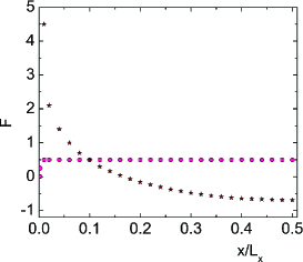
Fig. 1.: Values of the functions $f(x)$ ($\circ$) and $s_{1}(x)$ ($\star$) by formulas (56), (58) for potentials (14) and (59) at $a=2\,\mbox{\AA}$, $U_{b}=1600\,$K, $U_{bd}=0\,$K, $U_{s}\rightarrow\infty,$ and the vessel size $L_{x}=10^{4}\bar{R}$. Values of $f(x)$ and $s_{1}(x)$ at $x/L_{x}\in[0.5,1]$ are obtained by the reflection of the curves in an upright mirror positioned at $x=0.5L_{x}$

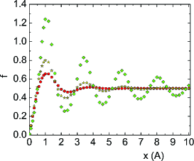
Fig. 2.: Values of the function $f(x)$ (56), (58) near the wall ($x=0$) at $L_{x}=10^{4}\bar{R}$, $U_{s}\rightarrow\infty,$ and potential (59) with $a=2\,\mbox{\AA}$, $b=4\,\mbox{\AA}$, $U_{bd}=-9\,$K, and three barriers: $U_{b}=800\,$K ($\circ$), $U_{b}=2000\,$K ($\star$), and $U_{b}=2900\,$K ($\diamond$). At $x\ \lower-1.2pt\vbox{\hbox{\hbox to0.0pt{$>$\hss}\lower 5.0pt\vbox{\hbox{$\sim$}}}}\ 6\,\mbox{\AA},$ curves $\circ\circ\circ$ and $\star\star\star$ almost merge. Values of $x$ are given in Å

$$s_{1}(\textbf{r}_{1})=\sum\limits_{q_{x}\neq 0}^{(2\pi)}\frac{S_{1}^{(1)}(\textbf{q}_{x})}{\sqrt{N}}e^{iq_{x}x_{1}}\,+$$

$$+\sum\limits_{q_{x},q_{y}\neq 0}^{(2\pi)}\frac{S_{1}^{(1)}(\textbf{q}_{x}+\textbf{q}_{y})}{\sqrt{N}}e^{iq_{x}x_{1}+iq_{y}y_{1}}\,+$$

$$+\sum\limits_{q_{x},q_{z}\neq 0}^{(2\pi)}\frac{S_{1}^{(1)}(\textbf{q}_{x}+\textbf{q}_{z})}{\sqrt{N}}e^{iq_{x}x_{1}+iq_{z}z_{1}}\,+$$

$$+\!\!\!\sum\limits_{q_{x},q_{y},q_{z}\neq 0}^{(2\pi)}\!\!\frac{S_{1}^{(1)}(\textbf{q}_{x}+\textbf{q}_{y}+\textbf{q}_{z})}{\sqrt{N}}e^{iq_{x}x_{1}+iq_{y}y_{1}+iq_{z}z_{1}}.$$ (57)

As was noted in Sec. 2, we have $S_{1}^{(1)}(\textbf{q}_{x}+\textbf{q}_{y}+\textbf{q}_{z})\sim$ $\sim S_{1}^{(1)}(\textbf{q}_{x}+\textbf{q}_{y})/N^{1/3}\sim S_{1}^{(1)}(\textbf{q}_{x})/N^{2/3}.$ Therefore, three last sums in (57) are of the order of the first one, but they depend additionally on $y_{1}$ and $z_{1}$. Let us consider only the first sum:

$$s_{1}(\textbf{r}_{1})=s_{1}(x_{1})=\sum\limits_{q_{x}=2\pi j_{x}/L_{x}}^{(2\pi)}\frac{S_{1}^{(1)}(\textbf{q}_{x})}{\sqrt{N}}e^{iq_{x}x_{1}},$$ (58)

where $j_{x}=\pm 1,\pm 2,\pm 3,...\,$. For $S_{1}^{(1)}(\textbf{q}_{x}),$ we use the zero approximation (54). In view of the property $S_{1}^{(1)}(-\textbf{q}_{x})=S_{1}^{(1)}(\textbf{q}_{x})$ and since $S_{1}^{(1)}(\textbf{q}_{x})$ is real, the imaginary part of (58) is cancelled, and we can change $e^{iq_{x}x_{1}}\rightarrow\cos{(q_{x}x_{1})}$. In this paper, we study only the qualitative behavior of the solutions. Therefore, we choose the interatomic potential of two He⁴ atoms in the simple form

$$U_{3}(\textbf{r})\approx\left\{\!\!\begin{array}[]{ll}U_{b}>0,&\ r\leq a,\\[2.84526pt] U_{bd}<0,&\ a\leq r\leq b,\\[2.84526pt] 0,&\ r>b.\end{array}\right.$$ (59)

For the modern potentials [33,​ 34], $a\approx 2.6\,\mbox{\AA}$, $U_{bd}\approx$$\approx-11\,$K, but the barrier and the well are more flat than steps (59). Therefore, we will use the lower values of $a$ and $|U_{bd}|$ in (59): $a=2\,\mbox{\AA}$, $U_{bd}=-9\,$K, and $b=4\,\mbox{\AA}$.

The Fourier-transform (11) of potential (59) is

$$\nu_{3}(k)=\frac{4\pi}{k^{3}}\left\{[U_{b}-U_{bd}][\sin{(ak)}-ak\cos{(ak)]}\right.+$$

$$+\left.U_{bd}[\sin{(bk)}-bk\cos{(bk)}]\right\}\!.$$ (60)

In the two-particle approximation, we have from (49):

$$a_{2}(k)=\frac{1}{2}-\sqrt{\frac{1}{4}+\frac{n\nu_{3}(k)m}{2^{d}\hbar^{2}k^{2}}}.$$ (61)

We chose the sign ‘‘minus’’ before the root in Eq. (61). At the sign ‘‘plus,’’ we have nonphysical result $E_{0}=-\infty$.

The results for the functions $f(x_{1})$ and $s_{1}(x_{1})$ (56), (58) at $L_{x}=10^{4}\bar{R}$ and several potentials are given in Figs. 1 and 2; here, $\bar{R}\approx 3.58\,\mbox{\AA}$ is the mean interatomic distance for He II. The values of the functions at $L_{x}=10^{5}\bar{R}$ and $L_{x}=10^{3}\bar{R}$ differ from the drawn ones very slightly (by $\ \lower-1.2pt\vbox{\hbox{\hbox to0.0pt{$<$\hss}\lower 5.0pt\vbox{\hbox{$\sim$}}}}\ 0.1\%$). So, the curves in the figures are true for all $L_{x}\ \lower-1.2pt\vbox{\hbox{\hbox to0.0pt{$>$\hss}\lower 5.0pt\vbox{\hbox{$\sim$}}}}\ 10^{3}\bar{R}$. As seen from Fig. 1, $f(x_{1})$ is equal to 0.5 everywhere, except for a narrow region near the wall. While approaching the wall, $f(x_{1})$ oscillates with constant period and increasing amplitude and becomes zero on the wall. An increase of the interatomic barrier $U_{b}$ causes a growth of the amplitude of oscillations $f(x_{1})$. The well depth $U_{bd}$ does not affect the results, if $|U_{bd}|\ll U_{b}$. As the distance to the wall increases, $f(x_{1})$ approaches the constant $0.5$ with a high accuracy increasing with $L_{x}$. For example, at $L_{x}=10^{4}\bar{R},$ the deviation from 0.5 occurs only in the sixth decimal point. As $x_{1}\rightarrow L_{x},$ the function $f(x_{1})$ behaves itself as at $x_{1}\rightarrow 0$.

It is of interest that $f(x_{1})$ oscillates near the wall. This is due to the short-range order, and the period is proportional to $a/\bar{R}$. Large oscillations at $U_{b}=$ $=2900\,$K are, most likely, nonphysical and are related to the neglect of corrections, which are large at such a potential. This reflects the behavior of the density $\rho$ of helium, since $\rho(x_{1})\sim\int dy_{1}dz_{1}d\textbf{r}_{2}...d\textbf{r}_{N}|\Psi_{0}|^{2}\sim$ $\sim f^{2}(x_{1})$ (the behavior of $\rho(x_{1})$ near the wall is also affected by $e^{\tilde{S}_{b}}$, but we did not study it).  Similar oscillations were obtained in [16], while modeling the properties of a film of helium adsorbed on the substrate.

We obtained the solutions also at finite $U_{s}$. At $U_{s}\ \lower-1.2pt\vbox{\hbox{\hbox to0.0pt{$>$\hss}\lower 5.0pt\vbox{\hbox{$\sim$}}}}\ 1000\,$K, they are practically invariable with increase in $U_{s}$, except for the values on a wall, where $f\neq 0$. As $U_{s}$ increases, $s_{1}(x)$ approaches a constant ($\simeq 10$) at $x=0$, and $\sin{(k_{1x}x+\delta_{1x})}\rightarrow 0.$ As a result, we have $f(x\rightarrow 0)|_{U_{s}\rightarrow\infty}\rightarrow 0$. With regard for the higher corrections, such behavior will be conserved: as $U_{s}\rightarrow\infty,$ we have $\delta\rightarrow 0,$ such $\delta$ affects slightly $C_{1}(q)$ and all results, because $\delta$ enters the equations through the function $C_{1}(q)$. In addition, the terms with large $q$ are cut in sums by $a_{j}.$ Due to such properties, the transition $U_{s}\rightarrow\infty$, $\delta\rightarrow 0$ is correct and makes $\Psi_{0}$ to be arbitrarily close to zero on the walls.

Thus, though the bare function $\sin{(k_{1x}x+\delta_{1x})}$ is far from to be a constant, the account for $S_{1}^{(1)}(q_{x})$ makes the theoretical density of atoms to be constant everywhere, except for a narrow ($\sim$Å) region near walls. Sines are the best bare functions, because 1) their use gives the simplest equations; 2) if the interatomic interaction is ‘‘switched-off,’’ $\Psi_{0}$ is reduced to the product of bare sines, which is the ground-state WF of $N$ free Bose particles in the box. The circumstance that the correction $S_{1}^{(1)}(q_{x})$ ‘‘improves’’ the behavior of $f(x_{1})$ seems natural, because the Schrödinger equation (24) involves the interaction of atoms and must make their distribution uniform, but $S_{1}^{(1)}(q_{x})$ is generated just by the Schrödinger equation.

4 Excited State of He II

We now find the WF of helium II in a vessel for the state with one phonon. Under periodic BCs, the exact solution for the WF takes the form [24]

$$\Psi_{\textbf{k}}(\textbf{r}_{1},...,\textbf{r}_{N})=\psi_{\textbf{k}}\Psi_{0},$$ (62)

$$\psi_{\textbf{k}}\equiv\psi^{b}_{\textbf{k}}=\rho_{-\textbf{k}}+\sum\limits_{\textbf{k}_{2}\neq 0,-\textbf{k}}^{(2\pi)}\frac{b_{2}(\textbf{k}_{2},\textbf{k})}{\sqrt{N}}\rho_{\textbf{k}_{2}}\rho_{-\textbf{k}_{2}-\textbf{k}}\,+$$

$$+\sum\limits_{\textbf{k}_{2},\textbf{k}_{3}\neq 0}^{(2\pi)\,\textbf{k}_{2}+\textbf{k}_{3}+\textbf{k}\not=0}\frac{b_{3}(\textbf{k}_{2},\textbf{k}_{3},\textbf{k})}{N}\rho_{\textbf{k}_{2}}\rho_{\textbf{k}_{3}}\rho_{-\textbf{k}_{2}-\textbf{k}_{3}-\textbf{k}}+...\,.\vspace*{-11mm}$$ (63)

A solution in the zero approximation

$$\psi^{b}_{\textbf{k}}=\rho_{-\textbf{k}}$$ (64)

with a simplified first correction with $b_{2}$ was first proposed by R. Feynman [35,​ 36]. The arguments in favor of solution (62), (63) are as follows: 1) it satisfies the Schrödinger equation for $N$ interacting Bose particles and 2) it is an eigenfunction of the momentum operator $\hat{\textbf{P}}=-i\hbar\sum_{j}\nabla_{\textbf{r}_{j}}$ with the eigenvalue $\hbar\textbf{k}$; 3) at the ‘‘switching-off’’ of the interaction, it is reduced to WF (64) describing $N$ free Bose particles, from which $N-1$ particles are immovable, and the single one moves with the momentum k; 4) an analogous solution is obtained in the operator approach [8]; 5) the completeness [12] of collections (25) implies that the solution for $\psi_{\textbf{k}}$ should have only such a form. However, the structure of (62) is the assumption, though no solution with another structure was found. The solution for $\psi_{\textbf{k}}$ with ‘‘shadow’’ variables [17,​ 18] is equivalent to (62), (63).

The simplest way to find solution (62), (63) is to assume the structure of (62) and to substitute the WF of free particles (64), as the bare $\psi_{\textbf{k}}$, in the Schrödinger equation for interacting particles. The equation prompts the form of corrections to $\psi_{\textbf{k}}$.

In a similar manner, we start for the liquid in a vessel from (62) with $\Psi_{0}$ (32). The study of different possibilities has shown that $\psi_{\textbf{k}}$ must be sought in the form

$$\psi_{\textbf{k}_{\textbf{r}}}=\frac{8}{\sqrt{N}}\sum\limits_{j=1}^{N}\cos{(k_{r_{x}}x_{j})}\cos{(k_{r_{y}}y_{j})}\cos{(k_{r_{z}}z_{j})}\,+$$

$$+\,\delta\psi_{\textbf{k}_{\textbf{r}}}=\rho_{-\textbf{k}_{\textbf{r}}}+7\,\mbox{permutations}+\delta\psi_{\textbf{k}_{\textbf{r}}}$$ (65)

with the unknown $\delta\psi_{\textbf{k}_{\textbf{r}}}.$ The permutation means $\rho_{-\textbf{k}_{\textbf{r}}}$ with the different sign of one or several components of $\textbf{k}_{\textbf{r}}$. In this case, $\textbf{k}_{\textbf{r}}$ takes values (3), since we must obtain the solution for free particles at the switching-off of the interaction. We now represent $\psi_{\textbf{k}}$ in the form

$$\psi_{\textbf{k}}=\psi^{0}_{\textbf{k}}+7\,\mbox{permutations},$$ (66)

$$\psi^{0}_{\textbf{k}}=\rho_{-\textbf{k}}+\delta\psi^{0}_{\textbf{k}}.$$ (67)

Solution (66), (67) describes a 3D standing wave decaying into eight counterrunning waves.

Substituting WF (62) in the Schrödinger equation with Hamiltonian (12), we obtain the equa- tions for $\psi_{\textbf{k}}$:

$$-\frac{\hbar^{2}}{2m}\sum\limits_{j}\left\{\triangle_{j}\psi_{\textbf{k}}+2(\nabla_{j}\psi_{\textbf{k}})\times\nabla_{j}S\right\}=E(\textbf{k})\psi_{\textbf{k}},$$ (68)

$$S=S^{(1)}_{w}+\tilde{S}_{b}+S_{0},$$ (69)

$$S_{0}=\ln{\Psi^{f}_{\textbf{0}}},$$ (70)

where $E(\textbf{k})=E-NE_{0}$ is the energy of a quasiparticle; $E(\textbf{k})$ is obviously independent of the signs of components of $\textbf{k}.$ Therefore, Eq. (68) is separated into 8 equations: for $\psi^{0}_{\textbf{k}}$ and 7 permutations with the same energy $E(k)$.

The analysis indicates that the solution for $\psi^{0}_{\textbf{k}}$ has the following form:

$$\psi^{0}_{\textbf{k}}=\psi^{b}_{\textbf{k}}+b_{0}(\textbf{k})+\sum\limits_{\textbf{q}\neq 0,-\textbf{k}}^{(2\pi)}Q_{1}(\textbf{q},\textbf{k})\rho_{-\textbf{q}-\textbf{k}}\,+$$

$$+\sum\limits_{\textbf{q},\textbf{q}_{1}\neq 0}^{\textbf{q}+\textbf{q}_{1}+\textbf{k}\not=0}\frac{Q_{2}(\textbf{q},\textbf{q}_{1},\textbf{k})}{\sqrt{N}}\rho_{\textbf{q}_{1}}\rho_{-\textbf{q}-\textbf{q}_{1}-\textbf{k}}\,+$$

$$+\sum\limits_{\textbf{q},\textbf{q}_{1},\textbf{q}_{2}\neq 0}^{\textbf{q}+\textbf{q}_{1}+\textbf{q}_{2}+\textbf{k}\not=0}\frac{Q_{3}(\textbf{q},\textbf{q}_{1},\textbf{q}_{2},\textbf{k})}{N}\rho_{\textbf{q}_{1}}\rho_{\textbf{q}_{2}}\rho_{-\textbf{q}-\textbf{q}_{1}-\textbf{q}_{2}-\textbf{k}}\,+$$

$$+...,$$ (71)

where $\psi^{b}_{\textbf{k}}$ is of the form of solution (63) for periodic BCs (but with $\textbf{k}_{j}$ running series (3)), $b_{0}$ and $Q_{l}$ are the corrections from boundaries. Here, q is quantized according to (2) (like $2\pi j/L$), and $\textbf{q}_{j}$ and k are quantized by (3) (like $\pi j/L$).

With regard for the properties of $\rho_{\textbf{k}}$, we can directly verify that $\Psi_{\textbf{k}}$ (62), (66), (71) is the exact solution of the Schrödinger equation, if the functions $E(k)$, $b_{j},$ and $Q_{l}$ satisfy the equations

$$b_{0}(\textbf{k})\epsilon(k)=-2k^{2}S_{1}^{(1)}(-\textbf{k})\delta_{\textbf{k},\textbf{k}^{e}}\,-$$

$$-\,2k_{1x}k_{x}iC_{1x}(-k_{x})\sqrt{N}\delta_{\textbf{k},\textbf{k}_{x}^{e}}\,-$$

$$-\,\frac{2}{\sqrt{N}}\sum\limits_{\textbf{q}\neq 0}^{(\pi)}q^{2}Q_{2}(-\textbf{k},\textbf{q},\textbf{k})\delta_{\textbf{k},\textbf{k}^{e}}\,-$$

$$-\sum\limits_{\textbf{q}\neq 0,-\textbf{k}}^{(2\pi)}2(\textbf{k}+\textbf{q})^{2}Q_{1}(\textbf{q},\textbf{k})S_{1}^{(1)}(-\textbf{k}-\textbf{q})\delta_{\textbf{k},\textbf{k}^{e}}\,+$$

$$+\sum\limits_{q_{x}\neq 0}^{(2\pi)}2\sqrt{N}k_{1x}q_{x}iC_{1x}(q_{x})Q_{1}(-\textbf{k}-\textbf{q}_{x},\textbf{k})\delta_{\textbf{k},\textbf{k}^{e}}\,+$$

$$+\,(x\rightarrow y,z),$$ (72)

$$\epsilon(k)=\epsilon_{0}(k)-\frac{1}{N}\sum\limits_{\textbf{k}_{2}\neq 0}^{(\pi)}b_{2}(\textbf{k}_{2},\textbf{k})2\textbf{k}_{2}(\textbf{k}_{2}+\textbf{k})\,-$$

$$-\frac{1}{N}\sum\limits_{\textbf{k}_{2}\neq 0}^{(\pi)}6k^{2}_{2}b_{3}(\textbf{k}_{2},-\textbf{k}_{2},\textbf{k})\,-$$

$$-\sum\limits_{q_{x}\neq 0}^{(2\pi)}2k_{1x}(k_{x}+q_{x})iC_{1x}(-q_{x})Q_{1}(\textbf{q}_{x},\textbf{k})\,-$$

$$-\frac{2}{\sqrt{N}}\sum\limits_{\textbf{q}\neq 0}^{(2\pi)}Q_{1}(\textbf{q},\textbf{k})(\textbf{k}+\textbf{q})\,\times$$

$$\times\left[\textbf{q}S_{1}^{(1)}(-\textbf{q})+2(\textbf{k}+\textbf{q})S^{(1)}_{2}(-\textbf{q},-\textbf{k})\right]+$$

$$+\sum\limits_{q_{x}\neq 0}^{(2\pi)}4k_{1x}q_{x}iC_{1x}(q_{x})Q_{2}(-\textbf{q}_{x},\textbf{q}_{x},\textbf{k})\,-$$

$$-\frac{4}{\sqrt{N}}\sum\limits_{\textbf{q}\neq 0}^{(2\pi)}q^{2}Q_{2}(-\textbf{q},\textbf{q},\textbf{k})S_{1}^{(1)}(\textbf{q})+(x\rightarrow y,z),$$ (73)

$$Q_{1}(\textbf{q},\textbf{k})\left[\epsilon(k)-\epsilon_{0}(\textbf{k}+\textbf{q})\right]=$$

$$=\,2ik_{1x}C_{1x}(q_{x})\delta_{\textbf{q},\textbf{q}_{x}}\left[-k_{x}+2q_{x}b_{2}(\textbf{q},\textbf{k})\right]+$$

$$+\frac{2S_{1}^{(1)}(\textbf{q})}{\sqrt{N}}[\textbf{q}\textbf{k}-2q^{2}b_{2}(\textbf{q},\textbf{k})]-\frac{4k^{2}}{\sqrt{N}}S_{2}^{({1})}(\textbf{q},-\textbf{q}-\textbf{k})\,-$$

$$-\frac{1}{N}\sum\limits_{\textbf{q}_{1}\neq 0}^{(\pi)}\left\{2\textbf{q}_{1}(\textbf{q}_{1}+\textbf{q}+\textbf{k})\right.\times$$

$$\times\,[Q_{2}(\textbf{q},\textbf{q}_{1},\textbf{k})+Q_{1}(\textbf{q}+\textbf{q}_{1},\textbf{k})\sqrt{N}S_{1}^{(1)}(-\textbf{q}_{1})]\,+$$

$$+\,6q_{1}^{2}Q_{3}(\textbf{q},\textbf{q}_{1},-\textbf{q}_{1},\textbf{k})\,+$$

$$+\,4q_{1}^{2}Q_{2}(\textbf{q}-\textbf{q}_{1},\textbf{q}_{1},\textbf{k})\sqrt{N}S_{1}^{(1)}(\textbf{q}_{1})+Q_{1}(\textbf{q}+\textbf{q}_{1},\textbf{k})\,\times$$

$$\times\left.4(\textbf{q}_{1}+\textbf{q}+\textbf{k})^{2}\sqrt{N}S_{2}^{(1)}(-\textbf{q}_{1},-\textbf{q}-\textbf{k})\!\right\}+$$

$$+\!\!\sum\limits_{p_{x}\neq 0}^{(2\pi)}2k_{1x}iC_{1x}(p_{x})\left[(-k_{x}-q_{x}+p_{x})Q_{1}(\textbf{q}-\textbf{p}_{x},\textbf{k})\right.+$$

$$+\left.2p_{x}Q_{2}(\textbf{q}-\textbf{p}_{x},\textbf{p}_{x},\textbf{k})\right]+(x\rightarrow y,z),$$ (74)

$$b_{2}(\textbf{k}_{2},\textbf{k})\left[\epsilon(k)-\epsilon_{0}(\textbf{k}_{2})-\epsilon_{0}(\textbf{k}+\textbf{k}_{2})\right]=$$

$$=\textbf{k}\textbf{k}_{2}a_{2}(\textbf{k}_{2})-\textbf{k}(\textbf{k}+\textbf{k}_{2})a_{2}(\textbf{k}+\textbf{k}_{2})-k^{2}a_{3}(\textbf{k},\textbf{k}_{2})\,-$$

$$-\frac{2}{\sqrt{N}}\sum\limits_{\textbf{k}_{3}\neq 0}^{(\pi)}\bigg{\{}\!\frac{3\textbf{k}_{3}(\textbf{k}_{2}+\textbf{k}_{3}+\textbf{k})}{\sqrt{N}}b_{3}(\textbf{k}_{2},\textbf{k}_{3},\textbf{k})\,+$$

$$+\,Q_{1}(\textbf{k}_{3},\textbf{k})(\textbf{k}_{3}+\textbf{k})\left[2(\textbf{k}_{3}-\textbf{k}_{2})S_{2}^{(1)}(-\textbf{k}_{3},\textbf{k}_{2})\right.+$$

$$+\left.3(\textbf{k}_{3}+\textbf{k})S_{3}^{(1)}(-\textbf{k}_{3},\textbf{k}_{2},-\textbf{k}_{2}-\textbf{k})\right]+$$

$$+\,2Q_{2}(-\textbf{k}_{3},\textbf{k}_{2}+\textbf{k}_{3},\textbf{k})(\textbf{k}_{2}+\textbf{k}_{3})\,\times$$

$$\times\left[\textbf{k}_{3}S_{1}^{(1)}(\textbf{k}_{3})+2(\textbf{k}_{2}+\textbf{k}_{3})S_{2}^{(1)}(\textbf{k}_{3},\textbf{k}_{2})\right]+$$

$$+\,3k_{3}^{2}S_{1}^{(1)}(\textbf{k}_{3})Q_{3}(-\textbf{k}_{3},\textbf{k}_{2},-\textbf{k}_{2}-\textbf{k},\textbf{k})\!\bigg{\}}\,+$$

$$+\sum\limits_{p_{x}\neq 0}^{(2\pi)}2k_{1x}iC_{1x}(p_{x})\left[3p_{x}Q_{3}(-\textbf{p}_{x},\textbf{k}_{2},-\textbf{k}_{2}-\textbf{k},\textbf{k})\right.+$$

$$+\left.2(k_{2x}+p_{x})Q_{2}(-\textbf{p}_{x},\textbf{k}_{2}+\textbf{p}_{x},\textbf{k})\right]+$$

$$+\,\mbox{higher corrections}+(x\rightarrow y,z),$$ (75)

where $\epsilon(k)=2mE(k)/\hbar^{2}$, $\textbf{k}^{e}$ is the wave vector with even components (i.e., they are multiple to $2\pi/L$), $\textbf{q}_{x}=q_{x}\textbf{i}_{x},\textbf{q}_{y}=q_{y}\textbf{i}_{y},\textbf{q}_{z}=q_{z}\textbf{i}_{z},$ and analogously for $\textbf{p}_{x}$, $\textbf{p}_{y}$, and $\textbf{p}_{z}.$ By $(x\rightarrow y,z),$ we denote the same terms as that with the separated $x$-component, but with the changes $x\rightarrow y$ and $x\rightarrow z$.

Equations (72)–(75) are written in the approximation of ‘‘two sums in the wave vector’’, at which the series contain the functions $a_{2}$, $a_{3}$, $b_{2}$, $b_{3}$, $S^{(1)}_{j\leq 3}$, and $Q_{l\leq 3}$ and do not include the corrections $a_{j\geq 4}$, $b_{j\geq 4}$, $S^{(1)}_{j\geq 4},$ and $Q_{l\geq 4}$ (they change the equation for $b_{2}$, by adding the correcting sums with $b_{4}$, $S^{(1)}_{4},$ and $Q_{4}$).

If the interaction is switched-off, $\Psi_{\textbf{k}}$ reveals a complicated structure, which should be reduced to the solution for free particles; but we omit this point.

Let us consider the properties of Eqs. (71)–(75). Solution (63) was obtained under periodic BCs and contains only the functions $b_{j\geq 2}$. Solution (71) corresponds to the zero BCs and contains the additional functions $b_{0}$ and $Q_{l}$. In view of the ‘‘one-dimensional’’ form (52), (53) of the functions $S_{j}^{(1)}$, relations (72)–(75) imply that the functions $Q_{l}$ can be also considered ‘‘one-dimensional.’’ In particular,

$$Q_{1}(\textbf{q},\textbf{k})\approx Q_{1}(\textbf{q}_{x},\textbf{k})\delta_{\textbf{q},\textbf{q}_{x}}\,+$$

$$+\,Q_{1}(\textbf{q}_{y},\textbf{k})\delta_{\textbf{q},\textbf{q}_{y}}+Q_{1}(\textbf{q}_{z},\textbf{k})\delta_{\textbf{q},\textbf{q}_{z}}.$$ (76)

The ‘‘two-dimensional’’ $Q_{1}$ with q of the form $(q_{x},q_{y},0)$ and the ‘‘three-dimensional’’ ones with $\textbf{q}=$ $=(q_{x},q_{y},q_{z})$ are less than the one-dimensional ones by $\sim$$N^{1/3}$ and $\sim$$N^{2/3}$ times, respectively. Due to the smallness of ‘‘non-1D’’ $Q_{1},$ their inclusion in the equations does not affect the values of one-dimensional ones. The estimates indicate that $Q_{l}$ affects $\epsilon(k)$ negligibly. In Eq. (75), the surface corrections for $b_{2}$ are also less than the bulk ones by $\sim$$N^{1/3}$ times. The smallness of surface corrections $A_{l}$ and $Q_{l}$ is related to the thinness of a near-surface fluid layer as compared with the sizes of a system.

Therefore, we set $Q_{l}=0$ in Eqs. (71)–(75). Then we obtain the Vakarchuk–Yukhnovskii equations [24] for $\epsilon(k)$ and $b_{j}$. However, $\textbf{k}_{j}$ in these equations should be quantized by the $\pi/L$-law (3) instead of the usually used $2\pi/L$-law (2), which is valid for the periodic BCs. In the zero approximation for $\Psi_{0}$ and $\Psi_{\textbf{k}},$ we set $a_{j\geq 3}=0$ and $b_{j}=0$ in the equations. Then we obtain the formula for the energy of quasiparticles:

$$E(k)\approx\sqrt{\left(\frac{\hbar^{2}k^{2}}{2m}\right)^{2}+\frac{n\nu_{3}(k)}{2^{d}}\frac{\hbar^{2}k^{2}}{m}},$$ (77)

which is close to the Bogolyubov one, but it contains the additional factor $1/2^{d}$ due to the boundaries (in the general case, $d$ is the number of nonperiodic coordinates). This formula is true at a weak interaction. Comparing formula (77) at potential (59) with the dispersion curve of He II as $k\rightarrow 0$, we obtain $U_{b}\simeq 283\,$K, whereas we have $U_{b}\simeq 35\,$K without the factor $1/2^{d}$. The first estimate is more plausible.

The Bogolyubov–Zubarev model [8] gives the same results, if we expand the potential in the Fourier series (21): in [8], we replace $\nu_{3}(k)\rightarrow\nu_{3}(k)/2^{d}$, $\sum^{(2\pi)}\rightarrow\sum^{(\pi)}$ and obtain $E(k)$ (77) and $E_{0}$ (48) with $a_{2}(k)$ (61).

Relations $\partial\langle\hat{H}\rangle/\partial\nu_{3}(k)=\langle\partial\hat{H}/\partial\nu_{3}(k)\rangle$, $S(k)=$ $=\langle\rho_{\textbf{k}}\rho_{-\textbf{k}}\rangle$ and (22) yield [24] $S(k)=1+(2^{d+1}/n)\,\times$ $\times\,(\partial E_{0}/\partial\nu_{3}(k))$. Using this result, (44), and (48), we find the connection between $a_{2}(k)$ and the structural factor $S(k)$. In the zero approximation, this connection is the same as for periodic BCs: $1-2a_{2}(k)\approx$ $\approx 1/S(k)$. With regard for this relation and (61), formula (77) is transformed into the Feynman formula

$$E(k)\approx\frac{\hbar^{2}k^{2}}{2mS(k)},$$ (78)

which agrees approximately with the experiment.

If one particle is in the box, $k$ is restricted from above by the value $k^{\rm max}=\sqrt{6mU_{s}}/\hbar$ (see (31)). For ${\rm He}^{4}$ atoms at $U_{s}=25\,K$, we have $k^{\rm max}\approx 3.6\,\mbox{\AA}^{-1}$. So, the observed break of the dispersion curve of He II at $k\approx 3.6\,\mbox{\AA}^{-1}$ can be caused, in principle, by that a phonon has also some $k^{\rm max}$ at a finite $U_{s}$, rather than by the decay mechanism [37].

5 Comparison
of the New and Traditional Solutions

Expansion (11), (20) yields the traditional solution. For the transition to it, it is necessary to replace $1/2^{d}\rightarrow 1$, $\sum^{(\pi)}\rightarrow\sum^{(2\pi)}$ in the equations. The curves in Figs. 1 and 2 are true also for the traditional solution, but for $U_{b}$ which is less by a factor of 8. For a cyclic system, we have only this traditional solution. But, for a system with boundaries, we obtain the traditional and new solutions.

The principal question is as follows: Which of the solutions is realized in the Nature for systems with boundaries? We found numerically that, at a weak interaction, $E_{0}$ is noticeably less for the new solution (usually by $\sim 2^{d}$ times): in 2D and 3D cases for all parameters, and in 1D case almost for all ones. We studied potentials (59) and $U_{b}\delta(x/a)$ for 1D and potential (59) for 2D. For 3D, we took (59) and

$$U_{3}(\textbf{r})\approx\left\{\!\!\begin{array}[]{ll}\displaystyle U_{b}(1-r^{2}/a^{2}),&r\leq a,\\[2.84526pt] \displaystyle U_{bd}\left[\!\left(\!1-\frac{a}{r_{0}}\!\right)^{\!\!2}-\left(\!\frac{r}{r_{0}}-1\!\right)^{\!\!2}\!\right]\!,&\ a\leq r\leq\tilde{b},\\[5.69054pt] 0,&\ r>\tilde{b},\end{array}\right.$$ (79)

where $\tilde{b}=2r_{0}-a$. The quantity $E_{0}$ was calculated by formulas (48) and (61). In 2D, potential (59) has the Fourier-transform

$$\nu_{2}(\textbf{k})=\frac{2\pi a}{k}(U_{b}-U_{bd})J_{1}(ka)+\frac{2\pi b}{k}U_{bd}J_{1}(kb).$$ (80)

Here, $J_{1}(p)$ is the Bessel function. We consider the weakness of the interaction as the smallness of the barrier $U_{b}$ and (for 3D) of the concentration $n$. At a nonweak interaction, $E_{0}$ for the new solution is sometimes less than that for the traditional one. But the opposite is also possible; this depends on the approximation, the parameters and, possibly, the error of calculations.

The solution with larger $E_{0}$ corresponds to the unstable ordering. Therefore, the new solution is true at a weak interaction; but we don’t know which solution is true at a strong interaction. As was mentioned above, the traditional solution for the systems with boundaries follows from expansion (11), (20), which creates $2^{d}-1$ fictitious images and makes the total interatomic potential cyclic. In such system, there is no symmetry breaking that corresponds to the boundary, besides the hand-imposed condition $\Psi=0$. Such statement of the problem is not quite self-consistent, since we are interested in the topological effect, but the topology is modeled unproperly. This calls into question the traditional solution. However, this solution was found [38] also from the exact expansion (11), (21) in the Gross–Pitaevskii approach. Therefore, the traditional solution can also exist in our approach.

6 Why Can the Boundaries
Affect the Bulk Properties?

To argue why the boundaries should not affect the bulk properties, the following general arguments are presented: 1) for large systems, the volume of the near-boundary region is negligibly small as compared with the total volume of the system; 2) the dimensional formulas of the form $E=Nf(S/N,V/N)$ [39]; 3) the proofs [40] of the existence of a thermodynamic limit. These are not simple questions, and they are slightly studied. We will try now to clarify them. First, the above-obtained effect of boundaries has the bulk character (see below); in this case, argument (1) is not valid. We now answer item (3), which will also answer item (2). It was proved in monograph [40] that if, for a cyclic system or a system with boundaries, $N$ and $V$ are unboundedly increased at $N/V=$ const, then the partition function approaches some limiting value. If we perform the same transition in the above-obtained formulas for a cyclic or noncyclic system, then the equations remain invariant, i.e., the limits exist too. Therefore, our results agree with those in [40]. However, such limit is almost obvious [40] without calculations. The following is not obvious: Do the limits for initially cyclic and initially noncyclic systems coincide? This was not considered in [40]. In our approach, these limits turn out different. Another question is as follows: Do the limits [40] mean the transition to the infinite system? The passage to limit was performed by Van Hove and by Fisher. In both cases, the finite system was considered, and the passage to infinity is realized in the meaning of the continuous limit $N,V\rightarrow\infty$. For a cyclic system, we can continuously pass to the infinite system, whereas it is impossible for a system with boundaries: a boundaries cannot disappear at increasing the system size, because the boundary is a topological property (this can be referred to a lot of remarkable paradoxes for infinite sets [41]). In this case, the transition to the infinite system assumes a topological jump. Therefore, the Ruelle limit for a system with boundaries is the passage to an arbitrarily large, but finite system. Hence, the validity of the transition from a system with boundaries to the infinite system was not proved in [40]. But the T-limit is used in physics as a way to avoid the consideration of boundaries, and it means the transition to namely the infinite system (without boundaries). Such ‘‘strong’’ T-limit assumes that the properties of four following different systems are identical: finite large cyclic, infinite cyclic, finite large with boundaries, and infinite noncyclic. This strong assumption is not proved in the general case, and our result indicates that this assumption is erroneous for some systems. Systems with different topologies are described by different (generally speaking) eigenfunctions. As a result, the values of $E/N$ (e.g.) for them can be different. From the four above-mentioned systems, the topologies of only two first systems are identical. Therefore, the transition between them is rightful, but the transition between any other systems can lead to a jump of bulk properties. The analysis in the previous sections indicates that the transition from a finite cyclic system to a finite system with boundaries leads to a jump by a factor of $2^{-d}$. The jump at the transition from an infinite cyclic system to the infinite noncyclic one consists in the neglect of images (see Section 2). Sometimes, a cyclic infinite system is described without the account for images, but this is wrong, in our opinion. Thus, arguments (1)–(3) do not imply that the boundaries cannot affect the bulk properties. The weak point of the T-limit is the neglect of the jump due to the topology; eventually, the main source of difficulties is the passage to infinity, which is contradictory [41]. Here, we consider only the finite systems, for which all things can be properly defined.

We note that the function $f$ in the formula $E=$ $=Nf(S/N,V/N)$ can depend on the shape of a boundary, at least as $T\rightarrow 0$. Our calculation for a vessel-parallelepiped has shown that $E_{0}$ and the dispersion law are independent of the ratio of the sizes of a vessel. Most likely, no dependence on the shape of a boundary exists for vessels of any shape.

How can the topology affect the bulk properties of a system? We indicate two ways. 1) ‘‘The effect of images’’. If two particles are placed on a finite one-dimensional ring, then a particle acts on another one from two sides (from $2^{d}$ sides in $d$ dimensions). After we unclose the ring, the action will be only from one side. By expanding the interatomic potential in the exact series (11), (21), one can show that the account for $2^{d}-1$ images transfers expansion (11), (21) in the traditional one (11), (20). We think that just this is the reason for the difference by the factor $2^{d}$ in the dispersion law. 2) ‘‘The effect of modes’’. On a closed 1D string, the standing waves with $\lambda=L/j$ ($j$ is an integer) are possible; whereas an unclosed string admits additionally the standing waves with $\lambda=2L/j$. In other words, the number of eigenmodes for a $d$-dimensional system with boundaries is more by $2^{d}$ times, than that for the same cyclic system. It is known [8,​ 9] that the ground-state WF for interacting bosons $\Psi_{0}\simeq\exp{(\sum_{\textbf{k}}a_{2}(\textbf{k})\rho_{\textbf{k}}\rho_{-\textbf{k}}/2+...)}$ is similar to the WF of the system of interacting oscillators. Mechanics implies that the eigenfrequencies of the system of interacting oscillators differ from the frequencies of free oscillators. Moreover, the frequencies of the system of $N$ oscillators differ from those of the system of $2^{d}N$ oscillators of the same type. Therefore, the energies of the lowest states of these two systems must be different. We note that a phonon can be considered as one more oscillator. It is clear that if we add the same oscillator to the system of $N$ interacting oscillators and to the system of $2^{d}N$ oscillators, then the frequencies of these systems shift by different values. This shift is the phonon energy. Therefore, the frequencies of phonons with the same k in systems with different topologies can be different, though it seems strange at the first sight. Our solution indicates that the influence of modes is strong at a strong interatomic interaction. This conclusion is natural. For example, for the ground state of He II, the stronger the interatomic interaction, the stronger is the interaction between ‘‘oscillators’’. The influence of modes is manifested in that whether k is quantized as $\pi/L$ or as $2\pi/L$.

The physics of condensed systems is determined by collective modes (waves). Therefore, the boundaries must (or, at least, can) affect the dispersion law and the ground-state energy. At high temperatures, the physics is determined by atoms. The standing waves are modulated by a wall and therefore preserve the memory of the wall, whereas the atoms lose the memory after several collisions with other atoms. Therefore, at high $T,$ the effect of modes must not hold. As for the influence of ‘‘images’’, the answer is not obvious. We expect that, at high $T,$ the topology has no influence on the bulk properties.

K. Huang [32] noted that the boundaries must have no effect (most probably), since the correlation length $\lambda_{c}$ is much less than the size of the system. But this $\lambda_{c}$ is obtained from the binary correlation function of all atoms. For the condensate subsystem, $\lambda_{c}$ is equal to the size of the system, as follows from the definition of a condensate and from the experiments with gases in a trap. Therefore, if the condensate is ‘‘pricked’’ at some place, this will be felt by all condensate atoms. This consideration led the author to the idea of a possibility of the effect of boundaries. Now, we suppose that the effect of boundaries has a more general character and is possible without condensate.

The main point consists in that the effect of boundaries is related to the topology of a system as a whole, rather than to the influence of a thin layer of near-surface atoms. This effect is a bulk one.

7 Comparison with Other Models

The influence of boundaries was studied within several models [2,​ 3,​ 4,​ 5,​ 6], but no effect was found. Let us clarify, why. In Section 6, we have considered two sources of the effect of boundaries: images and modes.

In the exactly solvable 1D model [2,​ 3] for bosons with the point interaction, the cyclic and noncyclic systems are described by the Hamiltonian

$$\hat{H}=-\sum\limits_{j}\frac{\partial^{2}}{(\partial x_{j})^{2}}+2c\sum\limits_{i<j}\delta(|x_{i}-x_{j}|)$$ (81)

without images $U(L_{x}-|x_{i}-x_{j}|)$. The account for images means the necessity to explicitly consider the interaction of the first and $N$-th atoms for the cyclic system. This adds one equation. However, one can show that it is satisfied identically. The reason is the following. In order to describe the point interaction of the first and $N$-th atoms, we must consider both atoms on the segment $x>0$ (then the $N$-th atom becomes the first one, and the first atom becomes the second one) or on the segment $x<L$ (then the first atom becomes the $N$-th one, and the $N$-th atom becomes the $N-1$-th one). But such interactions have been already included in the equations [2]. For nonpoint atoms, the influence of images would be nonzero.

Can the modes affect? The solution for the WFs of a cyclic system of point particles is [2]:

$$\Psi_{(k)}(x)=\sum\limits_{P}a(P)Pe^{i\sum\limits_{l=1}^{N}k_{P_{l}}x_{l}}\!,$$ (82)

where $P$ are all permutations of $k_{l}$. WF (82) is a superposition of states of $N$ free particles. The energy,

$$E=k_{1}^{2}+k_{2}^{2}+...+k_{N}^{2},$$ (83)

is the same for all these states. Since the atom interacts only with the neighbors on the left and on the right, the ground-state WF for cyclic boundaries must have the form

$$\Psi_{0}=\sum\limits_{P}F(x_{1,2},x_{2,3},...,x_{N-1,N},x_{N,1}),$$ (84)

where $P$ are the permutations of $x_{j}$, and $x_{i,j}=x_{i}\,-$ $-\,x_{j}$. For noncyclic boundaries, $x_{N,1}$ should be replaced by $x_{N},x_{1}$ in (84). WF (82) can be rewritten as

$$\Psi_{(k)}(x)=\sum\limits_{P}a(P)Pe^{i\sum\limits_{j=1}^{N-1}p_{j}(k)x_{j,j+1}+ip_{N}(k)x_{N}}\!,$$ (85)

where $p_{j}(k)=\sum_{l=1}^{j}k_{l}$. For the GS, $p_{N}=0$ [2]. Therefore,

$$\Psi_{(k)}(x)=\sum\limits_{P}a(P)Pe^{i\sum\limits_{j=1}^{N-1}p_{j}(k)x_{j,j+1}+ip_{N}(k)x_{N,1}}\!,$$ (86)

which is structure (84). In the presence of boundaries, the ground-state WF is more complicated, but it is constructed on the basis of (82). We now have $p_{N}\neq 0$ [3], and, therefore, (85) does not transit in (86). These ground-state WFs have nonoscillatory structure, as opposed to $\Psi_{0}$ of a Bose liquid. Therefore, there is no effect of modes.

Thus, the effect of boundaries is absent in the models by Lieb [2] and Gaudin [3] due to the point interaction.

Though $\Psi_{0}$ for the systems with point and nonpoint interactions are different, the Bogolyubov approach [7] does not use WFs and allows to describe these systems in the same way. Therefore, the solutions by Lieb [2] and Gaudin [3] at a weak interaction are close to Bogolyubov ones. To consider boundaries, the Bogolyubov method [7] should be modified.

In the Gross–Pitaevskii approach with point potential, the solutions [4,​ 5] correspond to the Bogolyubov mode, changed due to the inhomogeneity and (for low-lying modes) a geometry. For a nonpoint interaction, two solutions were found [38]: the Bogolyubov mode and the new one (77).

In work [6], Haldane’s harmonic-fluid approach is applied to Bose and Fermi systems, and the exact Hamiltonian with the potential $U(\textbf{r}-\textbf{r}^{\prime})$ was replaced by an approximate one (Luttinger liquids). In this Hamiltonian, the interaction singularities are present only in constants, and the difference character $(\textbf{r}-\textbf{r}^{\prime})$ of the potential is absent. However, the effects of images and modes are characteristic of a nonlocal Hamiltonian with the interaction term of the type $f(\textbf{r}-\textbf{r}^{\prime})$.

8 Thermodynamics

Under periodic BCs, the thermodynamic quantities are calculated from the free energy [42]:

$$F=-k_{B}T\int\ln(1+n_{q})\frac{d\textbf{k}}{(2\pi)^{3}}.$$ (87)

Under zero BCs, law (3) holds. Therefore, the quantity $2\pi$ in (87) should be replaced by $\pi$. However, eight states of a standing phonon with different signs of the components of k are equivalent. Therefore, we must integrate only over the sector $k_{x},k_{y},k_{z}>0$. We arrive at formula (87) and the known formulas for entropy, heat capacity, etc.

9 Experimental Tests

Which of two solutions corresponds to experiments? It is not easy to give a reply. For He II, the basic problem consists in that the higher corrections to the equations are large, but they are omitted. We can estimate $E_{0}$ (44), (48) for He II with regard for $A_{1}\approx 0$ and $a_{2}$ (61) (two-particle approximation). We use $d=3$ and $\sum\limits^{(\pi)}$ for the new solution in (48), (61) and $d=0$ and $\sum\limits^{(2\pi)}$ for the traditional one. For the new solution, $E_{0}$ coincides with the experimental value $E_{0}^{\rm exp}=-7.16\,$K for $U_{b}=64\,$K and $142\,$K for potentials (59) and (79), respectively (for $a=2\,\mbox{\AA}$, $b=4\,\mbox{\AA}$, $r_{0}=3.5\,\mbox{\AA}$, $U_{bd}=-9\,$K, and $\bar{R}=3.58\,\mbox{\AA}$). For the traditional solution, $E_{0}$ does not coincide with $E_{0}^{\rm exp}$ at potential (59) (for all $U_{b}$) and coincides at potential (79), if $U_{b}=92\,$K. These estimates do not involve the higher corrections, which can change strongly the results. For the dispersion law in the first approximation [43,​ 10,​ 19,​ 25], the traditional solution corresponds to experiments for $U_{b}\sim 100-300\,$K, and the new solution should correspond to experiments for $U_{b}\sim 2000\,$K due to the factor $2^{-d}=1/8$.

The modern data on the potential give $U_{b}\sim 10^{6}\,$K [33,​ 34]. The large distinction from the theoretical estimates ($U_{b}\sim 100-2000\,$K) is related to the neglect of higher corrections and to the possibly overestimated value $10^{6}\,$K. However, the new solution is closer to $10^{6}\,$K. The calculations by the Monte-Carlo method were performed under cyclic BCs; for $U_{b}\sim 10^{6}\,$K, they give the results in approximate agreement with experiments (see review [22]).

A gases in traps are nonuniform and strongly localized in space. Under such conditions, the boundaries should probably not affect the bulk microstructure of a system (see [38] for more details).

We propose several direct tests. According to (48) and (77), a system with boundaries has the smallest values of $E_{0}$ and $E(k)$ in 2D at a weak interaction. At the closure of one of the coordinates, $E_{0}$ and $E(k)$ increase (in this case, $\sum_{\textbf{k}}=\sum_{k_{1}}^{(\pi)}\sum_{k_{2}}^{(2\pi)}$ in (48)), and they increase more at the closure of the second coordinate. Therefore, the dispersion curve should be different for a monoatomic dilute He II film on a plane surface ($d=2$ in Eqs. (48), (77)), on the lateral surface of a cylinder ($d=1$), and on the surface of a torus ($d=0$). The heat capacity of these films at the same temperature must be significantly different. A more interesting effect is also possible. It is necessary to form a monoatomic film of He II on the surface of a torus and then to cut the torus (similarly to the breaking of a ring). As a result, some boundaries must arise (it is important that the film would not flow through the boundary and would not join itself inside the torus; to this end, it is possible to use a Cs knife, since Cs is not wetted by helium). In this case, the system passes from the state with $d=0$ to that with $d=1$. Therefore, the energies of phonons and of the ground state are sharply changed, the ensemble of phonons will be rearranged, and the temperature of the system will jump by a value comparable with the initial $T$. If we restore the slit torus, the inverse processes will run. These phase transitions can be called topological ones. One can also compare the surface phonon-roton dispersion curve for a thick closed He II film with that one for an open film.

Our analysis shows that if the film thickness is more than several atomic layers, the properties of a helium film on the cylinder surface must probably be the same as those of helium in the cylinder bulk.

10 A Few Comments

Of interest is the following property. The ground state is described by WF (32) with the product of $N$ triple sines with the wave vector $\textbf{k}_{1}$, and the excited state is presented by the same WF with the factor $\psi_{\textbf{k}}$. The sines of the GS set a standing wave in the probability field. In the zero approximation, $\psi_{\textbf{k}}$ is equal to $\rho_{-\textbf{k}}$ with permutations and ‘‘is convolved’’ with the sines of the GS, by resulting in a superposition of states, whose structure coincides with that of $\Psi_{0}$ with the difference that the wave vector for some sines differs from $\textbf{k}_{1}$. We may roughly say that the excitation is simply the replacement of one of the standing waves of the GS by a wave with larger k. Such a structure of WFs means that the GS is formed by $N$ identical standing ‘‘phonons’’ with smallest wave vector $\textbf{k}_{1}$ (for which a half-wave occupies the system). In the excited states, a part of phonons is replaced by phonons with different k. In this case, the meaning of the notion of ‘‘excitation’’ is changed, because the GS becomes, in a certain sense, ‘‘excited’’.

With regard for corrections, the harmonics of the GS are not identical by structure to the harmonics of excited states. But the GS is the state with $N$ identical interacting ‘‘phonons’’, and their structure may be different from the structure of a single ‘‘ordinary’’ phonon.

While being scattered in He II, neutrons create phonons. This process occurs with the conservation of the momentum. In our solution, phonons are standing waves without definite momentum. However, the WF of a phonon is a sum of eight traveling waves, each with a definite momentum. In a small region of helium, we see a lot of quasiparticles as moving localized wave packets with a certain momentum. Neutrons create, apparently, just such quasiparticles. However, each quasiparticle is a part of the total system of standing waves filling the vessel.

We now return to the method. Under periodic BCs, the collections of $\rho_{\textbf{k}_{j}}$ (25) are functionally independent [12,​ 24], and $\textbf{k}_{j}$ are quantized by the $2\pi/L$-law (2). But, for the new solution, $\textbf{k}_{j}$ are quantized sometimes by the $\pi/L$-law (3); in this case, the collections of $\rho_{\textbf{k}_{j}}$ (25) are not functionally independent. However, this is not a problem. Indeed, let us consider a function

$$F(x)=\sum\limits_{j}A_{j}f_{j}(x).$$ (88)

If the Schrödinger equation with $\Psi(x)=F(x)$ is reduced to the form

$$\sum\limits_{l}B_{l}(\{A_{j}\})f_{l}(x)=0,$$ (89)

and we determine coefficients $A_{j}$ such that $B_{l}=0$ for all $l$, then it is obvious that $F(x)$ is a solution irrespective of whether the functions $f_{j}(x)$ are independent and whether they form a full collection. We have acted just in this manner. Under a certain structure of the equation, it is easier to find solutions if $f_{j}(x)$ have some special structure and are dependent. It seems that this is our case. We have used the expansion in the collections of $\rho_{\textbf{k}_{j}}$ (25) with $\textbf{k}\sim\pi j/L$. A part of them, namely the collections with $\textbf{k}\sim 2\pi j/L,$ forms the full collection.

While this work was under a thorough consideration, we have solved the problem in an approach with independent basic functions [44]. The solutions coincide with those obtained above.

Additional comments can be found in the arXiv version (v. 5) of this paper (in Section X and Appendix).

11 Conclusions

We have studied the influence of boundaries on the microstructure of He II and obtained two solutions for the wave functions and the dispersion law: the traditional and new ones.  They correspond to two different orderings of the system.  The new solution is obtained from a more exact expansion of the interatomic potential.  At a weak interaction, the ground-state energy is less for the new solution.  Thus, the boundaries affect strongly the bulk microstructure of the system.  So, the models with periodic boundary conditions should be reconsidered.  Their agreement with the experiment may be related to the approximate character of the models and to the human psychology (fitting parameters, the tuning of a model or interrupting the study, when the agreement with the experiment appears, rather than when the model becomes exact).

Here, we recall the Casimir effect [45] caused by the influence of the boundaries, geometry, and topology on the eigenmodes of vacuum of the system (see review [46]).

Because the effect of boundaries is related to the topology, it should be valid for all interacting systems at $T\rightarrow 0$. The effect must be also present in quantum field theory. Since the Nature has no infinite and point objects, the elementary particles must have nonzero sizes. In view of this, the Lagrangian should contain the interaction term of the form $U(\textbf{r}-\textbf{r}^{\prime})$, which leads to the effect of boundaries (for the Universe as a whole as well). The further studies will help us to better understand this phenomenon.

The author thanks N. Iorgov, Yu. Shtanov, K. Szalewicz, and S. Yushchenko for valuable discussions. He is grateful also to the anonymous referees for useful remarks.

М.Д. Томченко
МIКРОСТРУКТУРА He II ЗА НАЯВНОСТI ГРАНИЦЬ
Р е з ю м е
Дослiджено мiкроструктуру системи взаємодiючих бозе-частинок за нульових граничних умов, i знайдено два можливих впорядкування. Одне традицiйне, та при слабкiй взаємодiї характеризується законом дисперсiї Боголюбова $E(k)\approx\sqrt{\left(\frac{\hbar^{2}k^{2}}{2m}\right)^{2}+qn\nu_{3}(k)\frac{\hbar^{2}k^{2}}{m}}$ ($q=1$). А друге – нове та характеризується тим самим законом дисперсiї, але з $q=2^{-d}$, де $d$ – кiлькiсть нециклiчних координат. При слабкiй взаємодiї енергiя основного стану менша для нового розв’язку. Границi впливають на об’ємну мiкроструктуру внаслiдок вiдмiнностi топологiї замкненої та вiдкритої систем.

References

- [1] R. Balescu, Equilibrium and Nonequilibrium Statistical Mechanics, (Wiley, New York, 1975).
- [2] E.H. Lieb and W. Liniger, Phys. Rev. 130, 1605 (1963); E.H. Lieb, Phys. Rev. 130, 1616 (1963).
- [3] M. Gaudin, Phys. Rev. A 4, 386 (1971); M. Gaudin, La Fonction d’Onde de Bethe (Masson, Paris, 1983).
- [4] S. Stringari, Phys. Rev. Lett. 77, 2360 (1996).
- [5] E. Zaremba, Phys. Rev. A 57, 518 (1998).
- [6] M.A. Cazalilla, J. Phys. B: AMOP 37, S1 (2004).
- [7] N.N. Bogoliubov, J. Phys. USSR 11, 23 (1947).
- [8] N.N. Bogoliubov and D.N. Zubarev, Sov. Phys. JETP 1, 83 (1956).
- [9] L. Reatto and G.V. Chester, Phys. Rev. 155, 88 (1967).
- [10] C.E. Campbell, Phys. Lett. A 44, 471 (1973).
- [11] E. Feenberg, Ann. Phys. 84, 128 (1974).
- [12] I.A. Vakarchuk and I.R. Yukhnovskii, Theor. Math. Phys. 40, 626 (1979).
- [13] P.A. Whitlock, D.M. Ceperley, G.V. Chester, and M.H. Kalos, Phys. Rev. B 19, 5598 (1979).
- [14] M.H. Kalos, M.A. Lee, P.A. Whitlock, and G.V. Chester, Phys. Rev. B 24, 115 (1981).
- [15] E. Krotscheck, Phys. Rev. B 33, 3158 (1986).
- [16] J.L. Epstein and E. Krotscheck, Phys. Rev. B 37, 1666 (1988).
- [17] T. MacFarland, S.A. Vitiello, L. Reatto, G.V. Chester, and M.H. Kalos, Phys. Rev. B 50, 13577 (1994).
- [18] L. Reatto, G.L. Masserini, and S.A. Vitiello, Physica B 197, 189 (1994).
- [19] I.O. Vakarchuk, V.V. Babin, and A.A. Rovenchak, J. Phys. Stud. 4, 16 (2000).
- [20] M. Tomchenko, Low Temp. Phys. 32, 38 (2006).
- [21] L. Reatto, J. Low Temp. Phys. 87, 375 (1992).
- [22] D.M. Ceperley, Rev. Mod. Phys. 67, 279 (1995).
- [23] M.D. Tomchenko, arXiv:cond-mat/0904.4434.
- [24] I.A. Vakarchuk and I.R. Yukhnovskii, Theor. Math. Phys. 42, 73 (1980).
- [25] M.D. Tomchenko, Ukr. J. Phys. 50, 720 (2005).
- [26] E. Zaremba and W. Kohn, Phys. Rev. B 15, 1769 (1977).
- [27] K.V. Grigorishin and B.I. Lev, Ukr. J. Phys. 56, 1182 (2011).
- [28] L.D. Landau and E.M. Lifshitz, Quantum Mechanics. Non-Relativistic Theory (Pergamon Press, New York, 1980).
- [29] S.A. Yushchenko, private communication.
- [30] A. Bijl, Physica 7, 869 (1940).
- [31] M.D. Girardeau, J. Math. Phys. 6, 1083 (1965).
- [32] K. Huang, Statistical Mechanics (Wiley, New York, 1987), Chapter 19.
- [33] A.R. Jansen and R.A. Aziz, J. Chem. Phys. 107, 914 (1997).
- [34] W. Cencek, M. Przybytek, J. Komasa, J.B. Mehl, B. Jeziorski, and K. Szalewicz, J. Chem. Phys. 136, 224303 (2012).
- [35] R.P. Feynman, Phys. Rev. 94, 262 (1954).
- [36] R.P. Feynman and M. Cohen, Phys. Rev. 102, 1189 (1956).
- [37] L.P. Pitaevskii, Sov. Phys. JETP 9, 830 (1959).
- [38] M. Tomchenko, cond-mat/1404.0557.
- [39] L.D. Landau and E.M. Lifshitz, Statistical Physics, Part 1 (Pergamon Press, Oxford, 1980).
- [40] D. Ruelle, Statistical Mechanics. Rigorous Results (Benjamin, New York, 1969).
- [41] M. Kline, Mathematics. The Loss of Certainty (Oxford Univ. Press, New York, 1980), Chapter 9.
- [42] I.M. Khalatnikov, An Introduction to the Theory of Superfluidity (Perseus, Cambridge, 2000), Chapter 1.
- [43] T. Kebukawa, S. Yamasaki, and S. Sunakawa, Progr. Theor. Phys. 44, 565 (1970).
- [44] M. Tomchenko, arXiv:cond-mat/1204.2149.
- [45] H.B.G. Casimir, Proc. Kon. Nederl. Akad. Wet. 51, 793 (1948).
-
[46]
V.M. Mostepanenko and N.N. Trunov, Sov. Phys. Usp. 31, 965 (1988).
Received 16.09.12