Fourth virial coefficients of asymmetric nonadditive hard-disk mixtures

Abstract

The fourth virial coefficient of asymmetric nonadditive binary mixtures of hard disks is computed with a standard Monte Carlo method. Wide ranges of size ratio ($0.05\leq q\leq 0.95$) and nonadditivity ($-0.5\leq\Delta\leq 0.5$) are covered. A comparison is made between the numerical results and those that follow from some theoretical developments. The possible use of these data in the derivation of new equations of state for these mixtures is illustrated by considering a rescaled virial expansion truncated to fourth order. The numerical results obtained using this equation of state are compared with Monte Carlo simulation data in the case of a size ratio $q=0.7$ and two nonadditivities $\Delta=\pm 0.2$.

I Introduction

The key role that hard-core model systems play in liquid state theory is undeniable. This is mostly due to the well-known fact that in some cases it is possible to derive exact and approximate analytical results for their thermodynamic and structural properties.Mulero (2008) Moreover, the structural properties of real dense fluids depend essentially on the short ranged repulsive intermolecular forces, which are adequately accounted for by hard-core models in which molecules have no interactions at separations larger than a given distance and experience infinite repulsion if their separation is less than that distance. While pure one-component hard-core systems lead to a fluid-solid transition, mixtures may display more complex phase behavior. For these latter, one can either assume that they are additive, namely that the closest distance of approach of molecules of two different species is the arithmetic mean of the distances between like pairs, or nonadditive, in which the previous condition does not hold. Additive systems have received most of the attention, but the inclusion of nonadditivity, which may be either positive or negative, attempts to incorporate some features of non-hard forces, such as attractions and soft repulsions, into the description. Amongst other things, nonadditivity serves to account for homo-coordination or hetero-coordination in the compositional order of a mixture and also for fluid-fluid demixing. This makes the nonadditive hard-core models of mixtures both attractive and rather versatile and so it is not surprising that they have been the subject of recent attention in the literature. Some examples concerning nonadditive hard spheres (NAHS) may be found in Refs. Pellicane et al., 2006; Malakhov and Volkov, 2007; Hopkins and Schmidt, 2010, 2011.

As far as mixtures of nonadditive hard disks (NAHD) are concerned, which are the subject matter of this paper, publications are less numerous than in the case of NAHS. However, interest in these model systems, which dates back at least to the late 1970s, has recently experienced a revival. Applications include lipid monolayers spread on air-water interfaces,Fraser et al. (1991) liquid-liquid demixing in a physisorbed mixture of Argon, Krypton, or Xenon on graphite,Marti and Croset (1994) a model for ganglioside lipid and phospholipid interactions in connection with the binding of cholera-toxin to a lipid membrane,Faller and Kuhl (2003) the morphology of composite latex particles,Duda and Vazquez (2005) two-dimensional magnetic colloid mixtures,Hoffmann et al. (2006) and the asphaltene flocculation inhibition phenomenon.Barcenas et al. (2008)

A binary mixture of NAHD is characterized by the impenetrable diameters of the two species $\sigma_{11}=\sigma_{1}$ and $\sigma_{22}=\sigma_{2}$ and by a crossed diameter $\sigma_{12}=\frac{1}{2}(\sigma_{1}+\sigma_{2})(1+\Delta)$, where the dimensionless parameter $\Delta$ accounts for deviations of the inter-species interactions from additivity.Saija et al. (1998) Like in the NAHS model, the binary mixture shows a tendency to form hetero-coordinated clusters for negative values of the nonadditivity parameter ($\Delta<0$). On the other hand, for positive non-additivity ($\Delta>0$), the system tends to segregate into two fluid phases, one richer in particles of species 1 and the other richer in particles of species 2, respectively.Saija and Giaquinta (2002) On the computational side, DickinsonDickinson (1977, 1979, 1980) reported molecular dynamics simulations of NAHD mixtures in which he computed the compressibility factor and the radial distribution functions for a few size ratios and some nonadditivities. Tenne and BergmannTenne and Bergmann (1978) developed a scaled-particle theory (SPT) for NAHD mixtures which was later corrected by Bearman and MazoBearman and Mazo (1988, 1989, 1990) in their study of fluid-fluid phase equilibria for positive nonadditivity. The compressibility factors and part of the coexistence curve arising from the SPT were compared to molecular dynamics simulations of an equimolar symmetric mixture of NAHD by Ehrenberg et al.Ehrenberg et al. (1990) Singh and SinhaSingh and Sinha (1983) used thermodynamic perturbation theory to compute the Helmholtz free energy per particle, the compressibility factor, and the radial distribution function of binary NAHD mixtures with both positive and negative nonadditivity, while Mishra and SinhaMishra and Sinha (1985) derived the excess thermodynamic properties of binary NAHD mixtures including quantum corrections. Nielaba and coworkersNielaba (1996); Ihm et al. (1997); Nielaba (1997, 2000) combined the Gibbs ensemble Monte Carlo (GEMC) method and finite-size scaling to study demixing of a symmetric NAHD mixture. Hamad and his collaboratorsAl-Naafa et al. (1999); Hamad and Yahaya (2000) developed equations of state for NAHD mixtures and performed molecular dynamics simulations for a variety of size ratios and values of the nonadditivity. Saija and GiaquintaSaija and Giaquinta (2002) reported Monte Carlo (MC) results for the thermodynamic and structural properties of a symmetric NAHD mixture for positive nonadditivity and studied phase separation for some positive values of the nonadditivity. Depletion interactions in NAHD mixtures were considered by Castañeda-Priego et al.,Castañeda-Priego et al. (2003) who also indicated that this model may mimic the qualitative features of effective potentials of hard and soft particles. To cope with large nonadditivities, BuhotBuhot (2005) used a cluster algorithm to study phase separation of symmetric binary NAHD mixtures, while GuáquetaGuáqueta (2009) used a combination of MC techniques to determine the location of the critical consolute point of asymmetric NAHD mixtures for a wide range of size ratios and values of the positive nonadditivity. More recently, Muñoz-Salazar and OdriozolaMuñoz-Salazar and Odriozola (2010) used a semi-grand canonical ensemble Monte Carlo method to obtain the fluid-fluid coexistence curve for a symmetric mixture of NAHD and a single positive nonadditivity.

In 2005 three of usSantos et al. (2005) introduced an approximate equation of state for nonadditive hard-core systems in $d$ dimensions and, taking $d=2$, compared the results obtained for the corresponding compressibility factor with simulation data. Later, a unified framework for some of the most important theories (including some generalizations) of the equation of state of $d$-dimensional nonadditive hard-core mixtures was presented.Santos et al. (2010) The framework was used for $d=3$ to compare the results of the different approaches with simulation data for the fourth virial coefficients that had recently been derivedPellicane et al. (2007) and with simulation data for the compressibility factor. It was also used to examine the issue of fluid-fluid demixing.

More recently, another of usSaija (2011) computed the fourth virial coefficient of symmetric NAHD mixtures over a wide range of nonadditivity. He also compared the fluid-fluid coexistence curve derived from two equations of state built using the new virial coefficients with some simulation results.

One of the major aims of this paper is to present the results of computations of the fourth virial coefficient of asymmetric NAHD mixtures, i.e., mixtures such that the size ratio $q=\sigma_{2}/\sigma_{1}$ is different from unity. We will explore a wide range of values of the nonadditivity parameter $\Delta$ and size ratio $q$. These results complement the ones already published for symmetric mixturesSaija (2011) and will afterwards be used to assess the merits and limitations of some theoretical approaches.

The paper is organized as follows. In section II we provide the known analytical results for the second and third virial coefficients of a NAHD mixture, as well as the graphical representation of the (partial) composition-independent fourth virial coefficients. The approximate theoretical expressions considered in this paper for the fourth virial coefficients are presented in section III. This is followed in section IV by the results of the MC evaluation of the fourth virial coefficients for a wide range of size ratios and values of the nonadditivity parameter. A comparison of the theoretical approximations with these data is also presented. In section V the equation of state resulting from a rescaled virial expansion truncated to fourth order, as well as the theoretical approximations mentioned above, are compared with new Monte Carlo simulation data in the case of two mixtures with negative and positive nonadditivities, respectively. The paper is closed in section VI with some concluding remarks.

II Virial coefficients

The virial expansion can be written as

$$\beta P=\rho+B\rho^{2}+C\rho^{3}+D\rho^{4}+\cdots,$$ (1)

$P$ is the pressure, $\beta$ is the inverse temperature in units of the Boltzmann constant and $\rho=\rho_{1}+\rho_{2}$ is the total number density, $\rho_{i}$ being the partial number density of species $i$. In a mixture, at variance with the one-component case, the virial coefficients $B,C,D,\ldots$ do also depend on the relative concentration of the two species and on the hard-core diameters. The coefficients $B$ and $C$ are exact and well known (see, for instance, Refs. Al-Naafa et al., 1999; Santos et al., 2005). They are given by

$$B=B_{11}x_{1}^{2}+2B_{12}x_{1}x_{2}+B_{22}x_{2}^{2},$$ (2)

$$C=C_{111}x_{1}^{3}+3C_{112}x_{1}^{2}x_{2}+3C_{122}x_{1}x_{2}^{2}+C_{222}x_{2}^{3},$$ (3)

where $x_{1}=\rho_{1}/\rho$ and $x_{2}=\rho_{2}/\rho=1-x_{1}$ are the mole fractions of species $1$ and $2$, respectively. The other quantities read

$$B_{ij}=\frac{\pi}{2}\sigma_{ij}^{2},$$ (4)

$$C_{111}=\frac{\pi^{2}}{16}b_{3}\sigma_{1}^{4},$$ (5)

$$C_{112}=\frac{\pi^{2}}{16}b_{3}\sigma_{1}^{4}F\left(\frac{\sigma_{12}}{\sigma_{1}}\right),$$ (6)

$$C_{122}=\frac{\pi^{2}}{16}b_{3}\sigma_{2}^{4}F\left(\frac{\sigma_{12}}{\sigma_{2}}\right),$$ (7)

$$C_{222}=\frac{\pi^{2}}{16}b_{3}\sigma_{2}^{4},$$ (8)

where $b_{3}=\frac{16}{3}-\frac{4\sqrt{3}}{\pi}\simeq 3.12802$ and the function $F(x)$ is given by

$$F(x)=\frac{1}{3}G(x)+\frac{2}{3}x^{2}H(x)$$ (9)

with

$$G(x)=\frac{4}{\pi b_{3}}\left(4x^{2}\cos^{-1}\frac{1}{2x}-\sqrt{4x^{2}-1}\right),$$ (10)

$$H(x)=\frac{4}{\pi b_{3}}\left[2\pi x^{2}-2\left(2x^{2}-1\right)\cos^{-1}\frac{1}{2x}-\sqrt{4x^{2}-1}\right]$$ (11)

for $x\geq\frac{1}{2}$ and

$$G(x)=0,\quad H(x)=\frac{8}{b_{3}}x^{2}$$ (12)

for $0\leq x\leq\frac{1}{2}$.

In turn, the fourth-order virial coefficient reads

$$D = D_{1111}x_{1}^{4}+4D_{1112}x_{1}^{3}x_{2}+6D_{1122}x_{1}^{2}x_{2}^{2}$$ (13)

$$+4D_{1222}x_{1}x_{2}^{3}+D_{2222}x_{2}^{4},$$

and its partial contributions have to be evaluated numerically. The terms $D_{1111}$ and $D_{2222}$ can be calculated through the expression of the fourth virial coefficient for a monodisperse fluid of particles with diameter $\sigma_{1}$ or $\sigma_{2}$, respectively, i.e.,

$$D_{1111}=\frac{\pi^{3}}{64}b_{4}\sigma_{1}^{6},$$ (14)

$$D_{2222}=\frac{\pi^{3}}{64}b_{4}\sigma_{2}^{6},$$ (15)

where $b_{4}=8(2+10/\pi^{2}-9\sqrt{3}/2\pi)\simeq 4.25785$. On the other hand, the coefficients $D_{1112}$ and $D_{1122}$ are cluster integrals which are represented by the following four-point color graphs:

$$D_{1112} = -\frac{1}{8}\left(3\begin{picture}(40.0,22.0)(-5.0,5.0) \put(0.0,60.0){\circle{18.0}} \put(60.0,60.0){\circle{18.0}} \put(0.0,0.0){\circle{18.0}} \put(60.0,0.0){\circle*{18.0}} \put(9.0,60.0){\line(1,0){42.0}} \put(9.0,0.0){\line(1,0){42.0}} \put(0.0,9.0){\line(0,1){42.0}} \put(60.0,9.0){\line(0,1){42.0}} \end{picture}+3\begin{picture}(40.0,22.0)(-5.0,5.0) \put(0.0,60.0){\circle{18.0}} \put(60.0,60.0){\circle{18.0}} \put(0.0,0.0){\circle{18.0}} \put(60.0,0.0){\circle*{18.0}} \put(9.0,60.0){\line(1,0){42.0}} \put(9.0,0.0){\line(1,0){42.0}} \put(0.0,9.0){\line(0,1){42.0}} \put(60.0,9.0){\line(0,1){42.0}} \put(7.0,7.0){\line(1,1){46.5}} \end{picture}+3\begin{picture}(40.0,22.0)(-5.0,5.0) \put(0.0,60.0){\circle{18.0}} \put(60.0,60.0){\circle{18.0}} \put(0.0,0.0){\circle{18.0}} \put(60.0,0.0){\circle*{18.0}} \put(9.0,60.0){\line(1,0){42.0}} \put(9.0,0.0){\line(1,0){42.0}} \put(0.0,9.0){\line(0,1){42.0}} \put(60.0,9.0){\line(0,1){42.0}} \put(7.0,53.0){\line(1,-1){46.5}} \end{picture}\right.$$ (16)

$$\left.+\begin{picture}(40.0,22.0)(-5.0,5.0) \put(0.0,60.0){\circle{18.0}} \put(60.0,60.0){\circle{18.0}} \put(0.0,0.0){\circle{18.0}} \put(60.0,0.0){\circle*{18.0}} \put(9.0,60.0){\line(1,0){42.0}} \put(9.0,0.0){\line(1,0){42.0}} \put(0.0,9.0){\line(0,1){42.0}} \put(60.0,9.0){\line(0,1){42.0}} \put(7.0,7.0){\line(1,1){46.5}} \put(7.0,53.0){\line(1,-1){46.5}} \end{picture}\right),$$

$$D_{1122} = -\frac{1}{8}\left(2\begin{picture}(40.0,22.0)(-5.0,5.0) \put(0.0,60.0){\circle*{18.0}} \put(60.0,60.0){\circle{18.0}} \put(0.0,0.0){\circle*{18.0}} \put(60.0,0.0){\circle{18.0}} \put(9.0,60.0){\line(1,0){42.0}} \put(9.0,0.0){\line(1,0){42.0}} \put(0.0,9.0){\line(0,1){42.0}} \put(60.0,9.0){\line(0,1){42.0}} \end{picture}+\begin{picture}(40.0,22.0)(-5.0,5.0) \put(0.0,60.0){\circle*{18.0}} \put(60.0,60.0){\circle{18.0}} \put(0.0,0.0){\circle{18.0}} \put(60.0,0.0){\circle*{18.0}} \put(9.0,60.0){\line(1,0){42.0}} \put(9.0,0.0){\line(1,0){42.0}} \put(0.0,9.0){\line(0,1){42.0}} \put(60.0,9.0){\line(0,1){42.0}} \end{picture}+4\begin{picture}(40.0,22.0)(-5.0,5.0) \put(0.0,60.0){\circle*{18.0}} \put(60.0,60.0){\circle{18.0}} \put(0.0,0.0){\circle*{18.0}} \put(60.0,0.0){\circle{18.0}} \put(9.0,60.0){\line(1,0){42.0}} \put(9.0,0.0){\line(1,0){42.0}} \put(0.0,9.0){\line(0,1){42.0}} \put(60.0,9.0){\line(0,1){42.0}} \put(7.0,7.0){\line(1,1){46.5}} \end{picture}\right.$$ (17)

$$\left.+\begin{picture}(40.0,22.0)(-5.0,5.0) \put(0.0,60.0){\circle*{18.0}} \put(60.0,60.0){\circle{18.0}} \put(0.0,0.0){\circle{18.0}} \put(60.0,0.0){\circle*{18.0}} \put(9.0,60.0){\line(1,0){42.0}} \put(9.0,0.0){\line(1,0){42.0}} \put(0.0,9.0){\line(0,1){42.0}} \put(60.0,9.0){\line(0,1){42.0}} \put(7.0,7.0){\line(1,1){46.5}} \end{picture}+\begin{picture}(40.0,22.0)(-5.0,5.0) \put(0.0,60.0){\circle*{18.0}} \put(60.0,60.0){\circle{18.0}} \put(0.0,0.0){\circle{18.0}} \put(60.0,0.0){\circle*{18.0}} \put(9.0,60.0){\line(1,0){42.0}} \put(9.0,0.0){\line(1,0){42.0}} \put(0.0,9.0){\line(0,1){42.0}} \put(60.0,9.0){\line(0,1){42.0}} \put(7.0,53.0){\line(1,-1){46.5}} \end{picture}+\begin{picture}(40.0,22.0)(-5.0,5.0) \put(0.0,60.0){\circle*{18.0}} \put(60.0,60.0){\circle{18.0}} \put(0.0,0.0){\circle*{18.0}} \put(60.0,0.0){\circle{18.0}} \put(9.0,60.0){\line(1,0){42.0}} \put(9.0,0.0){\line(1,0){42.0}} \put(0.0,9.0){\line(0,1){42.0}} \put(60.0,9.0){\line(0,1){42.0}} \put(7.0,7.0){\line(1,1){46.5}} \put(7.0,53.0){\line(1,-1){46.5}} \end{picture}\right).$$

The open and solid circles in each graph identify particles belonging to species 1 and 2, respectively. Each bond contributes a factor to the integrand in the form of a Mayer step function. Space integration is carried out over all the vertices of the graph. Of course, the coefficient $D_{1222}$ is obtained from Eq. (16) by exchanging the open and solid circles.

For later use, let $g_{ij}(\rho)$ be the values of the radial distribution functions at contact of the NAHD mixture. This quantity is related to the pressure via the virial equation of stateHansen and McDonald (2006)

$$\beta P=\rho+\frac{\pi}{2}\rho^{2}\sum_{i,j=1}^{2}x_{i}x_{j}\sigma_{ij}^{2}g_{ij}(\rho).$$ (18)

No general expression is known for $g_{ij}(\rho)$, but it may formally be expanded in a power series in density as

$$g_{ij}(\rho)=1+\frac{\pi}{4}\rho\sum_{k=1}^{2}x_{k}c_{k;ij}+\frac{\pi^{2}}{16}\rho^{2}\sum_{k,\ell=1}^{2}x_{k}x_{\ell}d_{k\ell;ij}+\cdots,$$ (19)

where the coefficients $c_{k;ij}$, $d_{k\ell;ij}$, …are independent of the mole fractions but in general depend in a non-trivial way on the set of diameters $\{\sigma_{ij}\}$. Only the coefficients linear in $\rho$ (i.e., $c_{k;ij}$) are known analytically (cf. Refs. Al-Naafa et al., 1999; Santos et al., 2005), namely

$$c_{1;11}=\frac{b_{3}}{2}\sigma_{1}^{2},$$ (20)

$$c_{2;11}=\frac{b_{3}}{2}\sigma_{1}^{2}G\left(\frac{\sigma_{12}}{\sigma_{1}}\right),\quad c_{1;12}=\frac{b_{3}}{2}\sigma_{1}^{2}H\left(\frac{\sigma_{12}}{\sigma_{1}}\right).$$ (21)

Other combinations of indices follow from the exchange of indices $1$ and $2$ in the above results. We recall that the functions $G(x)$ and $H(x)$ are given by Eqs. (10)–(12). In fact, insertion of Eq. (19) into Eq. (18) yields

$$C_{ijk}=\frac{\pi^{2}}{24}\left(c_{k;ij}\sigma_{ij}^{2}+c_{j;ik}\sigma_{ik}^{2}+c_{i;jk}\sigma_{jk}^{2}\right),$$ (22)

so that Eqs. (5)–(8) are recovered from Eqs. (20) and (21)

III Approximate theoretical approaches

Before we evaluate numerically the partial fourth virial coefficients, let us recall the approximate results derived for them with different theoretical approaches. These were presented in a unified framework within the description of general multi-component nonadditive hard-sphere mixtures in $d$ dimensions. We will consider here the particular case of a binary mixture in two dimensions, only quote the relevant results, and refer the interested reader to Ref. Santos et al., 2010 for details.

III.1 MIX1 approximation

In the so-called MIX1 theory for NAHD mixtures, which we will label with a superscript M, the fourth virial coefficients are given by

$$D_{ijk\ell}^{\text{M}} = \frac{\pi^{3}}{192}\left[\left(\frac{\sigma_{i}+\sigma_{j}}{2}\right)^{2}d^{\text{add}}_{k\ell;ij}\left(1+3Y_{ij}^{\text{M}}\right)\right.$$ (23)

$$+\left(\frac{\sigma_{i}+\sigma_{k}}{2}\right)^{2}d^{\text{add}}_{j\ell;ik}\left(1+3Y_{ik}^{\text{M}}\right)$$

$$+\left(\frac{\sigma_{i}+\sigma_{\ell}}{2}\right)^{2}d^{\text{add}}_{jk;i\ell}\left(1+3Y_{i\ell}^{\text{M}}\right)$$

$$+\left(\frac{\sigma_{j}+\sigma_{k}}{2}\right)^{2}d^{\text{add}}_{i\ell;jk}\left(1+3Y_{jk}^{\text{M}}\right)$$

$$+\left(\frac{\sigma_{j}+\sigma_{\ell}}{2}\right)^{2}d^{\text{add}}_{ik;j\ell}\left(1+3Y_{j\ell}^{\text{M}}\right)$$

$$\left.+\left(\frac{\sigma_{k}+\sigma_{\ell}}{2}\right)^{2}d^{\text{add}}_{ij;k\ell}\left(1+3Y_{k\ell}^{\text{M}}\right)\right].$$

In Eq. (23), $d^{\text{add}}_{k\ell;ij}$ are the second-order coefficients defined in Eq. (19), particularized to the additive case ($\Delta=0$). Here we adopt the approximationSantos et al. (1999, 2001); López de Haro et al. (2002)

$$d^{\text{add}}_{k\ell;ij}=\sigma_{k}^{2}\sigma_{\ell}^{2}\left[1+\left(\frac{b_{4}}{2}-1\right)\frac{\sigma_{i}\sigma_{j}}{\sigma_{i}+\sigma_{j}}\frac{\sigma_{k}+\sigma_{\ell}}{\sigma_{k}\sigma_{\ell}}\right].$$ (24)

Moreover, in Eq. (23),

$$Y_{ij}^{\text{M}}\equiv 2\Delta(1-\delta_{ij}),$$ (25)

where $\delta_{ij}$ is the Kronecker delta.

III.2 Paricaud’s modified MIX1 theory (mMIX1)

In the generalization of Paricaud’s approximation that was made in Ref. Santos et al., 2010, which will be identified with the superscript mM, and restricting the result to two-dimensional binary mixtures, the partial composition-independent fourth virial coefficients have the same form as in the MIX1 approximation but one has to replace $Y_{ij}^{\text{M}}$ with $Y_{ij}^{\text{mM}}$, where this latter is given by

$$Y_{ij}^{\text{mM}}\equiv\Delta(2+\Delta)(1-\delta_{ij}).$$ (26)

III.3 Hamad’s proposal

In the work of Hamad and his collaborators,Al-Naafa et al. (1999); Hamad and Yahaya (2000) denoted here by the superscript H, the fourth virial coefficients are given by

$${D}_{ijk\ell}^{\text{H}} = \frac{\pi^{3}b_{4}}{96b_{3}^{2}}\left(\sigma_{ij}^{2}c_{k;ij}c_{\ell;ij}+\sigma_{ik}^{2}c_{j;ik}c_{\ell;ik}+\sigma_{i\ell}^{2}c_{j;i\ell}c_{k;i\ell}\right.$$

$$\left.+\sigma_{jk}^{2}c_{i;jk}c_{\ell;jk}+\sigma_{j\ell}^{2}c_{i;j\ell}c_{k;j\ell}+\sigma_{k\ell}^{2}c_{i;k\ell}c_{j;k\ell}\right).$$

III.4 The Santos-López de Haro-Yuste proposal

In the proposal made in 2005 by three of us,Santos et al. (2005) hereafter denoted by the superscript SHY, the fourth virial coefficients are expressed in terms of the partial second and third composition-independent virial coefficients and of $b_{3}$ and $b_{4}$. Written for $d=2$ they read

$$D_{ijk\ell}^{\text{SHY}} = \frac{\pi(b_{4}-2)}{16(b_{3}-2)}\left(\sigma_{i}^{2}C_{jk\ell}+\sigma_{j}^{2}C_{ik\ell}+\sigma_{k}^{2}C_{ij\ell}+\sigma_{\ell}^{2}C_{ijk}\right)$$ (28)

$$-\frac{\pi^{2}(b_{4}-b_{3})}{96(b_{3}-2)}\left(\sigma_{i}^{2}\sigma_{j}^{2}B_{k\ell}+\sigma_{i}^{2}\sigma_{k}^{2}B_{j\ell}+\sigma_{i}^{2}\sigma_{\ell}^{2}B_{jk}\right.$$

$$\left.+\sigma_{j}^{2}\sigma_{k}^{2}B_{i\ell}+\sigma_{j}^{2}\sigma_{\ell}^{2}B_{ik}+\sigma_{k}^{2}\sigma_{\ell}^{2}B_{ij}\right).$$

IV Results

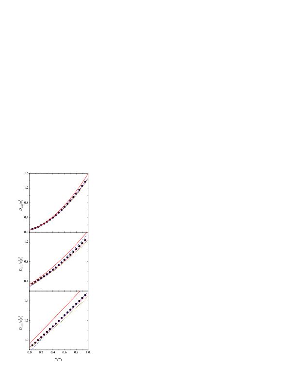
Figure 1: Plot of the composition-independent fourth virial coefficients $D_{1112}$, $D_{1122}$ and $D_{1222}$ versus the size ratio $q=\sigma_{2}/\sigma_{1}$ for a nonadditivity parameter $\Delta=-0.1$. The dotted (green) lines correspond to the original MIX1 theory, Eq. (23), the dash-dot (pink) lines correspond to the mMIX1 theory, Eq. (23), with $Y_{ij}^{\text{M}}\to Y_{ij}^{\text{mM}}$, the dashed (blue) lines correspond to Hamad’s proposal, Eq. (LABEL:2.6), and the solid (red) lines correspond to the SHY proposal, Eq. (28). The symbols are our MC data.

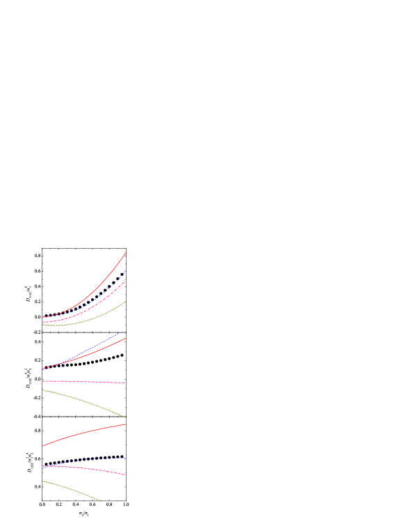
Figure 2: Same as in Fig. 1, but for $\Delta=-0.3$.

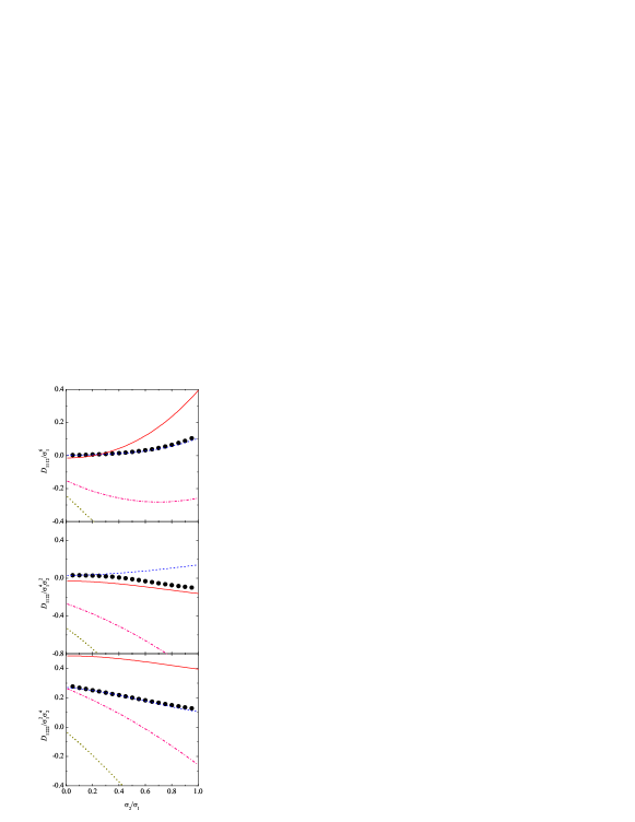
Figure 3: Same as in Fig. 1, but for $\Delta=-0.5$.

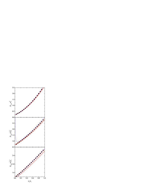
Figure 4: Same as in Fig. 1, but for $\Delta=0.1$.

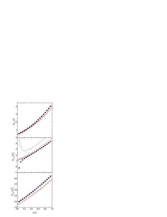
Figure 5: Same as in Fig. 1, but for $\Delta=0.3$.

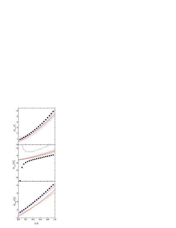
Figure 6: Same as in Fig. 1, but for $\Delta=0.5$.

In this section we report the results of our calculations. In order to evaluate the irreducible cluster integrals which enter the expression of the composition-independent coefficients $D_{ijk\ell}$ [see Eqs. (16) and (17)], we used a standard MC integration procedure. The algorithm produces a significant set of configurations which are compatible with the Mayer graph one wants to evaluate. We first fix particle 1 of species $i$ at the origin and sequentially deposit the remaining three particles at random but in such a way that particle $\alpha+1$ overlaps with particle $\alpha$ (where $\alpha=0,1,2,3$). This procedure generates an open chain of overlapping particles which is taken as a “trial configuration”. A “successful configuration” is a closed-chain configuration (i.e., a configuration in which particle $1$ further overlaps with particle $4$) where, moreover, the residual cross-linked “bonds” which are present in the Mayer graph that is being calculated are also retrieved. The ratio of the number of successful configurations ($N_{s}$) to the total number of trial configurations ($N_{t}$) yields asymptotically the value of the cluster integral relative to that of the open-chain graph which, in turn, is trivially related to a product of the partial second-order virial coefficients $B_{ij}$.Boublík and Nezbeda (1986); Bors̆tnik (1992) The numerical accuracy of the MC results obviously depends on the total number of trial configurations. The error on the cluster integral $J$ is estimated as:Kratky (1977)

$$\text{error}=\left[\frac{J(J-1)}{N_{t}}\right]^{1/2}.$$ (29)

However, as a result of the accumulation of statistically independent errors, the global uncertainty affecting the partial virial coefficients is higher than the error estimated for each cluster integral that enters the expression of $D_{ijk\ell}$. A typical MC run consisted of $4\times 10^{9}$ independent moves. The error on each cluster integral, as estimated through Eq. (29), turned out to be systematically less than $0.05\%$, with a cumulative uncertainty on the partial virial coefficients lower than $0.5\%$.

The numerical values of $D_{1112}/\sigma_{1}^{6}$, $D_{1122}/\sigma_{1}^{6}$, and $D_{1222}/\sigma_{1}^{6}$ for $\Delta=\pm 0.05$, $\pm 0.1$, $\pm 0.2$, $\pm 0.3$, $\pm 0,4$, and $\pm 0.5$ and $q=0.05,0.10,\ldots,0.90,0.95$ are presented in tabular form in the supplementary material to this paper.not (a)

Now we proceed to assess the merits of the different theoretical formulae for the composition-independent partial fourth virial coefficients that we presented in section III. For that purpose, although we have made an exhaustive analysis, in Figs. 1–6 we present only some illustrative cases in which we compare the performance of the different approximations against the MC data. The graphs corresponding to the other values of $\Delta$ that appear in the tables of the supplementary material to this papernot (a) are available upon request.

From these figures it is clear that, overall, the proposal by Hamad,Al-Naafa et al. (1999) Eq. (LABEL:2.6), is very good for $D_{1112}$ and $D_{1222}$ but rather bad for $D_{1122}$ if $|\Delta|>0.1$, irrespective of the value (positive or negative) of $\Delta$. None of the theories shows a good performance in the case of $D_{1122}$ but at least the SHY proposal leads to reasonable quantitative agreement in the positive region of this coefficient, being particularly superior to all other approximations for negative values of $\Delta$.

V Equation of state

Since the convergence of the virial expansion is unknown and truncating the series after the first four terms would not guarantee a satisfactory outcome, in this section we will use the knowledge of the first four virial coefficients to illustrate the performance of a well established approach to the equation of state of fluids that incorporates such knowledge. Hence we will consider the rescaled virial expansion (RVE) proposed by Baus and ColotBaus and Colot (1987); Barrat et al. (1988) to obtain an (approximate) equation of state for an asymmetric NAHD mixture. The RVE equation of state truncated to the fourth order has the following form:

$${Z\equiv\frac{\beta P}{\rho}=\frac{1+c_{1}\eta+c_{2}\eta^{2}+c_{3}\eta^{3}}{(1-\eta)^{2}},}$$ (30)

where $Z$ is the compressibility factor, $\eta=\rho\xi$, with $\xi\equiv(\pi/4)(x_{1}\sigma_{1}^{2}+x_{2}\sigma_{2}^{2})$, is the total packing fraction, and the coefficients $c_{1}$, $c_{2}$, and $c_{3}$ are obtained by identification with the corresponding coefficients which show up in the virial series. Specifically, in the present case one has

$${c_{1}=\frac{B}{\xi}-2,\quad c_{2}=\frac{C}{\xi^{2}}-2\frac{B}{\xi}+1,\quad c_{3}=\frac{D}{\xi^{3}}-2\frac{C}{\xi^{2}}+\frac{B}{\xi}.}$$ (31)

In Fig. 7 we present an illustrative comparison between the results for the compressibility factor of two binary NAHD mixtures as a function of the packing fraction as derived from the RVE, Eq. (30), and those obtained by MC simulation.not (b) In both mixtures the size ratio is $q=0.7$ and a negative nonadditivity $\Delta=-0.2$ (with $x_{1}=0.5$) and a positive nonadditivity $\Delta=0.2$ (with $x_{1}=0.4$) have been considered. For comparison, the results stemming out of the compressibility factors corresponding to the different theoretical approximations mentioned in section III are also included in this figure. As discussed in Ref. Santos et al., 2010, for the actual calculations using the compressibility factors corresponding to the different theoretical approaches, one needs to specify the contact values of the one-component system for the Hamad and the SHY approaches and those of an additive hard-disk mixture in the MIX1 and mMIX theories. For the former we have used an accurate proposal by Luding,Luding (2001); Luding and Santos (2004) while for the latter we have considered the quadratic approximation proposed in Ref. Santos et al., 2002, complemented with Luding’s one-component value.Luding and Santos (2004)

It is clear that in the case of the mixture with negative nonadditivity, the best agreement is provided by both the RVE and the Hamad compressibility factor, followed by the SHY compressibility factor. In fact, the former two are hardly distinguishable. On the other hand, for positive nonadditivity it is the SHY compressibility factor the one that provides the best agreement, followed by both the RVE and the MIX1 compressibility factor. These latter two are virtually indistinguishable.

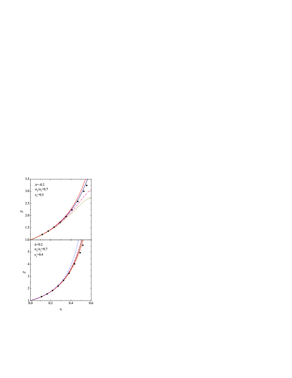
Figure 7: Plot of the compressibility factor $Z$ versus the total packing fraction $\eta$ for NAHD mixtures with $\Delta=-0.2$, $\sigma_{2}/\sigma_{1}=0.7$, $x_{1}=0.5$ (top panel) and $\Delta=0.2$, $\sigma_{2}/\sigma_{1}=0.7$, $x_{1}=0.4$ (bottom panel). The dotted (green) lines correspond to the original MIX1 theory, the dash-dot (pink) lines correspond to the mMIX1 theory, the dashed (blue) lines correspond to Hamad’s proposal, the thick solid (red) lines correspond to the SHY proposal, and the thin solid (black) lines correspond to the RVE, Eq. (30). The symbols are our MC data.not (b) Note that the RVE and the Hamad curves are practically indistinguishable in the top panel, while the RVE and the MIX1 curves are practically indistinguishable in the bottom panel.

VI Concluding remarks

In this paper we have reported MC calculations of the fourth virial coefficients of asymmetric NAHD mixtures over a rather wide range of size ratios $q$ and values of the nonadditivity parameter $\Delta$. These results complement those reported earlierSaija (2011) for symmetric mixtures ($q=1$) and, as illustrated in the case of the RVE and the mixtures discussed in Sec. V, may prove useful for the development of new equations of state for NAHD mixtures. In particular, one could also consider using the availability of the fourth virial coefficients provided in this paper to derive another approximation to the compressibility factor of asymmetric NAHD mixtures via the $y$-expansion proposed by Barboy and Gelbart.Barboy and Gelbart (1979, 1980) Here we have mainly used the data to assess the merits of different theoretical approaches leading to the thermodynamic properties of NAHD mixtures with respect to their performance in the prediction of the values of the fourth virial coefficients.

One immediate conclusion is that none of the existing theories can account for all the features observed in the MC data. In contrast with what happened in NAHS mixtures,Santos et al. (2010) here the theoretical approach by HamadAl-Naafa et al. (1999) outperforms all the rest. In this regard, it is somewhat striking that its very good performance concerning $D_{1112}$ and $D_{1222}$ is not also found for $D_{1122}$, where the SHY proposal does the best overall job. In any case, the comparison we have presented is only indicative of the performance with respect to the fourth virial coefficients, but the full assessment will have to do with the compressibility factor and with the issue of fluid-fluid demixing. We plan to address these points in the near future.