Finite-Element Approximation of
One-Sided Stefan Problems with
Anisotropic, Approximately Crystalline, Gibbs–Thomson Law

Abstract. We present a finite-element approximation for the one-sided Stefan problem and the one-sided Mullins–Sekerka problem, respectively. The problems feature a fully anisotropic Gibbs–Thomson law, as well as kinetic undercooling. Our approximation, which couples a parametric approximation of the moving boundary with a finite-element approximation of the bulk quantities, can be shown to satisfy a stability bound, and it enjoys very good mesh properties, which means that no mesh smoothing is necessary in practice. In our numerical computations we concentrate on the simulation of snow crystal growth. On choosing realistic physical parameters, we are able to produce several distinctive types of snow crystal morphologies. In particular, facet breaking in approximately crystalline evolutions can be observed.

1. Introduction

Pattern formation during crystal growth is one of the most fascinating areas in physics and materials science. Furthermore, crystallisation is a fundamental phase transition, and a good understanding is crucial for many applications. In this paper we will concentrate on a mathematical model based on the one-sided Stefan and Mullins–Sekerka problems, for which we will introduce a new numerical method of approximation. The numerical solutions presented here are tailored for the description of snow crystal growth. However, we note that with minor modifications our approach can be used for other crystal growth scenarios (see [11]), which in particular have applications in engineering as, for example, in the foundry industry.

The basic mathematical model for crystal growth involves diffusion equations in the bulk phases together with complex conditions at the moving boundary, which separates the phases. Depending on the application, either heat diffusion or the diffusion of a solidifying species has to be considered. If a pure, e.g. metallic, substance solidifies, then the basic diffusion equation is the heat equation for the temperature (see [31, 11]), whereas for snow crystal growth the diffusion of water molecules in the air is the main diffusion mechanism (see [33]). In the case that a binary metallic substance solidifies, then models involving both heat and species diffusion simultaneously, and which are coupled through the interface conditions, are considered, see e.g. [16].

At the moving boundary a conservation law either for the energy or for the matter has to hold. In the case of heat diffusion, one has to take into account the release of latent heat through the well-known Stefan condition, which relates the velocity of the interface to the temperature gradients at the interface, the latter being proportional to the energy flux; see [31, 16, 11]. For snow crystal growth the continuity equation at the interface relates its velocity to the particle flux at the interface, which is given in terms of the gradient of the water molecule density. In conclusion, mathematically very similar conditions arise in both models.

Beside the above-discussed continuity equation, another condition has to be specified at the interface. In the case that heat diffusion is the main driving force in the bulk, thermodynamical considerations lead to the Gibbs–Thomson law with kinetic undercooling at the interface; see [31, 16, 11]. This law relates the undercooling (or superheating) at the interface to the curvature and the velocity of the interface. In the case of snow crystal growth one has to consider a modified Hertz–Knudsen formula, which relates the supersaturation of the water molecules at the interface to the curvature and velocity of the interface; see e.g. equations (1) and (23) in [33]. The physics at the interface depends on the local orientation of the crystal lattice in space, and hence the parameters in the interface conditions discussed above are anisotropic. In particular, the corresponding surface energy density leads, through variational calculus, to an anisotropic version of curvature, which then appears in the moving boundary condition; see [23]. In addition, kinetic coefficients in the moving boundary condition will also, in general, be anisotropic.

In the numerical experiments in Section 5, we focus on snow crystal growth, where the unknown will be a properly scaled number density of the water molecules. However, straightforward modifications, e.g. choosing different anisotropies, allow our approach to apply in the context of other crystal growth phenomena. In addition, we note that our approach can be used for many other moving boundary problems; see e.g. [11].

In earlier work, the present authors introduced a new methodology to approximate curvature-driven curve and surface evolution; see [6, 5, 8]. The method has the important feature that mesh properties remain good during the evolution. In fact, for curves semidiscrete versions of the approach lead to polygonal approximations, where the vertices are equally spaced throughout the evolution. This property is important, as most other approaches typically lead to meshes which deteriorate during the evolution and often the computation cannot be continued. The approach was first proposed for isotropic geometric evolution equations, but later the method was generalized to anisotropic situations, [7, 9], and to situations where an interface geometry was coupled to bulk fields, [11]. In most cases it was even possible to show stability bounds. In [11] the two-sided Stefan and Mullins–Sekerka problems, as a model for dendritic solidification, were numerically studied. The physical parameters, such as the heat conductivity, had to be chosen the same in both phases, whereas in this paper we focus on the situation where diffusion can be restricted to the liquid or gas phase, respectively. Hence, we need to study a one-sided Stefan or Mullins–Sekerka problem. This has a significant impact on the numerical analysis, and it necessitates novel computational techniques; see e.g. Section 4.1 below. We remark that an anisotropic version of the one-sided Mullins–Sekerka problem is relevant for snow crystal growth; see [33] and [13]. This, and the fact that the anisotropy in snow crystal growth is so strong that nearly faceted shapes occur, makes this application a perfect situation in order to test whether our approach is suitable for one-sided models for solidification.

Before discussing our numerical approach and several phenomena, which we wish to simulate, we formulate the anisotropic one-sided Stefan and Mullins–Sekerka problem with the Gibbs–Thomson law and kinetic undercooling in detail. Let $\Omega\subset\mathbb{R}^{d}$ be a given domain, where $d=2$ or $d=3$. We now seek a time-dependent interface $(\Gamma(t))_{t\in[0,\overline{T}]}$, $\Gamma(t)\subset\subset\Omega$, which for all $t\in[0,\overline{T}]$ separates $\Omega$ into a domain $\Omega_{+}(t)$, occupied by the liquid/gas, and a domain $\Omega_{-}(t):=\Omega\setminus\overline{\Omega}_{+}(t)$, which is occupied by the solid phase. See Figure 1 for an illustration.

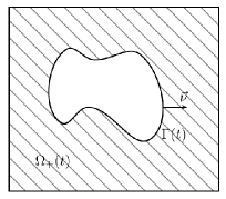
Figure 1. The domain $\Omega$ in the case $d=2$.

For later use, we assume that $(\Gamma(t))_{t\in[0,\overline{T}]}$ is a sufficiently smooth evolving hypersurface parameterized by $\vec{x}(\cdot,t):\Upsilon\to{\mathbb{R}}^{d}$, where $\Upsilon\subset{\mathbb{R}}^{d}$ is a given reference manifold, i.e., $\Gamma(t)=\vec{x}(\Upsilon,t)$. Then $\mathcal{V}:=\vec{x}_{t}\cdot\vec{\nu}$ is the normal velocity of the evolving hypersurface $\Gamma$, where $\vec{\nu}$ is the unit normal on $\Gamma(t)$ pointing into $\Omega_{+}(t)$.

We now need to find a time- and space-dependent function $u$ defined in the liquid/gas region such that $u(\cdot,t):\Omega_{+}(t)\to\mathbb{R}$ and the interface $(\Gamma(t))_{t\in[0,\overline{T}]}$ fulfill the following conditions:

$$\vartheta\,u_{t}-\mathcal{K}\,\Delta u =f\qquad\qquad\qquad \mbox{in }\Omega_{+}(t),$$ (1.1a)

$$\mathcal{K}\,\frac{\partial u}{\partial\vec{\nu}} =-\lambda\,{\mathcal{V}}\qquad \mbox{on }\Gamma(t),$$ (1.1b)

$$\frac{\rho\,\mathcal{V}}{\beta(\vec{\nu})} =\alpha\,\varkappa_{\gamma}-a\,u\qquad \mbox{on }\Gamma(t),$$ (1.1c)

$$u =u_{D}\qquad \mbox{on }\partial\Omega,$$ (1.1d)

$$\Gamma(0) =\Gamma_{0},\qquad\vartheta\,u(\cdot,0)=\vartheta\,u_{0}\qquad \mbox{in }\Omega_{+}(0)\,;$$ (1.1e)

where $\partial\Omega$ denotes the boundary of $\Omega$. In addition, $f$ is a possible forcing term, while $\Gamma_{0}\subset\subset\Omega$ and $u_{0}:\Omega_{+}(0)\to{\mathbb{R}}$ are given initial data. We always assume that the solid region $\Omega_{-}(t)$ is compactly contained in $\Omega$.

The unknown $u$ is, depending on the application, either a temperature or a suitably scaled negative concentration. The orientation-dependent function $\beta$ is a kinetic coefficient, $\gamma$ is the anisotropic surface energy, and $\vartheta\geq 0$, $\mathcal{K},$ $\lambda,$ $\rho,$ $\alpha,$ and $a>0$ are constants whose physical significance is discussed in [11, 13]. For snow crystal growth (see [13]), $-u$ is a suitably scaled concentration with $-u_{D}$ being the scaled supersaturation.

It now remains to introduce the anisotropic mean curvature $\varkappa_{\gamma}$. One obtains $\varkappa_{\gamma}$ as the first variation of an anisotropic interface free energy

$$|\Gamma|_{\gamma}:=\int_{\Gamma}\gamma(\vec{\nu})\;{\rm d}{\mathcal{H}}^{d-1},$$

where $\gamma:{\mathbb{R}}^{d}\to{\mathbb{R}}_{\geq 0}$, with $\gamma(\vec{p})>0$ if $\vec{p}\neq\vec{0}$, is the surface free energy density which depends on the local orientation of the surface via the normal $\vec{\nu}$; and ${\mathcal{H}}^{d-1}$ denotes the $(d-1)$-dimensional Hausdorff measure in ${{\mathbb{R}}}^{d}$. The function $\gamma$ is assumed to be positively homogeneous of degree one, i.e.,

$$\gamma(b\,\vec{p})=b\,\gamma(\vec{p})\quad\forall\ \vec{p}\in{\mathbb{R}}^{d},\ \forall\ b\in{\mathbb{R}}_{>0}\quad\Rightarrow\quad\gamma^{\prime}(\vec{p})\cdot\vec{p}=\gamma(\vec{p})\quad\forall\ \vec{p}\in{\mathbb{R}}^{d}\setminus\{\vec{0}\},$$

where $\gamma^{\prime}$ is the gradient of $\gamma$. The first variation of $|\Gamma|_{\gamma}$ is given by (see e.g. [23] and [9])

$$\varkappa_{\gamma}:=-\nabla_{\!s}\cdot\gamma^{\prime}(\vec{\nu}),$$ (1.2)

where $\nabla_{\!s}.$ is the tangential divergence on $\Gamma$; i.e., we have in particular that

$$\frac{\rm d}{{\rm d}t}\,|\Gamma(t)|_{\gamma}=\frac{\rm d}{{\rm d}t}\,\int_{\Gamma(t)}\gamma(\vec{\nu})\;{\rm d}{\mathcal{H}}^{d-1}=-\int_{\Gamma(t)}\varkappa_{\gamma}\,\mathcal{V}\;{\rm d}{\mathcal{H}}^{d-1}.$$ (1.3)

We remark that in the isotropic case we have that

$$\gamma(\vec{p})=\gamma_{iso}(\vec{p}):=|\vec{p}|\quad\forall\ \vec{p}\in{\mathbb{R}}^{d},$$ (1.4)

which implies that $\gamma(\vec{\nu})=1$; and so $|\Gamma|_{\gamma}$ reduces to $|\Gamma|$, the surface area of $\Gamma$. Moreover, in the isotropic case the anisotropic mean curvature $\varkappa_{\gamma}$ reduces to the usual mean curvature, i.e., to the sum of the principal curvatures of $\Gamma$.

In this paper we are interested in anisotropies of the form

$$\gamma(\vec{p})=\sum_{\ell=1}^{L}\gamma_{\ell}(\vec{p}),\quad\gamma_{\ell}(\vec{p}):=[{\vec{p}\cdot G_{\ell}\,\vec{p}}]^{\frac{1}{2}},$$ (1.5)

where $G_{\ell}\in{\mathbb{R}}^{d\times d}$, for $\ell=1\to L$, are symmetric and positive definite matrices. We note that (1.5) corresponds to the special choice $r=1$ for the class of anisotropies

$$\gamma(\vec{p})=\Big{(}\sum_{\ell=1}^{L}[\gamma_{\ell}(\vec{p})]^{r}\Big{)}^{\frac{1}{r}},$$ (1.6)

which has been considered by the authors in [11]. Numerical methods based on anisotropies of the form (1.6) have first been considered in [7] and [9], and there this choice enabled the authors to introduce unconditionally stable fully discrete finite-element approximations for the anisotropic mean curvature flow, i.e., (1.1c) with $a=0$, and other geometric evolution equations for an evolving interface $\Gamma$. Similarly, in [11], the choice of anisotropies (1.6) leads to fully discrete approximations of the Stefan problem with very good stability properties. We note that the simpler choice $r=1$, i.e., when $\gamma$ is of the form (1.5), leads to a finite-element approximation with a linear system to solve at each time level; see (3.6a–c). In three space dimensions, the choice (1.5) only gives rise to a relatively small class of anisotropies, which is why the authors introduced the more general (1.6) in [9]. For the modelling of snow crystal growth, however, the choice (1.5) is sufficient, and we will stick to this case in the present paper, but we point out that using the method from [11] the approach in this paper can be easily generalized to the more general class of anisotropies in (1.6).

We now give some examples for anisotropies of the form (1.5), which later on will be used for the numerical simulations in this paper. For the visualizations we will use the Wulff shape, [40], defined by

$${\mathcal{W}}:=\{\vec{p}\in{\mathbb{R}}^{d}:\vec{p}\cdot\vec{q}\leq\gamma(\vec{q})\quad\forall\ \vec{q}\in{\mathbb{R}}^{d}\}.$$ (1.7)

Here we recall that the Wulff shape $\mathcal{W}$ is known to be the solution of an isoperimetric problem; i.e., the boundary of $\mathcal{W}$ is the minimizer of $|\cdot|_{\gamma}$ in the class of all surfaces enclosing the same volume; see e.g. [20].

Let $l_{\varepsilon}(\vec{p}):=\left[\varepsilon^{2}\,|\vec{p}|^{2}+p_{1}^{2}\,(1-\varepsilon^{2})\right]^{\frac{1}{2}}$ for $\varepsilon>0$.

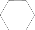
Figure 2. Wulff shape in ${\mathbb{R}}^{2}$ for (1.8) with $\varepsilon=0.01$ and $\theta_{0}=0$.

Then a hexagonal anisotropy in ${\mathbb{R}}^{2}$ can be modelled with the choice

$$\gamma(\vec{p})=\gamma_{hex}(\vec{p}):=\sum_{\ell=1}^{3}l_{\varepsilon}(R(\theta_{0}+\tfrac{\ell\,\pi}{3})\,\vec{p}),$$ (1.8)

where $R(\theta)$ denotes a clockwise rotation through the angle $\theta$, and $\theta_{0}\in[0,\frac{\pi}{3})$ is a parameter that rotates the orientation of the anisotropy in the plane. The Wulff shape of (1.8) for $\varepsilon=0.01$ and $\theta_{0}=0$ is shown in Figure 2.

In order to define anisotropies of the form (1.5) in ${\mathbb{R}}^{3}$, we introduce the rotation matrices

$$R_{1}(\theta):=\left(\begin{array}[]{rrr}\cos\theta&\sin\theta&0\\ -\sin\theta&\cos\theta&0\\ 0&0&1\end{array}\!\!\right)\ \text{ and }\ R_{2}(\theta):=\left(\begin{array}[]{rrr}\cos\theta&0&\sin\theta\\ 0&1&0\\ -\sin\theta&0&\cos\theta\end{array}\!\!\right).$$

Then

$$\gamma(\vec{p})=l_{\varepsilon}(R_{2}(\tfrac{\pi}{2})\,\vec{p})+\sum_{\ell=1}^{3}l_{\varepsilon}(R_{1}(\theta_{0}+\tfrac{\ell\,\pi}{3})\,\vec{p})$$ (1.9)

is one such example, where $\theta_{0}\in[0,\frac{\pi}{3})$ again rotates the anisotropy in the $x_{1}$-$x_{2}$ plane. The anisotropy (1.9) has been used by the authors in their numerical simulations of anisotropic geometric evolution equations in [9, 12, 10], as well as for their dendritic solidification computations in [11]. Its Wulff shape for $\varepsilon=0.01$ is shown on the left of Figure 3.

Figure 3. Scaled Wulff shape in ${\mathbb{R}}^{3}$ for (1.9) with $\varepsilon=0.01$ (left). Scaled Wulff shape in ${\mathbb{R}}^{3}$ for (1.10) with $\varepsilon=0.01$ (right).

A small modification of (1.9), which is more relevant for the simulation of snow flake growth, is

$$\gamma(\vec{p})=\gamma_{hex}(\vec{p}):=l_{\varepsilon}(R_{2}(\tfrac{\pi}{2})\,\vec{p})+\tfrac{1}{\sqrt{3}}\,\sum_{\ell=1}^{3}l_{\varepsilon}(R_{1}(\theta_{0}+\tfrac{\ell\,\pi}{3})\,\vec{p}).$$ (1.10)

Its Wulff shape for $\varepsilon=0.01$ is shown on the right of Figure 3. We note that the Wulff shape of (1.10), in contrast to (1.9), for $\varepsilon\to 0$ approaches a prism where every face has the same distance from the origin. In other words, for (1.10) the surface energy densities in the basal and prismal directions are the same. We remark that if $\mathcal{W}_{0}$ denotes the Wulff shape of (1.10) with $\varepsilon=0$, then the authors in [30] used the scaled Wulff shape $\tfrac{1}{2}\,\mathcal{W}_{0}$ as the building block in their cellular automata algorithm. In addition, we observe that the choice (1.10) agrees well with data reported in e.g. [35, p. 148], although there the ratio of basal to prismal energy is computed as $\gamma^{\rm B}/\gamma^{\rm P}\approx 0.92<1$.

In addition, we consider an example of (1.5), where $L=2$ and $G_{1}=\operatorname{diag}(1,1,\varepsilon^{2})$, $G_{2}=\gamma_{\rm TB}^{2}\,\operatorname{diag}(\varepsilon^{2},\varepsilon^{2},1)$, so that it approximates for small $\varepsilon$ the anisotropy

$$\gamma(\vec{p})=\gamma_{\rm TB}\,|p_{3}|+(p_{1}^{2}+p_{2}^{2})^{\frac{1}{2}},$$ (1.11)

as considered in e.g. [25]. See Figure 4, where we show its Wulff shape for $\gamma_{\rm TB}=1$ and $\gamma_{\rm TB}=0.1$ for $\varepsilon=10^{-2}$.

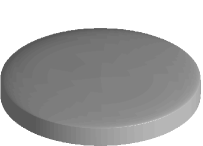
Figure 4. Scaled Wulff shape for the approximation of (1.11) with $\gamma_{\rm TB}=1$ (left) and $\gamma_{\rm TB}=0.1$ (right) for $\varepsilon=10^{-2}$.

We note the Wulff shape of (1.11) is given by a cylinder with basal radius one and height $2\,\gamma_{\rm TB}$. Hence its ratio of height to basal diameter is $\gamma_{\rm TB}$.

More examples of anisotropies of the form (1.6) can be found in [7, 9, 12]. Let us briefly discuss why the novel way that we deal with the anisotropy makes it possible to compute evolution equations resulting from nearly crystalline surface energies, i.e., when the Wulff shape has sharp corners and flat parts. Energies of the form (1.8) and (1.9) have as building blocks simple quadratic expressions, and for $\varepsilon$ close to zero they reduce to crystalline surface energies. It is now possible to discretize these energies, such that the resulting discrete equations are linear and such that they allow for a stability bound; compare Theorem 3.1 below and [7, 9]. Stability bounds for nearly crystalline energies are very difficult to obtain. The fact that we obtain stability bounds for small $\varepsilon$, and hence nearly crystalline energies, together with the good mesh properties of our discrete approximation of the interface enable us to perform numerical computations in situations which involve nearly crystalline surface energies. In this context let us mention that the good mesh quality results from a tangential redistribution of the mesh, where the tangential velocity arises naturally from the discretization of a variational formulation of (1.2).

Crystal growth in general, and snow crystal growth in particular, is a highly anisotropic mechanism. In snow crystal growth the morphologies that appear depend strongly on the environment and, in particular, on the temperature and the supersaturation, which influence the values of $\alpha$ and $u_{D}$, respectively, in (1.1a–e). This can be seen in the famous Nakaya diagram; see Figure 5. Depending on these parameters, either solid prisms, needles, thin plates, hollow columns or dendrites appear in snow crystal growth. The anisotropy of the surface energy can be responsible for the hexagonal symmetry, but probably also an anisotropic $\beta$ has an influence on the shapes appearing in snow crystal growth; see e.g. [33] and [41]. Depending on the size of the crystal, either the kinetic anisotropy or the anisotropy in the surface energy dominates; see [42] or [32]. It is one of the goals of this paper to study the influence of the anisotropies in $\beta$ and $\gamma$ on the growth morphologies. It was discussed in [33] that the kinetic coefficient can vary drastically between the directions of the two basal hexagonal facets and the directions of the six prismal facets. Depending on the environmental conditions either flat crystals or column crystals appear; see Figure 5.

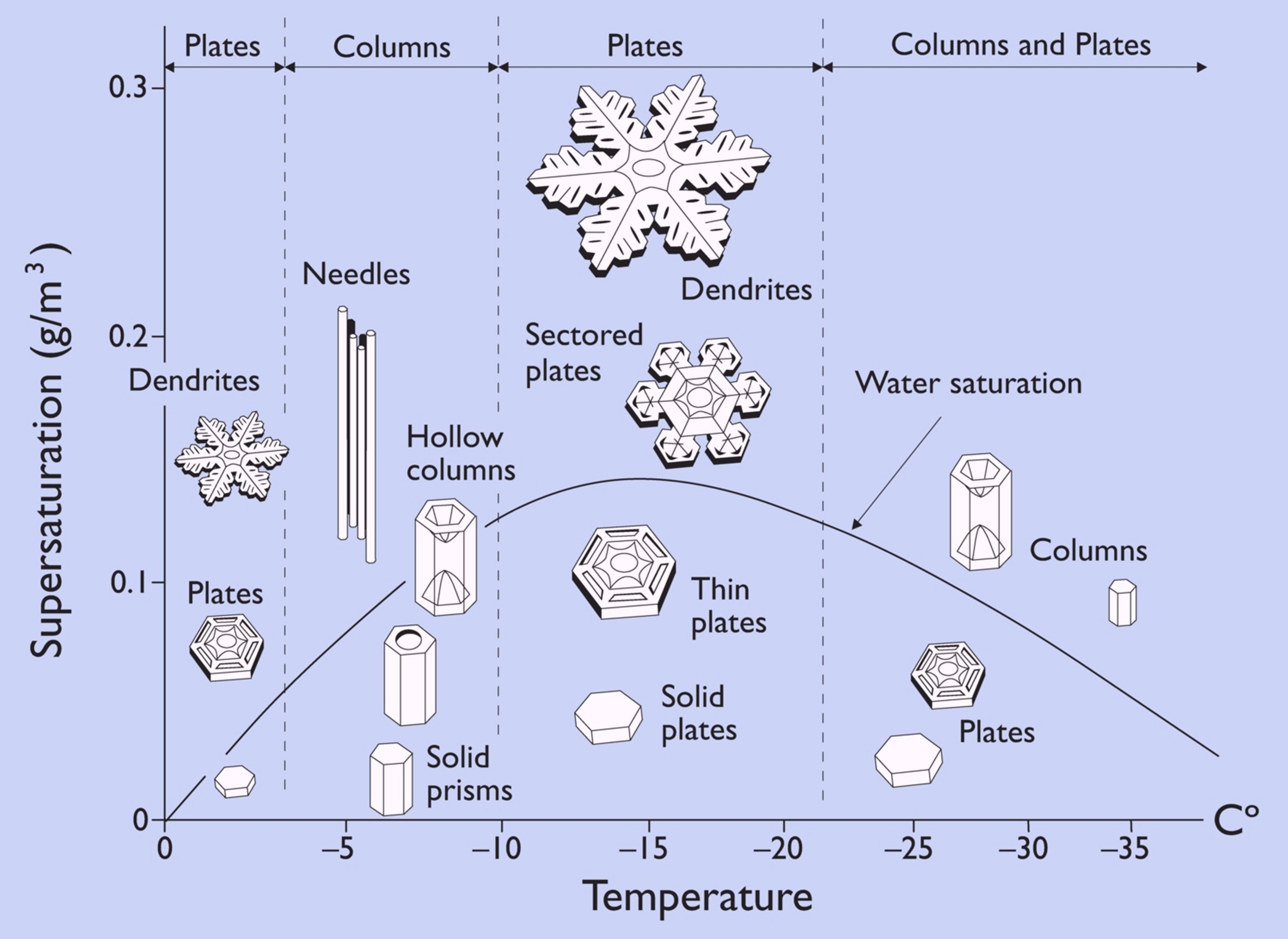
Figure 5. The Nakaya diagram illustrates which snow crystal forms appear at different temperatures and supersaturations. This figure is taken from [33].

A derivation of the set of equations (1.1a–e) can be found in [31] and [16]. The evolution of interfaces driven by anisotropic curvature has been studied by many authors, and we refer to [23] for an overview. For the full problem (1.1a–e), to the knowledge of the authors, no existence result seems to be known, although there are results for two-sided variants; see [34] in the isotropic case and [21] in the anisotropic case. We remark that also cases where the Wulff shape is crystalline have been studied. In this case nonlocal curvature quantities have to be considered, and the geometric equation (1.1c) for the interface is of singular diffusion type. Then local existence to (1.1a–e) has been obtained for anisotropies where the Wulff shape is a prism with polygonal base, for a restricted class of $\Gamma_{0}$ and on assuming that no facet bending or facet breaking occurs; see [28, 29]. In addition, it was shown in [25] that self-similar solutions for (1.1a–e) exist in a situation where the Wulff shape is a cylinder. We will attempt to compute such self-similar solutions in Section 5.

In snow crystal growth often flat parts appear, and in some cases they become unstable and break; see Figure 5, [33] and [27]. Only recently have researchers studied facet breaking from a mathematical point of view. The three-dimensional case has been considered in [15] and [22] for geometrical evolution equations—see also the numerical studies in [9]. A full crystalline model of solidification facet breaking has, so far, only been studied analytically in [26] and numerically in [11]. Clearly from the Nakaya diagram, facet breaking is an important issue in snow crystal growth, and we will study this aspect numerically in Section 5.

Numerical approaches for dendritic solidification that are based on the Stefan problem with the Gibbs–Thomson law are often restricted to two space dimensions; see e.g. [42, 38] and [3], where in the latter article the coupling to a fluid flow is also considered. The first implementations in three space dimensions are due to Schmidt (see [36, 37]), and the present authors later proposed a stable variant of Schmidt’s approach which could also handle the anisotropy in a more physically rigorous way; see [11]. We also would like to refer to the fascinating results on snow crystal growth, which were established in [30], using a cellular automata model. They were able to compute a large variety of forms, which resemble snow crystals in nature, even though the overall approach does not stem from basic physical conservation laws and it is difficult to relate its parameters to physical quantities.

The outline of this paper is as follows. In Section 2 we introduce a weak formulation of the one-sided Stefan problem and the one-sided Mullins–Sekerka problem, which we consider in this paper. Based on this weak formulation, we then introduce our numerical approximation of these problems in Section 3. In particular, on utilizing techniques from [11], we derive a coupled finite-element approximation for the interface evolution and the diffusion equation in the bulk. Moreover, we show well-posedness and stability results for our numerical approximation. Solution methods for the discrete equations and implementation issues are discussed in Section 4. In addition, a non-dimensionalization of a model for snow crystal growth from [33], which allows us to derive physically relevant parameter ranges, is recalled in Section 5.1. Finally, we present several numerical experiments, including simulations of snow crystal formations in three space dimensions, in Section 5.

2. Weak formulation

In this section we state a weak formulation of the problem (1.1a–e) and derive a formal energy bound. Recall that $\vartheta\geq 0$ and $\mathcal{K},\lambda,\rho,\alpha,a>0$ are physical parameters that are discussed in more detail in [11] and in [13].

We introduce the function spaces

$$S_{0,+}(t) :=\{\phi\in H^{1}(\Omega_{+}(t)):\phi=0\ \mbox{ on }\partial\Omega\}$$

$$\quad\mbox{and}\quad S_{D,+}(t) :=\{\phi\in H^{1}(\Omega_{+}(t)):\phi=u_{D}\ \mbox{ on }\partial\Omega\}.$$

In addition, we define $\underline{V}:=H^{1}(\Upsilon,{\mathbb{R}}^{d})$ and $W:=H^{1}(\Upsilon,{\mathbb{R}}),$ where we recall that $\Upsilon$ is a given reference manifold. A possible weak formulation of (1.1a–e), which utilizes the novel weak representation of $\varkappa_{\gamma}\,\vec{\nu}$ introduced in [9], is then given as follows. Find time-dependent functions $u$, $\vec{x}$, and $\varkappa_{\gamma}$ such that $u(\cdot,t)\in S_{D,+}(t)$, $\vec{x}(\cdot,t)\in\underline{V}$, $\varkappa_{\gamma}(\cdot,t)\in W$, and

$$\vartheta\,(u_{t},\phi)_{+}+\mathcal{K}\,(\nabla\,u,\nabla\,\phi)_{+}-(f,\phi)_{+}$$

$$\hskip 14.22636pt=-\mathcal{K}\,\int_{\Gamma(t)}\frac{\partial u}{\partial\vec{\nu}}\,\phi\;{\rm d}{\mathcal{H}}^{d-1}=\lambda\int_{\Gamma(t)}\vec{x}_{t}\cdot\vec{\nu}\,\phi\;{\rm d}{\mathcal{H}}^{d-1}\quad\forall\ \phi\in S_{0,+}(t),$$ (2.1a)

$$\rho\,\int_{\Gamma(t)}\frac{\vec{x}_{t}\cdot\vec{\nu}\,\chi}{\beta(\vec{\nu})}\;\;{\rm d}{\mathcal{H}}^{d-1}=\int_{\Gamma(t)}\left[\alpha\,\varkappa_{\gamma}-a\,u\right]\chi\;{\rm d}{\mathcal{H}}^{d-1}\quad\forall\ \chi\in W,$$ (2.1b)

$$\int_{\Gamma(t)}\varkappa_{\gamma}\,\vec{\nu}\cdot\vec{\eta}\;{\rm d}{\mathcal{H}}^{d-1}+\langle\nabla_{\!s}^{\widetilde{G}}\,\vec{x},\nabla_{\!s}^{\widetilde{G}}\,\vec{\eta}\rangle_{\gamma}=0\quad\forall\ \vec{\eta}\in\underline{V}$$ (2.1c)

hold for almost all times $t\in(0,\overline{T}]$, as well as the initial conditions (1.1e). Here $(\cdot,\cdot)_{+}$ denotes the $L^{2}$-inner product on $\Omega_{+}(t)$.

We note that, for convenience, we have adopted a slight abuse of notation in (2.1a–c). Here, and throughout this paper, we will identify functions defined on the reference manifold $\Upsilon$ with functions defined on $\Gamma(t)$. In particular, we identify $v\in W$ with $v\circ\vec{x}^{-1}$ on $\Gamma(t)$, where we recall that $\Gamma(t)=\vec{x}(\Upsilon,t)$, and we denote both functions simply as $v$. For example, $\vec{x}\equiv\vec{\rm id}$ is also the identity function on $\Gamma(t)$. In addition, we have introduced the shorthand notation $\langle\nabla_{\!s}^{\widetilde{G}}\,\cdot,\nabla_{\!s}^{\widetilde{G}}\,\cdot\rangle_{\gamma}$ for the inner product defined in [9]. In particular, on recalling (1.5), we define the symmetric positive-definite matrices ${\widetilde{G}}_{\ell}$ with the associated inner products $(\cdot,\cdot)_{{\widetilde{G}}_{\ell}}$ on ${\mathbb{R}}^{d}$ by

$${\widetilde{G}}_{\ell}:=[\det G_{\ell}]^{\frac{1}{2}}\,[G_{\ell}]^{-1}\ \mbox{ and }\ (\vec{v},\vec{w})_{{\widetilde{G}}_{\ell}}=\vec{v}\cdot{\widetilde{G}}_{\ell}\,\vec{w}\quad\forall\ \vec{v},\,\vec{w}\in{\mathbb{R}}^{d},\quad\ell=1\to L.$$

Then we have that

$$\langle\nabla_{\!s}^{\widetilde{G}}\vec{\chi},\nabla_{\!s}^{\widetilde{G}}\vec{\eta}\rangle_{\gamma}:=\sum_{\ell=1}^{L}\int_{\Gamma(t)}(\nabla_{\!s}^{{\widetilde{G}}_{\ell}}\vec{\chi},\nabla_{\!s}^{{\widetilde{G}}_{\ell}}\vec{\eta})_{{\widetilde{G}}_{\ell}}\gamma_{\ell}(\vec{\nu})\;{\rm d}{\mathcal{H}}^{d-1}\quad\forall\ \vec{\chi},\vec{\eta}\in\underline{V},$$ (2.2)

where

$$(\nabla_{\!s}^{{\widetilde{G}}_{\ell}}\,\vec{\eta},\nabla_{\!s}^{{\widetilde{G}}_{\ell}}\,\vec{\chi})_{{\widetilde{G}}_{\ell}}:=\sum_{j=1}^{d-1}(\partial_{\vec{t}_{j}^{(\ell)}}\,\vec{\eta},\partial_{\vec{t}_{j}^{(\ell)}}\,\vec{\chi})_{{\widetilde{G}}_{\ell}}$$

with $\{\vec{t}_{1}^{(\ell)},\ldots,\vec{t}_{d-1}^{(\ell)}\}$ being an orthonormal basis with respect to the ${\widetilde{G}}_{\ell}$ inner product for the tangent space of $\Gamma(t)$; see [9] for further details.

Assuming, for simplicity, that the Dirichlet data $u_{D}$ is constant, we can establish the following formal a priori bound. Choosing $\phi=u-u_{D}$ in (2.1a), $\chi=\frac{\lambda}{a}\,\vec{x}_{t}\cdot\vec{\nu}$ in (2.1b), and $\vec{\eta}=\frac{\alpha\,\lambda}{a}\,\vec{x}_{t}$ in (2.1c) we obtain, on using the identities

$$\frac{\rm d}{{\rm d}t}\,\int_{\Omega_{+}(t)}g\;{\rm d}{\mathcal{L}}^{d}=\int_{\Omega_{+}(t)}g_{t}\;{\rm d}{\mathcal{L}}^{d}-\int_{\Gamma(t)}g\,\mathcal{V}\;{\rm d}{\mathcal{H}}^{d-1},$$ (2.3)

with $\mathcal{L}^{d}$ denoting the Lebesgue measure in ${\mathbb{R}}^{d}$ (see e.g. [18]) and

$$\frac{\rm d}{{\rm d}t}\,|\Gamma(t)|_{\gamma}=\frac{\rm d}{{\rm d}t}\,\int_{\Gamma(t)}\gamma(\vec{\nu})\;{\rm d}{\mathcal{H}}^{d-1}=\langle\nabla_{\!s}^{\widetilde{G}}\,\vec{x},\nabla_{\!s}^{\widetilde{G}}\,\vec{x}_{t}\rangle_{\gamma}$$ (2.4)

(see [9]), that

$$\frac{\rm d}{{\rm d}t}\Big{(}\frac{\vartheta}{2}\,|u-u_{D}|^{2}_{\Omega_{+}}+\frac{\alpha\,\lambda}{a}\,|\Gamma(t)|_{\gamma}-\lambda\,u_{D}\,\operatorname{vol}(\Omega_{+}(t))\Big{)}+\mathcal{K}\,(\nabla\,u,\nabla\,u)_{+}$$ (2.5)

$$\hskip 14.22636pt+\frac{\lambda\,\rho}{a}\,\int_{\Gamma(t)}\frac{\mathcal{V}^{2}}{\beta(\vec{\nu})}\;{\rm d}{\mathcal{H}}^{d-1}=-\frac{\vartheta}{2}\,\int_{\Gamma(t)}\mathcal{V}\,|u-u_{D}|^{2}\;{\rm d}{\mathcal{H}}^{d-1}+(f,u-u_{D})_{+},$$

where $|\cdot|_{\Omega_{+}}$ denotes the $L^{2}$-norm on $\Omega_{+}(t)$. In particular, the bound (2.5) for $\vartheta>0$ gives a formal a priori control on $u$ and $\Gamma(t)$ only if $\mathcal{V}\geq 0$, i.e., when the solid region is not shrinking.

3. Finite-element approximation

Let $0=t_{0}<t_{1}<\dots<t_{M-1}<t_{M}=\overline{T}$ be a partitioning of $[0,\overline{T}]$ into possibly variable time steps $\tau_{m}:=t_{m+1}-t_{m}$, $m=0\to M-1$. We set $\tau:=\max_{m=0\to M-1}\tau_{m}$. First we introduce standard finite-element spaces of piecewise-linear functions on $\Omega$.

Let $\Omega$ be a polyhedral domain. For $m\geq 0$, let $\mathcal{T}^{m}$ be a regular partitioning of $\Omega$ into disjoint open simplices, so that $\overline{\Omega}=\cup_{o^{m}\in\mathcal{T}^{m}}\overline{o}^{m}$. Let $J_{\Omega}^{m}$ be the number of elements in $\mathcal{T}^{m}$, so that $\mathcal{T}^{m}=\{o^{m}_{j}:j=1\to J^{m}_{\Omega}\}$. Associated with $\mathcal{T}^{m}$ is the finite-element space

$$S^{m}:=\{\chi\in C(\overline{\Omega}):\chi\!\mid_{o^{m}}\mbox{ is linear }\forall\ o^{m}\in\mathcal{T}^{m}\}\subset H^{1}(\Omega).$$ (3.1)

Let $K_{\Omega}^{m}$ be the number of nodes of $\mathcal{T}^{m}$, and let $\{\vec{p}^{m}_{j}\}_{j=1}^{K_{\Omega}^{m}}$ be the coordinates of these nodes. Let $\{\phi_{j}^{m}\}_{j=1}^{K_{\Omega}^{m}}$ be the standard basis functions for $S^{m}$. We introduce $I^{m}:C(\overline{\Omega})\to S^{m}$, the interpolation operator, such that $(I^{m}\eta)(\vec{p}_{k}^{m})=\eta(\vec{p}_{k}^{m})$ for $k=1\to K_{\Omega}^{m}$. A discrete semi-inner product on $C(\overline{\Omega})$ is then defined by $(\eta_{1},\eta_{2})^{h}_{m}:=(I^{m}[\eta_{1}\,\eta_{2}],1),$ with the induced semi-norm given by $|\eta|_{\Omega,m}:=[\,(\eta,\eta)^{h}_{m}\,]^{\frac{1}{2}}$ for $\eta\in C(\overline{\Omega})$.

The test and trial spaces for our finite-element approximation of the bulk equation (2.1a) are then defined by

$$S^{m}_{0}:=\{\chi\in S^{m}:\chi=0\ \mbox{ on $\partial\Omega$}\}\ \mbox{ and }\ S^{m}_{D}:=\{\chi\in S^{m}:\chi=I^{m}u_{D}\ \mbox{ on $\partial\Omega$}\},$$ (3.2)

where in the definition of $S^{m}_{D}$ we allow for $u_{D}\in H^{\frac{1}{2}}(\partial\Omega)\cap C(\partial\Omega)$. Without loss of generality, let $\{\phi_{j}^{m}\}_{j=1}^{K_{\Omega,D}^{m}}$ be the standard basis functions for $S^{m}_{0}$.

The parametric finite-element spaces in order to approximate $\vec{x}$ and $\varkappa_{\gamma}$ in (2.1a–c), are defined as follows. Similarly to [8], we introduce the following discrete spaces, based on the seminal paper [19]. Let $\Gamma^{m}\subset{\mathbb{R}}^{d}$ be a $(d-1)$-dimensional polyhedral surface, i.e., a union of non-degenerate $(d-1)$-simplices with no hanging vertices (see [18, p. 164] for $d=3$), approximating the closed surface $\Gamma(t_{m})$, $m=0\to M$. In particular, let $\Gamma^{m}=\bigcup_{j=1}^{J^{m}_{\Gamma}}\overline{\sigma}^{m}_{j}$, where $\{\sigma^{m}_{j}\}_{j=1}^{J^{m}_{\Gamma}}$ is a family of mutually disjoint open $(d-1)$-simplices with vertices $\{\vec{q}^{m}_{k}\}_{k=1}^{K^{m}_{\Gamma}}$. Then for $m=0\to M-1$, let

$$\underline{V}(\Gamma^{m}) :=\{\vec{\chi}\in C(\Gamma^{m},{\mathbb{R}}^{d}):\vec{\chi}\!\mid_{\sigma^{m}_{j}}\mbox{ is linear}\ \forall\ j=1\to J^{m}_{\Gamma}\}$$

$$=:[W(\Gamma^{m})]^{d}\subset H^{1}(\Gamma^{m},{\mathbb{R}}^{d}),$$

where $W(\Gamma^{m})\subset H^{1}(\Gamma^{m},{\mathbb{R}})$ is the space of scalar continuous piecewise-linear functions on $\Gamma^{m}$, with $\{\chi^{m}_{k}\}_{k=1}^{K^{m}_{\Gamma}}$ denoting the standard basis of $W(\Gamma^{m})$. For later purposes, we also introduce $\pi^{m}:C(\Gamma^{m},{\mathbb{R}})\to W(\Gamma^{m})$, the standard interpolation operator at the nodes $\{\vec{q}_{k}^{m}\}_{k=1}^{K^{m}_{\Gamma}}$, and similarly $\vec{\pi}^{m}:C(\Gamma^{m},{\mathbb{R}}^{d})\to\underline{V}(\Gamma^{m})$. Throughout this paper, we will parameterize the new closed surface $\Gamma^{m+1}$ over $\Gamma^{m}$, with the help of a parameterization $\vec{X}^{m+1}\in\underline{V}(\Gamma^{m})$, i.e., $\Gamma^{m+1}=\vec{X}^{m+1}(\Gamma^{m})$. Moreover, for $m\geq 0$, we will often identify $\vec{X}^{m}$ with $\vec{\rm id}\in\underline{V}(\Gamma^{m})$, the identity function on $\Gamma^{m}$.

For scalar and vector functions $v,w\in L^{2}(\Gamma^{m},{\mathbb{R}}^{(d)})$ we introduce the $L^{2}$ inner product $\langle\cdot,\cdot\rangle_{m}$ over the current polyhedral surface $\Gamma^{m}$ as follows:

$$\langle v,w\rangle_{m}:=\int_{\Gamma^{m}}v\cdot w\,\;{\rm d}{\mathcal{H}}^{d-1}.$$

Here and throughout this paper, $\cdot^{(\ast)}$ denotes an expression with or without the superscript $\ast$, and similarly for subscripts. If $v$ and $w$ are piecewise continuous, with possible jumps across the edges of $\{\sigma_{j}^{m}\}_{j=1}^{J^{m}_{\Gamma}}$, we introduce the mass lumped inner product $\langle\cdot,\cdot\rangle^{h}_{m}$ as

$$\langle v,w\rangle^{h}_{m}:=\tfrac{1}{d}\sum_{j=1}^{J^{m}_{\Gamma}}|\sigma^{m}_{j}|\sum_{k=1}^{d}(v\cdot w)((\vec{q}^{m}_{j_{k}})^{-}),$$ (3.3)

where $\{\vec{q}^{m}_{j_{k}}\}_{k=1}^{d}$ are the vertices of $\sigma^{m}_{j}$, and where we define $v((\vec{q}^{m}_{j_{k}})^{-}):=\underset{\sigma^{m}_{j}\ni\vec{p}\to\vec{q}^{m}_{j_{k}}}{\lim}\,v(\vec{p})$. Here $|\sigma^{m}_{j}|=\frac{1}{(d-1)!}\,|(\vec{q}^{m}_{j_{2}}-\vec{q}^{m}_{j_{1}})\land\cdots\land(\vec{q}^{m}_{j_{d}}-\vec{q}^{m}_{j_{1}})|$ is the measure of $\sigma^{m}_{j}$, where $\land$ is the standard wedge product on ${\mathbb{R}}^{d}$. Moreover, we set $|\cdot|_{m(,h)}^{2}:=\langle\cdot,\cdot\rangle^{(h)}_{m}$.

Given $\Gamma^{m}$, we let $\Omega^{m}_{+}$ denote the exterior of $\Gamma^{m}$ and let $\Omega^{m}_{-}$ denote the interior of $\Gamma^{m}$, so that $\Gamma^{m}=\partial\Omega^{m}_{-}=\overline{\Omega}^{m}_{-}\cap\overline{\Omega}^{m}_{+}$. In addition, we define the piecewise-constant unit normal $\vec{\nu}^{m}$ to $\Gamma^{m}$ by

$$\vec{\nu}^{m}_{j}:=\vec{\nu}^{m}\!\mid_{\sigma^{m}_{j}}:=\frac{(\vec{q}^{m}_{j_{2}}-\vec{q}^{m}_{j_{1}})\land\cdots\land(\vec{q}^{m}_{j_{d}}-\vec{q}^{m}_{j_{1}})}{|(\vec{q}^{m}_{j_{2}}-\vec{q}^{m}_{j_{1}})\land\cdots\land(\vec{q}^{m}_{j_{d}}-\vec{q}^{m}_{j_{1}})|},$$

where we have assumed that the vertices $\{\vec{q}^{m}_{j_{k}}\}_{k=1}^{d}$ of $\sigma_{j}^{m}$ are ordered such that $\vec{\nu}^{m}:\Gamma^{m}\to{\mathbb{R}}^{d}$ induces an orientation on $\Gamma^{m}$, and such that $\vec{\nu}^{m}$ points into $\Omega^{m}_{+}$.

Before we can introduce our approximation to (2.1a–c), we have to introduce the notion of a vertex normal on $\Gamma^{m}$. We will combine this definition with a natural assumption that is needed in order to show existence and uniqueness, where applicable, for the introduced finite-element approximation.

• We assume for $m=0\to M-1$ that $|\sigma^{m}_{j}|>0$ for all $j=1\to J^{m}_{\Gamma}$, and that $\Gamma^{m}\subset\overline{\Omega}$. For $k=1\rightarrow K^{m}_{\Gamma}$, let $\Xi_{k}^{m}:=\{\sigma^{m}_{j}:\vec{q}^{m}_{k}\in\overline{\sigma}^{m}_{j}\}$ and set

  $$\Lambda_{k}^{m}:=\cup_{\sigma^{m}_{j}\in\Xi_{k}^{m}}\overline{\sigma}^{m}_{j}\qquad\mbox{and}\qquad\vec{\omega}^{m}_{k}:=\frac{1}{|\Lambda^{m}_{k}|}\sum_{\sigma^{m}_{j}\in\Xi_{k}^{m}}|\sigma^{m}_{j}|\;\vec{\nu}^{m}_{j}.$$

  Then we further assume that $\vec{\omega}^{m}_{k}\not=\vec{0}$, $k=1\to K^{m}_{\Gamma}$, and that $\dim\operatorname{span}\{\vec{\omega}^{m}_{k}\}_{k=1}^{K^{m}_{\Gamma}}=d$, $m=0\to M-1$.

Given the above definitions, we also introduce the piecewise-linear vertex normal function

$$\vec{\omega}^{m}:=\sum_{k=1}^{K^{m}_{\Gamma}}\chi^{m}_{k}\,\vec{\omega}^{m}_{k}\in\underline{V}(\Gamma^{m}),$$

and note that

$$\langle\vec{v},w\,\vec{\nu}^{m}\rangle_{m}^{h}=\langle\vec{v},w\,\vec{\omega}^{m}\rangle_{m}^{h}\qquad\forall\ \vec{v}\in\underline{V}(\Gamma^{m}),\ w\in W(\Gamma^{m}).$$ (3.4)

Following [4], we consider the following unfitted finite-element approximation of (2.1a–c). First we need to introduce the appropriate discrete trial and test function spaces. To this end, let $\Omega^{m,h}_{+}$ be an approximation to $\Omega^{m}_{+}$ and set $\Omega^{m,h}_{-}:=\Omega\setminus\overline{\Omega}^{m,h}_{+}$. We stress that $\Omega^{m,h}_{+}$ need not necessarily be a union of elements from $\mathcal{T}^{m}$. Moreover, it need not hold that $\Gamma^{m}\subset\overline{\Omega}^{m,h}_{+}$. Then we define the finite-element spaces

$$S^{m}_{+} :=\{\chi\in S^{m}:\chi(\vec{p}^{m}_{j})=0\text{ if }\operatorname{supp}\phi^{m}_{j}\subset\overline{\Omega}^{m,h}_{-}\},$$

$$\quad S^{m}_{0,+} :=S^{m}_{0}\cap S^{m}_{+},\quad S^{m}_{D,+}:=S^{m}_{D}\cap S^{m}_{+}.$$ (3.5)

Our finite-element approximation is then given as follows. Let $\Gamma^{0}$, an approximation to $\Gamma(0)$, and, if $\vartheta>0$, $U^{0}\in S^{0}_{D}$ be given. For $m=0\to M-1$, find $U^{m+1}\in S^{m}_{D,+}$, $\vec{X}^{m+1}\in\underline{V}(\Gamma^{m})$, and $\kappa^{m+1}_{\gamma}\in W(\Gamma^{m})$ such that for all $\varphi\in S^{m}_{0,+}$, $\chi\in W(\Gamma^{m})$, and $\vec{\eta}\in\underline{V}(\Gamma^{m})$,

$$\vartheta\Big{(}\frac{U^{m+1}-U^{m}}{\tau_{m}},\varphi\Big{)}^{h}_{m,+}+\mathcal{K}\,(\nabla\,U^{m+1},\nabla\,\varphi)_{m,+}$$

$$\hskip 56.9055pt-\lambda\,\Big{\langle}\pi^{m}\Big{[}\frac{\vec{X}^{m+1}-\vec{X}^{m}}{\tau_{m}}\cdot\vec{\omega}^{m}\Big{]},\varphi\Big{\rangle}_{m}=(f^{m+1},\varphi)^{h}_{m,+},$$ (3.6a)

$$\rho\Big{\langle}[\beta(\vec{\nu}^{m})]^{-1}\,\frac{\vec{X}^{m+1}-\vec{X}^{m}}{\tau_{m}},\chi\,\vec{\omega}^{m}\Big{\rangle}_{m}^{h}-\alpha\,\langle\kappa^{m+1}_{\gamma},\chi\rangle_{m}^{h}+a\,\langle U^{m+1},\chi\rangle_{m}=0,$$ (3.6b)

$$\langle\kappa^{m+1}_{\gamma}\,\vec{\omega}^{m},\vec{\eta}\rangle_{m}^{h}+\langle\nabla_{\!s}^{\widetilde{G}}\,\vec{X}^{m+1},\nabla_{\!s}^{\widetilde{G}}\,\vec{\eta}\rangle_{\gamma,m}=0,$$ (3.6c)

and set $\Gamma^{m+1}=\vec{X}^{m+1}(\Gamma^{m})$. Here we define

$$(\nabla\,\chi,\nabla\,\varphi)_{m,+} :=\int_{\Omega^{m,h}_{+}}\nabla\,\chi\cdot\nabla\,\varphi\;{\rm d}{\mathcal{L}}^{d}$$

$$=\sum_{j=1}^{J^{m}_{\Omega}}\tfrac{|o^{m}_{j}\cap\Omega^{m,h}_{+}|}{|o^{m}_{j}|}\,\int_{o^{m}_{j}}\nabla\,\chi\cdot\nabla\,\varphi\;{\rm d}{\mathcal{L}}^{d}\quad\forall\ \chi,\varphi\in S^{m},$$ (3.7a)

and, in a similar fashion,

$$(\chi,\varphi)_{m,+}^{h}:=\sum_{j=1}^{J^{m}_{\Omega}}\tfrac{|o^{m}_{j}\cap\Omega^{m,h}_{+}|}{|o^{m}_{j}|}\,\int_{o^{m}_{j}}I^{m}[\chi\,\varphi]\;{\rm d}{\mathcal{L}}^{d}\quad\forall\ \chi,\varphi\in S^{m}.$$ (3.7b)

For later use we note that it follows immediately from (3.5) and (3.7) that

$$(\nabla\varphi,\nabla\varphi)_{m,+}>0\qquad\forall\ \varphi\in S^{m}_{0,+}\setminus\{0\}.$$ (3.8)

In addition, we set $f^{m+1}(\cdot):=f(\cdot,t_{m+1})$, where we assume for convenience that $f$ is defined on $\Omega$. In addition, for $\vartheta>0$, $U^{0}\in S^{0}_{D}$ is given by $U^{0}=I^{0}[u_{0}]$, where $u_{0}\in C(\overline{\Omega})$ is an appropriately defined extension to $\overline{\Omega}$ of the given initial data from (1.1e).

Moreover, $\langle\nabla_{\!s}^{\widetilde{G}}\,\cdot,\nabla_{\!s}^{\widetilde{G}}\,\cdot\rangle_{\gamma,m}$ in (3.6c) is the discrete inner product defined by

$$\langle\nabla_{\!s}^{\widetilde{G}}\,\vec{\chi},\nabla_{\!s}^{\widetilde{G}}\,\vec{\eta}\rangle_{\gamma,m} :=\sum_{\ell=1}^{L}\int_{\Gamma^{m}}(\nabla_{\!s}^{{\widetilde{G}}_{\ell}}\,\vec{\chi},\nabla_{\!s}^{{\widetilde{G}}_{\ell}}\,\vec{\eta})_{{\widetilde{G}}_{\ell}}\,\gamma_{\ell}(\vec{\nu}^{m})\;{\rm d}{\mathcal{H}}^{d-1}$$

$$\hskip 170.71652pt\forall\ \vec{\chi},\,\vec{\eta}\in\underline{V}(\Gamma^{m}).$$ (3.9)

Note that (3.9) is a natural discrete analogue of (2.2); see [9] for details. This choice of discretization will lead to unconditionally stable approximations in certain situations; see Theorem 3.1, below.

Remark 3.1.

We note that for $\vartheta>0$ the approximation (3.6a–c) is only meaningful when the discrete solid region does not shrink. To see this, assume that the discrete solid region shrinks at some time step, so that $S^{m}_{0,+}\setminus S^{m-1}_{0,+}\not=\emptyset$ for some $m>1$. Assume for simplicity that $\mathcal{T}^{m}=\mathcal{T}^{m-1}$, so that $S^{m}=S^{m-1}$. Now let $\phi^{m}_{j}\in S^{m}_{0,+}\setminus S^{m-1}_{0,+}$, which means that the node $\vec{p}^{m}_{j}$ is an active node in $S^{m}_{0,+}$, but was inactive in $S^{m-1}_{0,+}$; i.e., $U^{m}(\vec{p}^{m}_{j})=0$ since $U^{m}\in S^{m-1}_{D,+}$. Here the value $U^{m}(\vec{p}^{m}_{j})=0$ is arbitrary, and has no physical meaning. Crucially, however, this value will play a role on the discrete level, since choosing $\varphi=\phi^{m}_{j}$ in (3.6a), and noting that $(\phi^{m}_{j},\phi^{m}_{j})^{h}_{m,+}>0$, means that $U^{m+1}$ will depend on $U^{m}(\vec{p}^{m}_{j})$.

In practice this technical restriction is not very relevant, since in physically meaningful simulations the solid region typically never shrinks. Here we also recall that the formal energy bound (2.5), for $\vartheta>0$, is also only meaningful, when the solid region is not shrinking.

Theorem 3.1.

Let the assumption $(\mathcal{A})$ hold. Then there exists a unique solution $(U^{m+1},\vec{X}^{m+1},\kappa^{m+1}_{\gamma})\in S^{m}_{D,+}\times\underline{V}(\Gamma^{m})\times W(\Gamma^{m})$ to (3.6a–c). Let $u_{D}\in{\mathbb{R}}$ and define

$$\mathcal{E}^{m}(U^{m},\vec{X}^{m}):=\frac{\vartheta}{2}\,|U^{m}-u_{D}|_{\Omega,m,+}^{2}+\frac{\alpha\,\lambda}{a}\,|\Gamma^{m}|_{\gamma},$$ (3.10)

where $|\cdot|_{\Omega,m,+}:=[(\cdot,\cdot)^{h}_{m,+}]^{\frac{1}{2}}$. Then the solution to (3.6a–c) satisfies

$$\mathcal{E}^{m}(U^{m+1},\vec{X}^{m+1})+\lambda\,u_{D}\,\langle\vec{X}^{m+1}-\vec{X}^{m},\vec{\omega}^{m}\rangle_{m}^{h}+\frac{\vartheta}{2}\,|U^{m+1}-U^{m}|_{\Omega,m,+}^{2}$$

$$\hskip 5.69046pt+\tau_{m}\,\mathcal{K}\,(\nabla\,U^{m+1},\nabla\,U^{m+1})_{m,+}+\tau_{m}\,\frac{\lambda\,\rho}{a}\Big{|}[\beta(\vec{\nu}^{m})]^{-\frac{1}{2}}\,\frac{\vec{X}^{m+1}-\vec{X}^{m}}{\tau_{m}}\cdot\vec{\omega}^{m}\Big{|}_{m,h}^{2}$$

$$\hskip 56.9055pt\leq\mathcal{E}^{m}(U^{m},\vec{X}^{m})+\tau_{m}\,(f^{m+1},U^{m+1}-u_{D})^{h}_{m,+}.$$ (3.11)

Proof..

As the system (3.6a–c) is linear, existence follows from uniqueness. In order to establish the latter, we consider the following system: Find $(U,\vec{X},\kappa_{\gamma})\in S^{m}_{0,+}\times\underline{V}(\Gamma^{m})\times W(\Gamma^{m})$ such that

$$\vartheta\left(U,\varphi\right)^{h}_{m,+}+\tau_{m}\,\mathcal{K}\,(\nabla\,U,\nabla\,\varphi)_{m,+}-\lambda\left\langle\pi^{m}[\vec{X}\cdot\vec{\omega}^{m}],\varphi\right\rangle_{m}=0\quad\forall\ \varphi\in S^{m}_{0,+},$$ (3.12a)

$$\frac{\rho}{\tau_{m}}\left\langle[\beta(\vec{\nu}^{m})]^{-1}\,\vec{X},\chi\,\vec{\omega}^{m}\right\rangle_{m}^{h}-\alpha\langle\kappa_{\gamma},\chi\rangle_{m}^{h}+a\langle U,\chi\rangle_{m}=0\quad\forall\ \chi\in W(\Gamma^{m}),$$ (3.12b)

$$\langle\kappa_{\gamma}\,\vec{\omega}^{m},\vec{\eta}\rangle_{m}^{h}+\langle\nabla_{\!s}^{\widetilde{G}}\,\vec{X},\nabla_{\!s}^{\widetilde{G}}\,\vec{\eta}\rangle_{\gamma,m}=0\quad\forall\ \vec{\eta}\in\underline{V}(\Gamma^{m}).$$ (3.12c)

Choosing $\varphi=U$ in (3.12a), $\chi=\frac{\lambda}{a}\,\pi^{m}[\vec{X}\cdot\vec{\omega}^{m}]$ in (3.12b), and $\vec{\eta}=\frac{\alpha\,\lambda}{a}\,\vec{X}$ in (3.12c) yields, on noting (3.4), that

$$\vartheta\,(U,U)^{h}_{m,+}+\tau_{m}\,\mathcal{K}\,(\nabla\,U,\nabla\,U)_{m,+}+\frac{\lambda\,\rho}{\tau_{m}\,a}\,\left|[\beta(\vec{\nu}^{m})]^{-\frac{1}{2}}\,\vec{X}\cdot\vec{\omega}^{m}\right|_{m,h}^{2}$$

$$\qquad\qquad\qquad+\frac{\alpha\,\lambda}{a}\,\langle\nabla_{\!s}^{\widetilde{G}}\,\vec{X},\nabla_{\!s}^{\widetilde{G}}\,\vec{X}\rangle_{\gamma,m}=0.$$ (3.13)

It immediately follows from (3.13) and (3.8) that $U=0\in S^{m}_{0,+}$. In addition, on recalling that $\alpha,\lambda>0$, it holds that $\vec{X}\equiv\vec{X}_{c}\in{\mathbb{R}}^{d}$. Together with (3.13), for $U=0$, and the assumption $(\mathcal{A})$ this immediately yields that $\vec{X}\equiv\vec{0}$, while (3.12b) with $\chi=\kappa_{\gamma}$ implies that $\kappa_{\gamma}\equiv 0$; compare Theorem 3.1 in [9]. Hence there exists a unique solution $(U^{m+1},\vec{X}^{m+1},\kappa^{m+1}_{\gamma})\in S^{m}_{D,+}\times\underline{V}(\Gamma^{m})\times W(\Gamma^{m})$.

It remains to establish the bound (3.11). Let $\mathrm{\mathcal{X}}_{\mathcal{A}}$ denote the characteristic function of a set $\mathcal{A}$. Choosing $\varphi=U^{m+1}-u_{D}\,I^{m}\,\mathrm{\mathcal{X}}_{\overline{\Omega}^{m,h}_{+}}$ in (3.6a), $\chi=\frac{\lambda}{a}\,\pi^{m}[({\vec{X}^{m+1}-\vec{X}^{m}})\cdot\vec{\omega}^{m}]$ in (3.6b), and $\vec{\eta}=\frac{\alpha\,\lambda}{a}\,({\vec{X}^{m+1}-\vec{X}^{m}})$ in (3.6c) yields that

$$\vartheta\,(U^{m+1}-U^{m},U^{m+1}-u_{D})^{h}_{m,+}+\tau_{m}\,\mathcal{K}\,(\nabla\,U^{m+1},\nabla\,U^{m+1})_{m,+}$$

$$\hskip 28.45274pt+\frac{\alpha\,\lambda}{a}\,\langle\nabla_{\!s}^{\widetilde{G}}\,\vec{X}^{m+1},\nabla_{\!s}^{\widetilde{G}}\,(\vec{X}^{m+1}-\vec{X}^{m})\rangle_{\gamma,m}$$

$$\hskip 28.45274pt+\tau_{m}\,\frac{\lambda\,\rho}{a}\Big{|}[\beta(\vec{\nu}^{m})]^{-\frac{1}{2}}\,\frac{\vec{X}^{m+1}-\vec{X}^{m}}{\tau_{m}}\cdot\vec{\omega}^{m}\Big{|}_{m,h}^{2}$$

$$\hskip 56.9055pt=-\lambda\,u_{D}\,\langle\vec{X}^{m+1}-\vec{X}^{m},\vec{\omega}^{m}\rangle_{m}^{h}+\tau_{m}\,(f^{m+1},U^{m+1}-u_{D})^{h}_{m,+},$$

and hence (3.11) follows immediately, where we have used the result that

$$\langle\nabla_{\!s}^{\widetilde{G}}\,\vec{X}^{m+1},\nabla_{\!s}^{\widetilde{G}}\,(\vec{X}^{m+1}-\vec{X}^{m})\rangle_{\gamma,m}\geq|\Gamma^{m+1}|_{\gamma}-|\Gamma^{m}|_{\gamma};$$

see e.g. [7] and [9] for the proofs for $d=2$ and $d=3$, respectively. ∎

The above theorem allows us to prove unconditional stability for our scheme under certain conditions.

Theorem 3.2.

Let the assumptions of Theorem 3.1 hold with $u_{D}=0$. In addition, assume that either $\vartheta=0$ or that $U^{m}\in S^{m}_{0}$ and $\Omega^{m,h}_{+}\subset\Omega^{m-1,h}_{+}$ for $m=1\to M-1$. Then it holds that

$$\mathcal{E}^{m}(U^{m+1},\vec{X}^{m+1})$$

$$\hskip 14.22636pt+\sum_{k=0}^{m}\tau_{k}\,\mathcal{K}\Big{[}(\nabla\,U^{k+1},\nabla\,U^{k+1})_{k,+}+\frac{\lambda\,\rho}{a}\Big{|}[\beta(\vec{\nu}^{k})]^{-\frac{1}{2}}\,\frac{\vec{X}^{k+1}-\vec{X}^{k}}{\tau_{k}}\cdot\vec{\omega}^{k}\Big{|}_{k,h}^{2}\Big{]}$$

$$\hskip 113.81102pt\leq\mathcal{E}^{0}(U^{0},\vec{X}^{0})+\sum_{k=0}^{m}\tau_{k}\,(f^{k+1},U^{k+1})^{h}_{k,+}$$ (3.14)

for $m=0\to M-1$.

Proof. The result immediately follows from (3.11) on noting that, if $\vartheta>0$, it follows from our assumptions that $\mathcal{E}^{m}(U^{m},\vec{X}^{m})\leq\mathcal{E}^{m-1}(U^{m},\vec{X}^{m})$ for $m=1\to M-1$, since then

$$\int_{\Omega^{m,h}_{+}}I^{m}[(U^{m})^{2}]\;{\rm d}{\mathcal{L}}^{d} \leq\int_{\Omega^{m-1,h}_{+}}I^{m}[(U^{m})^{2}]\;{\rm d}{\mathcal{L}}^{d}$$

$$=\int_{\Omega^{m-1,h}_{+}}I^{m-1}[(U^{m})^{2}]\;{\rm d}{\mathcal{L}}^{d}.$$ ∎

Remark 3.2.

Theorem 3.2 establishes the unconditional stability of our scheme (3.6a–c) under certain conditions. Of course, if $u_{D}\not=0$, analogous weaker stability results based on (3.11) can be derived. We note that the condition $U^{m}\in S^{m}_{D}$ is trivially satisfied if $S^{m-1}_{D}\subset S^{m}_{D}$, e.g., when mesh refinement routines without coarsening are employed. The condition $\Omega^{m,h}_{+}\subset\Omega^{m-1,h}_{+}$, on the other hand, is ensured whenever the discrete solid region is not shrinking. This is in line with the corresponding continuous energy law (2.5). Note also that the condition $U^{m}\in S^{m}_{D,+}$ would be too strong, as in physically meaningful computations the solid region grows, and so the condition would enforce that $U^{m}=0$ at vertices which are now in the solid region, but were degrees of freedom in $S^{m-1}_{D,+}$. In the simpler case that $\vartheta=0$, the stability bound (3.11) is independent of $U^{m}$, and so here the stability bound (3.14) holds for arbitrary choices of bulk meshes $\mathcal{T}^{m}$.

Remark 3.3.

With the techniques introduced in this paper, it is a simple matter to extend the finite-element approximation introduced in [11] for the two-sided Stefan problem with constant heat conductivity $\mathcal{K}=\mathcal{K}_{s}=\mathcal{K}_{l}$ to the case $\mathcal{K}_{s}-\mathcal{K}_{l}\not=0$, where we have adopted the notation from [11, (2.1a–e)]. Here the subscripts $s$ and $l$ refer to the solid and liquid phase, respectively.

Our finite-element approximation for this problem is then given as follows. Let $\Gamma^{0}$ be given. For $m=0\to M-1$, find $U^{m+1}\in S^{m}_{D}$, $\vec{X}^{m+1}\in\underline{V}(\Gamma^{m})$, and $\kappa^{m+1}_{\gamma}\in W(\Gamma^{m})$ such that for all $\varphi\in S^{m}_{0}$, $\chi\in W(\Gamma^{m})$, and $\vec{\eta}\in\underline{V}(\Gamma^{m})$,

$$\vartheta\Big{(}\frac{U^{m+1}-U^{m}}{\tau_{m}},\varphi\Big{)}^{h}_{m}+\sum_{i\in\{l,s\}}\Big{[}\mathcal{K}_{i}\,(\nabla\,U^{m+1},\nabla\,\varphi)_{m,i}-(f^{m+1}_{i},\varphi)^{h}_{m,i}\Big{]}$$

$$\hskip 113.81102pt-\lambda\,\Big{\langle}\pi^{m}\Big{[}\frac{\vec{X}^{m+1}-\vec{X}^{m}}{\tau_{m}}\cdot\vec{\omega}^{m}\Big{]},\varphi\Big{\rangle}_{m}=0,$$ (3.15a)

$$\rho\Big{\langle}[\beta(\vec{\nu}^{m})]^{-1}\,\frac{\vec{X}^{m+1}-\vec{X}^{m}}{\tau_{m}},\chi\,\vec{\omega}^{m}\Big{\rangle}_{m}^{h}-\alpha\,\langle\kappa^{m+1}_{\gamma},\chi\rangle_{m}^{h}+a\,\langle U^{m+1},\chi\rangle_{m}=0,$$ (3.15b)

$$\langle\kappa^{m+1}_{\gamma}\,\vec{\omega}^{m},\vec{\eta}\rangle_{m}^{h}+\langle\nabla_{\!s}^{\widetilde{G}}\,\vec{X}^{m+1},\nabla_{\!s}^{\widetilde{G}}\,\vec{\eta}\rangle_{\gamma,m}=0,$$ (3.15c)

and set $\Gamma^{m+1}=\vec{X}^{m+1}(\Gamma^{m})$. Here $(\nabla\,\chi,\nabla\,\varphi)_{m,i}$ and $(\chi,\varphi)_{m,i}^{h}$, for $i\in\{s,l\}$ and for $\chi,\varphi\in S^{m}$, are defined analogously to (3.7,b), where $\Omega^{m,h}_{l}:=\Omega^{m,h}_{+}$ and $\Omega^{m,h}_{s}:=\Omega^{m,h}_{-}$ represent approximations to the “liquid” and “solid” phases in this two-sided Stefan problem.

4. Solution of the discrete system

Introducing the obvious abuse of notation, the linear system (3.6a–c) can be formulated as follows: Find $(U^{m+1},\kappa^{m+1}_{\gamma},\delta\vec{X}^{m+1})$ such that

$$\begin{pmatrix}\frac{1}{\tau_{m}}\,M_{\Omega}+A_{\Omega}&0&-\frac{\lambda}{\tau_{m}}\,\vec{N}_{\Gamma,\Omega}^{T}\\ -a\,M_{\Gamma,\Omega}&\alpha\,M_{\Gamma}&-\frac{\rho}{\tau_{m}}\,[\vec{N}_{\Gamma}^{(\beta)}]^{T}\\ 0&\vec{N}_{\Gamma}&\vec{A}_{\Gamma}\end{pmatrix}\begin{pmatrix}U^{m+1}\\ \kappa^{m+1}_{\gamma}\\ \delta\vec{X}^{m+1}\end{pmatrix}=\begin{pmatrix}\frac{1}{\tau_{m}}\,M_{\Omega}\,U^{m}+g^{m}\\ 0\\ -\vec{A}_{\Gamma}\,\vec{X}^{m}\end{pmatrix},$$ (4.1)

where $(U^{m+1},\kappa^{m+1}_{\gamma},\delta\vec{X}^{m+1})\in{\mathbb{R}}^{K^{m}_{\Omega}}\times{\mathbb{R}}^{K^{m}_{\Gamma}}\,\times({\mathbb{R}}^{d})^{K^{m}_{\Gamma}}$ here denote the coefficients of these finite-element functions with respect to the standard bases of $S^{m}$, $W(\Gamma^{m})$, and $\underline{V}(\Gamma^{m})$, respectively. The definitions of the matrices in (4.1) directly follow from (3.6a–c), but we state them here for completeness. Let $i,j=1\to K_{\Omega}^{m}$ and $k,l=1\to K^{m}_{\Gamma}$. Then, on recalling (3.2), we have that

$$[M_{\Omega}]_{ij}:=\vartheta\,(\phi_{j}^{m},\phi_{i}^{m})^{h}_{m,+},$$

$$[\widetilde{A}_{\Omega}]_{ij}:=\begin{cases}\mathcal{K}\,(\nabla\,\phi_{j}^{m},\nabla\,\phi_{i}^{m})_{m,+}&1\leq i\leq K^{m}_{\Omega,D}\\ \delta_{i,j}&K^{m}_{\Omega,D}<i\leq K^{m}_{\Omega}\end{cases},$$

$$[M_{\Gamma,\Omega}]_{li}:=\langle\phi_{i}^{m},\chi^{m}_{l}\rangle_{m},$$

$$[\vec{N}_{\Gamma,\Omega}]_{li}:=\left(\langle\phi_{i}^{m},\pi^{m}\left[(\chi^{m}_{l}\,\vec{e}_{j})\cdot\vec{\omega}^{m}\right]\rangle_{m}\right)_{j=1}^{d}=\langle\phi_{i}^{m},\chi^{m}_{l}\rangle_{m}\,\vec{\omega}^{m}_{l},$$

$$[M_{\Gamma}]_{kl}:=\langle\chi^{m}_{l},\chi^{m}_{k}\rangle_{m}^{h},\quad[\vec{A}_{\Gamma}]_{kl}:=\left(\langle\nabla_{\!s}^{\widetilde{G}}\,(\chi^{m}_{l}\,\vec{e}_{i}),\nabla_{\!s}^{\widetilde{G}}\,(\chi^{m}_{k}\,\vec{e}_{j})\rangle_{\gamma,m}\right)_{i,j=1}^{d},$$

$$[\vec{N}_{\Gamma}]_{kl}:=\langle\chi^{m}_{l},\chi^{m}_{k}\,\vec{\omega}^{m}\rangle_{m}^{h},$$

$$[\vec{N}^{(\beta)}_{\Gamma}]_{kl}:=\langle[\beta(\vec{\nu}^{m})]^{-1}\chi^{m}_{l},\chi^{m}_{k}\,\vec{\omega}^{m}\rangle_{m}^{h}=\langle[\beta(\vec{\nu}^{m})]^{-1}\chi^{m}_{l},\chi^{m}_{k}\rangle_{m}^{h}\,\vec{\omega}^{m}_{l},$$ (4.2)

where $\{\vec{e}_{i}\}_{i=1}^{d}$ denotes the standard basis in ${\mathbb{R}}^{d}$ and where we have used the convention that the subscripts in the matrix notation refer to the test and trial domains, respectively. A single subscript is used where the two domains are the same. We note that the special definition of $\widetilde{A}_{\Omega}$, together with $g^{m}$ in (4.1), accounts for the Dirichlet boundary conditions of $U^{m+1}\in S^{m}_{D}$. Here $g^{m}$ is defined by

$$g^{m}_{i}=\begin{cases}(f^{m+1},\phi^{m}_{i})^{h}_{m,+}&1\leq i\leq K^{m}_{\Omega,D},\\ u_{D}&K^{m}_{\Omega,D}<i\leq K^{m}_{\Omega}.\end{cases}$$ (4.3)

Clearly, the matrix $\widetilde{A}_{\Omega}$ will in general be singular. In particular, it will have zero diagonal entries for every vertex $\vec{p}^{m}_{j}\in\overline{\Omega}^{m,h}_{-}$. Hence we enforce $U^{m+1}\in S^{m}_{D,+}$ by setting

$$[A_{\Omega}]_{ij}=\begin{cases}[\widetilde{A}_{\Omega}]_{ij}&[\widetilde{A}_{\Omega}]_{ij}\not=0,\\ \delta_{i,j}&[\widetilde{A}_{\Omega}]_{ij}=0\,;\end{cases}$$ (4.4)

i.e., we replace zero diagonal entries by $1$.

The assembly of the matrices in (4.2), apart from $\widetilde{A}_{\Omega}$, is described in [11, Section 4]. The assembly of $\widetilde{A}_{\Omega}$, and in particular the possible definitions of the region $\Omega^{m,h}_{+}$, will be discussed in Section 4.1 below. The linear system (4.1) can be efficiently solved with iterative solvers applied to a Schur complement formulation; see [11] for details. For completeness we state that for the application of preconditioners and for the solution of subproblems we make use of the packages LDL and AMD; see [17, 1].

4.1. Definition of the discrete liquid/gas region

We now discuss possible choices of $\Omega^{m,h}_{+}$ in (3.5) and (3.7,b). To this end, we partition the elements of the bulk mesh $\mathcal{T}^{m}$ into liquid/gas, solid, and interfacial elements as follows. Let

$$\mathcal{T}^{m}_{+} :=\{o^{m}\in\mathcal{T}^{m}:\overline{o}^{m}\subset\Omega^{m}_{+}\},\ \quad\ \mathcal{T}^{m}_{-}:=\{o^{m}\in\mathcal{T}^{m}:\overline{o}^{m}\subset\Omega^{m}_{-}\},$$

$$\mathcal{T}^{m}_{\Gamma^{m}} :=\{o^{m}\in\mathcal{T}^{m}:\overline{o}^{m}\cap\Gamma^{m}\not=\emptyset\}.$$ (4.5)

Then $\mathcal{T}^{m}=\mathcal{T}^{m}_{+}\cup\mathcal{T}^{m}_{-}\cup\mathcal{T}^{m}_{\Gamma^{m}}$ is a disjoint partition.

Clearly, using $\Omega^{m,h}_{+}=\Omega^{m}_{+}$ is not very practical, since the intersection of $\Omega^{m}_{+}$ with elements of the bulk mesh $\mathcal{T}^{m}$ can be complicated. Moreover, computing the domain $\Omega^{m}_{+}$ is unlikely to be rewarded with lower overall approximation errors, since the trial and test functions in (3.7,b) are only piecewise linear. Instead, we consider the following approach, which defines $\Omega^{m,h}_{+}$ with the help of a piecewise-linear approximation to $\mathrm{\mathcal{X}}_{\overline{\Omega}^{m}_{+}}$ as

$$\Omega^{m,h}_{+}:=\{\vec{p}\in\Omega:(I^{m}\,\mathrm{\mathcal{X}}_{\overline{\Omega}^{m}_{+}})(\vec{p})>0\}.$$ (4.6)

Next we discuss an algorithm that computes $\Omega^{m,h}_{+}$ for the strategy (4.6). Here each element of $\mathcal{T}^{m}$ is assigned to one of the three sets $\mathcal{T}^{m}_{+}$, $\mathcal{T}^{m}_{-}$, or $\mathcal{T}^{m}_{\Gamma^{m}}$ as described in Algorithm 4.1.

Algorithm 4.1 Mark all bulk mesh elements as liquid/gas, solid, or cut.

1. Traversing over $\Gamma^{m}$, find all elements of $\mathcal{T}^{m}_{\Gamma^{m}}$.
2. Set $\mathcal{T}:=\mathcal{T}^{m}\setminus\mathcal{T}^{m}_{\Gamma^{m}}$ and $\mathcal{T}^{m}_{+}:=\emptyset$.
3. Move all elements that touch $\partial\Omega$ from $\mathcal{T}$ to $\mathcal{T}^{m}_{+}$.
4. For as long as this is possible, move neighbours of elements in $\mathcal{T}^{m}_{+}$ from
 $\mathcal{T}$ to $\mathcal{T}^{m}_{+}$.
5. Set $\mathcal{T}^{m}_{-}:=\mathcal{T}$.

In addition, for later use, we need to decide for each bulk mesh vertex $\vec{p}_{j}^{m}$, $j=1\to K^{m}_{\Omega}$, whether it belongs to $\overline{\Omega}^{m}_{+}$ or to $\overline{\Omega}^{m}_{-}$. This can be done as described in Algorithm 4.2.

Algorithm 4.2 Assign all bulk mesh vertices to $\overline{\Omega}^{m}_{-}$ or $\overline{\Omega}^{m}_{+}$.

1. All vertices of elements in $\mathcal{T}^{m}_{-}$ belong to $\overline{\Omega}^{m}_{-}$.
2. All vertices of elements in $\mathcal{T}^{m}_{+}$ belong to $\overline{\Omega}^{m}_{+}$.
3. For any remaining vertices $\{\vec{p}_{j}^{m}\}$, choose a $\vec{p}^{m}_{j}$ with a neighbouring
 vertex $\vec{q}$ that is known to belong to $\overline{\Omega}^{m}_{-}$ or $\overline{\Omega}^{m}_{+}$. If $\Gamma^{m}$ cuts the
 segment $[\vec{p}_{j}^{m},\vec{q}]\subset{\mathbb{R}}^{d}$ an even number of times, assign $\vec{p}_{j}^{m}$ to the same
 region as $\vec{q}$, otherwise to the opposite region. Repeat this, until all
 vertices have been assigned.

Remark 4.1.

The global Algorithm 4.1 is only needed at the very first time step. For subsequent time steps, the existing marking of bulk mesh elements can be updated depending on the movement of $\Gamma^{m}$. In particular, only elements in $\mathcal{T}^{m-1}_{\Gamma^{m-1}}\setminus\mathcal{T}^{m}_{\Gamma^{m}}$ need to be considered. On assuming that $\Gamma^{m}$ has not travelled over a whole bulk mesh element, these elements can be marked with the help of neighbour information. This is far more efficient than employing the global Algorithm 4.1 at every time step.

In addition, in practice for a refined bulk mesh in the neighbourhood of $\Gamma^{m}$, all the remaining vertices in Step 3 of Algorithm 4.2 have immediately a neighbouring vertex $\vec{q}$ that is known to belong to $\overline{\Omega}^{m}_{-}$ or $\overline{\Omega}^{m}_{+}$.

An alternative approach to (4.6) would not define $\Omega^{m,h}_{+}$ explicitly, but rather the effect of $\Omega^{m,h}_{+}$ on the inner products defined in (3.7,b). Here it is natural to define $\Omega^{m,h}_{+}$ in such a way, that $\bigcup_{o^{m}\in\mathcal{T}^{m}_{-}}\overline{o}^{m}\subset\overline{\Omega}^{m,h}_{-}$. Then the integral in (3.7) can be rewritten as

$$(\nabla\chi,\nabla\,\varphi)_{m,+}=\!\!\!\!\!\sum_{o^{m}\in\mathcal{T}^{m}_{+}}\int_{o^{m}}\!\!\!\nabla\,\chi.\nabla\,\varphi\;{\rm d}{\mathcal{L}}^{d}+\!\!\!\!\!\sum_{o^{m}\in\mathcal{T}^{m}_{\Gamma^{m}}}v(o^{m})\int_{o^{m}}\!\!\!\nabla\chi.\nabla\varphi\;{\rm d}{\mathcal{L}}^{d},$$ (4.7)

where $v(o^{m})\in[0,1]$ denotes the fraction of the element $o^{m}$ that is considered to belong to the liquid/gas region $\Omega^{m,h}_{+}$, and similarly for the inner product defined in (3.7b). Note that (4.7) only implicitly defines (candidates of) the region $\Omega^{m,h}_{+}$.

In practice, several choices of $v(o^{m})\in[0,1]$ can be considered. The approach (4.6) corresponds to

$$v(o^{m})=1\qquad\forall\ o^{m}\in\mathcal{T}^{m}_{\Gamma^{m}},$$ (4.8a)

while the choice

$$v(o^{m})=0\qquad\forall\ o^{m}\in\mathcal{T}^{m}_{\Gamma^{m}}$$ (4.8b)

was used in [3] for a two-sided Stefan problem with nonvanishing heat conductivity coefficients. We note that for the one-sided situation considered in this paper, the strategy (4.8b) does not make sense, as it dramatically affects the accuracy of the approximation $$U^{m+1} \Gamma^{m}$$ on . An alternative approach is the choice

$$v(o^{m})=\tfrac{k}{d+1}=\frac{1}{|o^{m}|}\int_{o^{m}}I^{m}\,\mathrm{\mathcal{X}}_{\overline{\Omega}^{m}_{+}}\;{\rm d}{\mathcal{L}}^{d}\qquad\forall\ o^{m}\in\mathcal{T}^{m}_{\Gamma^{m}},$$ (4.8c)

where $$k \overline{o}^{m} \overline{\Omega}^{m}_{+}$$ denotes the number of vertices of that lie within . A simpler approach is to set

$$v(o^{m})=\tfrac{1}{2}\qquad\forall\ o^{m}\in\mathcal{T}^{m}_{\Gamma^{m}}.$$ (4.8d)

We note that for the practical implementation, the strategies (4.8a,b,d) only need the marking from Algorithm 4.1. The additional Algorithm 4.2 is only required for the strategy (4.8c). In practice, the three strategies (4.8a,c,d) all show very similar numerical results. Hence, in general we will employ the simplest strategy (4.8a).

Remark 4.2.

Of course, setting

$$v(o^{m})=|o^{m}\cap\Omega^{m}_{+}|\qquad\forall\ o^{m}\in\mathcal{T}^{m}_{\Gamma^{m}}$$ (4.9)

corresponds to $\Omega^{m,h}_{+}=\Omega^{m}_{+}$. This will in general be too costly to do in practice. However, we mention one possible strategy here. For an arbitrary open bounded set $V\subset{\mathbb{R}}^{d}$ with Lipschitz boundary it holds that

$$\operatorname{vol}(V)=\int_{V}1\;{\rm d}{\mathcal{L}}^{d}=\tfrac{1}{d}\,\int_{\partial V}(\vec{\rm}id-\vec{z}_{0})\cdot\vec{\nu}_{V}\;{\rm d}{\mathcal{H}}^{d-1},$$ (4.10)

where $\vec{\rm}id$ is the identity function on ${\mathbb{R}}^{d}$, $\vec{z}_{0}\in{\mathbb{R}}^{d}$ is an arbitrarily fixed point, and where $\vec{\nu}_{V}$ denotes the outer normal to $V$. Applying (4.10) for $V=o^{m}\cap\Omega^{m}_{+}$, on noting that $\vec{\nu}_{V}=-\vec{\nu}^{m}$ on $o^{m}\cap\Gamma^{m}$ and $\vec{\nu}_{V}=\vec{\nu}_{o^{m}}$, the outer normal of $o^{m}$, on $\partial o^{m}\cap\Omega^{m}_{+}$, yields a way of using (4.9) in practice. Of course, in this case $V$ is a polytope, with $\partial V$ being a union of flat facets. Thus the integral in (4.10) simplifies on noting that $\vec{\rm}id\cdot\vec{\nu}_{V}$ is now constant on each facet, and vanishes on each facet that contains $\vec{z}_{0}$. Moreover, $o^{m}\cap\Gamma^{m}$ can be computed as in [11, Section 4.5]. It remains to calculate $\partial o^{m}\cap\Omega^{m}_{+}$, where for our purposes it is enough to compute $|F_{\mu}\cap\Omega^{m}_{+}|$ for $\mu=1\to d+1$, where $F_{\mu}$ are the edges/faces of $o^{m}$; i.e., $\partial o^{m}=\cup_{\mu=1}^{d+1}\overline{F}_{\mu}$. For $d=2$ this reduces to finding the lengths of $F_{\mu}\cap\Omega^{m}_{+}$, which is straightforward. For $d=3$ the set $F_{\mu}\cap\Omega^{m}_{+}$ in general can be the disjoint union of possibly non-convex polygons. The oriented boundary of these polygons can be found by suitably arranging the line segments making up $\partial F_{\mu}\cap\Gamma^{m}$, as well as the line segments making up $\partial F_{\mu}\cap\Omega^{m}_{+}$. Then the area $|F_{\mu}\cap\Omega^{m}_{+}|$ can be easily computed with Gauss’ area formula.

5. Numerical results

We implemented our finite-element approximation (3.6a–c) within the framework of the finite-element toolbox ALBERTA; see [39]. We use the bulk mesh and parametric mesh refinement strategies introduced in [11, Section 5]. Here the bulk mesh adaptation algorithm, which was inspired by a similar strategy proposed in [14] and [2] for $d=2$ and $d=3$, respectively, results in a fine mesh of uniform mesh size $h_{f}$ around $\Gamma^{m}$ and a coarse mesh of uniform mesh size $h_{c}$ further away from it. Here $h_{f}=\frac{2\,H}{N_{f}}$ and $h_{c}=\frac{2\,H}{N_{c}}$ are given by two integer numbers $N_{f}>N_{c}$, where we assume from now on that $\Omega=(-H,H)^{d}$. For the one-sided problems considered in this paper, we slightly amend the strategy from [11, Section 5], in that we allow an even coarser grid inside $\Omega^{m,h}_{-}$. Of course, the definitions (3.5) mean that this has no effect on the numerical results. Moreover, the parametric mesh refinement uses bisections in order to avoid elements getting too large over time. We stress that apart from this simple mesh refinement, no other changes were performed on the parametric mesh in any of our simulations. In particular, no mesh smoothing (redistribution) was required.

Throughout this section we use (almost) uniform time steps, in that $\tau_{m}=\tau$, $m=0\to M-2$, and $\tau_{M-1}=T-t_{m-1}\leq\tau$. Unless otherwise stated we set $\Omega=(-H,H)^{d}$ with $H=4$. Similarly, unless otherwise stated, we always employ the strategy (4.8a) for the computation of $\Omega^{m,h}_{+}$. The initial interface $\Gamma(0)$ is always a circle/sphere of radius $R_{0}\in(0,H)$ around the origin. For the Stefan problem, i.e., if $\vartheta>0$, we set

$$u_{0}(\vec{z})=\begin{cases}0&|\vec{z}|\leq R_{0},\\ \dfrac{1-e^{R_{0}-|\vec{z}|}}{1-e^{R_{0}-H}}\,u_{D}&R_{0}<|\vec{z}|<H,\\ u_{D}&|\vec{z}|\geq H,\end{cases}$$ (5.1)

unless a true solution $u$ is given.

For later purposes, we define

$$\vec{X}(t):=\tfrac{t-t_{m-1}}{\tau_{m}}\,\vec{X}^{m}+\tfrac{t_{m}-t}{\tau_{m-1}}\vec{X}^{m-1},\ \ t\in[t_{m-1},t_{m}],\ \ m\geq 1,$$

and similarly for $U$.

5.1. Non-dimensionalization of a model for snow crystal growth

An aim of this paper is to be able to perform computations for the growth of snow crystals with realistic parameters and on physically relevant length and time scales. Upon non-dimensionalizing the continuum model for snow crystal growth from [33], it turns out that (1.1a–c) with

$$\vartheta=0,\ \ \mathcal{K}=1,\ \ \lambda=1,\ \ \rho=1.42\times 10^{-3},\ \ \alpha=10^{-5},\ \ a=1,\ \ f=0$$ (5.2)

is a physically realistic model. Here the typical length scale is 100 $\mu$m, typical time scales vary from 100 s to 1300 s, $-u$ denotes a scaled concentration of water vapour in the gas phase, and $-u_{D}$ is a scaled supersaturation. We refer to [13] for more details on the physical interpretation of these parameters.

5.2. Convergence experiments

We begin with a comparison of the approximation error $\operatorname{vol}(\Omega_{+}(0))-\operatorname{vol}(\Omega^{0,h}_{+})$ for the four different strategies (4.8a–d). Here we set $\Omega_{+}(0)=\overline{\Omega}\setminus B_{1}(0)$ and, for the case $d=2$, use the spatial discretization parameters $N_{f}=K^{0}_{\Gamma}=2^{7+i}$ and $N_{c}=4^{i}$. An example of how the discrete interface $\Gamma^{0}$ cuts the bulk mesh $\mathcal{T}^{0}$ is shown in Figure 6.

The numerical results are shown in Table 1, where we observe that the strategies (4.8c,d) produce far smaller errors than (4.8a,b). However, as we will see in the subsequent convergence experiments, this does not seem to have an influence on the overall approximation error for the underlying solutions $u$ and $\Gamma$.

For completeness, we repeat the same experiments for $d=3$, where now $N_{f}=2^{6+i}$, $N_{c}=4^{i}$, and $K^{0}_{\Gamma}=K(i)$, with $(K(0),K(1),K(2),K(3))=(770,3074,12290,49154)$, for $i=0\to 3$. The results are shown in Table 2.

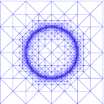
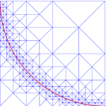
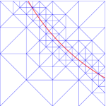
Figure 6. Parts of the triangulation $\mathcal{T}^{0}$ and the interface $\Gamma^{0}$ when $N_{f}=K^{0}_{\Gamma}=2^{8}$ and $N_{c}=4$. From left to right $[-2,2]^{2}$, $[-1,0]^{2}$, and $[-1,-\frac{1}{2}]^{2}$.

$10^{3}\,h_{f}$	$h^{M}_{\Gamma}$	(4.8a)	(4.8c)	(4.8d)	(4.8b)
62.500	5.4874e-02	-2.3534e-01	-1.1384e-02	-8.7802e-03	2.1778e-01
31.250	2.7439e-02	-1.1425e-01	-4.8739e-03	-4.8739e-03	1.0450e-01
15.625	1.3720e-02	-5.5655e-02	-1.9442e-03	-1.4559e-03	5.2743e-02
7.8125	6.8600e-03	-2.7579e-02	-1.2118e-03	-7.2351e-04	2.6132e-02
3.9062	3.4300e-03	-1.4273e-02	-7.0317e-04	-8.7610e-04	1.2521e-02

Table 1. $\Omega=(-4,4)^{2}$. Approximation error $\operatorname{vol}(\Omega_{+}(0))-\operatorname{vol}(\Omega^{0,h}_{+})$ for (4.8a–d).

$10^{2}\,h_{f}$	$h^{M}_{\Gamma}$	(4.8a)	(4.8c)	(4.8d)	(4.8b)
12.500	2.0854e-01	-8.9192e-01	-6.7696e-02	-1.2902e-03	8.8933e-01
6.2500	1.0472e-01	-4.5246e-01	-1.7403e-02	-3.2433e-03	4.4598e-01
3.1250	5.2416e-02	-2.2370e-01	-3.5485e-03	4.1878e-04	2.2454e-01
1.5625	2.6215e-02	-1.1247e-01	-8.0954e-04	-2.8311e-04	1.1190e-01

Table 2. $\Omega=(-4,4)^{3}$. Approximation error $\operatorname{vol}(\Omega_{+}(0))-\operatorname{vol}(\Omega^{0,h}_{+})$ for (4.8a–d).

$h_{f}$	$h^{M}_{\Gamma}$	$\|U-I^{h}\,u\|_{L^{\infty},\mbox{\tiny$+$}}$	$\|\vec{X}-\vec{x}\|_{L^{\infty}}$	$K^{M}_{\Omega}$	$K^{M}_{\Gamma}$
6.2500e-02	5.0640e-02	2.4595e-01	9.2545e-02	677	128
3.1250e-02	2.7093e-02	7.2888e-02	2.1049e-02	1329	256
1.5625e-02	1.3740e-02	2.0818e-02	3.5439e-03	2753	512
7.8125e-03	6.8637e-03	5.2596e-03	6.2892e-04	8853	1024
3.9062e-03	3.4307e-03	1.2318e-03	2.1081e-04	71305	2048

Table 3. $\Omega=(-4,4)^{2}$ and $\overline{T}=1$. Convergence test for (5.3) with (4.8a).

	(4.8c)		(4.8d)
$h_{f}$	$\|U-I^{h}\,u\|_{L^{\infty},\mbox{\tiny$+$}}$	$\|\vec{X}-\vec{x}\|_{L^{\infty}}$	$\|U-I^{h}\,u\|_{L^{\infty},\mbox{\tiny$+$}}$	$\|\vec{X}-\vec{x}\|_{L^{\infty}}$
6.2500e-02	2.5105e-01	9.9965e-02	2.5204e-01	1.0185e-01
3.1250e-02	7.7931e-02	2.4780e-02	7.8798e-02	2.5502e-02
1.5625e-02	2.3909e-02	4.8305e-03	2.4363e-02	5.1527e-03
7.8125e-03	6.1309e-03	1.5131e-03	6.2823e-03	1.7784e-03
3.9062e-03	1.7662e-03	7.6027e-04	1.8835e-03	9.4426e-04

Table 4. $\Omega=(-4,4)^{2}$ and $\overline{T}=1$. Convergence test for (5.3) with (4.8c) and (4.8d).

5.2.1. One-sided Stefan problem

Next we investigate the approximative properties of our algorithm (3.6a–c) for the following exact solution to the one-sided Stefan problem (1.1a–e), in the case of the isotropic surface energy (1.4). Here we adapt the following expanding circle/sphere solution for the two-phase Stefan problem in [11, (6.5)], where the radius of the circle/sphere is given by $r(t)$, and so $\Omega_{+}(t)=\Omega\setminus\overline{B}_{r(t)}(0)$. Assume that $\vartheta=\mathcal{K}=\lambda=\rho=\alpha=a=1$ and let

$$r(t)=(r^{2}(0)+t)^{\frac{1}{2}},\ \ w(t)=-\frac{d-\frac{1}{2}}{r(t)},\ \ v(s)=-\frac{e^{\frac{1}{4}}}{2}\,\int_{1}^{s}\frac{e^{-\frac{1}{4}\,z^{2}}}{z^{d-1}}\;{\rm d}z.$$

Then it is easy to see that on letting

$$f(\vec{z},t)=\frac{\rm d}{{\rm d}t}w(t)=\frac{d-\frac{1}{2}}{2\,r^{3}(t)},$$

the solution $u$ to (1.1a–e), with $u_{D}$ in (1.1d) replaced by $u\!\mid_{\partial_{D}\Omega}$, is given by the restriction to $\Omega_{+}(t)$ of

$$u(\vec{z},t)=\begin{cases}w(t)&\vec{z}\in\overline{\Omega}_{-}(t),\\ w(t)+v\left(\frac{|\vec{z}|}{r(t)}\right)&\vec{z}\in\Omega_{+}(t).\end{cases}$$ (5.3)

For $d=2$, we perform the following convergence experiment for the solution (5.3), where we use $r(0)=R_{0}=0.5$. For $i=0\to 4$, we set $N_{f}=2K^{0}_{\Gamma}=2^{7+i}$, $N_{c}=4^{i}$, and $\tau=4^{3-i}\times 10^{-3}$. The errors $\|U-I^{h}\,u\|_{L^{\infty},\mbox{\tiny$+$}}$ and $\|\vec{X}-\vec{x}\|_{L^{\infty}}$ on the interval $[0,\overline{T}]$ with $\overline{T}=1$, so that $r(\overline{T})\approx 1.12$, are displayed in Table 3. Here

$$\|U-I^{h}\,u\|_{L^{\infty},\mbox{\tiny$+$}}:=\max_{m=1\to M}\|U^{m}-I^{m-1}\,u(t_{m})\|_{\infty,m-1,+},$$

where

$$\|U^{m}-I^{m-1}\,u(t_{m})\|_{\infty,m-1,+}:=\max_{\vec{p}\in\mathcal{N}^{m-1}_{+}}|U^{m}(\vec{p})-u(t_{m},\vec{p})|$$

and

$$\mathcal{N}^{m-1}_{+}:=\{\vec{p}^{m-1}_{j}:j=1\to K^{m-1}_{\Omega}\}\cap\overline{\Omega}^{m-1}_{+}\cap\overline{\Omega}_{+}(t_{m}).$$

Moreover,

$$\|\vec{X}-\vec{x}\|_{L^{\infty}}:=\max_{m=1\to M}\|\vec{X}^{m}-\vec{x}(\cdot,t_{m})\|_{L^{\infty}},$$

where $\|\vec{X}(t_{m})-\vec{x}(\cdot,t_{m})\|_{L^{\infty}}:=\max_{k=1\to K^{m}_{\Gamma}}\left\{\min_{\vec{y}\in\Upsilon}|\vec{X}^{m}(\vec{q}^{m}_{k})-\vec{x}(\vec{y},t_{m})|\right\}$, and $h^{M}_{\Gamma}:=\max_{j=1\to J^{M}_{\Gamma}}\operatorname{diam}(\sigma^{M}_{j})$. Note that $K^{M}_{\Gamma}=2\,K^{0}_{\Gamma}$ due to the growth of the interface.

In addition, we use the convergence experiment in order to compare the different strategies (4.8c) and (4.8d). See Table 4, where we present the same computations as in Table 3, but now for (4.8c) and (4.8d). For the new results we omit the additional mesh statistics, as they are very similar to the results for (4.8a) shown in Table 3.

We also compare the numbers in Tables 3 and 4 with the corresponding errors for the approximation from [11] for the two-phase Stefan problem (see (2.1a–e) in [11]), with the same choice of parameters. Note that $u(\cdot,t):\Omega\to{\mathbb{R}}$ as defined in (5.3) then is the desired true solution. The corresponding errors, where $\|U-I^{h}\,u\|_{L^{\infty}}:=\max_{m=1\to M}\|U^{m}-I^{m-1}\,u(\cdot,t_{m})\|_{L^{\infty}}$, can be seen in Table 5.

$h_{f}$	$h^{M}_{\Gamma}$	$\|U-I^{h}\,u\|_{L^{\infty}}$	$\|\vec{X}-\vec{x}\|_{L^{\infty}}$	$K^{M}_{\Omega}$	$K^{M}_{\Gamma}$
6.2500e-02	5.0474e-02	2.4940e-01	9.7039e-02	645	128
3.1250e-02	2.7082e-02	7.3208e-02	2.2291e-02	1353	256
1.5625e-02	1.3739e-02	2.0678e-02	3.9277e-03	2753	512
7.8125e-03	6.8641e-03	4.9403e-03	7.2470e-04	9017	1024
3.9062e-03	3.4309e-03	1.2377e-03	2.8003e-04	74589	2048

Table 5. $\Omega=(-4,4)^{2}$ and $\overline{T}=1$. Convergence test for the two-phase Stefan problem.

Similarly to Table 3, we perform a convergence test for the solution (5.3) to the one-sided Stefan problem, now for $d=3$, leaving all the remaining parameters fixed as before. To this end, for $i=0\to 3$, we set $N_{f}=2^{6+i}$, $N_{c}=4^{i}$, and $K^{0}_{\Gamma}=K(i)$, where $(K(0),K(1),K(2),K(3))=(770,3074,12290,49154)$, and $\tau=4^{3-i}\times 10^{-3}$. The errors $\|U-I^{h}\,u\|_{L^{\infty},\mbox{\tiny$+$}}$ and $\|\vec{X}-\vec{x}\|_{L^{\infty}}$ on the interval $[0,\overline{T}]$ with $\overline{T}=0.1$, so that $r(\overline{T})\approx 0.59$, are displayed in Table 6.

$h_{f}$	$h^{M}_{\Gamma}$	$\|U-I^{h}\,u\|_{L^{\infty},\mbox{\tiny$+$}}$	$\|\vec{X}-\vec{x}\|_{L^{\infty}}$	$K^{M}_{\Omega}$	$K^{M}_{\Gamma}$
1.2500e-01	1.1309e-01	1.9195e-01	5.1473e-02	1655	770
6.2500e-02	5.9856e-02	8.7871e-02	2.0037e-02	5353	3074
3.1250e-02	3.0712e-02	2.8850e-02	5.2297e-03	26221	12290
1.5625e-02	1.5464e-02	8.3717e-03	1.0781e-03	356903	49154

Table 6. $\Omega=(-4,4)^{3}$ and $\overline{T}=0.1$. Convergence test for (5.3) with (4.8a).

In addition, we use the convergence experiment in order to compare the different strategies (4.8c) and (4.8d). See Table 7, where we present the same computations as in Table 6, but now for (4.8c) and (4.8d).

	(4.8c)		(4.8d)
$h_{f}$	$\|U-I^{h}\,u\|_{L^{\infty},\mbox{\tiny$+$}}$	$\|\vec{X}-\vec{x}\|_{L^{\infty}}$	$\|U-I^{h}\,u\|_{L^{\infty},\mbox{\tiny$+$}}$	$\|\vec{X}-\vec{x}\|_{L^{\infty}}$
1.2500e-01	1.9608e-01	5.1569e-02	1.9699e-01	5.1769e-02
6.2500e-02	8.7603e-02	2.0783e-02	9.0314e-02	2.1104e-02
3.1250e-02	2.8999e-02	5.9048e-03	3.0329e-02	6.1388e-03
1.5625e-02	9.3255e-03	1.4821e-03	9.9485e-03	1.6143e-03

Table 7. $\Omega=(-4,4)^{3}$ and $\overline{T}=0.1$. Convergence test for (5.3) with (4.8c) and (4.8d).

We also compare the numbers in Tables 6 and 7 with the corresponding errors for the approximation from [11] for the two-phase Stefan problem with the same choice of parameters. The corresponding errors can be seen in Table 8.

$h_{f}$	$h^{M}_{\Gamma}$	$\|U-I^{h}\,u\|_{L^{\infty}}$	$\|\vec{X}-\vec{x}\|_{L^{\infty}}$	$K^{M}_{\Omega}$	$K^{M}_{\Gamma}$
1.2500e-01	1.1297e-01	1.9491e-01	5.2057e-02	1781	770
6.2500e-02	5.9798e-02	8.3255e-02	2.0582e-02	5353	3074
3.1250e-02	3.0700e-02	2.7380e-02	5.4506e-03	26221	12290
1.5625e-02	1.5462e-02	8.1295e-03	1.1521e-03	356909	49154

Table 8. $\Omega=(-4,4)^{3}$ and $\overline{T}=0.1$. Convergence test for the two-phase Stefan problem.

5.2.2. One-sided Mullins–Sekerka problem

We start with a comparison of our algorithm (3.6a–c) for the following exact solution to the one-sided Mullins–Sekerka problem (1.1a–e) with $\vartheta=0$, in the case of the isotropic surface energy (1.4). Here we use the following expanding circle/sphere solution, where the radius of the circle/sphere is given by $r(t)$. Assume that $\vartheta=0,$ $\mathcal{K}=\lambda=\rho=\alpha=a=1,$ and $f=0$, and let $r(t)=(r^{2}(0)+2\,t)^{\frac{1}{2}}.$ Then it is easy to see that the solution $u$ to (1.1a–e), with $u_{D}$ in (1.1d) replaced by $u\!\mid_{\partial_{D}\Omega}$, is given by the restriction to $\Omega_{+}(t)$ of

$$u(\vec{z},t)=\begin{cases}-\frac{d}{r(t)}&\vec{z}\in\overline{\Omega}_{-}(t),\\ \begin{cases}-\ln\frac{|\vec{z}|}{r(t)}-\frac{2}{r(t)}&d=2,\\ \frac{r(t)}{|\vec{z}|}-1-\frac{3}{r(t)}&d=3,\end{cases}&\vec{z}\in\Omega_{+}(t).\end{cases}$$ (5.4)

For $d=2$, we perform the following convergence experiment for the solution (5.4), where we use $r(0)=R_{0}=1$. For $i=0\to 4$, we set $N_{f}=K^{0}_{\Gamma}=2^{7+i}$, $N_{c}=4^{i}$, and $\tau=4^{2-i}\times 10^{-3}$. The errors $\|U-I^{h}\,u\|_{L^{\infty},\mbox{\tiny$+$}}$ and $\|\vec{X}-\vec{x}\|_{L^{\infty}}$ on the interval $[0,\overline{T}]$ with $\overline{T}=1$, so that $r(\overline{T})\approx 1.73$, are displayed in Table 9.

$h_{f}$	$h^{M}_{\Gamma}$	$\|U-I^{h}\,u\|_{L^{\infty},\mbox{\tiny$+$}}$	$\|\vec{X}-\vec{x}\|_{L^{\infty}}$	$K^{M}_{\Omega}$	$K^{M}_{\Gamma}$
6.2500e-02	8.5583e-02	5.9751e-02	1.1650e-02	1005	128
3.1250e-02	4.2909e-02	3.7601e-02	1.6311e-02	1981	256
1.5625e-02	2.1304e-02	9.0157e-03	4.0322e-03	4069	512
7.8125e-03	1.0632e-02	1.5531e-03	6.7227e-04	11149	1024
3.9062e-03	5.3145e-03	4.7394e-04	2.0761e-04	70733	2048

Table 9. $\Omega=(-4,4)^{2}$ and $\overline{T}=1$. Convergence test for (5.4) with (4.8a).

In addition, we use the convergence experiment in order to compare the different strategies (4.8c) and (4.8d). See Table 10, where we present the same computations as in Table 9, but now for (4.8c) and (4.8d).

	(4.8c)		(4.8d)
$h_{f}$	$\|U-I^{h}\,u\|_{L^{\infty},\mbox{\tiny$+$}}$	$\|\vec{X}-\vec{x}\|_{L^{\infty}}$	$\|U-I^{h}\,u\|_{L^{\infty},\mbox{\tiny$+$}}$	$\|\vec{X}-\vec{x}\|_{L^{\infty}}$
6.2500e-02	7.0732e-02	6.1554e-03	7.5587e-02	5.0174e-03
3.1250e-02	4.1221e-02	1.3540e-02	4.3588e-02	1.2923e-02
1.5625e-02	1.1504e-02	2.6877e-03	1.2409e-02	2.3901e-03
7.8125e-03	3.2383e-03	3.8846e-05	3.4367e-03	1.7735e-04
3.9062e-03	1.2919e-03	1.4815e-04	1.3623e-03	2.1749e-04

Table 10. $\Omega=(-4,4)^{2}$ and $\overline{T}=1$. Convergence test for (5.4) with (4.8c) and (4.8d).

We also compare the numbers in Tables 9 and 10 with the corresponding errors for the approximation from [11] for the two-phase Mullins–Sekerka problem with the same choice of parameters, when the function $u(\cdot,t):\Omega\to{\mathbb{R}}$ from (5.4) is the desired true solution. The corresponding errors can be seen in Table 11.

$h_{f}$	$h^{M}_{\Gamma}$	$\|U-I^{h}\,u\|_{L^{\infty}}$	$\|\vec{X}-\vec{x}\|_{L^{\infty}}$	$K^{M}_{\Omega}$	$K^{M}_{\Gamma}$
6.2500e-02	8.5582e-02	5.5854e-02	1.1640e-02	1005	128
3.1250e-02	4.2910e-02	3.3181e-02	1.6328e-02	1981	256
1.5625e-02	2.1305e-02	8.6904e-03	4.0428e-03	4073	512
7.8125e-03	1.0632e-02	1.5719e-03	6.8315e-04	11493	1024
3.9062e-03	5.3145e-03	4.7787e-04	2.1309e-04	79197	2048

Table 11. $\Omega=(-4,4)^{2}$ and $\overline{T}=1$. Convergence test for the two-phase Mullins–Sekerka problem.

Similarly to Table 9, we perform a convergence experiment for the true solution (5.4) to the one-sided Mullins–Sekerka problem, now for $d=3$, leaving all the remaining parameters fixed as before. To this end, for $i=0\to 3$, we set $N_{f}=2^{5+i}$, $N_{c}=4^{i}$, and $K^{0}_{\Gamma}=K(i)$, where $(K(0),K(1),K(2),K(3))=(770,3074,12290,49154)$, and $\tau=4^{3-i}\times 10^{-3}$. The errors $\|U-I^{h}\,u\|_{L^{\infty},\mbox{\tiny$+$}}$ and $\|\vec{X}-\vec{x}\|_{L^{\infty}}$ on the interval $[0,\overline{T}]$ with $\overline{T}=0.1$, so that $r(\overline{T})\approx 1.1$ are displayed in Table 12.

$h_{f}$	$h^{M}_{\Gamma}$	$\|U-I^{h}\,u\|_{L^{\infty},\mbox{\tiny$+$}}$	$\|\vec{X}-\vec{x}\|_{L^{\infty}}$	$K^{M}_{\Omega}$	$K^{M}_{\Gamma}$
2.5000e-01	2.2637e-01	1.8264e-01	1.3621e-02	1437	770
1.2500e-01	1.1441e-01	8.2741e-02	2.6208e-03	4769	3074
6.2500e-02	5.7328e-02	3.2617e-02	8.0637e-04	22659	12290
3.1250e-02	2.8688e-02	5.8383e-03	2.4496e-04	339431	49154

Table 12. $\Omega=(-4,4)^{3}$ and $\overline{T}=0.1$. Convergence test for (5.4) with (4.8a).

In addition, we use the convergence experiment in order to compare the different strategies (4.8c) and (4.8d). See Table 13, where we present the same computations as in Table 12, but now for (4.8c) and (4.8d).

	(4.8c)		(4.8d)
$h_{f}$	$\|U-I^{h}\,u\|_{L^{\infty},\mbox{\tiny$+$}}$	$\|\vec{X}-\vec{x}\|_{L^{\infty}}$	$\|U-I^{h}\,u\|_{L^{\infty},\mbox{\tiny$+$}}$	$\|\vec{X}-\vec{x}\|_{L^{\infty}}$
2.5000e-01	1.7194e-01	1.5249e-02	1.7596e-01	1.4567e-02
1.2500e-01	7.1850e-02	2.3731e-03	7.8187e-02	2.8742e-03
6.2500e-02	2.9357e-02	5.3446e-04	3.2027e-02	8.1515e-04
3.1250e-02	9.6310e-03	2.7820e-04	1.0533e-02	4.1290e-04

Table 13. $\Omega=(-4,4)^{3}$ and $\overline{T}=0.1$. Convergence test for (5.4) with (4.8c) and (4.8d).

We also compare the numbers in Tables 12 and 13 with the corresponding errors for the approximation from [11] for the two-phase Mullins–Sekerka problem with the same choice of parameters. The corresponding errors can be seen in Table 14.

$h_{f}$	$h^{M}_{\Gamma}$	$\|U-I^{h}\,u\|_{L^{\infty}}$	$\|\vec{X}-\vec{x}\|_{L^{\infty}}$	$K^{M}_{\Omega}$	$K^{M}_{\Gamma}$
2.5000e-01	2.2681e-01	1.8285e-01	1.2023e-02	1563	770
1.2500e-01	1.1458e-01	6.7414e-02	1.3748e-03	4847	3074
6.2500e-02	5.7385e-02	2.2704e-02	7.5695e-04	22773	12290
3.1250e-02	2.8688e-02	6.4026e-03	2.5641e-04	340087	49154

Table 14. $\Omega=(-4,4)^{3}$ and $\overline{T}=0.1$. Convergence test for the two phase Mullins–Sekerka problem.

What all of the numerical results in Tables 3–14 reveal is that the three strategies (4.8a,c,d) all behave very similarly in practice, with the simple strategy (4.8a) surprisingly showing the smallest errors in general. This, combined with the fact that implementing this strategy requires the fewest computational steps, means that from now on we will always use (4.8a) in our experiments. Lastly we note that also in the anisotropic setting the different strategies (4.8a,c,d) perform very similarly. For example, when we compared the numerical simulations in Figure 8, below, for the two strategies (4.8a) and (4.8c), the numerical results were virtually identical.

5.3. Crystal growth simulations for $d=2$

Throughout this subsection we use the parameters in (5.2) and $\gamma=\gamma_{hex}$ defined by (1.8) with $\varepsilon=0.01$ and $\theta_{0}=\frac{\pi}{12}$. We use this rotation of the anisotropy $\gamma_{hex}$, so that the dominant growth directions are not exactly aligned with the underlying finite-element meshes $\mathcal{T}^{m}$. For the kinetic coefficient we usually set $\beta=\gamma$. Moreover, the radius of the initial crystal seed $\Gamma(0)$ is always chosen to be $R_{0}=0.05$.

We begin with a value of $u_{D}=-0.004$. The results are shown in Figure 7. We also show the same experiment for $\beta=1$; see Figure 8.

Figure 7. ($\Omega=(-4,4)^{2}$, $u_{D}=-0.004$, $\gamma=\beta=\gamma_{hex}$) $\vec{X}(t)$ for $t=0,\,0.5,\ldots,5$ (left), for $t=0,\,5,\ldots,50$ (middle), and for $t=0,\,50,\ldots,500$ (right). Parameters are $N_{f}=256$, $N_{c}=4$, $K^{0}_{\Gamma}=16$, and $\tau=0.1$.

Figure 8. ($\Omega=(-4,4)^{2}$, $u_{D}=-0.004$, $\gamma=\gamma_{hex}$, $\beta=1$) $\vec{X}(t)$ for $t=0,\,0.5,\ldots,5$ (left), for $t=0,\,5,\ldots,50$ (middle), and for $t=0,\,50,\ldots,500$ (right). Parameters are $N_{f}=256$, $N_{c}=4$, $K^{0}_{\Gamma}=16$, and $\tau=0.1$.

We observe that for this experiment, the kinetic coefficient $\beta$ appears to have hardly any influence on the growth of the crystal. Moreover, we can observe that the initially circular crystal seed almost immediately assumes a shape that is favoured by the anisotropy $\gamma$, i.e., a shape that is close to the Wulff shape. This shape then expands at first in a self-similar fashion, before dendritic arms start to grow at the vertices of the shape. In order to underline the different effects of $\gamma$ and $\beta$, we compare the results in Figure 8 with an experiment where we reverse the choices of $\gamma$ and $\beta$; i.e., we choose an isotropic surface energy density $\gamma=\gamma_{iso}$ as in (1.4), while the kinetic coefficient is defined by $\beta=\gamma_{hex}$; recall (1.8). The numerical results for this experiment can be seen in Figure 9.

Figure 9. ($\Omega=(-4,4)^{2}$, $u_{D}=-0.004$, $\gamma=\gamma_{iso}$, $\beta=\gamma_{hex}$) $\vec{X}(t)$ for $t=0,\,0.5,\ldots,5$ (left), for $t=0,\,5,\ldots,50$ (middle), and for $t=0,\,50,\ldots,500$ (right). Parameters are $N_{f}=256$, $N_{c}=4$, $K^{0}_{\Gamma}=16$, and $\tau=0.1$.

Before we look at experiments with larger values of $|u_{D}|$, we present the results for a run with $u_{D}=-0.004$, but now run on the larger domain $\Omega=(-8,8)^{2}$ and until the later time $T=2500$. See Figure 10 for the results, where the different effects of $\gamma$ and $\beta$ are once again visible. In fact, the results for the isotropic surface energy $\gamma=\gamma_{iso}$ seem to indicate that the orientation of the underlying finite element mesh has a larger influence on the directions, in which the unstable interface grows, than the kinetic coefficient $\beta=\gamma_{hex}$ itself. To confirm this interpretation, we present a further comparison. This time, we choose all coefficients as isotropic, so that $\gamma=\gamma_{iso}$ and $\beta=1$. The corresponding result is shown on the right of Figure 10. Once again it appears that the role that $\beta$ plays here is insignificant. We observe that in the case that $\gamma$ is isotropic a tip-splitting instability occurs.

Figure 10. ($\Omega=(-8,8)^{2}$, $u_{D}=-0.004$, $\gamma=\gamma_{hex}$, $\beta=1$ (left), $\gamma=\gamma_{iso}$, $\beta=\gamma_{hex}$ (middle), $\gamma=\gamma_{iso}$, $\beta=1$, (right)) $\vec{X}(t)$ for $t=0,\,100,\ldots,2500$. Parameters are $N_{f}=512$, $N_{c}=8$, $K^{0}_{\Gamma}=16$, and $\tau=0.1$.

In the next experiment, we set $u_{D}=-0.01$ for $\gamma=\beta=\gamma_{hex}$. The results are shown in Figure 11, and we observe that a larger supersaturation enhances the unstable behaviour.

 

Figure 11. ($\Omega=(-4,4)^{2}$, $u_{D}=-0.01$, $\gamma=\beta=\gamma_{hex}$) $\vec{X}(t)$ for $t=0,\,5,\ldots,50$ (left), and for $t=0,\,50,\ldots,200$ (right). Parameters are $N_{f}=512$, $N_{c}=K^{0}_{\Gamma}=16$, and $\tau=5\times 10^{-3}$.

In the next experiment, we set $u_{D}=-0.04$. The results are shown in Figure 12.

 

Figure 12. ($\Omega=(-4,4)^{2}$, $u_{D}=-0.04$, $\gamma=\beta=\gamma_{hex}$) $\vec{X}(t)$ for $t=0,\,0.5,\ldots,5$ (left), and for $t=0,\,5,\ldots,40$ (right). Parameters are $N_{f}=1024$, $N_{c}=K^{0}_{\Gamma}=64$, and $\tau=2.5\times 10^{-3}$.

The distribution of $U$ at time $t=40$ can be seen in Figure 13. Here we note that, according to the definitions (3.5), in these plots $U$ is set to zero inside the solid phase.

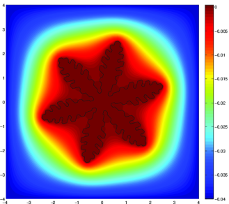
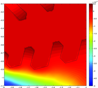
Figure 13. (One-sided Mullins–Sekerka problem) $\vec{X}(t)$ for for $t=0,\,5,\ldots,40$ (left). $\vec{X}(t)$ and $U(t)$ for $t=40$ on $[-4,4]^{2}$ (middle) and on $[-2,-1]\times[-1.1,-0.1]$ (right).

As a comparison, we repeat the same experiment as in Figure 13 now for (i) the one-sided Stefan problem, (ii) the two-sided Mullins–Sekerka problem, and (iii) the two-sided Stefan problem with $\vartheta=1$ for the Stefan problems. Note that for (ii) and (iii) we employ the finite-element approximation from [11], while for (i) we use (3.6a–c) with $\vartheta=1$. The corresponding plots are shown in Figures 14–16. We observe that the difference between the one-sided and the two-sided problems is not very pronounced, but one notices that the sidearms in the two-sided problems grow more slowly due to the fact that diffusion into the crystal is possible.

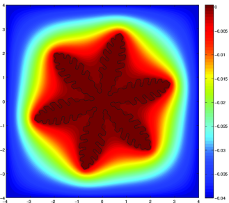
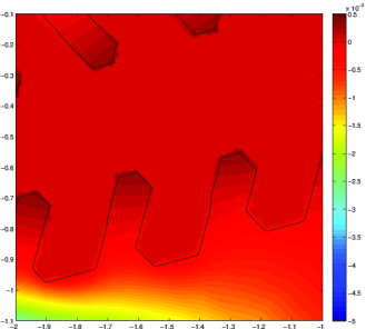
Figure 14. (One-sided Stefan problem) $\vec{X}(t)$ for for $t=0,\,5,\ldots,40$ (left). $\vec{X}(t)$ and $U(t)$ for $t=40$ on $[-4,4]^{2}$ (middle) and on $[-2,-1]\times[-1.1,-0.1]$ (right).

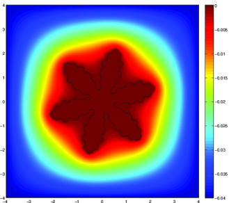
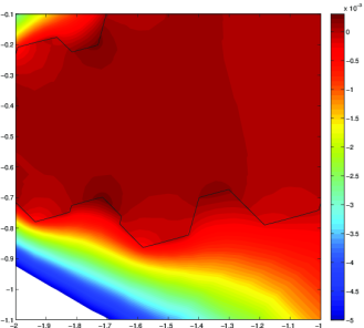
Figure 15. (Two-sided Mullins–Sekerka problem) $\vec{X}(t)$ for for $t=0,\,5,\ldots,40$ (left). $\vec{X}(t)$ and $U(t)$ for $t=40$ on $[-4,4]^{2}$ (middle) and on $[-2,-1]\times[-1.1,-0.1]$ (right).

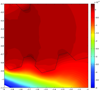
Figure 16. (Two-sided Stefan problem) $\vec{X}(t)$ for for $t=0,\,5,\ldots,40$ (left). $\vec{X}(t)$ and $U(t)$ for $t=40$ on $[-4,4]^{2}$ (middle) and on $[-2,-1]\times[-1.1,-0.1]$ (right).

In the final experiments for $d=2$, we return to the one-sided Mullins–Sekerka problem and set $u_{D}=-0.08$ and $u_{D}=-0.2$. The results are shown in Figures 17 and 18, respectively.

 

Figure 17. ($\Omega=(-4,4)^{2}$, $u_{D}=-0.08$, $\gamma=\beta$) $\vec{X}(t)$ for $t=0,\,0.2,\ldots,2$ (left), and for $t=0,\,2,\ldots,20$ (right). Parameters are $N_{f}=1024$, $N_{c}=K^{0}_{\Gamma}=64$, and $\tau=10^{-3}$.

 

Figure 18. ($\Omega=(-4,4)^{2}$, $u_{D}=-0.2$, $\gamma=\beta$) $\vec{X}(t)$ for $t=0,\,0.04,\ldots,0.4$ (left), and for $t=0,\,0.4,\ldots,6.4$ (right). Parameters are $N_{f}=2048$, $N_{c}=K^{0}_{\Gamma}=128$, and $\tau=2.5\times 10^{-4}$.

5.4. Crystal growth simulations for $d=3$

Throughout this subsection, unless otherwise stated, we use the parameters in (5.2) and $\gamma=\gamma_{hex}$ defined by (1.10) with $\varepsilon=0.01$ and $\theta_{0}=\frac{\pi}{12}$. Once again, we use this rotation of the anisotropy $\gamma$, so that the dominant growth directions are not exactly aligned with the $x_{1}$- and $x_{2}$-directions of the underlying finite-element meshes $\mathcal{T}^{m}$. Moreover, the radius of the initial crystal seed $\Gamma(0)$ is always chosen to be $R_{0}=0.05$. For later use, we define the kinetic coefficients

$$\beta_{\rm flat}(\vec{p})=\beta_{\rm flat,\ell}(\vec{p}):=[p_{1}^{2}+p_{2}^{2}+10^{-2\ell}\,p_{3}^{2}]^{\frac{1}{2}}\quad\text{with}\quad\ell\in\mathbb{N},$$ (5.5a)

and

$$\beta_{\rm tall}(\vec{p})=\beta_{\rm tall,\ell}(\vec{p}):=[10^{-2\ell}\,(p_{1}^{2}+p_{2}^{2})+p_{3}^{2}]^{\frac{1}{2}}\quad\text{with}\quad\ell\in\mathbb{N}.$$ (5.5b)

We note that in practice, similarly to the two-dimensional results in Figures 7 and 8, there was hardly any difference between the numerical results for a kinetic coefficient $\beta$ that is isotropic in the $x_{1}$-$x_{2}$ plane, such as $\beta_{\rm flat}$ and $\beta_{\rm tall}$, and one that is anisotropically aligned to the surface energy density, such as e.g. $\beta=\beta_{\rm flat}\,\gamma$. Hence in all our experiments we always choose coefficients $\beta$ that are isotropic in the $x_{1}$-$x_{2}$ plane, e.g. (5.5a,b).

In the first experiment, we set $u_{D}=-0.004$ and compare the results for the two coefficients $\beta=1$ and $\beta=\beta_{\rm flat,3}$; see Figures 19 and 20. We observe that the kinetic coefficient seems to be responsible for the fact whether solid prisms or thin plates grow; see also the Nakaya diagram in Figure 5 and [33]. More details of the evolution for the simulation in Figure 20 are given in Figure 21.

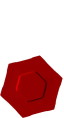
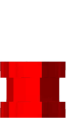
Figure 19. ($\Omega=(-4,4)^{3}$, $u_{D}=-0.004$, $\beta=1$) $\vec{X}(T)$ for $T=50$. Parameters are $N_{f}=128$, $N_{c}=16$, $K^{0}_{\Gamma}=98$, and $\tau=10^{-1}$.

Figure 20. ($\Omega=(-4,4)^{3}$, $u_{D}=-0.004$, $\beta=\beta_{\rm flat,3}$) $\vec{X}(T)$ for $T=50$. Parameters are $N_{f}=128$, $N_{c}=16$, $K^{0}_{\Gamma}=98$, and $\tau=10^{-1}$.

Figure 21. ($\Omega=(-4,4)^{3}$, $u_{D}=-0.004$, $\beta=\beta_{\rm flat,3}$) $\vec{X}(t)$ for $t=1,\,2,\,10,\,20,\,30,\,40,\,50$. Parameters are $N_{f}=128$, $N_{c}=16$, $K^{0}_{\Gamma}=98$, and $\tau=10^{-1}$.

A continuation of the evolution shown in Figure 21, now on the larger domain $\Omega=(-8,8)^{3}$, can be seen in Figure 22, where the onset of dendritic growth can be observed.

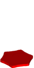
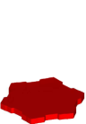
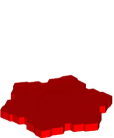
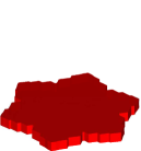
Figure 22. ($\Omega=(-8,8)^{3}$, $u_{D}=-0.004$, $\beta=\beta_{\rm flat,3}$) $\vec{X}(t)$ for $t=50,\,100,\,150,\,200$. Parameters are $N_{f}=256$, $N_{c}=32$, $K^{0}_{\Gamma}=98$, and $\tau=10^{-1}$.

An experiment for $u_{D}=-0.002$ and $\beta=\beta_{\rm tall,1}$ can be seen in Figure 23, where a solid prism grows.

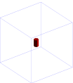
Figure 23. ($\Omega=(-4,4)^{3}$, $u_{D}=-0.002$, $\beta=\beta_{\rm tall,1}$) $\vec{X}(t)$ for $t=1,\,2,\,5,\,10,\,20,\,30,\,40,\,50$; and $\vec{X}(50)$ within $\Omega$. Parameters are $N_{f}=128$, $N_{c}=16$, $K^{0}_{\Gamma}=98$, and $\tau=10^{-1}$.

An experiment for $u_{D}=-0.008$ and $\beta=\beta_{\rm tall,2}$ can be seen in Figure 24. In this case the basal facets break, leading to hollow columns; see Figure 5 and [26].

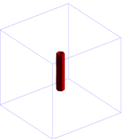
Figure 24. ($\Omega=(-4,4)^{3}$, $u_{D}=-0.008$, $\beta=\beta_{\rm tall,2}$) $\vec{X}(t)$ for $t=1,\,2,\,5,\,10,\,20,\,30,\,40,\,50$; and $\vec{X}(50)$ within $\Omega$. Parameters are $N_{f}=128$, $N_{c}=16$, $K^{0}_{\Gamma}=98$, and $\tau=10^{-1}$.

An experiment for $u_{D}=-0.02$ and $\beta=\beta_{\rm flat,3}$ can be seen in Figure 25. In this case the prism facets break, leading to capped columns which also can be observed in nature; see [33].

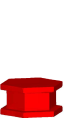
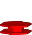
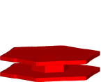
Figure 25. ($\Omega=(-4,4)^{3}$, $u_{D}=-0.02$, $\beta=\beta_{\rm flat,3}$) $\vec{X}(t)$ for $t=0.05,\,0.1,\,0.2,\,0.3$; and $\vec{X}(0.3)$ within $\Omega$. Parameters are $N_{f}=512$, $N_{c}=32$, $K^{0}_{\Gamma}=1538$ and $\tau=5\times 10^{-4}$.

An experiment for $u_{D}=-0.02$ and $\beta=\beta_{\rm flat,3}$, but for the anisotropy $\gamma$ defined by

$$\gamma(\vec{p})=2\,l_{\varepsilon}(R_{2}(\tfrac{\pi}{2})\,\vec{p})+\sum_{\ell=1}^{3}l_{\varepsilon}(R_{1}(\theta_{0}+\tfrac{\ell\,\pi}{3})\,\vec{p}).$$ (5.6)

with $\varepsilon=0.01$ and $\theta_{0}=\frac{\pi}{12}$ can be seen in Figure 26. This leads to a geometrically more complicated breaking of the prismal facets. These can also be observed in nature, and they are called hollow plates; see [33].

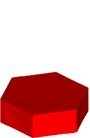
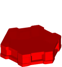
Figure 26. ($\Omega=(-4,4)^{3}$, $u_{D}=-0.02$, $\gamma$ as in (5.6), $\beta=\beta_{\rm flat,3}$) $\vec{X}(t)$ for $t=0.5,\,1$. Parameters are $N_{f}=512$, $N_{c}=32$, $K^{0}_{\Gamma}=98$, and $\tau=10^{-3}$.

We also performed simulations varying $\beta$ in time. This is realistic as a growing snow crystal falls to the earth through changing weather conditions, which influence the governing parameters, e.g. via the temperature. In the first such example, we choose

$$\beta(\vec{p})=\begin{cases}\beta_{\rm flat,3}(\vec{p})&t\in[0,30),\\ \beta_{\rm tall,3}(\vec{p})&t\in[30,\infty).\end{cases}$$ (5.7a)

In a second example we choose

$$\beta(\vec{p})=\begin{cases}\beta_{\rm flat,3}(\vec{p})&t\in[0,20),\\ \beta_{\rm flat,1}(\vec{p})&t\in[20,\infty).\end{cases}$$ (5.7b)

Results for these choices of $\beta$ and for $u_{D}=-0.004$ can be seen in Figure 27. The shapes in Figure 27 can also be observed in nature, and they are called scrolls on plates.

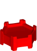
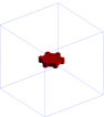
Figure 27. ($\Omega=(-4,4)^{3}$, $u_{D}=-0.004$, $\beta$ as in (5.7a,b)) $\vec{X}(T)$ for $T=50$. Parameters are $N_{f}=128$, $N_{c}=16$, $K^{0}_{\Gamma}=98$, and $\tau=10^{-1}$.

The remaining numerical experiments are for the cylindrical anisotropy (1.11) with $\varepsilon=10^{-2}$; recall Figure 4. The first case is for $\gamma_{\rm TB}=1$, $u_{D}=-0.004$, and $\beta=\beta_{\rm tall,1}$, and the results, which show facet breaking both in the basal and prismal directions, can be seen in Figure 28. Some plots of the concentration are shown in Figures 29 and 30, where

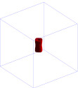
Figure 28. ($\Omega=(-4,4)^{3}$, $u_{D}=-0.004$, $\beta=\beta_{\rm tall,1}$) $\vec{X}(t)$ for $t=1,\,2,\,5,\,10,\,20,\,30,\,40,\,50$; and $\vec{X}(50)$ within $\Omega$. Parameters are $N_{f}=128$, $N_{c}=16$, $K^{0}_{\Gamma}=98$, and $\tau=10^{-1}$.

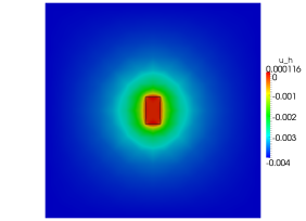
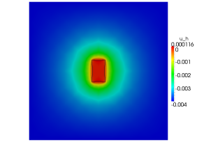
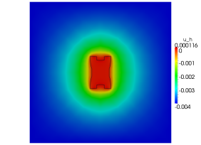
Figure 29. ($\Omega=(-4,4)^{3}$, $u_{D}=-0.004$, $\beta=\beta_{\rm tall,1}$) $\vec{X}(t)\cap\{\vec{z}:z_{1}=0\}$ and $U(t)\!\mid_{z_{1}=0}$ for $t=15,\,25,\,50$. Parameters are $N_{f}=128$, $N_{c}=16$, $K^{0}_{\Gamma}=98$, and $\tau=10^{-1}$.

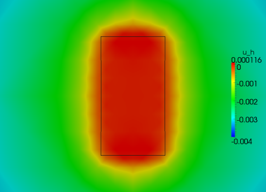
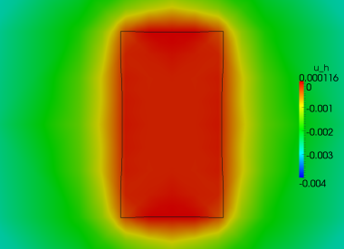
Figure 30. ($\Omega=(-4,4)^{3}$, $u_{D}=-0.004$, $\beta=\beta_{\rm tall,1}$) $\vec{X}(t)\cap\{\vec{z}:z_{1}=0\}$ and $U(t)\!\mid_{z_{1}=0}$ for $t=10,\,15$. Parameters are $N_{f}=128$, $N_{c}=16$, $K^{0}_{\Gamma}=98$, and $\tau=10^{-1}$.

Berg’s effect (see e.g. [24]) can clearly be seen; i.e., $U$ increases towards the centre of the basal face before facet breaking occurs.

For the anisotropy (1.11) it is of interest to find for what value of $\gamma_{\rm TB}$ the evolution of (1.1a–e) with

$$\vartheta=0,\quad\mathcal{K}=1,\quad\lambda=1,\quad\rho=1,\quad\alpha=1,\quad a=1,\quad\beta=\gamma,\quad f=0$$ (5.8)

is self-similar. For example, in [25] it was shown that there exists a value $\gamma_{\rm TB}>0$ for which this is the case. Numerically this can be checked by starting this flow with a scaled Wulff shape (or a shape close to that), and then to observe whether the height-to-basal-diameter ratio of the evolving approximate cylinder converges to $\gamma_{\rm TB}$.

In practice we choose $\Gamma(0)$ to be a cylinder with basal radius $R_{0}=0.1$ and a height/basal diameter ratio of $\gamma_{\rm TB}$. In order to obtain the desired sign for $\mathcal{V}$, i.e., for an expanding evolution, we set $u_{D}=-21$ in (1.1d). For the domain $\Omega$ we choose $\Omega=(-8,8)^{3}$.

In practice we appear to obtain a value for self-similarity for some $\gamma_{\rm TB}\in[0.92,0.93]$, although the precise value seems to depend on the resolution of the bulk mesh. In Figure 31 we plot some results for an experiment with $\gamma_{\rm TB}=0.925$, while in Figure 32 we show the evolution of the ratio of interest for two experiments with $\gamma_{\rm TB}=0.92$ and $\gamma_{\rm TB}=0.925$, respectively. These results seem to indicate that there exists a value $\gamma_{\rm TB}$ close to $\gamma_{\rm TB}=0.92$ for which the evolution of (1.1a–e) with (5.8) and (1.11) is self-similar.

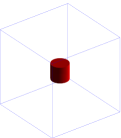
Figure 31. ($\Omega=(-8,8)^{3}$, $\gamma_{\rm TB}=0.925$) $\vec{X}(t)$ for $t=0,\,0.1,\,0.2$; and $\vec{X}(0.2)$ within $\Omega$. Parameters are $N_{f}=512$, $N_{c}=32$, $K^{m}_{\Gamma}\equiv 1538$, and $\tau=10^{-4}$.

Figure 32. Plots of the height/basal diameter ratio for the two runs with $\gamma_{\rm TB}=0.92$ (top) and $\gamma_{\rm TB}=0.925$ (bottom). The dashed lines show the value of $\gamma_{\rm TB}$.

Conclusions

We have presented a fully practical finite-element approximation for one-sided Mullins–Sekerka and Stefan problems with anisotropic Gibbs–Thomson law and kinetic undercooling. In particular, the method allows the approximation of a continuum model for snow crystal growth, which is based on rigorous thermodynamical principles and balance laws. To our knowledge, the numerical results presented in this paper are the first simulations of snow crystal growth that are based on such a rigorous, physically motivated model.

In our numerical simulations of snow crystal growth in three space dimensions, we were able to produce a significant number of different types of snow crystals. In particular (recall Figure 5), we obtained results that resemble solid plates, solid prisms, hollow columns, dendrites, capped columns, and scrolls on plates. Also, facet breaking in the moving-boundary problems computed have been observed in cases with nearly crystalline anisotropic energies; see also [26] for theoretical predictions of facet breaking. We therefore believe that the results presented here may help to understand the different factors that play a role in the shaping of snow crystals in the real world.

Producing more complicated dendritic shapes in three space dimensions, with complicated substructures such as steps and ridges, as in e.g. [33, Figure 1], or as in the beautiful simulations in [30], which were obtained with a cellular automata algorithm, would need a much higher computational cost when computed with the help of a discretized moving-boundary problem for a diffusion equation. The main reason is that the highly detailed and irregularly structured surface of snow flakes (see e.g. Figure 1(c) in [33]) would need to be accurately captured with a triangulated surface $\Gamma^{m}$, say. On this surface, a second-order partial differential equation then needs to be solved, which is coupled to a PDE in the bulk. The necessary resolutions for both meshes, as well as the involved computational effort to solve the linear systems arising from (3.6a–c), mean that on currently available computer hardware those kind of computations cannot be performed.

Nevertheless, it is our belief that the numerical methods presented here, combined with suitable randomizations and fluctuations of physical parameters together with sophisticated computing equipment, should be able to produce all the possible variations of realistic snow crystals. In addition, we believe that the computations presented in this paper are the most accurate and complex which have been computed so far with the help of a Stefan or Mullins–Sekerka problem with hexagonal symmetry.

Acknowledgment. We are grateful to Prof. Libbrecht for allowing us to use Figure 5.

References

- [1] P.R. Amestoy, T.A. Davis, and I.S. Duff, Algorithm 837: AMD, an approximate minimum degree ordering algorithm, ACM Trans. Math. Software, 30 (2004), 381–388.
- [2] L’. Baňas and R. Nürnberg, Finite element approximation of a three dimensional phase field model for void electromigration, J. Sci. Comp., 37 (2008), 202–232.
- [3] E. Bänsch and A. Schmidt, Simulation of dendritic crystal growth with thermal convection, Interfaces Free Bound., 2 (2000), 95–115.
- [4] J.W. Barrett and C.M. Elliott, A finite element method on a fixed mesh for the Stefan problem with convection in a saturated porous medium, in K.W. Morton and M.J. Baines, editors, “Numerical Methods for Fluid Dynamics,” Academic Press (London), 1982, 389–409.
- [5] J.W. Barrett, H. Garcke, and R. Nürnberg, On the variational approximation of combined second and fourth order geometric evolution equations, SIAM J. Sci. Comput., 29 (2007), 1006–1041.
- [6] J.W. Barrett, H. Garcke, and R. Nürnberg, A parametric finite element method for fourth order geometric evolution equations, J. Comput. Phys., 222 (2007), 441–462.
- [7] J.W. Barrett, H. Garcke, and R. Nürnberg, Numerical approximation of anisotropic geometric evolution equations in the plane, IMA J. Numer. Anal., 28 (2008), 292–330.
- [8] J.W. Barrett, H. Garcke, and R. Nürnberg, On the parametric finite element approximation of evolving hypersurfaces in , J. Comput. Phys., 227 (2008), 4281–4307.
- [9] J.W. Barrett, H. Garcke, and R. Nürnberg, A variational formulation of anisotropic geometric evolution equations in higher dimensions, Numer. Math., 109 (2008), 1–44.
- [10] J.W. Barrett, H. Garcke, and R. Nürnberg, Finite element approximation of coupled surface and grain boundary motion with applications to thermal grooving and sintering, European J. Appl. Math., 21 (2010), 519–556.
- [11] J.W. Barrett, H. Garcke, and R. Nürnberg, On stable parametric finite element methods for the Stefan problem and the Mullins–Sekerka problem with applications to dendritic growth, J. Comput. Phys., 229 (2010), 6270–6299.
- [12] J.W. Barrett, H. Garcke, and R. Nürnberg, Parametric approximation of surface clusters driven by isotropic and anisotropic surface energies, Interfaces Free Bound., 12 (2010), 187–234.
- [13] J.W. Barrett, H. Garcke, and R. Nürnberg, Numerical computations of faceted pattern formation in snow crystal growth, Phys. Rev. E, 86 (2012), 011604.
- [14] J.W. Barrett, R. Nürnberg, and V. Styles, Finite element approximation of a phase field model for void electromigration, SIAM J. Numer. Anal., 42 (2004), 738–772.
- [15] G. Bellettini, M. Novaga, and M. Paolini, Facet-breaking for three-dimensional crystals evolving by mean curvature, Interfaces Free Bound., 1 (1999), 39–55.
- [16] S.H. Davis, “Theory of Solidification,” Cambridge Monographs on Mechanics, Cambridge University Press, Cambridge, 2001.
- [17] T.A. Davis, Algorithm 849: a concise sparse Cholesky factorization package, ACM Trans. Math. Software, 31 (2005), 587–591.
- [18] K. Deckelnick, G. Dziuk, and C.M. Elliott, Computation of geometric partial differential equations and mean curvature flow, Acta Numer., 14 (2005), 139–232.
- [19] G. Dziuk, An algorithm for evolutionary surfaces, Numer. Math., 58 (1991), 603–611.
- [20] I. Fonseca and S. Müller, A uniqueness proof for the Wulff theorem, Proc. Roy. Soc. Edinburgh Sect. A, 119 (1991), 125–136.
- [21] H. Garcke and S. Schaubeck, Existence of weak solutions for the Stefan problem with anisotropic Gibbs–Thomson law, Adv. Math. Sci. Appl., 21 (2011), 255–283.
- [22] M.-H. Giga and Y. Giga, A subdifferential interpretation of crystalline motion under nonuniform driving force, Discrete Contin. Dynam. Systems, pp. 276–287, “Dynamical Systems and Differential Equations, Vol. I,” Springfield, MO, 1996.
- [23] Y. Giga, “Surface Evolution Equations,” Birkhäuser, Basel, 2006.
- [24] Y. Giga and P. Rybka, Berg’s effect, Adv. Math. Sci. Appl., 13 (2003), 625–637.
- [25] Y. Giga and P. Rybka, Existence of self-similar evolution of crystals grown from supersaturated vapor, Interfaces Free Bound., 6 (2004), 405–421.
- [26] Y. Giga and P. Rybka, Stability of facets of crystals growing from vapor, Discrete Contin. Dyn. Syst., 14 (2006), 689–706.
- [27] T. Gonda and T. Yamazaki, Morphological stability of polyhedral ice crystals growing from the vapor phase, J. Cryst. Growth, 60 (1982), 259–263.
- [28] P. Górka, Evolution of 3-D crystals from supersaturated vapor with modified Stefan condition: Galerkin method approach, J. Math. Anal. Appl., 341 (2008), 1413–1426.
- [29] P. Górka, Quasi-static evolution of polyhedral crystals, Discrete Contin. Dyn. Syst. Ser. B, 9 (2008), 309–320.
- [30] J. Gravner and D. Griffeath, Modeling snow-crystal growth: A three-dimensional mesoscopic approach, Phys. Rev. E, 79 (2009), 011601.
- [31] M.E. Gurtin, “Thermomechanics of Evolving Phase Boundaries in the Plane,” Oxford Mathematical Monographs, The Clarendon Press Oxford University Press, New York, 1993.
- [32] R. Kobayashi and Y. Giga, On anisotropy and curvature effects for growing crystals, Japan J. Indust. Appl. Math., 18 (2001), 207–230.
- [33] K.G. Libbrecht, The physics of snow crystals, Rep. Progr. Phys., 68 (2005), 855–895.
- [34] S. Luckhaus, Solutions for the two-phase Stefan problem with the Gibbs–Thomson law for the melting temperature, European J. Appl. Math., 1 (1990), 101–111.
- [35] H.R. Pruppacher and J.D. Klett, “Microphysics of Clouds and Precipitation,” Kluwer Acad. Publ., Dordrecht, 1997.
- [36] A. Schmidt, “Die Berechnung dreidimensionaler Dendriten mit Finiten Elementen,” Ph.D. thesis, University Freiburg, Freiburg, 1993.
- [37] A. Schmidt, Computation of three dimensional dendrites with finite elements, J. Comput. Phys., 195 (1996), 293–312.
- [38] A. Schmidt, Approximation of crystalline dendrite growth in two space dimensions, in J. Kačur and K. Mikula, editors, Proceedings of the Algoritmy ’97 Conference on Scientific Computing (Zuberec), volume 67, Slovak University of Technology, Bratislava (1998), pages 57–68.
- [39] A. Schmidt and K.G. Siebert, “Design of Adaptive Finite Element Software: The Finite Element Toolbox ALBERTA,” volume 42 of Lecture Notes in Computational Science and Engineering, Springer-Verlag, Berlin, 2005.
- [40] G. Wulff, Zur Frage der Geschwindigkeit des Wachstums und der Auflösung der Kristallflächen, Z. Krist., 34 (1901), 449–530.
- [41] E. Yokoyama, Formation of patterns during growth of snow crystals, J. Cryst. Growth, 128 (1993), 251–257.
- [42] E. Yokoyama and R.F. Sekerka, A numerical study of the combined effect of anisotropic surface tension and interface kinetics on pattern formation during the growth of two-dimensional crystals, J. Cryst. Growth, 125 (1992), 389–403.