Femtosecond two-photon photoassociation of hot magnesium atoms:
A quantum dynamical study using thermal random phase wavefunctions

Abstract

Two-photon photoassociation of hot magnesium atoms by femtosecond laser pulses, creating electronically excited magnesium dimer molecules, is studied from first principles, combining ab initio quantum chemistry and molecular quantum dynamics. This theoretical framework allows for rationalizing the generation of molecular rovibrational coherence from thermally hot atoms [L. Rybak et al., Phys. Rev. Lett. 107, 273001 (2011)]. Random phase thermal wave functions are employed to model the thermal ensemble of hot colliding atoms. Comparing two different choices of basis functions, random phase wavefunctions built from eigenstates are found to have the fastest convergence for the photoassociation yield. The interaction of the colliding atoms with a femtosecond laser pulse is modeled non-perturbatively to account for strong-field effects.

I Introduction

Molecules can be assembled from atoms using laser light. This process is termed photoassociation. With the advent of femtosecond lasers and pulse shaping techniques, photoassociation became a natural candidate for coherent control of a binary reaction. Coherent control had been conceived as a method to determine the fate of chemical reactions using laser fields.RonnieDancing89 The basic idea is to employ interference of matter waves to constructively enhance a desired outcome while destructively suppressing all undesired alternatives.RiceBook ; ShapiroBook Control is exerted by shaping the laser pulses, the simplest control knobs being time delays and phase differences.DavidBook Over the last two decades, the field of coherent control has developed significantly both theoretically and experimentally.GordonARPC97 ; BrixnerCPC03 ; DantusCR04 ; WollenhauptARPC05 ; SFB450book However, a critical examination of the achievements reveals that successful control has been demonstrated almost exclusively for unimolecular processes such as ionization, dissociation and fragmentation. It is natural to ask why the reverse process of controlling binary reactionsMarvetCPL95 ; BackhausCP97 ; GrossJCP97 ; BackhausJPCA98 ; BackhausCPL99 ; ReginaFaraday99 ; BonnSci99 ; GeppertJCP03 ; NuernbergerPNAS10 is so much more difficult.

The main difference between unimolecular processes and a binary reaction lies in the initial state – a single or few well-defined bound quantum states vs an incoherent continuum of scattering states.ZemanPRL04 For a binary reaction, the nature of the scattering continuum is mainly determined by the temperature of the reactants. As temperature decreases, higher partial waves are frozen out. At the very low temperatures of ultracold gases, the scattering energy of atom pairs is so low that the rotational barrier cannot be passed, and the scattering becomes purely $s$-wave.photoasso In this regime, the reactants are pre-correlated due to quantum threshold effectsMyPRL09 and the effect of scattering resonances is particularly pronounced.PellegriniPRL08 ; AlyabyshevPRA10 ; GonzalezKochPRA12 At a temperature of about 100$\,\mu$K, photoassociation with femtosecond laser pulses has been demonstrated.SalzmannPRL08 Coherent transient Rabi oscillations were observed as the prominent feature in the pump-probe spectra. The transients are due to long tails of the pulses caused by a sharp spectral cut which is necessary to avoid excitation into unbound states.SalzmannPRL08 ; MerliMyPRA09 This pinpoints to the fact that the large spectral bandwidth of a femtosecond pulse is unsuitable to one-photon photoassociation at ultralow temperatures. In this regime, a narrow-band transition needs to be driven in order to avoid atomic excitation.MyPRA06a ; MyFaraday09 ; TomzaKochPRA12

The situation changes completely for high temperatures where the scattering states can penetrate rotational barriers due to the large translational kinetic energy. The association process is then likely to happen at short internuclear distance close to the inner turning point and for highly excited rotational states. In this case, the large spectral bandwidth of femtosecond laser pulses is ideally adapted to both the broad thermal width of the ensemble of scattering states and the depth of the electronically excited state potential in which molecules are formed. The disadvantage of this setting is that the initial state is completely incoherent, impeding control of the photoreaction. Photoassociation with femtosecond laser pulses was first demonstrated under these conditions, employing a one-photon transition in the UV.MarvetCPL95 Subsequent to the photoassociation, coherent rotational motion of the molecules was observed.MarvetCPL95 We have recently demonstrated generation of both rotational and vibrational coherences by two-photon femtosecond photoassociation of hot atoms.RybakPRL11 ; RybakFaraday This is a crucial step toward the coherent control of photoinduced binary reactions since the fate of bond making and breaking is determined by the vibrational motion.

Employing multi-photon transitions comes with several advantages: The class of molecules that can be photoassociated by near-IR/visible femtosecond laser pulses is significantly larger for multi-photon than one-photon excitation. Femtosecond laser technology is most advanced in the near-IR spectral region. Due to the different selection rules, different electronic states become accessible for multi-photon transitions compared to one-photon excitation. Control strategies differ for multi-photon and one-photon excitation. In particular, large dynamic Stark shifts and an extended manifold of quantum pathways that can be interfered come into play for multi-photon excitation.YaronARPC09 The theoretical description needs to account for these strong-field effects.

We have constructed a comprehensive theoretical model from first principles to describe the experiment in which magnesium atoms in a heated cell are photoassociated by femtosecond laser pulses.RybakPRL11 ; RybakFaraday It is summarized in Figure 1.

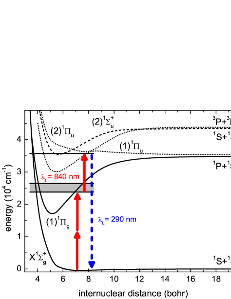
Figure 1: Potential energy curves of the electronic states involved in the two-photon photoassociation probed by a time-delayed pulse. The shaded region indicates the vibrational band populated after photoassociation.

Magnesium in its electronic ground state is a closed shell atom. Its ground electronic potential, X${}^{1}\Sigma_{g}^{+}$, therefore displays only a weak van der Waals attractive well. A femtosecond pulse of 100 fs transform-limited duration with a central wavelength of $\sim 840\,$nm promotes an electron to the $\pi$ orbital. This two-photon transition is driven since a wavelength of 840 nm is far from any one-photon resonance both for magnesium atoms and Mg₂ molecules, cf. Fig. 1. Upon excitation, a strong chemical bond is formed in the $(1)^{1}\Pi_{g}$ state with a binding energy of $\sim 1.8\,$eV or, equivalently, $\sim 14500\,$cm^-1. A time-delayed femtosecond pulse probes the excited Mg₂ molecule by inducing a one-photon transition to a higher excited electronic state (${}^{1}\Pi_{u}$). This state has a strong one-photon transition back to the ground state. The corresponding experimental observable is the intensity of the resulting UV fluorescence ($\sim 290\,$nm), measured as a function of the pump-probe time delay. An oscillating signal is a manifestation of coherent rovibrational dynamics in the ${}^{1}\Pi_{g}$ state.RybakPRL11 ; RybakFaraday

The correct description of the thermal initial state is crucial to capture the generation of coherence out of an incoherent ensemble. The density operator, $\boldsymbol{\mathsf{\hat{\rho}}}_{T}$, describing the initial state of hot atom pairs at temperature, $T$, is constructed by a thermal average over suitable basis functions. Since no dissipative processes occur on the sub-picosecond timescale of the experiment, the coherent time evolution of the density operator is efficiently carried out by propagating the basis functions. Expectation values are obtained by thermally averaging the corresponding operator over the propagated basis functions. A numerically efficient description of the initial thermal ensemble is essential to facilitate the time-dependent simulations. The present work on ab initio simulation of ultrafast hot photoassociation presents a detailed account of theoretical and numerical components and their integration into a comprehensive framework.

The paper is organized as follows. Section II presents the theoretical framework by introducing the Hamiltonian describing the coherent interaction of an atom pair with strong femtosecond laser pulses. The relevant electronic states, their potential energy curves, transition matrix elements and non-adiabatic couplings, all obtained employing highly accurate state of the art ab initio methods, are discussed. Section III derives an effective description of the thermal ensemble of translationally and rotationally hot atom pairs in their electronic ground state based on random phase thermal wave functions. We consider three different choices of basis functions, two of them turn out to be practical. Convergence of the photoassociation probability is studied in Section IV for the different thermal averaging procedures, and the role of shape resonances is discussed. Section V investigates the generation of coherence in terms of the quantum purity and a dynamical coherence measure. Finally, we conclude in Section VI. Atomic units are used throughout our paper, unless specified otherwise.

II ab initio Model

The coherent (2+1) three-photon excitation of a pair of magnesium atoms, that collide with rotational quantum number $J$, by a strong femtosecond laser pulse is described by the time-dependent Hamiltonian,

$$\boldsymbol{\mathsf{\hat{H}}}^{J}(t)=\begin{pmatrix}\boldsymbol{\mathsf{\hat{H}}}^{J}_{X^{1}\Sigma_{g}^{+}}+\omega^{S}_{X^{1}\Sigma_{g}^{+}}(t,R)&\chi^{\star}(t,R)&0&0&0&0\\ \chi(t,R)&\boldsymbol{\mathsf{\hat{H}}}^{J}_{(1)^{1}\Pi_{g}}+\omega^{S}_{(1)^{1}\Pi_{g}}(t,R)&W_{1}(R)&W_{2}(R)&\mu_{1}(R)E^{\star}(t)&\mu_{2}(R)E^{\star}(t)\\ 0&W_{1}(R)&\boldsymbol{\mathsf{\hat{H}}}^{J}_{(1)^{3}\Sigma^{+}_{g}}&W_{3}(R)&0&0\\ 0&W_{2}(R)&W_{3}(R)&\boldsymbol{\mathsf{\hat{H}}}^{J}_{(1)^{3}\Pi_{g}}&0&0\\ 0&\mu_{1}(R)E(t)&0&0&\boldsymbol{\mathsf{\hat{H}}}_{11}^{J}+\omega^{S}_{11}(t,R)&V_{12}(R)+\omega^{S}_{12}(t,R)\\ 0&\mu_{2}(R)E(t)&0&0&V_{12}(R)+\omega^{S}_{12}(t,R)&\boldsymbol{\mathsf{\hat{H}}}_{22}^{J}+\omega^{S}_{22}(t,R)\\ \end{pmatrix}\,.$$ (1)

Here $\boldsymbol{\mathsf{\hat{H}}}^{J}_{a}$ is the nuclear Hamiltonian of electronic state $a$,

$$\boldsymbol{\mathsf{\hat{H}}}^{J}_{a}=\boldsymbol{\mathsf{\hat{T}}}+V_{a}(R)+\frac{J(J+1)}{2mR^{2}}\,,$$ (2)

with $\boldsymbol{\mathsf{\hat{T}}}=\boldsymbol{\mathsf{\hat{P}}}^{2}/2m$ the vibrational kinetic energy, $m$ the reduced mass and $V_{a}(R)$ the potential energy curve of electronic state $a$. $\mu_{1}$ and $\mu_{2}$ denote the (one-photon) transition dipole moments between the $(1)^{1}\Pi_{g}$ state and the first and second ${}^{1}\Pi_{u}$ states. The Hamiltonian (1) neglects ro-vibrational couplings. In a two-photon rotating-wave approximation, the two-photon coupling between the $X^{1}\Sigma_{g}^{+}$ $(g)$ and $(1)^{1}\Pi_{g}$ $(e)$ states is denoted by $\chi(t,R)$,BoninBook

$$\chi(t,R)=\frac{1}{4}E(t)^{2}\sum_{i,j}\epsilon_{i}\epsilon_{j}M_{ij}^{e\leftarrow g}(R),$$ (3)

with $E(t)=S(t)e^{i\varphi(t)}$ the electric field envelope of the laser pulse, $\epsilon_{i}$ the polarization component ($i=\perp,\parallel$), and $M_{ij}^{e\leftarrow g}$ the tensor elements of the two-photon electric transition dipole moment between the ground ($g$) and excited ($e$) states,BoninBook

$$M_{ij}^{e\leftarrow g}(R)=-\sum_{n}\left[\frac{\langle e|\boldsymbol{\mathsf{\hat{\mu}}}_{i}|n\rangle\langle n|\boldsymbol{\mathsf{\hat{\mu}}}_{j}|g\rangle}{\omega_{ng}-\omega_{L}}+\frac{\langle e|\boldsymbol{\mathsf{\hat{\mu}}}_{j}|n\rangle\langle n|\boldsymbol{\mathsf{\hat{\mu}}}_{i}|g\rangle}{\omega_{ne}+\omega_{L}}\right]\,.$$ (4)

The summation is carried out over all electronic states $n$, except for the states which are explicitly accounted for in our model, cf. Eq. (1). $\omega_{ng}$ and $\omega_{ne}$ are the transition frequencies between state $n$ and, respectively, state $g=X^{1}\Sigma_{g}$ and $e=^{1}\Pi_{g}$. Note that the two-photon transition moment, $M_{ij}^{e\leftarrow g}(R)$, depends on the central laser frequency, $\omega_{L}=hc/\lambda_{L}$. Here we keep $\lambda_{L}=840\,$nm fixed. The strong laser field driving the two-photon transitions may lead to non-negligible dynamic Stark shifts $\omega^{S}_{a}(t,R)$,BoninBook

$$\omega^{S}_{a}(t,R)=-\frac{1}{4}|E(t)|^{2}\sum_{i,j}\epsilon_{i}\epsilon_{j}\alpha^{a}_{ij}(\omega_{L},R)\,,$$ (5)

where the tensor elements of the dynamic electric dipole polarizability are given byBoninBook

$$\alpha^{a}_{ij}(R)=\sum_{n\neq a}\left[\frac{\langle a|\boldsymbol{\mathsf{\hat{\mu}}}_{i}|n\rangle\langle n|\boldsymbol{\mathsf{\hat{\mu}}}_{j}|a\rangle}{\omega_{na}-\omega_{L}}+\frac{\langle a|\boldsymbol{\mathsf{\hat{\mu}}}_{j}|n\rangle\langle n|\boldsymbol{\mathsf{\hat{\mu}}}_{i}|a\rangle}{\omega_{na}+\omega_{L}}\right]\,,$$ (6)

where the sum runs over all electronic states $n$, except those explicitly accounted for in our model, cf. Eq. (1), and $\omega_{na}$ is the transition frequency between states $n$ and $a$ ($a=e,g$). We account only for the isotropic part of the polarizability, neglecting anisotropic terms that occur for open shell states with the projection of the electronic angular momentum not equal to zero.SkomorowskiJCP11 ; TomzaMolPhys13 This corresponds to two-photon transitions with $\Delta J=0$, neglecting transitions with $\Delta J=\pm 2$. Similarly to the two-photon transition moment, $M_{ij}^{e\leftarrow g}(R)$, the dynamic polarizability, $\alpha^{a}_{ij}(R)$, depends on the central laser frequency, $\omega_{L}$. Note that resonant transitions, both one-photon and two-photon transitions, are treated in a non-perturbative way while all non-resonant transitions are accounted for within second order perturbation theory.

The $(1)^{1}\Pi_{g}$ excited state that is accessed by the two-photon transition is weakly coupled to the $(1)^{3}\Pi_{g}$, and $(1)^{3}\Sigma_{g}$ states due to the spin-orbit interaction. The spin-orbit matrix elements relevant for our work read

$$W_{1}(R)=\langle\Psi_{(1)^{1}\Pi_{g}}|H_{\rm SO}|\Psi_{(1)^{3}\Sigma_{g}}\rangle,$$ (7)

$$W_{2}(R)=\langle\Psi_{(1)^{1}\Pi_{g}}|H_{\rm SO}|\Psi_{(1)^{3}\Pi_{g}}\rangle,$$ (8)

$$W_{3}(R)=\langle\Psi_{(3)^{1}\Pi_{g}}|H_{\rm SO}|\Psi_{(1)^{3}\Sigma_{g}}\rangle,$$ (9)

where $H_{\rm SO}$ is the spin-orbit coupling Hamiltonian in the Breit-Pauli approximation including all one- and two-electron terms. The effect of the spin-orbit coupling was actually observed in the fluorescence signal, but it was so weak that we could neglect the triplet states in the time-dependent calculations. A one-photon transition connects the $(1)^{1}\Pi_{g}$ state to the adiabatic $(1)^{1}\Pi_{u}$ and $(2)^{1}\Pi_{u}$ states that are strongly coupled by the radial nuclear momentum operator. In order to include this non-adiabatic coupling, the diabatic representation is employed, see e.g. Ref. BaerBook, . $V_{11}^{\rm d}$ and $V_{22}^{\rm d}$ denote the corresponding diagonal diabatic potentials and $V_{12}(R)=V_{21}(R)$ the coupling term. Analogously, $\omega^{S}_{ij}(t,R)$ ($i,j=1,2$) denote the Stark shifts in the diabatic basis. The angle of the rotation matrix transforming adiabatic into diabatic representation is given byBaerBook

$$\zeta(R)=\int_{R}^{\infty}\tau(R^{\prime})dR^{\prime}$$ (10)

with the nonadiabatic radial coupling

$$\tau(R)=\left\langle\Psi_{(1)^{1}\Pi_{u}}\left|\frac{\mathrm{d}}{\mathrm{d}R}\right|\Psi_{(2)^{1}\Pi_{u}}\right\rangle\,.$$ (11)

Consequently, the one-photon transition dipole moments $\mu_{1}(R)$, $\mu_{2}(R)$ are calculated from the diabatic molecular wave functions, obtained by rotating the adiabatic $(1)^{1}\Pi_{u}$ and $(2)^{1}\Pi_{u}$ wave functions.

Table 1: Spectroscopic characteristics, i.e., equilibrium bond lengths, $R_{e}$, and well depths, $D_{e}$, of our ab initio potentials.

state	$R_{e}$ (bohr)	$D_{e}$ (cm-1)	Dissociation
$X^{1}\Sigma_{g}^{+}$	7.33	430	$(1)^{1}S+(1)^{1}S$
$(1)^{3}\Sigma_{g}^{+}$	12.80	49	$(1)^{1}S+(1)^{3}P$
$(1)^{3}\Pi_{g}$	5.31	7963	$(1)^{1}S+(1)^{3}P$
$(1)^{3}\Sigma_{u}^{+}$	5.72	7459	$(1)^{1}S+(1)^{3}P$
$(1)^{3}\Pi_{u}$	8.60	110	$(1)^{1}S+(1)^{3}P$
(2)${}^{1}\Sigma_{g}^{+}$	6.22	2221	$(1)^{1}S+(1)^{1}P$
(1)${}^{1}\Pi_{g}$	5.10	18077	$(1)^{1}S+(1)^{1}P$
A${}^{1}\Sigma_{u}^{+}$	5.75	9427	$(1)^{1}S+(1)^{1}P$
(1)${}^{1}\Pi_{u}$	5.50	5395	$(1)^{1}S+(1)^{1}P$
(3)${}^{1}\Sigma_{g}^{+}$	5.00	6203	$(1)^{1}S+(2)^{1}S$
(2)${}^{1}\Sigma_{u}^{+}$	5.57	8262	$(1)^{1}S+(2)^{1}S$

State-of-the-art ab initio techniques have been applied to compute the potential energy curves of the magnesium dimer in the Born-Oppenheimer approximation. All calculations employed the aug-cc-pVQZ basis set of quadruple zeta quality as the atomic basis for Mg. This basis set was augmented by the set of bond functions consisting of $[3s3p2d2f1g1h]$ functions placed in the middle of the Mg dimer bond. All potential energy curves were obtained by a supermolecule method, and the Boys and Bernardi scheme was used to correct for the basis-set superposition error.Boys:71

The ground $X^{1}\Sigma_{g}^{+}$ state potential was computed with the coupled cluster method restricted to single, double, and noniterative triple excitations, CCSD(T). For the excited ${}^{1}\Pi_{g}$ and $(1)^{1}\Pi_{u}$ states, linear response theory (equation of motion approach) within the coupled-cluster singles and doubles framework, LRCCSD, was employed. The potential energy curve of the excited $(2)^{1}\Pi_{u}$ state in the region of the minimum of the potential was also obtained with the LRCCSD method. At larger internuclear distances this potential energy curve was represented by the multipole expansion with electrostatic and dispersion terms $C_{n}/R^{n}$ up to and including $n=10$. The long-range coefficients $C_{n}$ were obtained within the multireference configuration interaction method restricted to single and double excitations, MRCI, with a large active space. The latter procedure was necessary since the $(2)^{1}\Pi_{u}$ state dissociates into Mg$(^{3}{\rm P})$+Mg$(^{3}{\rm P})$ atoms and cannot be asymptotically described by a single Slater determinant. The CCSD(T) and CCSD calculations, including the response functions calculations, were performed with the dalton program,dalton while the MRCI calculations were carried out with the molpro suite of codes.molpro

The energy of the separated atoms was set equal to the experimental value for each electronic state, although the atomic excitation energies obtained from the LRCCSD calculations were very accurate and for the lowest ¹P state the deviation from the experimental values was approximately 100 cm^-1. A high accuracy of the computed potential energy curves is confirmed by an excellent agreement of the theoretical dissociation energy for the ground $X^{1}\Sigma_{g}^{+}$ state ($D_{0}=$403.1cm^-1) with the experimental value ($D_{0}=$404.1$\pm$0.5cm^-1).Balfour:70 Moreover, the number of bound vibrational states for $J=0$ supported by the electronic ground state agrees with the experimental number, $N_{\nu}=19$. Spectroscopic parameters of the other experimentally observed state, $A^{1}\Sigma_{u}^{+}$, also agree with our values, for the well position within 0.07 Bohr, while the binding energy ($D_{e}$=9427cm^-1) is only 0.4% higher than the experimental value ($D_{e}$=9387cm^-1).Balfour:70 The root mean square deviation of the rovibrational levels computed with the potential energy curves from the CCSD(T) and LRCCSD calculations for the ground and $A$ states were 1.3 cm^-1 and 30 cm^-1, respectively, i.e., 0.3% of the potential well depth. Such a good agreement of the calculations with the available experimental data strongly suggests that we can expect a comparable level of accuracy for the other computed potential energy curves and molecular properties.

The spectroscopic characteristics of the ground and excited electronic states are gathered in Table 1, while the corresponding potential energy curves are reported in Fig. 2. Inspection of Table 1 shows that most of the excited electronic states of Mg₂ are strongly bound with the dissociation energies ranging from 5400 cm^-1 for the $(1)^{1}\Pi_{u}$ state up to 18000 cm^-1 for the $(1)^{1}\Pi_{g}$ state. Only the $(1)^{3}\Sigma_{g}^{+}$ and $(1)^{3}\Pi_{u}$ states are very weakly bound with binding energies of 49 cm^-1 and 110 cm^-1, respectively. The agreement of our results with data reported by Czuchaj and collaborators in 2001Czuchaj:01 is relatively good, given the fact that their results were obtained with the internally contracted multireference configuration singles and doubles method based on a CASSCF reference function. Indeed, for the $(1)^{1}\Pi_{g}$, A${}^{1}\Sigma_{u}^{+}$, $(1)^{3}\Sigma_{g}^{+}$, $(1)^{3}\Pi_{g}$, $(1)^{3}\Pi_{u}$, and $(1)^{3}\Sigma_{u}^{+}$ states the computed well depths agree within 600 cm^-1 or better, i.e., within a few percent, while the equilibrium distances agree within a few tenths of bohr at worst. Only for the $(1)^{1}\Pi_{u}$ state we observe a very large difference in the binding energy, 3000 cm^-1. Such a very strong binding in the $(1)^{1}\Pi_{u}$ state is very unlikely, since this state would then show a strong interaction with the spectroscopically observed A${}^{1}\Sigma_{u}^{+}$ state. This interaction would, in turn, show up in the observed ${\rm A}^{1}\Sigma_{u}^{+}\leftarrow{\rm X}^{1}\Sigma_{g}^{+}$ spectra as inhomogeneous perturbations of lines. However, such perturbations have not been observed in the recorded spectra,Balfour:70 suggesting our ab initio potential for the $(1)^{1}\Pi_{u}$ state to be more accurate.

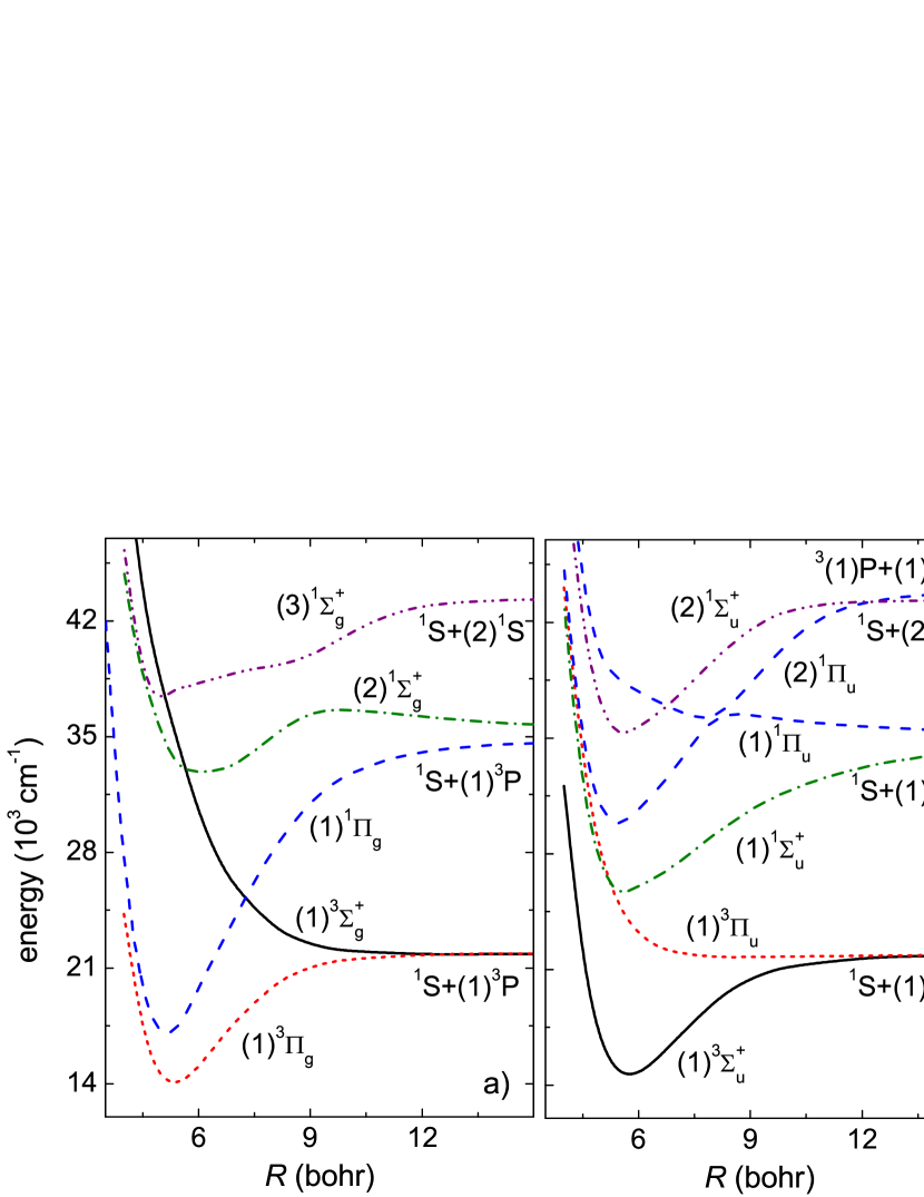
Figure 2: Potential energy curves of the gerade (left panel) and ungerade (right panel) excited states of the magnesium dimer.

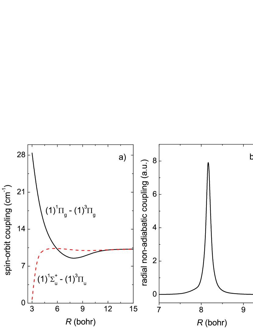
Figure 3: Spin-orbit coupling matrix elements between the $(1)^{1}\Pi_{g}$ and the $(1)^{3}\Pi_{g}$ states, and $(1)^{1}\Sigma_{u}^{+}$ and $(1)^{3}\Pi_{u}$ states (left panel) and radial nonadiabatic coupling between the$(1)^{1}\Pi_{u}$ and $(2)^{1}\Pi_{u}$ states of the Mg₂ molecule.

Potential energy curves for all electronic states computed in the present work are reported in Fig. 2. They all show a smooth behavior with well defined minima and in some cases maxima due to the first-order resonant interactions. The potential energy curves of the A${}^{1}\Sigma_{u}^{+}$ and $(1)^{3}\Pi_{u}$ states and of the $(1)^{1}\Pi_{g}$ and $(1)^{3}\Sigma_{g}^{+}$ cross each other. These crossings should experimentally be observed as a perturbation due to the very weak, but non-zero spin-orbit coupling between the singlet and triplet states. Indeed, the experimental data on the ${\rm A}^{1}\Sigma_{u}^{+}\leftarrow{\rm X}^{1}\Sigma_{g}^{+}$ transitions,Balfour:70 and the UV fluorescence spectra from the $(1)^{1}\Pi_{g}$ state RybakPRL11 ; RybakFaraday confirm weak perturbations due to the spin-orbit coupling. The corresponding matrix elements are shown in Fig. 3. Except for small interatomic distances they show a weak $R$ dependence and smoothly tend to the atomic value. The $(2)^{1}\Sigma_{g}^{+}$ and $(3)^{1}\Sigma_{g}^{+}$ show an avoided crossing, but the gap between the two curves is so large that most probably no homogeneous perturbations will be observed in the spectra. By contrast, the $(1)^{1}\Pi_{u}$ and $(2)^{1}\Pi_{u}$ states show a very pronounced avoided crossing with a gap of a few wavenumbers. This suggests a strong interaction between these states through the radial nonadiabatic coupling matrix element. The shape of this element is shown in the right panel of Fig. 3. As expected, the nonadiabatic coupling matrix element is a smooth Lorenzian-type function, which, in the limit of an inifintely close avoided crossing, becomes a Dirac $\delta$-function. The height and width of the curve depends on the strength of the interaction, and the small width of the coupling in Fig. 3b suggests a strong nonadiabatic coupling. It is gratifying to observe that the maximum on the nonadiabatic coupling matrix element agrees well with the location of the avoided crossing, despite the fact that two very different methods were employed in the ab initio calculations. As discussed above, the potential energy curves were shown to be accurate, so we are confident that also the nonadiabatic coupling matrix element are essentially correct.

The electric transition dipole moments between states $i$ and $f$, $\mu_{j}=\langle\Psi_{i}|\hat{\mu}_{j}|\Psi_{f}\rangle$, where the electric dipole operator, $\hat{\mu}_{j}=r_{j}$, is given by the $j$th component of the position vector and $\Psi_{i/f}$ are the wave functions for the initial and final states, respectively, were computed as the first residue of the LRCCSD linear response function for the $X^{1}\Sigma_{g}^{+}$, ${}^{1}\Pi_{g}$, and ${}^{1}\Pi_{u}(1)$ states. For transitions to the $(2)^{1}\Pi_{u}$ state, the MRCI method was employed. The two-photon transition moment, Eq. (4), can in practice be obtained as a residue of the cubic response function.Olsen:85 For transitions between the $X^{1}\Sigma_{g}^{+}$ and ${}^{1}\Pi_{g}$ states, $M_{ij}^{f\leftarrow 0}(\omega_{L},R)$ was computed as a residue of the coupled cluster cubic response function with electric dipole operators and wave functions within the CCSD framework.Hattig:98a ; Hattig:98b The tensor elements of the electric dipole polarizability of the ground $X^{1}\Sigma_{g}^{+}$ state were obtained as the coupled cluster linear response function with electric dipole operators and wave functions within the CCSD framework.Christiansen:98 The dynamic polarizabilities of the excited states were computed as double residues of the coupled cluster cubic response function with electric dipole operators and wave functions within the CCSD framework.Hattig:98c ; Hattig:98d The nonadiabatic radial coupling matrix elements as well as the spin-orbit coupling matrix elements have been evaluated with the MRCI method.

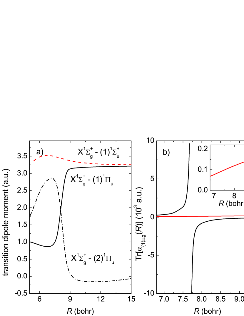
Figure 4: Electric transition dipole moments from the ground electronic state to the three lowest singlet states of ungerade symmetry (left panel), and dynamic Stark shift for the $(1)^{1}\Pi_{g}$ state as obtained from response calculations (black solid line) and after eliminating the contribution from $(2)^{1}\Sigma_{u}^{+}$ state (red dashed line) in the region important for the time-dependent calculations (right panel). The inset illustrates the smooth behavior of the dynamic Stark shift after elimination of the resonance due to the $(2)^{1}\Sigma_{u}^{+}$ state.

The electric transition dipole moments from the ground electronic state to the three lowest singlet states of ungerade symmetry are reported in Fig. 4. The transition moment to the A${}^{1}\Sigma_{u}^{+}$ state is almost constant over a wide range of interatomic distances $R$, and smoothly approaches the atomic value. The transition moments to the $(1)^{1}\Pi_{u}$ and $(2)^{1}\Pi_{u}$ states show more pronounced variations. In fact, the $R$ dependence of these two transition moments reflects the avoided crossing of the corresponding potential energy curves around $R=8.2$ bohr. Also reported in Fig. 4 is the trace of the dynamic Stark shift for the $(1)^{1}\Pi_{g}$ state as a function of $R$. As expected from the definition (6), the dynamic Stark shift shows resonances for transition energies close to the laser frequency $\omega_{L}$. Since the adiabatic elimination that leads to Eq. (6) assumes only non-resonant transitions, the electronic states that cause these resonances need to be included explicitly in the non-perturbative Hamiltonian. This eliminates their contribution to the dynamic Stark shift. Fig. 4b illustrates the procedure, showing the trace of the dynamic polarizability as a function of $R$. The black solid line shows a broad resonance around $R=7.7$ bohr. This resonance corresponds to transitions from the the $(1)^{1}\Pi_{g}$ to the $(2)^{1}\Sigma_{u}^{+}$ state. The latter state is explicitly included in our Hamiltonian for the time-dependent calculations and eliminated from Eq. (6). Once this is done, a smooth and almost constant behavior is obtained, as illustrated in Fig. 4b. Of course, also the contributions from all other electronic states that are explicitly accounted for in the Hamiltonian for the time-dependent calculations are eliminated from Eq. (6).

The Hamiltonian for the time-dependent calculation, neglecting the weak spin-orbit coupling between the $(1)^{1}\Pi_{g}$, $(1)^{3}\Sigma_{g}^{+}$ and $(1)^{3}\Pi_{g}$ states and accounting for states with dipole transitions that are near-resonant to the laser frequency, becomes

$$\boldsymbol{\mathsf{\hat{H}}}_{PA}^{J}(t)=\begin{pmatrix}\boldsymbol{\mathsf{\hat{H}}}^{J}_{X^{1}\Sigma_{g}^{+}}+\omega^{S}_{X^{1}\Sigma_{g}^{+}}(t,R)&\chi^{\star}(t,R)&0&0&0\\ \chi(t,R)&\boldsymbol{\mathsf{\hat{H}}}^{J}_{(1)^{1}\Pi_{g}}+\omega^{S}_{(1)^{1}\Pi_{g}}(t,R)&\mu_{1}(R)E^{\star}(t)&\mu_{2}(R)E^{\star}(t)&\mu_{3}(R)E^{\star}(t)\\ 0&\mu_{1}(R)E(t)&\boldsymbol{\mathsf{\hat{H}}}_{11}^{J}+\omega^{S}_{11}(t,R)&V_{12}(R)+\omega^{S}_{12}(t,R)&0\\ 0&\mu_{2}(R)E(t)&V_{12}(R)+\omega^{S}_{12}(t,R)&\boldsymbol{\mathsf{\hat{H}}}_{22}^{J}+\omega^{S}_{22}(t,R)&0\\ 0&\mu_{3}(R)E(t)&0&0&\boldsymbol{\mathsf{\hat{H}}}^{J}_{(2)^{1}\Sigma_{u}^{+}}\end{pmatrix}\,.$$ (12)

Note that Eq. (12) makes use of the two-photon rotating wave approximation, i.e., the electric field envelope, $E(t)$, in Eq. (3), may be complex, $E(t)=E_{0}S(t)e^{i\varphi(t)}$, and a non-zero $\varphi(t)$ denotes the relative phase with respect to the central laser frequency’s phase. The Hamiltonian (12) is represented on an equidistant grid for each partial wave $J$. Convergence with respect to the grid size $R_{max}$ and number of grid points $N_{R}$ is discussed below in Section IV.

III Quantum dynamical description of a thermal ensemble

The initial state for photoassociation is given by the ensemble of magnesium atoms in the heated cell which interact via the $X^{1}\Sigma_{g}^{+}$ electronic ground state potential. Assuming equilibrium, the initial state is represented by the canonical density operator for $N$ atoms held in a volume $V$ at temperature $T$. Due to the moderate density in a heat pipe, the description can be restricted to atom pairs. The density operator for $N/2$ atom pairs is then obtained from that for a single atom pair, $\boldsymbol{\mathsf{\hat{\rho}}}_{T}(t=0)$, which is expanded into a suitable complete orthonormal basis.MyJPhysB06 Thermally averaged time-dependent expectation values of an observable $\boldsymbol{\mathsf{\hat{A}}}$ are calculated according to

$$\langle\boldsymbol{\mathsf{\hat{A}}}\rangle_{T}(t)=\,\mathsf{Tr}[\boldsymbol{\mathsf{\hat{A}}}\boldsymbol{\mathsf{\hat{\rho}}}_{T}(t)]\,.$$ (13)

The time evolution of $\boldsymbol{\mathsf{\hat{\rho}}}_{T}(t)$ is given by $\boldsymbol{\mathsf{\hat{\rho}}}_{T}(t)=\boldsymbol{\mathsf{\hat{U}}}(t,0)\boldsymbol{\mathsf{\hat{\rho}}}_{T}(t=0)\boldsymbol{\mathsf{\hat{U}}}^{+}(t,0)$ starting from the initial state

$$\boldsymbol{\mathsf{\hat{\rho}}}_{T}(t=0)=\frac{1}{Z}e^{-\boldsymbol{\mathsf{\hat{H}}}/k_{B}T}\,,$$

where $\boldsymbol{\mathsf{\hat{H}}}$ is the Hamiltonian and $Z=\,\mathsf{Tr}[e^{-\boldsymbol{\mathsf{\hat{H}}}/k_{B}T}]$ the partition function. For a thermal, i.e. incoherent, initial state, undergoing coherent time evolution, it is not necessary to solve the Liouville von-Neumann equation for the density operator. Instead, the dynamics can be captured by solving the Schrödinger equation for each basis function. Thermally averaged expectation values are calculated by properly summing over the expectation values obtained from the propagated basis states.MyJPhysB06

Since many scattering states in a broad distribution of rotational quantum numbers are thermally populated, the approach of propagating all thermally populated basis states directlyMyJPhysB06 becomes numerically expensive. Alternatively, an effective description of the thermal ensemble of scattering atoms is obtained by averaging over realizations of random phases. It makes use of thermal random wave functions, $|\psi_{\alpha}^{k}\rangle$. Here, the index $k$ labels a set of random phases and $\alpha$ the basis states. Choosing an arbitrary complete orthonormal basis, $\{|\alpha\rangle\}$, and given that

$$\frac{1}{N}\sum_{k=1}^{N}e^{i(\theta_{\alpha}^{k}-\theta_{\beta}^{k})}=\delta_{\alpha\beta}$$

for random phases $\theta^{k}_{\alpha}$, $\theta^{k}_{\beta}$ and $N$ large, an expansion into random phase wave functions yields a representation of unity,gelmanandronnie

$$\leavevmode\hbox{\small 1\kern-3.3pt\normalsize 1}=\frac{1}{N}\sum_{k=1}^{N}|\Psi^{k}\rangle\langle\Psi^{k}| = \frac{1}{N}\sum_{k=1}^{N}\sum_{\alpha\beta}e^{i(\theta_{\alpha}^{k}-\theta_{\beta}^{k})}|\alpha\rangle\langle\beta|$$ (14)

$$= \frac{1}{N}\sum_{k=1}^{N}\sum_{\alpha\beta}|\Psi^{k}_{\alpha}\rangle\langle\Psi^{k}_{\beta}|\,,$$

where $|\Psi^{k}_{\alpha}\rangle=e^{i\theta_{\alpha}^{k}}|\alpha\rangle$ and $|\Psi^{k}\rangle=\sum_{\alpha}e^{i\theta_{\alpha}^{k}}|\alpha\rangle$.

Here, we use a random phase expansion of unity for the ’vibrational’ degree of freedom, i.e., the radial part $R$ of the relative motion $(R,\theta,\phi)$ of the diatom in its electronic ground state. No electronic excitations are excited thermally. A separation of rotational and vibrational dynamics and subsequent expansion into partial waves is natural to make use of spherical symmetry, $\Psi_{nJM}(R,\theta,\phi)=\varphi_{n}(R|J)\otimes\langle\theta,\phi|J,M\rangle$, i.e., the vibrational motion is conditioned on $J$. This implies a complete set of ’vibrational’ basis functions (both true vibrational eigenfunctions and scattering states), and subsequently, a different set of random phases, for each $J$.

In principle, one could apply a random phase expansion of unity also in the rotational degree of freedom. This would be useful to study the generation of rotational coherence. It requires a model that accounts for rotational coherence, i.e., either a full rovibrational Hamiltonian or, as a minimal approximation, a generalization of Eq. (12) comprising $\boldsymbol{\mathsf{\hat{H}}}^{J+2}_{(1)^{1}\Pi_{g}}$ and $\boldsymbol{\mathsf{\hat{H}}}^{J-2}_{(1)^{1}\Pi_{g}}$ in addition to $\boldsymbol{\mathsf{\hat{H}}}^{J}_{(1)^{1}\Pi_{g}}$. However, in the present work, we focus on the generation of vibrational coherence which is crucial for bond formation.

In the following, we discuss three possible bases for the vibrational Hamiltonian, from which random phase wave functions are generated. All three possibilities will lead, when averaged, to the initial thermal ensemble corresponding to the experiment. While formally equivalent, convergence of the thermal averages with respect to the number of required basis functions differs significantly for the three representations.

III.1 Grid-based random phase approach

The simplest but, as it turns out, most inefficient approach uses, for each partial wave $J$, the coordinate basis of $\delta$-functions localized at each grid point $R$, $\leavevmode\hbox{\small 1\kern-3.3pt\normalsize 1}_{J}=\sum_{R}|R,J\rangle\langle R,J|$.gelmanandronnie A random phase wave function is obtained by multiplying each basis state with a different random phase, $\theta^{k}_{R,J}$,

$$|\Psi^{k}_{J}\rangle=\sum_{R=1}^{N_{R}}e^{i\theta_{R,J}^{k}}|R,J\rangle\,,$$ (15)

with $k$ labeling one realization of $N_{R}$ random phases, $\{\theta^{k}_{R,J}\}$. The resulting wave function, $\langle R|\Psi^{k}_{J}\rangle$, has constant amplitude and a different random phase at each $R$. The initial density operator is obtained by propagating each basis function $|\Psi^{k}_{J}\rangle$ under $\boldsymbol{\mathsf{\hat{H}}}_{g}^{J}=\boldsymbol{\mathsf{\hat{T}}}+V_{g}(R)+\frac{J(J+1)}{2mR^{2}}$ in imaginary time, $\tau=\frac{i}{2}\beta$ with $\beta=1/k_{B}T$, using the Chebychev propagator.RonnieImag86 This yields the thermal random phase wave functions,

$$|\Psi^{k}_{J}\rangle_{T}=e^{-\frac{\beta}{2}\boldsymbol{\mathsf{\hat{H}}}_{g}^{J}}|\Psi^{k}_{J}\rangle$$ (16)

and thus the initial density operator,

$$\boldsymbol{\mathsf{\hat{\rho}}}_{T}(t=0) = \frac{1}{Z}e^{-\frac{\beta}{2}\boldsymbol{\mathsf{\hat{H}}}_{g}}e^{-\frac{\beta}{2}\boldsymbol{\mathsf{\hat{H}}}_{g}}\frac{1}{N}\sum_{k=1}^{N}\sum_{R,R^{\prime},J}(2J+1)e^{i(\theta_{R,J}^{k}-\theta_{n^{\prime},J^{\prime}}^{k})}|R,J\rangle\langle R^{\prime},J|$$ (17)

$$= \frac{1}{Z}\frac{1}{N}\sum_{k=1}^{N}\sum_{J=0}^{J_{max}}(2J+1)e^{-\frac{\beta}{2}\boldsymbol{\mathsf{\hat{H}}}^{J}_{g}}|\Psi^{k}_{J}\rangle\langle\Psi^{k}_{J}|e^{-\frac{\beta}{2}\boldsymbol{\mathsf{\hat{H}}}^{J}_{g}}=\frac{1}{Z}\frac{1}{N}\sum_{k=1}^{N}\sum_{J=0}^{J_{max}}(2J+1)|\Psi^{k}_{J}\rangle_{T}\,{}_{T}\langle\Psi^{k}_{J}|\,.$$

To calculate time-dependent expectation values, $N(J_{max}+1)$ thermal random phase wave functions $|\Psi^{k}_{J}\rangle_{T}$ are propagated in real time,

$$|\Psi^{k}_{J}(t)\rangle_{T}=\boldsymbol{\mathsf{\hat{U}}}(t,0)|\Psi^{k}_{J}\rangle_{T}\,,$$ (18)

with the Hamiltonian (12) as generator. Thermally averaged time-dependent expectation values are obtained from Eq. (13), using cyclic permutation under the trace,

$$\,\mathsf{Tr}\left[\boldsymbol{\mathsf{\hat{A}}}\boldsymbol{\mathsf{\hat{\rho}}}_{T}(t)\right] = \frac{1}{N}\sum_{k=1}^{N}\sum_{R,J}(2J+1)\langle\Psi^{k}_{R,J}|\boldsymbol{\mathsf{\hat{A}}}\boldsymbol{\mathsf{\hat{U}}}(t,0)\boldsymbol{\mathsf{\hat{\rho}}}_{T}(t=0)\boldsymbol{\mathsf{\hat{U}}}^{+}(t,0)|\Psi^{k}_{R,J}\rangle$$ (19)

$$= \frac{1}{Z}\frac{1}{N}\sum_{k=1}^{N}\sum_{R,J}(2J+1)\langle\Psi^{k}_{R,J}|e^{-\frac{\beta}{2}\boldsymbol{\mathsf{\hat{H}}}^{J}_{g}}\boldsymbol{\mathsf{\hat{U}}}^{+}(t,0)\boldsymbol{\mathsf{\hat{A}}}\boldsymbol{\mathsf{\hat{U}}}(t,0)e^{-\frac{\beta}{2}\boldsymbol{\mathsf{\hat{H}}}^{J}_{g}}|\Psi^{k}_{R,J}\rangle$$

$$= \frac{1}{Z}\frac{1}{N}\sum_{k=1}^{N}\sum_{J=0}^{J_{max}}(2J+1)\;_{T}\langle\Psi^{k}_{J}(t)|\boldsymbol{\mathsf{\hat{A}}}|\Psi^{k}_{J}(t)\rangle_{T}\,.$$

Obtaining the $N(J_{max}+1)$ solutions of the Schrödinger equation, $|\Psi^{k}_{J}(t)\rangle_{T}$, required by Eq. (19) requires typically significantly less numerical effort than propagating $(J_{max}+1)$ $N_{R}\times N_{R}$-dimensional density matrices, neglecting the rovibrational coupling, or once the full $N_{R}(J_{max}+1)\times N_{R}(J_{max}+1)$-dimensional density matrix. Note that while $|\Psi^{k}_{J}\rangle_{T}$ has zero components on all electronic states except the ground state, $|\Psi^{k}_{J}(t>0)\rangle_{T}$ will be non-zero for all electronic states due to the interaction with the field. Relevant expectation values are the excited state population after the pump pulse, possibly $J$-resolved. The corresponding operators are the projectors onto the electronically excited state, $\boldsymbol{\mathsf{\hat{P}}}_{e}=|e\rangle\langle e|$, and $\boldsymbol{\mathsf{\hat{P}}}^{J}_{e}$, i.e.,

$$\langle\boldsymbol{\mathsf{\hat{P}}}^{J}_{e}\rangle(t_{f})=\frac{1}{Z}\frac{1}{N}\sum_{k=1}^{N}\sum_{J=0}^{J_{max}}(2J+1)|\langle e|\Psi^{k}_{J}(t_{f})\rangle_{T}|^{2}\,.$$ (20)

The convergence of this approach is slow. The number of realizations required to reach convergence was found to be much larger than the number of grid points. The reason for the slow convergence is that there is no preselection of those basis states that are most relevant in the thermal ensemble. We will therefore not use this method and have included it here only for the sake of completeness.

III.2 Eigenfunction-based random phase approach

A preselection of the relevant states becomes possible by choosing the eigenbasis $|n,J\rangle$ of $\boldsymbol{\mathsf{\hat{H}}}_{g}^{J}$ and evaluating the trace only for basis states with sufficiently large thermal weights, $e^{-E_{n,J}/2k_{B}T}>\epsilon$ where $\epsilon$ is a prespecified error. The eigenfunction-based random phase wave functions are given by

$$|\Psi^{k}_{J}\rangle=\sum_{n}e^{i\theta_{n,J}^{k}}|n,J\rangle\,,$$ (21)

where $J$ denotes the partial wave and $n$ is the vibrational quantum number in the bound part of the spectrum of $\boldsymbol{\mathsf{\hat{H}}}_{g}^{J}$ or, respectively, the label of box-discretized continuum states. It is straightforward to evaluate the representation of the initial density operator in this basis,

$$\boldsymbol{\mathsf{\hat{\rho}}}_{T}(t=0) = \frac{1}{Z}e^{-\frac{\beta}{2}\boldsymbol{\mathsf{\hat{H}}}_{g}}e^{-\frac{\beta}{2}\boldsymbol{\mathsf{\hat{H}}}_{g}}\frac{1}{N}\sum_{k=1}^{N}\sum_{n,n^{\prime},J}(2J+1)e^{i(\theta_{n,J}^{k}-\theta_{n^{\prime},J}^{k})}|n,J\rangle\langle n^{\prime},J|$$ (22)

$$= \frac{1}{Z}\frac{1}{N}\sum_{k=1}^{N}\sum_{n,n^{\prime},J}(2J+1)e^{-\frac{\beta}{2}E_{n,J}+i\theta_{n,J}^{k}}\;e^{-\frac{\beta}{2}E_{n^{\prime},J}-i\theta_{n^{\prime},J}^{k}}\;|n,J\rangle\langle n^{\prime},J|$$

$$= \frac{1}{Z}\frac{1}{N}\sum_{k=1}^{N}\sum_{J=0}^{J_{max}}(2J+1)|\Psi^{k}_{J}\rangle_{T}\,{}_{T}\langle\Psi^{k}_{J}|$$

where $E_{n,J}$ denotes an eigenvalue of the partial wave ground state Hamiltonian, $\boldsymbol{\mathsf{\hat{H}}}_{g}^{J}$, and the $N(J_{max}+1)$ initial random phase wave functions are given by

$$|\Psi^{k}_{J}\rangle_{T}=\sum_{n}e^{-\frac{\beta}{2}E_{n,J}+i\theta_{n,J}^{k}}|n,J\rangle\,.$$ (23)

Thermally averaged time-dependent expectation values are calculated analogously to Eq. (19), where the time-dependent wave functions are obtained by propagating the wave functions of Eq. (23) instead of the initial states given by Eqs. (15) and (16). For convenience, we use normalized random phase wavefunctions instead of Eq. (23),

$$|\tilde{\Psi}^{k}_{J}\rangle_{T}=\frac{1}{\sqrt{Z_{J}^{R_{max}}}}|\Psi^{k}_{J}\rangle_{T}\,,$$ (24)

where $Z_{J}^{R_{max}}=\sum_{n}e^{-\beta E_{n,J}}$ and $R_{max}$ indicates the size of the box. For the thermally averaged time-dependent expectation values, this yields

$$\,\mathsf{Tr}\left[\boldsymbol{\mathsf{\hat{A}}}\boldsymbol{\mathsf{\hat{\rho}}}_{T}(t)\right]=\frac{1}{N}\sum_{k=1}^{N}\sum_{J=0}^{J_{max}}P_{J}\langle\tilde{\Psi}^{k}_{J}(t)|\boldsymbol{\mathsf{\hat{A}}}|\tilde{\Psi}^{k}_{J}(t)\rangle$$ (25)

with

$$P_{J}=\frac{(2J+1)Z_{J}^{R_{max}}}{Z}$$ (26)

the weight of the contribution of partial wave $J$.

The eigenfunction-based random phase approach requires diagonalization of the $J_{max}+1$ partial wave ground state Hamiltonians, $\boldsymbol{\mathsf{\hat{H}}}_{g}^{J}$. Depending on the time required for the propagation of each basis state, this effort may very well be paid off by the much smaller number of basis states that need to be propagated.

The partition function for the computational box of radius $R_{max}$ is straightforwardly evaluated in the eigenbasis,

$$Z_{box}^{R_{max}}=\sum_{J}(2J+1)Z_{J}=\sum_{J=0}^{J_{max}}\sum_{n=0}^{n_{max}}(2J+1)e^{-E_{nJ}/k_{B}T}\,,$$

where $n_{max}$, $J_{max}$ are chosen such that $e^{-E_{n_{max}+1,J_{max}+1}/k_{B}T}<\epsilon$. Since we are interested in high temperatures, it is natural to compare the calculated partition function $Z_{box}$ to its classical approximation,

$$Z_{cl}=\frac{4\pi^{2}}{h^{3}}\sqrt{\frac{2m\pi}{\beta}}\int dJ\,2J\,Z_{J,cl}^{R_{max}}$$ (27)

with

$$Z^{R_{max}}_{J,cl}=R_{max}e^{-\beta\frac{J^{2}}{2mR_{max}^{2}}}-\sqrt{\frac{\pi\beta J^{2}}{2m}}\,\mathsf{erfc}\left(\sqrt{\frac{\beta J^{2}}{2mR_{max}^{2}}}\right)$$ (28)

and $\,\mathsf{erfc}(x)=1-\,\mathsf{erf}(x)$. The derivation of $Z_{cl}$ is given in Appendix A. For a temperature of 1000 K, we find $Z_{box}$ and $Z_{cl}$ to agree within less than 1%. Inserting the classical approximation of $Z^{R_{max}}_{box}$ and $Z_{J}^{R_{max}}$ into Eq. (26), we find $P_{J}$ to roughly correspond to the normalized Boltzmann weight at the end of the grid.

III.3 Freely propagated Gaussian random phase wave packets

The third approach avoids diagonalization of the partial wave ground state Hamiltonians, $\boldsymbol{\mathsf{\hat{H}}}_{g}^{J}$, approximating them by the kinetic energy, $\boldsymbol{\mathsf{\hat{T}}}$, only. This approximation is valid at high temperatures where the kinetic energy of the scattering atoms is much larger than their potential energy due to the inter-particle interaction. It starts from a Gaussian wave paket positioned sufficiently far from the interaction region. If the width of the wave packet is adjusted thermally, projection onto energy resolved scattering wave functions yields Boltzmann weights,

$$|\Psi_{J}^{R_{0}}\rangle_{T}=\frac{1}{(\sqrt{2\pi}\sigma_{R,T})^{1/2}}e^{-\frac{(R-R_{0})^{2}}{2\sigma_{R,T}^{2}}}|R,J\rangle\,.$$ (29)

The thermal width is given by $\sigma_{R,T}=1/\sigma_{P,T}=1/\sqrt{2m/\beta}=1/\sqrt{2mk_{B}T}$, and $R_{0}\gg R_{V}$ where $R_{V}$ is the interaction region. The Fourier transformed wave packet,

$$|\tilde{\Psi}_{J}^{R_{0}}\rangle_{T}=\frac{1}{(\sqrt{2\pi}\sigma_{P})^{1/2}}e^{-\frac{P^{2}}{2\sigma_{P,T}^{2}}+iPR_{0}}|P,J\rangle\,,$$

corresponds to eigenstates of the kinetic energy with Boltzmann weights,JiriPRA01 i.e., we approximate $e^{-\frac{\beta}{2}\boldsymbol{\mathsf{\hat{H}}}_{g}^{J}}|P,J\rangle\approx e^{-\frac{\beta}{2}\frac{\boldsymbol{\mathsf{\hat{P}}}^{2}}{2m}}|P,J\rangle$. Random phase wave functions can be generated from Eq. (29) by real-time propagation under $\boldsymbol{\mathsf{\hat{H}}}_{g}^{J}$ as follows. The time-evolved wave packet at time $\tau^{k}$ is written as

$$|\Psi_{J}^{R_{0}}(\tau^{k})\rangle_{T}=\sum_{n>n_{0}}c_{nJ}e^{-\frac{\beta}{2}E_{n,J}-iE_{n,J}\tau^{k}+i\theta^{0}_{n,J}}|n,J\rangle\,,$$ (30)

where expansion into the scattering states of the finite computation box, i.e., the states $|n,J\rangle$ with positive energy ($n>n_{0}$), has been used. $\theta^{0}_{n,J}$ is an initial phase due to $R_{0}$. Comparing to Eq. (23), the random phases are given by $\theta^{k}_{n,J}=-E_{n,J}\tau^{k}$. For sufficiently large times, $\tau^{k}\gg\beta/2$ and $v\tau^{k}\gg R_{0}$ which, with $v=p/m=\sqrt{2E/m}=\sqrt{\beta/m}$ yields $\tau^{k}\gg R_{0}\sqrt{m/\beta}$, the wave function will spread significantly and fill the interaction region which is a prerequisite to correctly represent the thermal density. A different set of phases is obtained by propagating the Gaussian wave packet under $\boldsymbol{\mathsf{\hat{H}}}_{g}^{J}$ for a time $\tau^{k^{\prime}}$. For Mg₂ and $T=1000\,$K, the two limits translate into $\tau^{k}\gg 4\,$fs and $\tau^{k}\gg 300\,$ps for $R_{0}=35\,$a₀. For large grids, these numbers grow correspondingly. Moreover, to reproduce the Boltzmann ensemble not only qualitatively, but also quantitatively, the smallest frequency difference between scatterings states in the computation box needs to be resolved. This translates into even longer propagation times.

Practically, a coordinate grid based wave packet, Eq. (29), is propagated under $\boldsymbol{\mathsf{\hat{H}}}_{g}^{J}$ by a Chebychev propagator where each realization corresponds to a different time $\tau^{k}$. The density operator is constructed by averaging over the times, $\tau^{k}$, chosen randomly. Alternatively, if the eigenvalues $E_{n,J}$ and eigenstates $|n,J\rangle$ are known, the thermal random phase wavefunctions can be obtained simply by projection on the $|n,J\rangle$, choice of a random phase and reassembly of the Gaussian wavepacket from the random-phase projections. This avoids the very long propagation times required to faithfully represent the Boltzmann ensemble. The method of choice, diagonalization of the ground state Hamiltonians, $\boldsymbol{\mathsf{\hat{H}}}_{g}^{J}$, and subsequent projection, or propagation under $\boldsymbol{\mathsf{\hat{H}}}_{g}^{J}$ depends on the dimensionality of the problem due to the different scaling of diagonalization and propagation. For a diatomic, the diagonalization approach was found to be more efficient. For larger systems, the propagation approach is expected to take over.

The convergence of random phase wave functions built on thermal Gaussians with respect to the photoassocation yield is comparatively fast, only a few realizations are sufficient. The drawback of the procedure is that only the free part of the initial wave functions is represented, leaving out the interaction energy of the true scattering states as well as initial population in bound or quasi-bound states. Thermal expectation values are obtained according to Eq. (25) where $|\tilde{\Psi}_{J}^{k}\rangle_{T}=e^{-i\boldsymbol{\mathsf{\hat{H}}}_{g}^{J}\tau^{k}}|\Psi^{R_{0}}_{J}\rangle_{T}$ is a (normalized) Gaussian random packet, freely propagated for random times $\tau^{k}$. The probability $P_{J}$ for partial wave $J$, Eq. (26), needs to account for the fact that the Gaussian is initially positioned at $R_{0}$, not the edge of the grid. Therefore, using the classical approximation, $R_{max}$ in Eq. (26) needs to be replaced by $R_{0}$.

Another variant utilizes $\delta$-functions in momentum space, $\leavevmode\hbox{\small 1\kern-3.3pt\normalsize 1}_{J}=\frac{1}{N}\sum_{k=1}^{N}\sum_{P,P^{\prime}}|P,J\rangle\langle P^{\prime},J|$, and add random phases, $\theta^{k}_{P,J}$, to the momentum components directly,

$$|\Psi^{k}_{P,J}\rangle=e^{i\theta^{k}_{P,J}}|P,J\rangle\,.$$

The random phases, $\theta^{k}_{P,J}$, translate into positions of the Gaussian, $R^{k}_{0}$. This procedure reconstructs the correct density in the regions of flat potential but fails in the interaction region and is therefore not employed here.

III.4 Calculating the quantum mechanical purity of a thermal ensemble

The laser pulse excites a small fraction of the incoherent ensemble of ground state atom pairs to the $(1)^{1}\Pi_{g}$ state and further to the first and second ${}^{1}\Pi_{u}$ state. This action corresponds to distillation and leads to higher purity and coherence of the photoassociated molecules.RybakPRL11 In order to study the purity of the subensemble of diatoms in the excited electronic state,

$$\mathcal{P}_{e}(t)=\,\mathsf{Tr}[\boldsymbol{\mathsf{\hat{\rho}}}^{2}_{T,e}(t)]\,,$$ (31)

the normalized density operator of electronic state $|e\rangle$, is formally constructed,

$$\boldsymbol{\mathsf{\hat{\rho}}}_{T,e}(t) = \frac{1}{\langle\boldsymbol{\mathsf{\hat{P}}}_{e}\rangle(t)}\frac{1}{N}\sum_{k=1}^{N}\sum_{J=0}^{J_{max}}P_{J}\,\boldsymbol{\mathsf{\hat{P}}}_{e}|\tilde{\Psi}^{k}_{J}(t)\rangle_{T}\,{}_{T}\langle\tilde{\Psi}^{k}_{J}(t)|\boldsymbol{\mathsf{\hat{P}}}_{e}\,.$$ (32)

In the grid representation using $N_{R}$ grid points, $\boldsymbol{\mathsf{\hat{\rho}}}_{T,e}(t)$ becomes a matrix of size $N_{R}\times N_{R}$,

$$\rho_{T,e}(R,R^{\prime};t) = \frac{1}{\langle\boldsymbol{\mathsf{\hat{P}}}_{e}\rangle(t)}\frac{1}{N}\sum_{k=1}^{N}\sum_{J=0}^{J_{max}}P_{J}\,\tilde{\Psi}^{k,e}_{T,J}(R,t)\;\tilde{\Psi}^{{k,e}^{\star}}_{T,J}(R^{\prime},t)\,,$$

where $\tilde{\Psi}^{k,e}_{T,J}(R,t)=\langle R,e|\tilde{\Psi}^{k}_{J}(t)\rangle_{T}$ is the excited state projection of the ($k,J$)th propagated thermal random phase wave function, $\langle R|\tilde{\Psi}^{k}_{J}\rangle_{T}$. Since we expect to populate only a limited number of $(1)^{1}\Pi_{g}$ state eigenfunctions, say $N_{m}$, it is computationally advantageous to transform the excited state component of the propagated thermal wave functions into the rovibrational eigenbasis, $|\varphi^{e}_{mJ}\rangle$, of the $(1)^{1}\Pi_{g}$ state,

$$\tilde{\Psi}^{k,e}_{T,J}(R,t)=\sum_{m=0}^{N_{m}-1}c^{k,T}_{mJ}(t)\varphi^{e}_{mJ}(R)\,,$$

with

$$c^{k,T}_{mJ}(t)=\int\tilde{\Psi}^{k,e}_{T,J}(R,t)\varphi^{e*}_{mJ}(R)\,dR\,.$$

The resulting density matrix,

$$\rho_{T,e}^{m,m^{\prime}}(t) = \frac{1}{\langle\boldsymbol{\mathsf{\hat{P}}}_{e}\rangle(t)}\frac{1}{N}\sum_{k=1}^{N}\sum_{J=0}^{J_{max}}P_{J}\,c^{k,T}_{mJ}(t)c^{{k,T}^{\star}}_{m^{\prime}J}(t)\,,\quad m,m^{\prime}=0,\ldots,N_{m}-1\,,$$

is only of size $N_{m}\times N_{m}$ and can more efficiently be squared to obtain the purity. Moreover, this representation lends itself naturally to the evaluation of the dynamical coherence measure. In the eigenbasis, we can decompose the density operator into its static (diagonal) and dynamic (off-diagonal) part, $\boldsymbol{\mathsf{\hat{\rho}}}=\boldsymbol{\mathsf{\hat{\rho}}}_{stat}+\boldsymbol{\mathsf{\hat{\rho}}}_{dyn}$. Such a decomposition has been motivated in the study of dissipative processes, in particular by the fact that pure dephasing does not alter the static part.BaninJCP94 ; BaninCP94 The dynamical coherence measure,

$$\mathcal{C}_{e}(t)=\,\mathsf{Tr}[\boldsymbol{\mathsf{\hat{\rho}}}^{2}_{T,e,dyn}(t)]\,,$$ (33)

captures the part of the purity that arises from the dynamical part of the density operator.BaninJCP94 ; BaninCP94

The purity of the excited state subensemble after the pump pulse, $\mathcal{P}_{e}(t_{f})$, shall be compared to the initial purity of the whole ensemble (in the electronic ground state),

$$\mathcal{P}_{g}(t=0)=\,\mathsf{Tr}[\boldsymbol{\mathsf{\hat{\rho}}}^{2}_{T}(t=0)]\,.$$

To this end, but also to determine the photoassociation probability, cf. Eq. (20), the partition function $Z$ needs to be determined explicitly. We need to take into account that our computation box represents only a small part of the experimental volume. The total partition function is therefore given by $Z=Z_{box}\frac{V}{V_{box}}$, where $V_{box}=\frac{4}{3}\pi R_{max}^{3}=4.97\times 10^{-18}\,$cm³ for $R_{max}=200\,$a₀ and $V$ the experimental volume. Alternatively, the probability of a single atom in our computation box is $p_{box}=\rho V_{box}$ with $\rho$ the experimental density, $\rho=4.8\times 10^{16}$ atoms/cm³. The probability of finding two atoms in the box is then simply $p^{2}_{box}=5.7\times 10^{-2}$. Using Eq. (25) with $\boldsymbol{\mathsf{\hat{A}}}=\leavevmode\hbox{\small 1\kern-3.3pt\normalsize 1}$, the purity of the initial state is obtained as

$$\mathcal{P}_{g}(t=0)=p_{box}^{2}\sum_{J=0}^{J_{max}}P_{J}^{2}\,,$$ (34)

taking $Z=Z_{box}$ in Eq. (26) when evaluating $P_{J}$.

IV Convergence of the thermal averaging procedures: Photoassociation probability

The interaction of the atom pair with the laser field is simulated by solving $N(J_{max}+1)$ time-dependent Schrödinger equations,

$$i\hbar\frac{\partial|\psi_{J}^{k}(t)\rangle_{T}}{\partial t}=\boldsymbol{\mathsf{\hat{H}}}^{J}_{PA}(t)|\psi_{J}^{k}(t)\rangle_{T}\,,$$ (35)

for $k=1,\ldots,N$ and $J=0,\ldots,J_{max}$, with a Chebychev propagatorchebyprop and thermally averaging the solutions according to Eq. (19). To reduce the computational effort, we evaluate all sums over $J$ in steps of five.

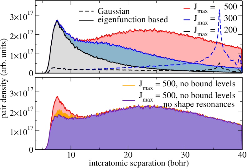
Figure 5: Initial thermal density $\rho_{T,g}(R)/R^{2}$ of ground state atom pairs (calculated using Eq. (22) with 200 realizations for each $J$ and excluding bound states and shape resonances from the sum over $k$).

We first study the initial thermal density of atom pairs, cf. Eq. (22), that is excited by the laser pulse. It sets a limit to the excitation yield since thermalization occurs over timescales larger than that of the experiment. The initial thermal density of atom pairs is shown as a function of interatomic distance in Fig. 5 for random phase wave functions built from eigenfunctions, cf. Eq. (24) and built from Gaussians, cf. Eq. (30). For photoassociation, distances smaller than $\sim 12\,a_{0}$ are relevant. The thermal density is converged in this region by including rotational quantum numbers up to $J=300$. The contribution of higher partial waves only ensures a constant density at large interatomic distances. The long-distance part naturally converges very slowly but this is irrelevant for the dynamical calculations. The peak at short interatomic separations is due to bound levels, shape resonances and the classical turning point of the scattering states at the repulsive barrier of the potential: The difference between the red and orange curves in Fig. 5 indicates the contribution of bound levels, the difference between the orange and the purple curve that of shape resonances.

The Gaussian method requires much larger grids than the eigenfunction based method to converge the initial thermal density since it is based on the assumption that the effective potential is zero at the position of the Gaussians. However, for large values of $J$, the rotational barrier is non-zero even at comparatively large internuclear separations. This leads to a spurious trapping of probability amplitude, cf. the dashed curves in Fig. 5. At short internuclear separations, the pair density calculated from thermal Gaussians in the upper panel of Fig. 5 shows the same behavior as the purple curve in the lower panel of Fig. 5 (up to scaling which is due to the accumulation of amplitude at large internuclear separations). This indicates that random phase wave functions built from thermal Gaussians do not capture bound states and shape resonances.

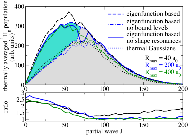
Figure 6: Top panel: Thermally-averaged population of the ${}^{1}\Pi_{g}$ state, calculated as $Z\langle\boldsymbol{\mathsf{\hat{P}}}_{e}\rangle$, vs initial partial wave $J$, averaged over 200 realizations of random phase wave functions, for three different grid sizes $R_{max}$ and a transform-limited pulse with $I_{0}=5\times 10^{12}\,$W/cm² and $\tau=100\,$fs (excluding the bound states and shape resonances from the sum over $k$ in Eq. (25)). The light-blue shaded part indicates the contribution of scattering states, i.e., photoassociation, for $R_{max}=200\,$a₀. The contributions of the shape resonances is given by the difference between the blue solid and dashed curves. Propagating random phase wave functions calculated from thermal Gaussians, cf. Eq. (30), does not capture excitation of bound levels and shape resonances (dotted curves). Bottom panel: Ratio of the excitation yields calculated from random phase wavefunctions based on eigenfunctions and thermal Gaussians. For large $J$ and sufficiently large grid size, the two methods coincide as expected.

These two features of the Gaussian random phase wave functions show also up in the population transferred from the initial incoherent ensemble to the ${}^{1}\Pi_{g}$ state, shown in Fig. 6. The thermal averaging procedure has been repeated for increasing initial rotational quantum number, $J$. That is, for each rotational barrier, eigenfunction-based and Gaussian random phase wave functions are propagated in real time with the full, time-dependent Hamiltonian, $\boldsymbol{\mathsf{\hat{H}}}_{PA}^{J}$. Expectation values, such as the population of the ${}^{1}\Pi_{g}$ state after the pump pulse is over, are calculated for each random phase realization, $k$, and averaged over, including the rotational degeneracy factor $J+1$, cf. Eq. (19). For large grids ($R_{max}=200\,$a₀, $R_{max}=400\,$a₀) and large $J$, random phase wave functions built from eigenfunctions and built from thermal Gaussians yield the same results. Due to the trapping of probability amplitude at large internuclear separations, for small grids ($R_{max}=40\,$a₀) and large $J$, the Gaussian method underestimates the excitation yield. Since our random phase wave functions are normalized in the computation box, this results in an initial thermal density which is too small at the internuclear separations, $R\sim 7\,$a${}_{0}\ldots 9\,$a₀, that are relevant for the laser excitation. This is illustrated by the black curve in the lower panel of Fig. 6 which deviates from the blue and green curves even for large $J$. For $J\leq 75$, the potential supports bound levels which are not captured by the Gaussian random phase wave functions. Once the bound levels and shape resonances are removed from the eigenfunction based approach (solid blue curve), the eigenfunction-based approach roughly agrees with the Gaussian approach (blue dotten curve). This comparison allows for estimating the contribution of the bound levels. For $J\geq 75$ the ground state potential does not support any bound levels due to the high centrifugal barrier. The total contribution of the bound part of the spectrum to the excitation of ${}^{1}\Pi_{g}$ population amounts to about 20%. The differences between $J=75$ to $J=95$ are attributed to insufficient sampling of the free propagation method.

Qualitatively, however, the two approaches yield the same result with a steep rise at low $J$-values, a peak at intermediate $J$ and an exponential tail for $J\geq 100$. The peak is shifted toward larger $J$ for the Gaussian method since it cannot capture the excitation of bound levels and shape resonances. Each random phase approach represents a statistical sampling of the photoassociation yield. The deviation of an expectation value from its mean scales as $1/\sqrt{N}$ where $N$ is the number of realizations. This was checked for $J=55$ and $J=100$ the pre-factor $\sigma/mean=\bar{s}/\sqrt{N}$ is estimated as $\bar{s}\sim 0.37$ for the free propagation method and $\bar{s}\sim 0.17$ for the eigenvalue method (note that $s\sim 0.30$ for the grid based method). This makes the eigenvalue method converge fastest.

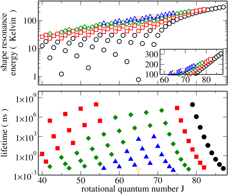
Figure 7: Top panel: Position of shape resonances vs initial partial wave $J$. Bottom panel: Lifetimes in nanoseconds of the high-lying shape resonances vs partial wave $J$.

The shape resonances are analyzed in Fig. 7 which displays their position in energy (top panel) and the lifetimes of those shape resonances that are sufficiently short lived, i.e., sufficiently broad, to contribute to the photoassociation process (bottom panel). The shape resonances were calculated using a complex absorbing potential.NimrodPhysRep98 Shape resonances are found for $J=40,\ldots,87$. The positions of the short-lived resonances lie between 15 K and 300 K. With a sample temperature of 1000 K i.e., at least the higher lying of these resonances are thermally populated. It is therefore not surprising that a contribution of the shape resonances is observed for $J=45\ldots,85$, cf. the difference between the solid and dashed curves in Fig. 6. The contribution is easily rationalized by the shape resonances representing quasi-bound states that are ideally suited for photoassociation.GonzalezKochPRA12 They give structure to the continuum of scattering states which otherwise is completely flat at high temperature. This can be utilized for generation of coherence and control.

In conclusion, the random phase wave functions built from thermal Gaussians can be used if a rough estimate of the photoassociation yield is desired. When further refinement is required the eigenvalue approach converges faster by a factor of 2. Since the Gaussian approach excludes the bound part of the spectrum and the resonances, it comes with error bars of about 20%. If more accurate results are desired, the eigenfunction based random phase approach is the method of choice. The eigenfunction based method is also best suited to capture the contribution of bound states and shape resonances to the photoassociation yield.

V Interplay of coherence and photoassociation yield

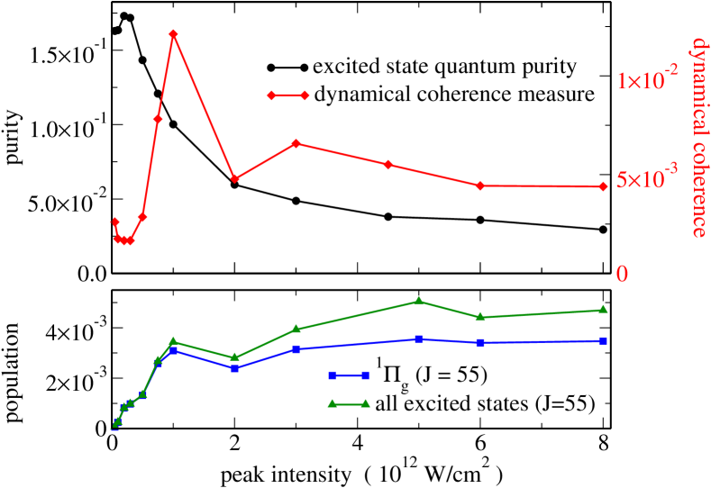
Figure 8: Top panel: Excited state purity, $\mathcal{P}^{box}_{e}(t_{final})$, and coherence measure, $\mathcal{C}_{e}(t_{final})$, cf. Eqs. (31) and (33), vs pulse intensity for the subensemble of photoassociated molecules. Bottom panel: Photoassociation yield for $J=55$ as a function of peak pulse intensity. All calculations employ transform-limited pulses of 100 fs full-width at half maximum.

The degree of distillation of coherence out of an incoherent initial ensemble can be rationalized and quantified by considering the enhancement of quantum purity ${\cal P}=\,\mathsf{Tr}[\boldsymbol{\mathsf{\hat{\rho}}}^{2}]$ and coherence. The experimental signature is the periodic modulation of the pump probe signal.RybakPRL11 ; RybakFaraday The purity for an incoherent ensemble is inversely proportional to the number of occupied quantum states of a pair of atoms. This number is completely determined by the temperature $T=1000\,$K, and density, $\rho=4.8\cdot 10^{16}\,$atoms/cm³, in the experiment. The bandwidth of our pulse plus Stark shift largely exceeds the thermal width. This implies that all atom pairs within the Franck-Condon window are excited on equal ground, irrespective of their collision energy. We partition the total volume into identical smaller volumes containing exactly one pair of atoms such that the smaller volume corresponds to our computation box.MyJPhysB06 The initial purity of the atom pair in our computation box of volume $V_{box}$ is given by the ground state purity, ${\cal P}_{g}^{box}$, multiplied by the probability for two atoms to occupy this box, ${\cal P}^{g}=p^{2}{\cal P}_{g}^{box}$, cf. Section III.4. The initial ground state purity is bounded from below by the purity of a maximally mixed state represented in our box. For $N=200$ random phase realizations and $J_{max}=200/5$ we estimate the lower bound to be $1\times 10^{-4}$. Evaluating ${\cal P}_{g}^{box}$ using the classical approximation for $P_{J}$ in Eq. (34) we obtain ${\cal P}_{g}^{box}=3.3\times 10^{-4}$ for $R_{max}=200\,$a₀ and $T=1000\,$K and thus ${\cal P}_{g}=1.9\times 10^{-5}$ for the initial purity.

For the ensemble of molecules in the electronically excited ${}^{1}\Pi_{g}$ state, the density operator is given by Eq. (32) and the purity within the computational box by Eq. (31). The actual excited state purity is obtained by multiplying Eq. (31) by the probability for finding two atoms to be in the computational box, $p^{2}$. Note that the excited state density operator is normalized with respect to the excitation yield, $\langle\boldsymbol{\mathsf{\hat{P}}}_{e}\rangle$. We obtain a purity ${\cal P}_{e}^{box}\approx 5\cdot 10^{-2}$ for the molecular sub-ensemble in the ${}^{1}\Pi_{g}$ excited state for the experimental pulse parameters. We thus observe a significant increase in the quantum purity, $\,\mathsf{Tr}[\boldsymbol{\mathsf{\hat{\rho}}}^{2}]$, induced by the femtosecond laser pulse. The underlying physical mechanism can be viewed as ”Franck-Condon filtering”: for a given initial $J$ value there is only a limited range of collision energies that allow the colliding pair to reach the Franck-Condon window for PA located at short internuclear distancesBackhausCP97 .

In order to obtain a quantitative estimate of the degree of distillation achieved by the femtosecond photoassociation process, we have calculated the purity of the ensemble of photoassociated molecules in the ${}^{1}\Pi_{g}$ state for a range of laser intensities, cf. Fig. 8. For weak fields, the purity is roughly constant as a function of intensity and about three times larger than the purity obtained for the intensity of $5\times 10^{12}\,$W/cm² used in the experiment. As intensity is increased, a drop in the purity is observed which levels off at large intensities. We attribute this drop to power broadening for strong fields, which brings more atom pairs into the Franck-Condon window for PA.

The purity of the photoassociated sub-ensemble is less than the inverse of the number of occupied energy states due to coherence. To quantify this effect we separate static and dynamic contributions, $\boldsymbol{\mathsf{\hat{\rho}}}=\boldsymbol{\mathsf{\hat{\rho}}}_{stat}+\boldsymbol{\mathsf{\hat{\rho}}}_{dyn}$. Expressing the density operator $\boldsymbol{\mathsf{\hat{\rho}}}$ in the energy representation the static part corresponds to the diagonal matrix elements and the dynamical coherence to the off-diagonal elements. The dynamical contributions are quantified by the coherence measure ${\cal C}=\,\mathsf{Tr}[\boldsymbol{\mathsf{\hat{\rho}}}^{2}_{dyn}(t)]$.BaninJCP94 . Figure 8 shows the coherence measure of the excited state, ${\cal C}^{e}$, as a function of laser intensity (red diamonds). It is found to be about one order of magnitude smaller than the purity. This is rationalized by the change in Franck-Condon points with different $J$ which degrade the vibrational coherence. Within a sub-ensemble for a given angular momentum $J$ the difference between ${\cal C}_{J}^{e}$ and ${\cal P}_{J}^{e}$ is less than an order of magnitude.

VI Conclusions

We have described two-photon femtosecond photoassociation of magnesium atoms from first principles using state of the art ab initio methods and quantum dynamical calculations. Highly accurate potential energy curves were obtained using the coupled cluster method and a large basis set. Two-photon couplings and dynamic Stark shifts are important to correctly model the interaction of the atom pairs with the strong field of a femtosecond laser pulse. They were calculated within the framework of the equation of motion (response) coupled cluster method. The photoassociation dynamics were obtained by solving the time-dependent Schrödinger equation for all relevant partial waves, accounting for the laser-matter interaction in a non-perturbative way, and performing a thermal average.

We have developed an efficient numerical method to describe the incoherent thermal ensemble that is the initial state for photoassociation at high temperatures. It is based on random phase wave packets which can be built from eigenfunctions of the grid, the Hamiltonian, or the kinetic energy. The latter can provide a rough estimate which is sufficient to yield qualitatively correct results. It neglects, however, the contribution from bound levels and long-lived shape resonances and therefore comes with error bars of about 20%. The best compromise between high accuracy and convergence is found for the eigenfunction-based method where random phase realizations are built from the eigenfunctions of the electronic ground state Hamiltonian. About 200 partial waves and 200 realizations for each partial wave are required for converged photoassociation dynamics. Time-dependent thermal averages are obtained by propagating each of the random phase wave functions and incoherently summing up all single expectation values.

The random phase approach allows for constructing the thermal atom pair density as a function of interatomic separation for high temperatures. This is important to highlight the difference between hot and cold photoassociation.VardiJCP97 ; JiriPRA01 ; MyJPhysB06 In the cold regime, the largest density is defined by the quantum reflection and resides in the long-distance, downhill part of the potential. The opposite is true in the hot regime: Here, the largest density is found in the repulsive part of the ground state potential. This is due to the many partial waves that are thermally populated and the colliding atom pairs having sufficiently high kinetic energy to overcome the rotational barriers. For specific partial waves, shape resonances are found to play a role. This is not surprising since they represent quasi-bound states that are ideally suited for photoassociation.GonzalezKochPRA12 At very low temperatures, most partial waves are frozen out and the scattering is almost exclusively $s$-wave. The role of the rotational quantum numbers $J$ is less important in the electronically excited state but it is still detectable in form of quantum beats.RybakPRL11 Both hot and cold photoassociation come with advantages as well as drawbacks. In the hot regime, molecules with much shorter bond length than in the cold regime are formed. However, the quantum purity and coherence of the created molecules is much larger in the cold regime where dynamical correlations exist prior to photoassociation. These correlations indicate pre-entanglement of the atom pair. Making a molecule corresponds to entangling two atoms, and photoassociation amounts to filtering out an entangled subensemble both in the hot and cold regime.

Our work has opened up the possibility to study femtosecond photoassociation and its control at high temperatures and to investigate systematically the generation of coherence out of an incoherent initial state. Future efforts will address the efficient theoretical description of the probe step. The theme of coherent control of binary reactions requires a sound theoretical basis to which our current study lays the ground work.

Appendix A Classical approximation of the partition function

The classical approximation of the partition function is obtained starting from the standard definition,

$$Z_{cl}=\frac{1}{h^{3}}\int d^{3}R\int d^{3}Pe^{-\beta\left(\frac{\vec{P}^{2}}{2m}+V(R)\right)}\,.$$

Performing the integral over angles and introducing polar momentum coordinates, we find

$$Z_{cl} = \frac{4\pi}{h^{3}}\int_{0}^{R_{max}}dRR^{2}e^{-\beta V(R)}$$

$$\quad\quad 2\pi\int_{-\infty}^{\infty}dP_{R}\int_{-\infty}^{\infty}dP_{\perp}P_{\perp}e^{-\frac{\beta}{2m}(P_{R}^{2}+P_{\perp}^{2})}$$

$$= \frac{4\pi^{2}}{h^{3}}\int_{0}^{\infty}2JdJ\int_{0}^{R_{max}}dRe^{-\beta\left(V(R)+\frac{J^{2}}{2mR^{2}}\right)}$$

$$\quad\quad\int_{-\infty}^{\infty}dP_{R}e^{-\beta\frac{P_{R}^{2}}{2m}}\,,$$

where we made use of $J=RP_{\perp}$. Carrying out the integral over the radial momentum yields

$$Z_{cl}=\frac{4\pi^{2}}{h^{3}}\sqrt{\frac{2m\pi}{\beta}}\int 2JdJ\int dRe^{-\beta\left(V(R)+\frac{J^{2}}{2mR^{2}}\right)}\,.$$

Approximating the potential $V(R)\approx 0$, the integral over the computational box of size $R_{max}$ can be performed,

$$Z_{cl} = \frac{4\pi^{2}}{h^{3}}\sqrt{\frac{2m\pi}{\beta}}\int dJ\,2J\,Z_{J}^{R_{max}}$$

with

$$Z_{J}^{R_{max}} = \sqrt{\frac{\pi\beta J^{2}}{2m}}\left[\mathrm{erf}\left(\frac{1}{R_{max}}\sqrt{\frac{\pi\beta J^{2}}{2m}}\right)-1\right]$$

$$+R_{max}e^{-\beta\frac{J^{2}}{2mR_{max}^{2}}}\,.$$

References

- (1) R. Kosloff, S. Rice, P. Gaspard, S. Tersigni, and D. Tannor, Chem. Phys. 139, 201 (1989).
- (2) S. A. Rice and M. Zhao, Optical control of molecular dynamics, John Wiley & Sons, 2000.
- (3) P. Brumer and M. Shapiro, Principles and Applications of the Quantum Control of Molecular Processes, Wiley Interscience, 2003.
- (4) D. J. Tannor, Introduction to Quantum Mechanics: A time-dependent perspective, Palgrave Macmillan, 2007.
- (5) R. J. Gordon and S. A. Rice, Annu. Rev. Phys. Chem. 48, 601 (1997).
- (6) T. Brixner and G. Gerber, ChemPhysChem 4, 418 (2003).
- (7) M. Dantus and V. V. Lozovoy, Chem. Rev. 104, 1813 (2004).
- (8) M. Wollenhaupt, V. Engel, and T. Baumert, Annu. Rev. Phys. Chem. 56, 25 (2005).
- (9) O. Kühn and L. Wöste, editors, Analysis and control of ultrafast photoinduced reactions, Springer, Berlin, 2007.
- (10) U. Marvet and M. Dantus, Chem. Phys. Lett. 245, 393 (1995).
- (11) P. Backhaus and B. Schmidt, Chem. Phys. 217, 131 (1997).
- (12) P. Gross and M. Dantus, J. Chem. Phys. 106, 8013 (1997).
- (13) P. Backhaus, J. Manz, and B. Schmidt, J. Phys. Chem. A 102, 4118 (1998).
- (14) P. Backhaus, B. Schmidt, and M. Dantus, Chem. Phys. Lett. 306, 18 (1999).
- (15) R. de Vivie-Riedle, K. Sundermann, and M. Motzkus, Faraday Discuss. 113, 303 (1999).
- (16) M. Bonn, S. Funk, C. Hess, D. N. Denzler, C. Stampfl, M. Scheffler, M. Wolf, and G. Ertl, Science 285, 1042 (1999).
- (17) D. Geppert, A. Hofmann, and R. de Vivie-Riedle, J. Chem. Phys. 119, 5901 (2003).
- (18) P. Nuernberger, D. Wolpert, H. Weiss, and G. Gerber, Proc. Natl. Acad. Sci. USA 107, 10366 (2010).
- (19) V. Zeman, M. Shapiro, and P. Brumer, Phys. Rev. Lett. 92, 133204 (2004).
- (20) K. M. Jones, E. Tiessinga, P. D. Lett, and P. S. Julienne, Rev. Mod. Phys. 78, 483 (2006).
- (21) C. P. Koch and R. Kosloff, Phys. Rev. Lett. 103, 260401 (2009).
- (22) P. Pellegrini, M. Gacesa, and R. Côté, Phys. Rev. Lett. 101, 053201 (2008).
- (23) S. V. Alyabyshev and R. V. Krems, Phys. Rev. A 82, 030702 (2010).
- (24) R. González-Férez and C. P. Koch, Phys. Rev. A 86, 063420 (2012).
- (25) W. Salzmann, T. Mullins, J. Eng, M. Albert, R. Wester, M. Weidemüller, A. Merli, S. M. Weber, F. Sauer, M. Plewicki, F. Weise, L. Wöste, and A. Lindinger, Phys. Rev. Lett. 100, 233003 (2008).
- (26) A. Merli, F. Eimer, F. Weise, A. Lindinger, W. Salzmann, T. Mullins, S. Götz, R. Wester, M. Weidemüller, R. Ağanoğlu, and C. P. Koch, Phys. Rev. A 80, 063417 (2009).
- (27) C. P. Koch, E. Luc-Koenig, and F. Masnou-Seeuws, Phys. Rev. A 73, 033408 (2006).
- (28) C. P. Koch, M. Ndong, and R. Kosloff, Faraday Disc. 142, 389 (2009).
- (29) M. Tomza, M. H. Goerz, M. Musiał, R. Moszynski, and C. P. Koch, Phys. Rev. A 86, 043424 (2012).
- (30) L. Rybak, S. Amaran, L. Levin, M. Tomza, R. Moszynski, R. Kosloff, C. P. Koch, and Z. Amitay, Phys. Rev. Lett. 107, 273001 (2011).
- (31) L. Rybak, Z. Amitay, S. Amaran, R. Kosloff, M. Tomza, R. Moszynski, and C. P. Koch, Faraday Discuss. 153, 383 (2011).
- (32) Y. Silberberg, Annu. Rev. Phys. Chem. 60 (2009).
- (33) K. D. Bonin and V. V. Kresin, Electric-dipole polarizabilities of atoms, molecules and clusters, World Scientific, Singapore, 1997, ch. 2.
- (34) W. Skomorowski and R. Moszynski, J. Chem. Phys. 134, 124117 (2011).
- (35) M. Tomza, W. Skomorowski, M. Musiał, R. González-Férez, C. P. Koch, and R. Moszynski, Mol. Phys. , in press (2013).
- (36) M. Baer, Beyond Born-Oppenheimer: Electronic Nonadiabatic Coupling Terms and Conical Intersections, Wiley, 2006, ch. 3.
- (37) S. F. Boys and F. Bernardi, Mol. Phys. 19, 553 (1970).
- (38) Dalton, a molecular electronic structure program, release 1.2 (2001), see http://www.kjemi.uio.no/software/dalton/dalton.html.
- (39) molpro is a package of ab initio programs written by H.-J. Werner and P. J. Knowles and with contributions from R. D. Amos, A. Bernhardsson, A. Berning, P. Celani, D. L. Cooper, and M. J. O. Deegan, A. J. Dobbyn, F. Eckert, C. Hampel, G. Hetzer, T. Korona, R. Lindh, A. W. Lloyd, S. J. McNicholas, F. R. Manby, W. Meyer, M. E. Mura, A. Nicklass, P. Palmieri, R. Pitzer, G. Rauhut, M. Schütz, H. Stoll, A. J. Stone, R. Tarroni, and T. Thorsteinsson.
- (40) W. J. Balfour and A. E. Douglas, Can. J. Phys. 48, 901 (1970).
- (41) E. Czuchaj, M. Krośnicki, and H. Stoll, Theor. Chem. Acc. 107, 27 (2001).
- (42) J. Olsen and P. Jørgensen, J. Chem. Phys. 82, 3235 (1985).
- (43) C. Hättig, O. Christiansen, and P. Jørgensen, J. Chem. Phys. 108, 8331 (1998).
- (44) C. Hättig, O. Christiansen, and P. Jørgensen, J. Chem. Phys. 108, 8355 (1998).
- (45) O. Christiansen, A. Halkier, H. Koch, P. Jørgensen, and T. Helgaker, J. Chem. Phys. 108, 2801 (1998).
- (46) C. Hättig, O. Christiansen, S. Coriani, and P. Jørgensen, J. Chem. Phys. 109, 9237 (1998).
- (47) C. Hättig, O. Christiansen, and J. Gauss, J. Chem. Phys. 109, 4745 (1998).
- (48) C. P. Koch, R. Kosloff, E. Luc-Koenig, F. Masnou-Seeuws, and A. Crubellier, J. Phys. B 39, S1017 (2006).
- (49) D. Gelman and R. Kosloff, Chem. Phys. Lett. 381, 129 (2003).
- (50) R. Kosloff and H. Tal-Ezer, Chem. Phys. Lett. 127, 223 (1986).
- (51) J. Vala, O. Dulieu, F. Masnou-Seeuws, P. Pillet, and R. Kosloff, Phys. Rev. A 63, 013412 (2001).
- (52) U. Banin, A. Bartana, S. Ruhman, and R. Kosloff, J. Chem. Phys. 101, 8461 (1994).
- (53) U. Banin, R. Kosloff, and S. Ruhman, Chem. Phys. 183, 289 (1994).
- (54) R. Kosloff, Annu. Rev. Phys. Chem. 45, 145 (1994).
- (55) N. Moiseyev, Phys. Rep. 302, 212 (1998).
- (56) A. Vardi, D. Abrashkevich, E. Frishman, and M. Shapiro, J. Chem. Phys. 107, 6166 (1997).