Electron-Electron Interactions in Artificial Graphene

Abstract

Recent advances in the creation and modulation of graphene-like systems are introducing a science of “designer Dirac materials”. In its original definition, artificial graphene is a man-made nanostructure that consists of identical potential wells (quantum dots) arranged in a adjustable honeycomb lattice in the two-dimensional electron gas. As our ability to control the quality of artificial graphene samples improves, so grows the need for an accurate theory of its electronic properties, including the effects of electron-electron interactions. Here we determine those effects on the band structure and on the emergence of Dirac points.

Graphene, a single two-dimensional (2D) crystal of carbon atoms, has become the most attractive carbon-based material and one of the hottest topics in condensed matter and material physics geimRMP . Many of the superlatives attributed to graphene are due to the fact that, at low energies, electrons (and holes) behave as massless chiral Dirac fermions as a result of a linear dispersion relation near two inequivalent corners of the Brillouin zone, i.e., the Dirac points.

Not surprisingly, material combinations and arrangements with properties similar to real graphene have been sought esslinger ; Manoharan , and experimental progress in producing artificial structures has been impressive. In 2009, the use of a hexagonal nanopatterned 2D electron gas (2DEG) – similar to previously considered triangular antidot arrays flindt ; flindt2 – was suggested parklouie , and soon thereafter Gibertini et al. gibertini presented the graphene-like band structure of GaAs quantum dots (QDs) arranged in a honeycomb lattice – a system they called as “artificial graphene” (AG). Their tight-binding calculations were supplemented by an experimental demonstration of a nanopatterned modulation-doped sample gibertini ; simoni . Very recently, the same authors and their collaborators showed that AG subjected to a strong magnetic field exhibits collective modes according to the Mott-Hubbard model science . In a parallel development, a structure equivalent to AG has been fabricated by STM-controlled deposition of CO molecules on the 2DEG on Cu (111) surface Manoharan . This leads to extremely controlled samples having even less defects than natural graphene. The trend limited to electronic systems: as another way to control Dirac fermions Tarruell et al. esslinger have created a tunable honeycomb optical lattice in an ultracold quantum gas.

One of the reasons for pursuing the study of AG is that this system offers the opportunity to experimentally study regimes that are difficult or impossible to achieve in natural graphene, (including high magnetic fluxes, tunable lattice constants, precise manipulation of defects, edges, and strain) and allow the experimental observation of several predictions made for massless Dirac fermions Barlas ; Hwang ; PoliniAsgari . In Ref. karel experimental criteria for the realization of graphene-like physics in 2DEG have been described. Recently, the system has been proposed as a candidate for the observation of a quantized anomalous Hall insulator zhang .

These rapid experimental advances call for state-of-the-art numerical tools to calculate electronic properties of AG and, more generally, of artificial lattices. In view of the accuracy with which the sample can be prepared, it is particularly important to be able to reliably predict the conditions under which isolated Dirac points will appear in AG. By “isolated Dirac points” we mean a set of points in momentum space where a conical conduction band makes contact with a conical valence band – the contact occurring at an energy at which no other state exists. As shown in Ref. gibertini such points occur only if the depth of the potential within the QDs of the AG structure exceeds a certain minimum value. However, this minimum value cannot be reliably predicted from a theory that neglects the electron-electron (e-e) interactions. It is not just a matter of replacing the bare potential by an effective one that includes interaction effects such as screening, exchange and correlation. The key point is that this effective potential must be consistent with an electronic density distribution that places the Fermi level at the Dirac point. For example, the effective potential at $N=1$ electrons per dot is quite different from the effective potential at $N=4$ electrons per dot, because the electronic density distributions in the two cases are widely different.

In order to include the e-e interactions in the study of AG structures we resort to density-functional theory dft (DFT) within the 2D version of the local-density approximation (2D-LDA) that has been shown to successfully describe the electronic structure of individual and coupled QDs fabricated in the 2DEG reimann ; other . This takes us two steps beyond previous tight-binding studies. First, we are able to include the e-e interactions, thus producing the first self-consistent (density-dependent) band structure of AG. Second, we are also able to describe the system in a fully resolved manner in real space with a realistic model potential. Our results fully confirm the existence of Dirac points and massless Dirac fermions. However, we find that the threshold for the emergence of isolated Dirac points is increased in a way that significantly depends on the electron density. For example, from the non-interacting electron theory gibertini we know that both $N=1$ and $N=4$ electrons per dot are candidates for the emergence of an isolated Dirac point, even though the $N=4$ case requires a much deeper potential well. When e-e interactions are included we find that the threshold for the emergence of the Dirac point is slightly enhanced in the $N=1$ case, but largely enhanced in the $N=4$ case.

We consider electrons confined in GaAs/AlGaAs QDs in the effective mass approximation, which is the conventional approach to the modeling of individual and coupled semiconductor QDs reimann ; kouwenhoven . We use the effective mass $m^{*}=0.067\,m_{0}$ and the dielectric constant $\epsilon=12.4\,\epsilon_{0}$. Each QD is modeled by a cylindrical hard-wall potential with radius $r=52.5$ nm and a tunable height $V_{0}$, and the lattice constant is fixed to $a=150$ nm (see Fig. 1). These are values that can be reached experimentally Hirjibehedin02 ; Hirjibehedin05 ; Garcia05 and they are similar to the previous tight-binding study in Ref. gibertini in order to allow direct comparison between the results. We point out that softening the potential from a hard-wall to a Gaussian shape did not have qualitative effects on the results below.

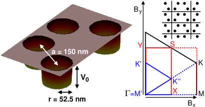
Figure 1: (Color online) Left: Rectangular unit cell in real space. Right: Orthorhombic irreducible Brillouin zone (rectangle $\Gamma XSY$) compared with the conventional one ($\Gamma MK$) for the honeycomb lattice. The basis vectors ${\bf B}_{x}$ and ${\bf B}_{y}$ are defined in the text. The hexagonal high symmetry points are ${\bf K}\equiv\frac{1}{3}{\bf B}_{y}={\bf K^{\prime}}$, ${\bf M}\equiv\boldsymbol{\Gamma}={\bf M^{\prime}}$. The mapping from the hexagonal to the orthorombic cell is performed as follows: the $\Gamma-M$ line corresponds to the $\Gamma-X-\Gamma$ path in the orthorhombic cell; the $M-K$ segment corresponds to $\Gamma-K^{\prime}$, and the $K-\Gamma$ segment corresponds to the two segment path $K^{\prime}-K^{\prime\prime}-M^{\prime}$, with ${\bf K^{\prime\prime}}\equiv\frac{1}{2}\left({\bf B}_{x}+\frac{1}{3}{\bf B}_{y}\right)$. Inset: part of the lattice in real space.

The electronic structure of the system was calculated with the Octopus package octopus . The code solves the Kohn-Sham equations on a real-space discrete grid. The only required convergence parameter is the grid spacing, and it is therefore not bound to any particular choice of a basis set. In order to describe a truly 2D distribution of atoms we follow the procedure described in Ref. cutoff , i.e., we impose a set of mixed boundary conditions (periodic in the plane, zero Dirichlet off-plane) and cut-off the Coulomb potential to zero along the direction perpendicular to the plane, while retaining its full long range of action within the plane. The levels obtained are rigorously equivalent to those calculated in an infinitely wide supercell in the direction perpendicular to the plane.

As shown in Fig. 1, the unit cell is chosen not to be minimal but to contain four dots, so that the 2D Bravais lattice becomes rectangular. The unit cell size is $\sim 130\,{\rm nm}\times\,225\,{\rm nm}$ and the grid spacing is $\sim 2.45\,{\rm nm}$. The reciprocal space cell is generated by the vectors ${\bf B}_{x}=\frac{2\pi}{a}\left[\frac{1}{3},0\right]$ and ${\bf B}_{y}=\frac{2\pi}{a}\left[0,\frac{1}{\sqrt{3}}\right]$, where $a$ is the interdot distance. The volume of this cell in reciprocal space is half the volume of the standard hexagonal BZ. Obviously, the physically meaningful results are not affected by our choice of the unit cell. However, in order to compare to calculations performed in the minimal (standard) cell, our bands must be appropriately unfolded. The high symmetry lines of the standard BZ can all be mapped to corresponding paths into the smaller BZ. The mapping is described in the caption of Fig. 1. For ease of comparison with previously published results, all the bands are displayed unfolded in this work. In the process of unfolding the band structure from the rectangular to the hexagonal cell, care must be exerted to avoid the phenomenon of aliasing, i.e., the spurious duplication of bands. This is greatly facilitated by the observation that the true bands must be continuous and differentiable at $K$ along the $\Gamma-K-M$ line.

As mentioned in the introduction, in order to assess the importance of e-e interactions, we compare the results for noninteracting electrons with those computed using the Kohn-Sham DFT approach dft within the 2D LDA. For the correlation part of the LDA we have used the parametrized form of the quantum Monte Carlo data calculated for the 2DEG by Attaccalite et al. attaccalite In view of previous works on QDs fabricated in the 2DEG reimann ; other we believe that the 2D-LDA provides a reasonable approximation for the energy bands considered here.

In Fig. 2 we show the energy bands calculated for noninteracting (a) and interacting electrons in the LDA (b) when $V_{0}=-0.6$ meV.

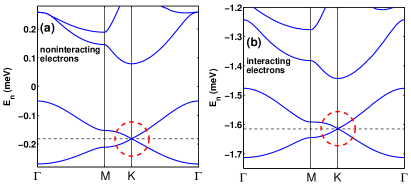
Figure 2: (Color online) Energy bands calculated for noninteracting (a) and interacting electrons ($N=1$ per dot) in density-functional theory (b). Clear Dirac points and a linear dispersion relation can be found in both cases (circles).

In both cases we find distinctive Dirac points at K with a linear dispersion relation. These are the defining attributes of graphene-like physics. From Fig. 2 it is clear that, in the case of singly occupied QDs in the AG, the e-e interactions do not make the Dirac point less stable. In general, the band structures are very similar, although, as expected, the e-e interactions reduce the bandwidth and thus increase the energy gaps between the two lowest bands. However, as an interesting exception to this tendency, the LDA result has a considerably smaller gap above the two lowest bands. We believe that this indicates the gap has a primarily kinetic origin, i.e. it arises from an overlap of neighboring localized orbitals forming a bonding-antibonding pair. Such a gap is reduced when the overlap of orbitals in the pair decreases, due to increased electron localization.

The general tendency of increased electron localization due to e-e interactions is clearly visible in the electron density shown in Fig. 3.

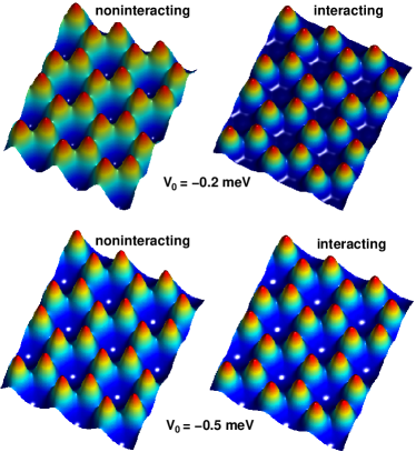
Figure 3: (Color online) Electron densities in artificial graphene ($N=1$ per dot) calculated for two depths of the potential wells, $V_{0}=-0.2$ meV (up) and $V_{0}=-0.5$ meV (down). The left and right panels show the results without and with the e-e interactions, respectively.

As expected, the relative difference in the density with and without e-e interactions is larger when $|V_{0}|$ is small. Indeed, for small $|V_{0}|$ the system is closer to the homogeneous 2DEG, where interactions (at small densities as in this case) drive the system to the Wigner crystal regime vignalebook .

To obtain a closer view on the stability of the Dirac points and the effects of e-e interactions, we next examine the onset and the size of the energy gap at the M point (see Fig. 2). The gap is defined as the energy difference between the Fermi level and the band closest to the Fermi level at the M point. Negative values correspond to crossings of the band(s) through the Fermi level, so that then there is no gap around the Dirac point. Figure 4 shows the size of the gap as a function of $|V_{0}|$, i.e., the depth of the QDs.

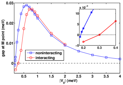
Figure 4: (Color online) Energy gap at the M point in the Brillouin zone as a function of the quantum-dot depth. Results without (squares) and with e-e interactions (circles) are shown for $N=1$ per dot. The inset shows a zoom of the regime where the gap opens.

In the absence of interactions the threshold potential for the gap is $V_{0}=-0.18$ meV which agrees perfectly with the tight-binding result in Ref. gibertini . When the interactions are included in the LDA level, the threshold shifts to $V_{0}=-0.30$ meV. In other words, the inclusion of e-e interactions leads us to predict that a deeper QDs is required in order to achieve an isolated Dirac point in the system. When $|V_{0}|$ is further increased the results without and with interactions become very similar. The gap reaches its maximum value at $V_{0}=-0.8$ meV (or $V_{0}=-0.6$ meV in the absence of interactions), which can be regarded as the optimal QD depth for the stability of the Dirac point. As expected, the gap shown in Fig. 4 closes asymptotically in the large-$|V_{0}|$ limit. The closing proceeds in a similar manner regardless of e-e interactions – albeit LDA results are not available at $|V_{0}|>2$ meV due to poor convergence. Gibertini et al. argued that there is a localization threshold in the system at $|V_{0}|\sim 3$ meV, due to the formation of disorder-induced bound states. This effect is not included in our calculations, since the perfect periodicity of the lattice keeps the wave functions extended, in principle up to the limit $|V_{0}|\rightarrow\infty$.

Finally we consider occupying the QDs with more than one electron. As suggested in Ref. gibertini , where a noninteracting tight-binding scheme was used, the next Dirac point should appear when $N=4$. In Fig. 5 we show the energy bands close to the Fermi energy when $N=4$ and $V_{0}=-2$ and -6.8 meV in the noninteracting (a) and interacting cases (b), respectively. The lowest two bands (not shown) are located at considerably lower energies, i.e., at about $-1.3$ and $-5.6$ meV, respectively. It is noteworthy that although the Dirac point can be found in both cases, it is much less stable in the interacting system: first, due to the strong intradot interactions the QDs need to be significantly deeper than without interactions. Furthermore, the Dirac point in the interacting case appears in an energy gap that is smaller by about an order of magnitude. Consequently, decreasing the potential depth from $|V_{0}|=6.8$ meV to 6.5 meV already disruptes the Dirac point, as the band above $E_{F}$ in Fig. 5(b) is shifted downwards. In contrast, the Dirac point in the noninteracting case is stable down to about $|V_{0}|=1$ meV. These results indicate that the realization of AG constitutes a challenge for the present engineering techniques if the QDs are occupied by several electrons.

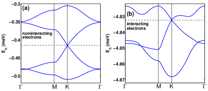
Figure 5: (Color online) Energy bands close to the Fermi energy calculated for noninteracting (a) and interacting electrons, when there are four electrons in each quantum dot. The two lowest bands (not shown) are located at about $-1.3$ and $-5.6$ meV in (a) and (b), respectively.

To summarize, we have studied the electronic properties of artificial graphene fabricated in the two-dimensional electron gas. The electron-electron interactions, treated here within the two-dimensional local-density approximation in density-functional theory, generally lead to stronger localization of the electrons in the quantum dots. The interactions shift the threshold for the emergence of isolated Dirac points to larger well depths than found without interactions. This effect is significantly pronounced when the number of electrons is increased. This sets a particular challenge for the realization of Dirac points if the quantum dots in the hexagonal lattice are occupied by more than a single electron.

- (1) For a review, see A. H. Castro Neto, F. Guinea, N. M. R. Peres, K. S. Novoselov, and A. K. Geim, Rev. Mod. Phys. 81, 109 (2009).
- (2) L. Tarruell, D. Greif, T. Uehlinger, G. Jotzu, and T. Esslinger, Nature 483, 302 (2012).
- (3) K. K. Gomes, W. Mar, W. Ko, F. Guinea, and H. C. Manoharan, Nature 483, 306 (2012).
- (4) C. Flindt, N. A. Mortensen, and A.-P. Jauho, Nano Lett. 5, 2515 (2005).
- (5) J. Pedersen, C. Flindt, N. A. Mortensen, and A.-P. Jauho, Phys. Rev. B 77, 045325 (2008).
- (6) C.-H. Park and S. G. Louie, Nano Lett. 9, 1793 (2009).
- (7) M. Gibertini, A. Singha, V. Pellegrini, M. Polini, G. Vignale, A. Pinczuk, L. N. Pfeiffer, and K. W. West, Phys. Rev. B 79, 241406(R) (2009).
- (8) G. de Simoni, A. Singha, M. Gibertini, B. Karmakar, M. Polini, V. Piazza, L. N. Pfeiffer, K. W. West, F. Beltram, and V. Pellegrini, Appl. Phys. Lett. 97, 132113 (2010).
- (9) A. Singha, M. Gibertini, B. Karmakar, S. Yuan, M. Polini, G. Vignale, M. I. Katsnelson, A. Pinczuk, L. N. Pfeiffer, K. W. West, and V. Pellegrini, Science 332, 1176 (2011).
- (10) Y. Barlas, T. Pereg-Barnea, M. Polini, R. Asgari, and A. H. MacDonald, Phys. Rev. Lett. 98, 236601 (2007).
- (11) E. H. Hwang, Ben Yu-Kuang Hu, and S. Das Sarma, Phys. Rev. Lett. 99, 226801 (2007).
- (12) M. Polini, R.Asgari, G. Borghi, Y. Barlas, T. Pereg-Barnea, and A. H. MacDonald, Phys. Rev. B 77, 081411(R) (2008).
- (13) L. Nadvornik, M. Orlita, N. A. Goncharuk, L. Smrcka, V. Novak, V. Jurka, K. Hruska, Z. Vyborny, Z. R. Wasilewski, M. Potemski, and K. Vyborny, New. J. Phys. (in print), arXiv:1104.5427.
- (14) Y. Zhang and C. Zhang, Phys. Rev. B 84, 085123 (2011).
- (15) R. M. Dreizler and E. K. U. Gross, Density Functional Theory (Springer, Berlin, 1990); J. P. Perdew and S. Kurth, in A Primer in Density Functional Theory, Lecture Notes in Physics Vol. 620, edited by C. Fiolhais, F. Nogueira, and M. Marques (Springer, Berlin, 2003).
- (16) S. M. Reimann and M. Manninen, Rev. Mod. Phys. 74, 1283 (2002).
- (17) For recent works, see, e.g., M. C. Rogge, E. Räsänen, and R. J. Haug, Phys. Rev. Lett. 105, 046802 (2010); E. Räsänen, H. Saarikoski, A. Harju, M. Ciorga, and A. S. Sachrajda, Phys. Rev. B 77, 041302(R) (2008).
- (18) L. P. Kouwenhoven, D. G. Austing, and S. Tarucha, Rep. Prog. Phys. 64, 701 (2001).
- (19) C. F. Hirjibehedin, A. Pinczuk, B. S. Dennis, L. N. Pfeiffer, and K. W. West, Phys. Rev. B 65, 161309(R) (2002).
- (20) C. F. Hirjibehedin, I. Dujovne, A. Pinczuk, B. S. Dennis, L. N. Pfeiffer, and K. W. West, Phys. Rev. Lett. 95, 066803 (2005).
- (21) C.P. Garcia et al., Phys. Rev. Lett. 95, 266806 2005).
- (22) M. A. L. Marques, A. Castro, G. F. Bertsch, A. Rubio, Comput. Phys. Commun. 151, 60 (2003); A. Castro, H. Appel, M. Oliveira, C. A. Rozzi, X. Andrade, F. Lorenzen, M. A. L. Marques, E. K. U. Gross, and A. Rubio, Phys. Stat. Sol. (b) 243, 2465 (2006).
- (23) A. Castro, E. Räsänen, and C. A. Rozzi, Phys. Rev. B 80, 033102 (2009).
- (24) C. Attaccalite, S. Moroni, P. Gori-Giorgi, and G. B. Bachelet, Phys. Rev. Lett. 88, 256601 (2002).
- (25) G. F. Giuliani and G. Vignale, in Quantum Theory of the Electron Liquid, (Cambridge University Press, Cambridge, 2005).