Resonant charge transfer at dielectric surfaces

Abstract

We report on the theoretical description of secondary electron emission due to resonant charge transfer occurring during the collision of metastable $\mathrm{N_{2}}(^{3}\Sigma_{u}^{+})$ molecules with dielectric surfaces. The emission is described as a two step process consisting of electron capture to form an intermediate shape resonance $\mathrm{N_{2}^{-}}(^{2}\Pi_{g})$ and subsequent electron emission by decay of this ion, either due to its natural life time or its interaction with the surface. The electron capture is modeled using the Keldysh Green’s function technique and the negative ion decay is described by a combination of the Keldysh technique and a rate equation approach. We find the resonant capture of electrons to be very efficient and the natural decay to be clearly dominating over the surface-induced decay. Secondary electron emission coefficients are calculated for Al₂O₃, MgO, SiO₂, and diamond at several kinetic energies of the projectile. With the exception of MgO the coefficients turn out to be of the order of $10^{-1}$ over the whole range of kinetic energies. This rather large value is a direct consequence of the shape resonance acting as a relay state for electron emission.

1 Introduction

Secondary electron emission from dielectric surfaces due to various projectiles is a fundamental process of great technological significance. The associated electron yield is usually represented by the secondary electron emission coefficient $\gamma_{e}$ which denotes the average number of electrons released by a single collision of a particular type. Thus, $\gamma_{e}$ is specific to the surface material, the projectile, and the particular collision process under consideration.

To illustrate the importance of secondary electron emission from dielectric materials we first consider an atmospheric pressure dielectric barrier discharge (DBD). Various technological processes like polymer surface treatment, thin film coating, sterilization, gas flow control and ozone production Massines2008Recent ; Golubovskii2002Influence are based on this type of discharge. All of these are sensitive to the discharge’s stability and homogeneity. Secondary electron emission from the electrodes increases the DBD’s self-sustain and is thus crucial to the discharge’s operation mode. In particular, there is some evidence that the stability of DBDs is controlled by secondary electron emission from plasma boundaries by impacting metastable species Brandenburg2005Diffuse . Although DBDs have been studied for more than 20 years, their basic mechanism is still not entirely understood Massines2008Recent . To overcome this deficiency numerical investigations are inevitable Golubovskii2002Influence ; Brandenburg2005Diffuse . These studies require $\gamma_{e}$ as an input parameter, which either has to be measured experimentally or calculated from first principles.

Another application are plasma display panels (PDPs), which are used in large size TV monitors. PDPs are usually based on AC driven high pressure microdischarges Punset1998Twodimensional in noble gas mixtures Auday2000Secondary and often employ electrodes coated with Al₂O₃ or MgO Vink2002Materials . The panel’s firing voltage, that is, the voltage required for discharging, is directly influenced by secondary electron emission from the dielectric electrodes Vink2002Materials , for instance, due to impacting metastable species. In order to improve the performance of PDPs, theoretical investigations of the employed materials, the overall discharge geometry, and the operation mode are necessary Punset1998Twodimensional . These studies again require the emission coefficient $\gamma_{e}$ as an input parameter.

The demand for reliable $\gamma_{e}$ data for use in numerical simulations of PDPs, DBDs, and related gas discharges contrasts with the very sparse and often uncertain available reference data. In many cases rules of the thumb have to be used Raizer91 . Especially sparse is the data base for secondary electron emission due to metastable molecules. The objective of the present work is therefore to contribute to the filling of this particular gap. We aim to establish a model that allows for easy calculation of the secondary electron emission coefficient due to impacting metastable molecules on dielectric surfaces, taking $\mathrm{N_{2}}(^{3}\Sigma_{u}^{+})$ as an example. Other projectile-surface combinations can be modelled in the same spirit.

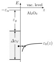
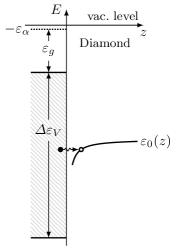
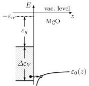
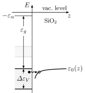
Figure 1: Energetic structure of the different dielectric materials considered in this work characterized by the electron affinity $\varepsilon_{\alpha}$, the size of the energy gap $\varepsilon_{g}$, and the width of the valence band $\Delta\varepsilon_{V}$. For SiO₂ the energetically blocked upper valence band is marked in shaded grey. Also indicated is the variation of the molecular hole level with distance. For an explanation of the molecular image shift see Sec. 2.1. Note that the figure is to scale in terms of energy units.

The model we propose is an effective one, stripped of some of the microscopic details of the system and characterized by a small number of material specific parameters instead. In a previous work Marbach2011Auger we presented such a model for the case of Auger de-excitation of $\mathrm{N_{2}}(^{3}\Sigma_{u}^{+})$ on aluminum, corresponding to the reaction

$$\mathrm{N_{2}}(^{3}\Sigma_{u}^{+})+e_{\vec{k}}\xrightarrow{\mathrm{Auger}}\mathrm{N_{2}}(^{1}\Sigma_{g}^{+})+e_{\vec{q}}\;,$$ (1)

with $e_{\vec{k}}$ and $e_{\vec{q}}$ denoting an electron within the surface and a free electron, respectively. Another important process capable of generating secondary electrons by impact of $\mathrm{N_{2}}(^{3}\Sigma_{u}^{+})$ is the combination of electron capture by resonant charge transfer (RCT) to form the $\mathrm{N_{2}^{-}}(^{2}\Pi_{g})$ shape resonance and subsequent decay of the intermediate ion, corresponding to

$$\mathrm{N_{2}}(^{3}\Sigma_{u}^{+})+e_{\vec{k}}\xrightarrow{\mathrm{RCT}}\mathrm{N_{2}^{-}}(^{2}\Pi_{g})\xrightarrow{\mathrm{RCT}}\mathrm{N_{2}}(^{1}\Sigma_{g}^{+})+e_{\vec{q}}\;.$$ (2)

Except for diamond, the Auger channel (1) is energetically suppressed for all of the dielectric materials considered in this work whereas the RCT channel (2) is energetically always possible (see Fig. 1). Hence, we focus on the resonant reaction (2) which was also found to be very efficient when $\mathrm{N_{2}}(^{3}\Sigma_{u}^{+})$ collides with a metallic surface Lorente1999N2 ; Stracke1998Formation . In order to describe this process, we will use a generalization of the model presented in Marbach2011Auger and apply it to dielectric surfaces. Since the adaption is straightforward we only give a brief sketch of the model and refer the reader to Marbach2011Auger for details.

The solid surface is treated as a potential well with a depth

$$V_{0}=-\varepsilon_{\alpha}-\varepsilon_{g}-\Delta\varepsilon_{V}\;,$$ (3)

filled up to the top of the valence band

$$\varepsilon_{V}=-\varepsilon_{\alpha}-\varepsilon_{g}\;.$$ (4)

Here $\varepsilon_{\alpha}$, $\varepsilon_{g}$ and $\Delta\varepsilon_{V}$ denote the solid’s electron affinity, its energy gap and the width of its valence band, respectively. The wave functions of such a potential well are easily calculated and may be found in Marbach2011Auger . The particular electronic parameters of the dielectric materials investigated in this work Yeo2002Metaldielectric ; Ciraci1983Electronic ; Robertson2006High ; Rutter1998Ab ; Robertson2006Band ; Bhagavantam1948Dielectric ; Kim2008Electron ; Tobita2008Electronic ; Fontanella1974Lowfrequency ; Schreiber2002Monte ; Ciraci1982Surface are summarized in Table 1.

The molecule is characterized by a two level system consisting of an initially empty ground state level $0$ and an initially filled excited level $1$. The molecular wave functions associated with these two levels are calculated from a LCAO combination of atomic nitrogen wave functions, identifying $0$ and $1$ with the $2\pi_{u}$ and $2\pi_{g}$ molecular orbitals Marbach2011Auger . The ionization energies $\varepsilon_{0/1}^{\infty}$ of the two levels Kaldor1984Generalmodelspace ; Honigmann2006Complex are listed in Table 2 for the unperturbed molecule. As will be shown in Sec. 2.1, both of these levels shift downwards upon approaching the surface, provided that only the RCT channel (2) is considered.

We will describe the resonant reaction (2) as a two-step process. First, we will employ the Keldysh Green’s function technique to model the resonant electron capture into the initially vacant ground state level $0$. This step of the process is depicted in Fig. 1. The second step consists of resonant electron emission by decay of the intermediate negative ion. The decay can be due to the ion-surface coupling, which is mediated by the image interaction, or due to the ions natural life time, that is, due to auto-decay. Considering a $\mathrm{N_{2}^{-}}(^{2}\Pi_{g})$ ion colliding with the surface we will model the surface-induced decay again by a Keldysh approach, the auto-decay, however, by a rate equation approach. Electron capture and release we will be coupled by a rate equation scheme that is based on a conditional decay reaction.

The outline of the remainder of this article is as follows. In Sec. 2 we will setup the quantum mechanical model of the molecular electron-capture and conduct a quantum-kinetic calculation on top of it. The treatment of surface-induced decay and auto-decay as well as their coupling to the initial electron capture will be presented in Section 3. Finally, we show and discuss numerical results for selected surfaces in Sec. 4 and give a conclusion in Sec. 5.

2 Resonant electron capture

	$\boldsymbol{\varepsilon_{\alpha}\,\,[eV]}$	$\boldsymbol{\varepsilon_{g}\,\,[eV]}$	$\boldsymbol{\Delta\varepsilon_{V}\,\,[eV]}$	$\boldsymbol{\varepsilon_{r}^{b}}$
Al2O3	1.0 Yeo2002Metaldielectric	8.7 Ciraci1983Electronic	11.8 Ciraci1983Electronic	9.0 Robertson2006High
diamond	$0.52$ Rutter1998Ab	5.48 Robertson2006Band	21.0 Robertson2006Band	5.66 Bhagavantam1948Dielectric
MgO	$0.925$ Kim2008Electron	7.6 Tobita2008Electronic	8.5 Tobita2008Electronic	9.83 Fontanella1974Lowfrequency
SiO2	$0.9$ Schreiber2002Monte	$13.8$ Ciraci1982Surface	$5.3$ Ciraci1982Surface	$3.9$ Robertson2006High

Table 1: Electronic parameters for the dielectric materials considered in this work: electron affinity $\varepsilon_{\alpha}$, energy gap $\varepsilon_{g}$, valence band width $\Delta\varepsilon_{V}$, and static relative dielectric constant $\varepsilon_{r}^{b}$. The electron affinity of diamond and MgO is calculated from a mean value due to lack of consistent data. Note, for SiO₂ only the lower valence band is considered. The upper valence band starts at $8.9\,eV$ and has a width of $2.7\,eV$ Ciraci1982Surface . It is thus energetically well separated from the molecular vacancy level $\varepsilon_{0}$ and does therefore not contribute to the electron capture.

2.1 Model

The molecule-surface system is described by the following Hamiltonian

$$\begin{split}H(t)&=\sum_{\vec{k}}\varepsilon_{\vec{k}}^{{\phantom{{\dagger}}}}\,c_{\vec{k}}^{{\dagger}}\,c_{\vec{k}}^{{\phantom{{\dagger}}}}+\varepsilon_{0}^{{\phantom{{\dagger}}}}(t)\,c_{0}^{{\dagger}}\,c_{0}^{{\phantom{{\dagger}}}}\\ &\phantom{=}+\sum_{\vec{k}}\left(V_{\vec{k}}^{{\phantom{{*}}}\!}(t)\,c_{\vec{k}}^{{\dagger}}\,c_{0}^{{\phantom{{\dagger}}}}+V_{\vec{k}}^{*}(t)\,c_{\vec{k}}^{{\phantom{{\dagger}}}}\,c_{0}^{{\dagger}}\right)\;,\end{split}$$ (5)

where $\vec{k}$ denotes electronic states within the solid’s valence band and $0$ labels the molecule’s ground state level, which is initially empty. Since we are considering the capture of an additional electron by the metastable state $\mathrm{N_{2}}(^{3}\Sigma_{u}^{+})$, the level $0$ equals the lower ionization level of $\mathrm{N_{2}^{-}}(^{2}\Pi_{g})$.

To understand the variation of $\varepsilon_{0}$ with time we follow Newns1983Charge and consider a negative nitrogen ion situated at a distance $z_{R}$ from a dielectric surface, the relative static permittivity of which we denote by $\varepsilon_{r}^{b}$. Since the ion is negatively charged its overall energy is lowered by the value of the image potential at $z_{R}$, for which we use the classical expression (see however below)

$$V_{i}(z_{R})\approx-\frac{\varepsilon_{r}^{b}-1}{\varepsilon_{r}^{b}+1}\frac{e^{2}}{4\pi\varepsilon_{0}}\frac{1}{4z_{R}}\;.$$ (6)

In order to obtain the effective ionization energy $\varepsilon_{0}(z_{R})$, we virtually move the negative ion from the position $z_{R}$ to a point infinitely far away from the surface, ionize the electron bound in the $0$ state to the vacuum level, and relocate the resulting neutral molecule back to the original distance $z_{R}$. The net energy change during this process determines the effective ionization energy

$$\varepsilon_{0}(z_{R}) =-\Delta\varepsilon=-\bigl{[}\;\underbrace{-V_{i}(z_{R})}_{N_{2}^{-}\rightarrow\infty}+\underbrace{(-\varepsilon_{0}^{\infty})}_{N_{2}^{-}\rightarrow N_{2}}+\underbrace{0}_{N_{2}\rightarrow z_{R}}\bigr{]}$$ (7a)

$$=\varepsilon_{0}^{\infty}+V_{i}(z_{R})\;.$$ (7b)

Since this procedure is independent of the specific molecular level, we conclude that upon approaching the surface each and any of the negative ion’s ionization levels shifts downwards. The reader may note that the decrease of the ionization energies does not correspond to an actual energy change of the negative ion. The ionization levels are defined solely in terms of the removal of an electron from the molecule and, thus, do not imply an energy change for a bound electron.

Employing the usual trajectory approximation Hagstrum1954Theory together with the trajectory

$$\vec{R}(t)=z_{R}(t)\,\vec{e}_{z}=\left(v_{0}\left|t\right|+z_{0}\right)\vec{e}_{z}\;,$$ (8)

the relation (7b) can also be understood as $\varepsilon_{0}(t)$.

	$\boldsymbol{\mathrm{N_{2}}(^{1}\Sigma_{g}^{+})\,\,[eV]}$	$\boldsymbol{\mathrm{N_{2}}(^{3}\Sigma_{u}^{+})\,\,[eV]}$	$\boldsymbol{\mathrm{N_{2}^{-}}(^{2}\Pi_{g})\,\,[eV]}$
$\varepsilon_{0}^{\infty}$	$-17.25$ Kaldor1984Generalmodelspace	–	$-14.49$ Honigmann2006Complex
$\varepsilon_{1}^{\infty}$	–	$-9.67$ Kaldor1984Generalmodelspace	$1.18$ Honigmann2006Complex

Table 2: Ionization energies of the molecular ground state level $0$ and the excited level $1$ for a free nitrogen molecule in its ground state $\mathrm{N_{2}}(^{1}\Sigma_{g}^{+})$ and its metastable state $\mathrm{N_{2}}(^{3}\Sigma_{u}^{+})$ as well as for the negative ion shape resonance $\mathrm{N_{2}^{-}}(^{2}\Pi_{g})$.

Generalizing Gadzuk’s Gadzuk1967Theory1 treatment of mono-nuclear projectiles to bi-nuclear projectiles, the tunnelling matrix element $V_{\vec{k}}$ is given by

$$\begin{split}V_{\vec{k}}(t)=&\int\mathrm{d}\vec{r}\;\Psi_{\vec{k}}^{{*}}(\vec{r}\hskip 1.00006pt)\bigl{[}V_{M}(\vec{r},t)+V_{SM}(z)\bigr{]}\,\Psi_{0}^{{\phantom{{*}}}}(\vec{r}_{\varphi}(t))\;,\end{split}$$ (9)

where the time dependence arises from the molecule’s motion and $\vec{r}_{\varphi}$ equals the vector $\vec{r}$ as seen from the molecular reference frame, that is,

$$\vec{r}_{\varphi}(t)=\hat{\Omega}(\varphi)\left[\vec{r}-\vec{R}(t)\right]\;,$$ (10)

with an appropriate rotation matrix $\hat{\Omega}(\varphi)$ Marbach2011Auger .

The expression $V_{M}$ specifies the Coulomb potential of the screened molecular nuclei Gadzuk1967Theory1

$$\begin{split}V_{M}(\vec{r},t)=&-\frac{Z_{\text{eff}}\,e^{2}}{4\pi\varepsilon_{0}\,\varepsilon_{r}(z)}\left[\frac{1}{|\vec{r}-\vec{R}_{1}(t)|}+\frac{1}{|\vec{r}-\vec{R}_{2}(t)|}\right]\;,\end{split}$$ (11)

with $Z_{\text{eff}}\approx 4$ Marbach2011Auger and

$$\vec{R}_{1/2}(t)=\vec{R}\pm\frac{\vec{\varrho}}{2}$$ (12)

denoting the positions of the two nuclei, which are given in terms of the center of mass coordinate $\vec{R}$ and the inter-nuclear vector →ϱ. The static dielectric constant $\varepsilon_{r}(z)$ is approximated by

$$\varepsilon_{r}(z)=\begin{cases}\varepsilon_{r}^{b}&,\,z\leq 0\\ 1&,\,z>0\end{cases}\;.$$ (13)

The term $V_{SM}$ labels the electron’s self image interaction potential Gadzuk1967Theory1

$$\begin{split}V_{SM}(z)=&\;\Theta(z)\bigl{[}\Theta(z_{c}-z)V_{0}+\Theta(z-z_{c})V_{i}(z)\bigr{]}\;.\end{split}$$ (14)

Here we have used the usual truncation of the classical image potential close to the surface Kurpick1996Basic with

$$V_{i}(z_{c})\stackrel{{\scriptstyle!}}{{=}}V_{0}\;.$$ (15)

The wave functions of the metal electron $\Psi_{\vec{k}}$ and the one of the molecular electron $\Psi_{0}$ are taken from Marbach2011Auger . We treat the magnetic quantum number $m$, which is introduced within the LCAO representation of the molecular wave functions Marbach2011Auger , as an external parameter.

2.2 Quantum kinetics

The Hamiltonian (5) describes a standard problem of many particle physics. It can be treated exactly using the Keldysh technique Blandin1976Localized . The self-energy solely consists of a first order retarded and advanced term

$$\Sigma_{\vec{k}0}^{R/A}(t_{1},t_{2}) =\frac{i}{\hbar}V_{\vec{k}}(t_{1})\,\delta(t_{1}-t_{2})$$ (16a)

$$=-\left[\Sigma_{0\vec{k}}^{R/A}(t_{1},t_{2})\right]^{*}\;.$$ (16b)

The Keldysh component of the self-energy vanishes, the Dyson equation for the Keldysh Green’s function can thus be solved to give

$$\begin{split}G_{\alpha\beta}^{K}(t,t^{\prime})&=-i\sum_{\gamma}\bigl{[}1-2n_{\gamma}(t_{0})\bigr{]}\\ &\phantom{=}\times G_{\alpha\gamma}^{R}(t,t_{0})\,G_{\gamma\beta}^{A}(t_{0},t^{\prime})\;,\end{split}$$ (17)

where $\alpha$ and $\beta$ can take the values $0$ or $\vec{k}$ and $\gamma$ runs over all states $\{0,\vec{k}\}$ of the system. Note that $t_{0}$ is shorthand for $-\infty$. Equation (17) can be used to calculate the occupation of the molecular level

$$n_{0}(t) =\frac{1}{2}\left[1-iG_{00}^{K}(t,t)\right]$$ (18a)

$$=\sum_{\vec{k}}n_{\vec{k}}(t_{0})\,|G_{0\vec{k}}^{R}(t,t_{0})|^{2}\;,$$ (18b)

where we have used the relation Blandin1976Localized ; Mii1996Interpolation

$$\sum_{\gamma}G_{\alpha\gamma}^{R}(t,t_{0})\,G_{\gamma\alpha}^{A}(t_{0},t)=1\;.$$ (19)

Evaluation of the Green’s function $G_{0\vec{k}}^{R}$ appearing in (18b) requires knowledge of the diagonal component $G_{00}^{R}$, the Dyson equation of which can be solved iteratively to yield

$$\begin{split}&G_{00}^{R{\phantom{(}\!}}(t,t^{\prime})=G_{00}^{R{(0)\!}}(t,t^{\prime})\,\sigma_{0}(t,t^{\prime})\;,\end{split}$$ (20)

with

$$G_{00}^{R{(0)\!}}(t,t^{\prime})=-i\Theta(t-t^{\prime})\,e^{-\frac{i}{\hbar}\int_{t^{\prime}}^{t_{\phantom{1}}}\mathrm{d}t_{1}\;\varepsilon_{0}(t_{1})}\;,$$ (21)

and $\sigma_{0}$ given by the infinite series

$$\begin{split}&\sigma_{0}(t,t^{\prime})=1-\int_{t^{\prime}}^{t_{\phantom{1}}}\mathrm{d}t_{1}\int_{t^{\prime}}^{t_{1}}\mathrm{d}t_{2}\;\Delta_{0}(t_{1},t_{2})\\ &\quad+\int_{t^{\prime}}^{t_{\phantom{1}}}\mathrm{d}t_{1}\int_{t^{\prime}}^{t_{1}}\mathrm{d}t_{2}\int_{t^{\prime}}^{t_{2}}\mathrm{d}t_{3}\int_{t^{\prime}}^{t_{3}}\mathrm{d}t_{4}\;\Delta_{0}(t_{1},t_{2})\,\Delta_{0}(t_{3},t_{4})\\ &\quad-\dots\;.\end{split}$$ (22)

The quantity $\Delta_{0}$ emerges from the self-energy and reads

$$\begin{split}\Delta_{0}(t_{1},t_{2})&=\frac{1}{\hbar^{2}}\sum_{\vec{k}}V_{\vec{k}}^{*}(t_{1})\,V_{\vec{k}}(t_{2})\\ &\phantom{=}\times e^{-\frac{i}{\hbar}\varepsilon_{\vec{k}}(t_{1}-t_{2})}\,e^{-\frac{i}{\hbar}\int_{t_{1}}^{t_{2}}\!\mathrm{d}\bar{t}\,\varepsilon_{0}(\bar{t})}\;.\end{split}$$ (23)

By employing now the Dyson equation for $G_{0\vec{k}}^{R}$, with the self energy (16b), the occupancy of the molecular level (18b) can be written as

$$\begin{split}n_{0}(t)&=\int_{t_{0}}^{t_{\phantom{1}}}\mathrm{d}t_{1}\int_{t_{0}}^{t_{\phantom{1}}}\mathrm{d}t_{2}\;\widetilde{\Delta}_{0}(t_{1},t_{2})\,\sigma_{0}(t,t_{1})\,\sigma_{0}^{*}(t,t_{2})\;.\end{split}$$ (24)

Here $\widetilde{\Delta}_{0}$ is equal to $\Delta_{0}$ with an additional factor $n_{\vec{k}}(t_{0})$ under the $\vec{k}$ sum. In general this subtlety would deny further simplification of Eq. (24). However, since for a dielectric surface the active energy band is the valence band, which is completely filled, the terms $\Delta_{0}$ and $\widetilde{\Delta}_{0}$ are essentially the same. Note that even for metallic surfaces with an incompletely filled conduction band these terms will still be almost equal, as long as the molecular resonance stays inside the occupied portion of the band.

To simplify Eq. (24), we first note that when $t$ is kept constant the derivative of Eq. (22) with respect to $t^{\prime}$ can be shown to read

$$\frac{\partial\sigma_{0}(t,t^{\prime})}{\partial t^{\prime}}=\int_{t^{\prime}}^{t_{\phantom{1}}}\mathrm{d}\bar{t}\;\sigma_{0}(t,\bar{t})\,\Delta_{0}(\bar{t},t^{\prime})\;.$$ (25)

Using this expression we can now rewrite (24) into

$$n_{0}(t) =2\Re\left[\int_{t_{0}}^{t_{\phantom{1}}}\mathrm{d}t_{2}\;\sigma_{0}^{*}(t,t_{2})\frac{\mathrm{d}\sigma_{0}(t,t_{2})}{\mathrm{d}t_{2}}\right]$$ (26a)

$$\begin{split}&=2\bigl{[}1-\sigma_{0}(t,t_{0})\,\sigma_{0}^{*}(t,t_{0})\bigr{]}\\ &\phantom{=}-2\Re\left[\int_{t_{0}}^{t_{\phantom{1}}}\mathrm{d}t_{2}\;\sigma_{0}(t,t_{2})\frac{\mathrm{d}\sigma_{0}^{*}(t,t_{2})}{\mathrm{d}t_{2}}\right]\;,\end{split}$$ (26b)

where we have used integration by parts in the last line. Combining (26a) and (26b), we obtain

$$n_{0}(t)=1-\sigma_{0}(t,t_{0})\,\sigma_{0}^{*}(t,t_{0})\;.$$ (27)

We have not yet used any approximation to $\sigma_{0}$. The result (27) is thus exact. Since $V_{\vec{k}}$ is small it is however sufficient to approximately re-sum the infinite series (22). Using the exponential re-summation technique described in Marbach2011Auger and retaining only the lowest order term we obtain

$$\begin{split}\sigma_{0}(t,t^{\prime})\approx e^{-\int_{t^{\prime}}^{t_{\phantom{1}}}\mathrm{d}t_{1}\int_{t^{\prime}}^{t_{1}}\mathrm{d}t_{2}\;\Delta_{0}(t_{1},t_{2})}\;,\end{split}$$ (28)

which after insertion into (27) yields

$$n_{0}(t)\approx 1-e^{-\int_{t_{0}}^{t_{\phantom{1}}}\mathrm{d}t_{1}\int_{t_{0}}^{t_{\phantom{1}}}\mathrm{d}t_{2}\;\Delta_{0}(t_{1},t_{2})}\;.$$ (29)

Evaluating (29) at $t=t_{0}$ we see that the initial condition $n_{0}(t_{0})=0$ is fulfilled. Taking the limit $L\rightarrow\infty$ within the metallic wave function Marbach2011Auger , the $\vec{k}$ sum in (23) turns into an integral. For a numerical treatment it is convenient to exchange the $\vec{k}$ and $t_{1/2}$ integrations in (29). The integral in the exponent of (29) then takes the form

$$\begin{split}\int_{t_{0}}^{t_{\phantom{1}}}\mathrm{d}t_{1}\int_{t_{0}}^{t_{\phantom{1}}}\mathrm{d}t_{2}\;\Delta_{0}(t_{1},t_{2})&=\frac{L^{3}}{2\hbar^{2}(2\pi)^{3}}\int\!\mathrm{d}\vec{k}\;\left|\Lambda_{0}(\vec{k},t)\right|^{2}\;\end{split}$$ (30)

with

$$\begin{split}\Lambda_{0}(\vec{k},t)=\int_{t_{0}}^{t_{\phantom{1}}}\mathrm{d}t_{1}\;V_{\vec{k}}(t_{1})\,e^{\frac{i}{\hbar}\varepsilon_{\vec{k}}t_{1}}\,e^{\frac{i}{\hbar}\int_{0}^{t_{1}}\!\mathrm{d}t_{2}\,\varepsilon_{0}(t_{2})}\;,\end{split}$$ (31)

where the $L^{3}$ factor in (30) cancels with the $L^{-3/2}$ factor in $V_{\vec{k}}$.

2.3 Matrix element separation

In order to make a numerical calculation of the ground state level’s occupancy feasible, we need to introduce approximations to the matrix element.

Numerical evaluation of the full matrix element (9) suggests that $V_{M}$ is clearly dominating over $V_{SM}$ and that in addition the matrix element may be neglected in the half space $z\leq 0$. Making use of these findings we can separate the matrix element’s time dependence by performing the coordinate transformation

$$\vec{r}=\underbrace{\hat{\Omega}^{\dagger}(\varphi)\,\vec{r}_{\varphi}}_{\vec{r}_{\varphi}^{\,{\prime}}}+\vec{R}(t)\;,$$ (32)

which is the inverse of (10). Utilizing the relation

$$|\vec{r}-\vec{R}_{1/2}(t)| =|\vec{r}-\vec{R}(t)\mp\frac{\varrho}{2}\,\hat{\Omega}^{\dagger}(\varphi)\,\vec{e}_{z}|$$ (33a)

$$=|\hat{\Omega}^{\dagger}(\varphi)[\vec{r}_{\varphi}\mp\frac{\varrho}{2}\,\vec{e}_{z}]|$$ (33b)

$$=|\vec{r}_{\varphi}\mp\frac{\varrho}{2}\,\vec{e}_{z}|\;$$ (33c)

and approximating $\Theta(z^{\prime}_{\varphi}+z_{R}(t))$ by $\Theta(z^{\prime}_{\varphi}+z_{0})$ as in Marbach2011Auger we then obtain

$$V_{\vec{k}}(t)\approx C\,T_{k_{z}}^{*}e^{-\varkappa_{k_{z}}z_{R}(t)}\widetilde{V}_{\vec{k}}\;,$$ (34)

where $T_{k_{z}}$ is defined in Marbach2011Auger ,

$$C =\frac{mN_{k}}{\sqrt{2\pi N_{2\pi_{u}}\varkappa}}\frac{Z_{\text{eff}}\,e^{2}}{4\pi\varepsilon_{0}}\;,{\rm and}$$ (35a)

$$\begin{split}\widetilde{V}_{\vec{k}}&=\int\mathrm{d}\vec{r}_{\varphi}\;\Theta(z_{\varphi}^{\prime}-z_{0})\,e^{-\varkappa_{k_{z}}z_{\varphi}^{\prime}}\left[\frac{1}{r_{\varphi}^{+}}+\frac{1}{r_{\varphi}^{-}}\right]\\ &\phantom{=}\times\left[e^{-r_{\varphi}^{+}}+e^{-r_{\varphi}^{-}}\right](x_{\varphi}+imy_{\varphi})\\ &\phantom{=}\times e^{-i\left(k_{x}x_{\varphi}^{\prime}+k_{y}y_{\varphi}^{\prime}\right)}\;.\end{split}$$ (35b)

Here we have rescaled $\vec{r}_{\varphi}$, $\vec{k}$ and $t$ according to

$$\vec{r}_{\varphi}\rightarrow\frac{1}{\varkappa}\vec{r}_{\varphi}\;,\qquad\vec{k}\rightarrow\varkappa\vec{k}\;,\qquad t\rightarrow\frac{1}{\varkappa v_{0}}t\;,$$ (36)

with $\varkappa=\frac{Z_{\text{eff}}}{2\,a_{B}}$. Furthermore, the expressions $r_{\varphi}^{\pm}$ are shorthand notation for

$$r_{\varphi}^{\pm}=\left|\vec{r}_{\varphi}\pm\frac{\varrho}{2}\,\vec{e}_{z^{\prime}}\right|\;.$$ (37)

Inserting (34) into Eq. (31) yields

$$\begin{split}\Lambda(\vec{k},t)&=\frac{C_{m}\,T_{k_{z}}^{*}\widetilde{V}_{\vec{k}}}{\varkappa v_{0}}\int_{t_{0}}^{t_{\phantom{1}}}\mathrm{d}t_{1}\;e^{-\varkappa_{k_{z}}z_{R}(t)}\,e^{\frac{i}{\hbar\varkappa v_{0}}\varepsilon_{\vec{k}}t_{1}}\\ &\phantom{=}\times e^{\frac{i}{\hbar\varkappa v_{0}}\int_{0}^{t_{1}}\!\mathrm{d}t_{2}\,\varepsilon_{0}(t_{2})}\;,\end{split}$$ (38)

which enables us to calculate the involved space and time integrals independently within a numerical simulation.

3 Decay of the negative ion

3.1 Surface-induced decay

The surface-induced decay reaction can be described by the Hamiltonian

$$\begin{split}H(t)=&\sum_{\vec{q}}\varepsilon_{\vec{q}}^{{\phantom{{\dagger}}}}(t)\,c_{\vec{q}}^{{\dagger}}\,c_{\vec{q}}^{{\phantom{{\dagger}}}}+\varepsilon_{1}^{{\phantom{{\dagger}}}}(t)\,c_{1}^{{\dagger}}\,c_{1}^{{\phantom{{\dagger}}}}\\ &+\sum_{\vec{q}}\left(V_{\vec{q}}^{{\phantom{{*}}}\!}(t)\,c_{\vec{q}}^{{\dagger}}\,c_{1}^{{\phantom{{\dagger}}}}+V_{\vec{q}}^{*}(t)\,c_{\vec{q}}^{{\phantom{{\dagger}}}}\,c_{1}^{{\dagger}}\right)\;,\end{split}$$ (39)

which is structurally identical to the resonant capture Hamiltonian (5) with the associations $\vec{k}\leftrightarrow\vec{q}$ and $0\leftrightarrow 1$.

In (39) $\varepsilon_{1}$ is the upper ionization level of the negative nitrogen ion and $\varepsilon_{\vec{q}}$ denotes the energy of the free electron states, which are centered around the moving molecule. Both of these energy levels shift downwards upon approaching the surface, as can be shown using the analysis presented in Sec. 2.1

$$\varepsilon_{1}(t) =\varepsilon_{1}^{\infty}+V_{i}(z_{R}(t))\;,$$ (40a)

$$\varepsilon_{\vec{q}}(t) =\varepsilon_{\vec{q}}^{\infty}+V_{i}(z_{R}(t))\;.$$ (40b)

This fact implies that the difference $\varepsilon_{1}(t)-\varepsilon_{\vec{q}}(t)$ is constant in time.

The tunnelling matrix element $V_{\vec{q}}$ is given by

$$\begin{split}V_{\vec{q}}(t)&=\alpha(\varepsilon_{q_{z}}^{\infty},t)\int\mathrm{d}\vec{r}\;\Psi_{\vec{q}_{\varphi}}^{{*}}(\vec{r}_{\varphi}(t))\,\Psi_{1}^{{\phantom{{*}}}}(\vec{r}_{\varphi}(t))\\ &\phantom{=}\times\bigl{[}V_{S}(z)+V_{SM}(z)\bigr{]}\;,\end{split}$$ (41)

with $\Psi_{1}$ as defined in Marbach2011Auger and $\Psi_{\vec{q}}$ given by

$$\Psi_{\vec{q}}(\vec{r}\hskip 1.00006pt)=\frac{1}{L^{\frac{3}{2}}}e^{i\vec{q}\cdot\vec{r}}~{}.$$ (42)

Since the electron is emitted from the moving molecule, we have to evaluate in Eq. (41) the wave function of the free electron, $\Psi_{\vec{q}}(\vec{r})$, in terms of the molecular coordinates $\vec{r}_{\varphi}$ and the wave vectors  $\vec{q}_{\varphi}$ which are the electron’s wave vectors as seen from the molecule’s reference frame. The plane wave ansatz (42) is valid in the present case, because the emitted electron leaves a neutral molecule behind. Conceptually, using $\Psi_{\vec{q}_{\varphi}}(\vec{r}_{\varphi})$ in Eq. (41) corresponds therefore to the two-center Coulomb wave used in Marbach2011Auger but with zero effective nucleus charge.

In (41) we introduced the term $\alpha(\varepsilon_{q_{z}}^{\infty},t)$ which accounts for the trapping of slow electrons in the image potential close to the surface. When calculating the occupancies of the molecular levels, $\alpha$ must equal unity since the decay of the molecular state does not depend on the emitted electron being able to escape. On the other hand, when calculating the number of emitted electrons, $\alpha$ needs to cut off the matrix element when the overall energy of the emitted electron is smaller or equal to zero.

The overall energy of the electron is given by the sum of the electron’s perpendicular energy $\varepsilon_{q_{z}}^{\infty}$ and the image potential at the position of emission, which may be approximated by the molecule’s center of mass coordinate Marbach2011Auger . We thus define

$$\alpha(\varepsilon_{q_{z}}^{\infty},t)=\begin{cases}1&\!\!\!\!\!,\;\text{mol. level}\\ \Theta\bigl{(}\varepsilon_{q_{z}}^{\infty}+V_{i}(z_{R}(t))\bigr{)}&\!\!\!\!\!,\;\vec{q}\;\text{states}\end{cases}\;.$$ (43)

The interaction potential $V_{S}$ is given through

$$V_{S}(z)=\Theta(-z)V_{0}\;,$$ (44)

and $V_{SM}$ is defined in Eq. (14). Employing the transformation (32) the matrix element takes the form

$$\begin{split}V_{\vec{q}}(t)&=\alpha(\varepsilon_{q_{z}}^{\infty},t)\int\mathrm{d}\vec{r}_{\varphi}\;\Psi_{\vec{q}_{\varphi}}^{{*}}(\vec{r}_{\varphi})\,\Psi_{0}^{{\phantom{{*}}}}(\vec{r}_{\varphi})\\ &\phantom{=}\times\bigl{[}V_{S}(z_{\varphi}^{\prime}+z_{R}(t))+V_{SM}(z_{\varphi}^{\prime}+z_{R}(t))\bigr{]}\;.\end{split}$$ (45)

Focusing on the two principal molecule orientations and using the explicit form of the wave functions together with the calculus of Fourier transform Eq. (45) can be reduced to a single integral

$$\begin{split}V_{\vec{q}}(t)&=\frac{\alpha(\varepsilon_{q_{z}}^{\infty},t)}{L^{\frac{3}{2}}}\int_{-\infty}^{\infty}\mathrm{d}z_{\varphi}^{\prime}\;e^{-iq_{z}z_{\varphi}^{\prime}}\;\Phi_{\varphi}(z_{\varphi}^{\prime},\vec{Q}_{\varphi})\\ &\phantom{=}\times\bigl{[}V_{S}(z_{\varphi}^{\prime}+z_{R}(t))+V_{SM}(z_{\varphi}^{\prime}+z_{R}(t))\bigr{]}\;.\end{split}$$ (46)

In the perpendicular geometry $\Phi_{\varphi}$ reads

$$\begin{split}&\Phi_{\perp}(z_{\perp}^{\prime},\vec{Q}_{\perp})=-(2i)\sqrt{2\pi}\frac{Q}{(1+Q^{2})^{\frac{5}{4}}}e^{im\Phi_{\perp}}\\ &\qquad\times\biggl{[}\left|z_{+}\right|^{\frac{5}{2}}K_{\frac{5}{2}}\!\left(\left|z_{+}\right|\sqrt{1+Q^{2}}\right)\\ &\qquad-\left|z_{-}\right|^{\frac{5}{2}}K_{\frac{5}{2}}\!\left(\left|z_{-}\right|\sqrt{1+Q^{2}}\right)\biggr{]}\;,\end{split}$$ (47)

with $K$ denoting the modified Bessel function of the second kind and

$$z_{\pm}=z_{\perp}^{\prime}\pm\frac{\varrho}{2}\;.$$ (48)

For the parallel orientation $\Phi_{\varphi}$ takes the form

$$\begin{split}&\Phi_{\parallel}(z_{\parallel}^{\prime},\vec{Q}_{\parallel})=4i\sqrt{2\pi}\sin\left(q_{x}\frac{\varrho}{2}\right)\\ &\qquad\times\biggl{[}m\frac{Q\cos\Phi_{\parallel}}{(1+Q^{2})^{\frac{5}{4}}}|z_{\parallel}^{\prime}|^{\frac{5}{2}}K_{\frac{5}{2}}\!\left(|z_{\parallel}^{\prime}|\sqrt{1+Q^{2}}\right)\\ &\qquad-z_{\parallel}^{\prime}\frac{|z_{\parallel}^{\prime}|^{\frac{3}{2}}}{(1+Q^{2})^{\frac{3}{4}}}K_{\frac{3}{2}}\!\left(|z_{\parallel}^{\prime}|\sqrt{1+Q^{2}}\right)\biggr{]}\;,\end{split}$$ (49)

The lateral wave vectors $\vec{Q}_{\perp}$ and $\vec{Q}_{\parallel}$ are given by

$$\vec{Q}_{\perp} =(q_{x},q_{y})=(Q\cos(\Phi_{\perp}),Q\sin(\Phi_{\perp}))\;,$$ (50a)

$$\vec{Q}_{\parallel} =(q_{y},q_{x})=(Q\cos(\Phi_{\parallel}),Q\sin(\Phi_{\parallel}))\;.$$ (50b)

Since the Hamiltonian (39) is structurally identical to (5), the quantum-kinetic calculation outlined in Sec. 2.2 holds for the current case as well. The only difference is that the ion’s motion does not start at $t=t_{0}=-\infty$, but at some later time $t_{g}$, at which the ion is generated by electron capture. This can, however, easily be accounted for by replacing $t_{0}$ with $t_{g}$ in the previous calculation.

Using an adapted version of Eq. (18b) we thus find for the occupancy of a free electron state with wave vector $\vec{q}$

$$\begin{split}n_{\vec{q}}(t)&=\frac{1}{2}\left[1-iG_{\vec{q}\vec{q}}^{K}(t,t)\right]=|G_{\vec{q}1}^{R}(t,t_{g})|^{2}\;.\end{split}$$ (51)

Employing the Dyson equation for $G_{\vec{q}1}^{R}(t,t_{g})$ and the results of Sec. 2.2 the total number of emitted electrons is then given by

$$n(t) =\sum_{\vec{q}}n_{\vec{q}}(t)$$ (52a)

$$=\int_{t_{g}}^{t_{\phantom{1}}}\mathrm{d}t_{1}\int_{t_{g}}^{t_{\phantom{1}}}\mathrm{d}t_{2}\;\Delta_{1}(t_{1},t_{2})\,\sigma_{1}^{*}(t_{1},t_{g})\,\sigma_{1}(t_{2},t_{g})\;,$$ (52b)

$$=1-\sigma_{1}(t,t_{g})\,\sigma_{1}^{*}(t,t_{g})$$ (52c)

with

$$\begin{split}\Delta_{1}(t_{1},t_{2})&=\frac{1}{\hbar^{2}}\sum_{\vec{q}}V_{\vec{q}}(t_{1})\,V_{\vec{q}}^{*}(t_{2})\\ &\phantom{=}\times e^{\frac{i}{\hbar}(\varepsilon_{\vec{q}}^{\infty}-\varepsilon_{1}^{\infty})(t_{1}-t_{2})}\;\end{split}$$ (53)

and $\sigma_{1}$ defined by an expressions analogous to Eq. (22), but with $\Delta_{1}$ instead of $\Delta_{0}$.

The equality of (52b) and (52c), although not obvious, can easily be confirmed. To do so, we denote these two equations by $\zeta_{1}(t)$ and $\zeta_{2}(t)$, respectively, and calculate their derivatives with respect to $t$

$$\begin{split}\frac{\mathrm{d}\zeta_{1}(t)}{\mathrm{d}t}&=\int_{t_{g}}^{t_{\phantom{1}}}\mathrm{d}t_{2}\;\Delta_{1}(t,t_{2})\,\sigma_{1}^{*}(t,t_{g})\,\sigma_{1}(t_{2},t_{g})\\ &\phantom{=}+\int_{t_{g}}^{t_{\phantom{1}}}\mathrm{d}t_{1}\;\Delta_{1}(t_{1},t)\,\sigma_{1}^{*}(t_{1},t_{g})\,\sigma_{1}(t,t_{g})\end{split}$$ (54a)

$$=-\sigma_{1}^{*}(t,t_{g})\frac{\mathrm{d}\sigma_{1}(t,t_{g})}{\mathrm{d}t}-\sigma_{1}(t,t_{g})\frac{\mathrm{d}\sigma_{1}^{*}(t,t_{g})}{\mathrm{d}t}$$ (54b)

$$=\frac{\mathrm{d}\zeta_{2}(t)}{\mathrm{d}t}\;.$$ (54c)

In addition, by inspection of Eq. (52) we see that $\zeta_{1}(t)$ and $\zeta_{2}(t)$ both vanish at $t=t_{g}$. Hence, $\zeta_{1}(t)$ and $\zeta_{2}(t)$ are solutions of one and the same ordinary first order differential equation with one and the same initial condition. By virtue of the uniqueness of such a solution $\zeta_{1}(t)$ and $\zeta_{2}(t)$ are thus identical.

The time integration of the modulated matrix element involved in (52c), requires evaluation of

$$\begin{split}&\frac{1}{\varkappa v}\int_{t_{g}}^{t_{\phantom{1}}}\mathrm{d}t_{1}\;V_{\vec{q}}(t_{1})\,e^{\frac{i}{\hbar\varkappa v}(\varepsilon_{\vec{q}}^{\infty}-\varepsilon_{1}^{\infty})t_{1}}\\ &\hskip 6.79993pt=\frac{1}{\varkappa vL^{\frac{3}{2}}}\int_{-\infty}^{\infty}\mathrm{d}z_{\varphi}^{\prime}\;e^{-iq_{z}z_{\varphi}^{\prime}}\;\Phi_{\varphi}(z_{\varphi}^{\prime},\vec{Q}_{\varphi})\,\mathcal{I}(t,t_{g},z_{\varphi})\;,\!\!\end{split}$$ (55)

where we have used the variable scaling (36) and introduced the quantity

$$\begin{split}&\mathcal{I}(t,t_{g},z_{\varphi})=\int_{t_{g}}^{t_{\phantom{1}}}\mathrm{d}t_{1}\;\alpha(\varepsilon_{q_{z}}^{\infty},t_{1})\,e^{\frac{i}{\hbar\varkappa v}(\varepsilon_{\vec{q}}^{\infty}-\varepsilon_{1}^{\infty})t_{1}}\\ &\qquad\times\bigl{[}V_{S}(z_{\varphi}^{\prime}+z_{R}(t_{1}))+V_{SM}(z_{\varphi}^{\prime}+z_{R}(t_{1}))\bigr{]}\;.\end{split}$$ (56)

Although tedious, the time integration within Eq. (56) can be done analytically. For shortness, we merely give the result

$$\begin{split}&\mathcal{I}(t,t_{g},z_{\varphi})=\frac{2V_{0}}{a}\biggl{[}\Theta(t_{2}-t_{1})\,\Theta(-t_{g})\,e^{ia\frac{t_{1}+t_{2}}{2}}\\ &\qquad\times\sin\!\left(a\frac{t_{2}-t_{1}}{2}\right)+\Theta(t)\,\Theta(t_{4}-t_{3})\\ &\qquad\times e^{ia\frac{t_{3}+t_{4}}{2}}\sin\!\left(a\frac{t_{4}-t_{3}}{2}\right)\biggr{]}\\ &\qquad+\frac{\varkappa e^{2}}{16\pi\varepsilon_{0}}\biggl{[}\Theta(t_{5}-t_{g})\,\Theta(-t_{g})\,e^{ia\tilde{z}}\\ &\qquad\times\Bigl{\{}\operatorname{Ei}\bigl{(}-ia(\tilde{z}-t_{5})\bigr{)}+\frac{\pi}{2}(1+i\operatorname{sgn}(a))\Bigr{\}}\\ &\qquad-\Theta(t)\,\Theta(t-t_{6})\,e^{-ia\tilde{z}}\\ &\qquad\times\Bigl{\{}\operatorname{Ei}\bigl{(}ia(\tilde{z}+t)\bigr{)}-\operatorname{Ei}\bigl{(}ia(\tilde{z}+t_{6})\bigr{)}\Bigr{\}}\biggr{]}\;,\end{split}$$ (57)

where we have introduced the following abbreviations

$$t_{1} =\max(t_{g},z_{\varphi}^{\prime}+z_{0}-z_{c})\;,$$ (58a)

$$t_{2} =\min(0,t_{q_{z}},t)\;,$$ (58b)

$$t_{3} =\max(t_{g},t_{q_{z}},0)\;,$$ (58c)

$$t_{4} =\min(z_{c}-z_{\varphi}^{\prime}-z_{0},t)\;,$$ (58d)

$$\bar{t}_{5} =z_{c}-z_{\varphi}^{\prime}-z_{0}\;,$$ (58e)

$$t_{5} =\min(-\bar{t}_{5},-t_{q_{z}},0,t)\;,$$ (58f)

$$t_{6} =\max(t_{g},0,\bar{t}_{5},t_{q_{z}})\;,$$ (58g)

$$t_{q_{z}} =\frac{\varepsilon_{r}^{b}-1}{\varepsilon_{r}^{b}+1}\frac{\varkappa e^{2}}{16\pi\varepsilon_{0}}\frac{1}{\varepsilon_{q_{z}}}-z_{0}\;,$$ (58h)

$$a =\frac{\varepsilon_{\vec{q}}^{\infty}-\varepsilon_{1}^{\infty}}{\hbar\varkappa v}\;,$$ (58i)

$$\tilde{z} =z_{\varphi}^{\prime}+z_{0}\;.$$ (58j)

Equations (57) and (58) hold when calculating the number of emitted electrons $n(t)$. They can, however, also be applied to calculate the occupancy of the molecular levels if one sets $t_{q_{z}}$ equal to $0$.

In applying the analysis of Sec. 2.2 to the excited molecular level, we find its occupancy to be

$$n_{1}(t)=1-n(t)=\sigma_{1}(t,t_{g})\,\sigma_{1}^{*}(t,t_{g})\;.$$ (59)

In order to obtain the rate of the surface-induced decay process $\Gamma_{S}$, we use the lowest order approximation for $\sigma_{1}$ and take the derivative of Eq. (59) with respect to $t$,

$$\begin{split}\frac{\mathrm{d}n_{1}(t)}{\mathrm{d}t}&=2\Re\left[\sigma_{1}^{*}(t,t_{g})\frac{\mathrm{d}\sigma_{1}(t,t_{g})}{\mathrm{d}t}\right]\\ &\approx-2\int_{t_{g}}^{t_{\phantom{1}}}\mathrm{d}t_{2}\;\Re\left[\Delta_{1}(t,t_{2})\right]\sigma_{1}(t,t_{g})\sigma_{1}^{*}(t,t_{g})\\ &\equiv\Gamma_{S}(t,t_{g})n_{1}(t)\;\end{split}$$

with

$$\Gamma_{S}(t,t_{g})=-2\int_{t_{g}}^{t_{\phantom{1}}}\mathrm{d}t_{2}\;\Re\left[\Delta_{1}(t,t_{2})\right]\;.$$ (60)

Note that in addition to the time of observation $t$, the decay rate $\Gamma_{S}$ also depends on the time of generation $t_{g}$. The coupling of the surface-induced decay process with the prior negative ion generation will be outlined in Sec. 3.3. Before, however, we turn our attention to the natural decay of the shape resonance $\mathrm{N_{2}^{-}}(^{2}\Pi_{g})$.

3.2 Natural decay

The $\mathrm{N_{2}^{-}}(^{2}\Pi_{g})$ shape resonance has a mean life time due to natural decay of $\tau=1.6\cdot 10^{-15}\,s$ Dreuw1999Longlived , which corresponds to a decay rate of $\Gamma_{N}=\tau^{-1}=0.625\cdot 10^{15}/s$. In earlier work Lorente1999N2 the line shape of auto-decay processes has been modelled by means of a Lorentzian distribution, also known as Breit-Wigner distribution. In accordance with this approach we define therefore the natural decay rate’s energy spectrum $\varrho_{N}(\varepsilon_{\vec{q}}^{\infty},t)$ by

$$\begin{split}\Gamma_{N}(t)&=\int_{0}^{\infty}\mathrm{d}\varepsilon_{\vec{q}}^{\infty}\varrho_{N}(\varepsilon_{\vec{q}}^{\infty},t)\\ &=\frac{\Delta\varepsilon}{4\pi^{3}\tau}\int_{0}^{\infty}\mathrm{d}\varepsilon_{\vec{q}}^{\infty}\int_{0}^{\frac{\pi}{2}}\mathrm{d}\vartheta_{\vec{q}}\int_{0}^{2\pi}\mathrm{d}\varphi_{\vec{q}}\\ &\phantom{=}\times\frac{\alpha\bigl{(}\varepsilon_{\vec{q}}^{\infty}\cos^{2}(\vartheta_{\vec{q}}),t\bigr{)}}{(\varepsilon_{\vec{q}}^{\infty}-\varepsilon_{1})^{2}+\frac{\Delta\varepsilon^{2}}{4}}\;.\end{split}$$ (61)

Here $\Delta\varepsilon$ is the line’s full width at half maximum, which can be estimated using Heisenberg’s uncertainty relation

$$\Delta\varepsilon\gtrsim\frac{h}{\tau}\;.$$ (62)

In (61) we again introduced the image potential trapping factor $\alpha(\varepsilon_{q_{z}},t)$. Using its explicit form (43) we can carry out the angle integration in (61) and obtain

$$\Gamma_{N}(t)=\frac{\Delta\varepsilon}{2\pi\tau}\int_{\varepsilon_{\alpha}}^{\infty}\mathrm{d}\varepsilon_{\vec{q}}^{\infty}\;\frac{\bar{\alpha}(\varepsilon_{\vec{q}}^{\infty},t)}{(\varepsilon_{\vec{q}}^{\infty}-\varepsilon_{1}^{\infty})^{2}+\frac{\Delta\varepsilon^{2}}{4}}\;,$$ (63)

with

$$\bar{\alpha}(\varepsilon_{\vec{q}}^{\infty},t)=\begin{cases}\frac{1}{2}&\!\!\!\!\!,\;\text{mol. level}\\ \frac{1}{\pi}\operatorname{acos}\biggl{(}\sqrt{\frac{\varepsilon_{i}(z_{R}(t))}{\varepsilon_{\vec{q}}^{\infty}}}\biggr{)}&\!\!\!\!\!,\;\vec{q}~{}\text{states}\end{cases}\;.$$ (64)

The integration boundary $\varepsilon_{\alpha}$ appearing in (63) is given by

$$\varepsilon_{\alpha}=\begin{cases}0&\!\!\!\!\!,\;\text{mol. level}\\ \varepsilon_{i}(z_{R}(t))&\!\!\!\!\!,\;\vec{q}~{}\text{states}\end{cases}\;.$$ (65)

The rate equations for the complete electron emission process needs to take into account not only the decay process, be it natural or surface-induced, but also the preceding generation of the negative ion. It is described next.

3.3 Consecutive decay approach

Because of the lack of an effective Hamiltonian for the active electrons describing simultaneously the formation of the negative ion due to electron capture and the decay of the negative ion with subsequent electron emission we cannot employ the Keldysh technique to calculate the secondary electron emission coefficient. As an alternative, we use rate equations with rates obtained from the Keldysh approach.

The reaction chain consists of two consecutive processes. Considering only the molecular states we can write

$$\mathrm{N_{2}}(^{3}\Sigma_{u}^{+})\xrightarrow{\;\;\Gamma_{0}(t)\;\;}\mathrm{N_{2}^{-}}(^{2}\Pi_{g})\xrightarrow{\;\;\Gamma_{1}(t)\;\;}\mathrm{N_{2}}(^{1}\Sigma_{g}^{+})\;,$$ (66)

where $\Gamma_{0}(t)$ and $\Gamma_{1}(t)$ are the reaction rates of electron capture and release, respectively. The scheme (66) is easily translated into a system of ordinary differential equations

$$\frac{\mathrm{d}n_{*}(t)}{\mathrm{d}t} =-\Gamma_{0}(t)\,n_{*}(t)\;,$$ (67a)

$$\frac{\mathrm{d}n_{-}(t)}{\mathrm{d}t} =-\Gamma_{1}(t)\,n_{-}(t)+\Gamma_{0}(t)\,n_{*}(t)\;,$$ (67b)

$$\frac{\mathrm{d}n_{g}(t)}{\mathrm{d}t} =\Gamma_{1}(t)\,n_{-}(t)\;,$$ (67c)

where $n_{*}$, $n_{-}$ and $n_{g}$ denote the respective fractions of metastable molecules, negative ions, and ground state molecules, which obey the relation

$$n_{*}(t)+n_{-}(t)+n_{g}(t)\equiv 1\quad\forall\;t\;$$ (68)

and satisfy the initial conditions

$$n_{*}(t_{0})=1\;,\quad n_{-}(t_{0})=0\;,\quad n_{g}(t_{0})=0\;.$$ (69)

The system (67) can be solved straightforwardly to give

$$n_{*}(t) =e^{-\int_{t_{0}}^{t_{\phantom{1}}}\mathrm{d}t_{1}\;\Gamma_{0}(t_{1})}\;,$$ (70a)

$$n_{-}(t) =-\int_{t_{0}}^{t_{\phantom{1}}}\mathrm{d}t_{1}\;\frac{\mathrm{d}n_{*}(t_{1})}{\mathrm{d}t_{1}}\;e^{\int_{t_{1}}^{t_{\phantom{1}}}\mathrm{d}t_{2}\;\Gamma_{1}(t_{2})}\;,$$ (70b)

$$n_{g}(t) =1-n_{*}(t)-n_{-}(t)\;.$$ (70c)

The generation of negative ions is realized by filling the hole in the ground state level $0$, that is, the lower ionization level of $\mathrm{N_{2}^{-}}(^{2}\Pi_{g})$. The ion then decays by emitting an electron from the excited level $1$ which is the higher ionization level of $\mathrm{N_{2}^{-}}(^{2}\Pi_{g})$. Hence, the molecular fractions $n_{*/-/g}$ can be related to the single level occupancies $n_{0/1}$ by means of

$$\left.\begin{aligned} n_{*}(t)&=1-n_{0}(t)\\ n_{g}(t)&=1-n_{1}(t)\end{aligned}\right\}\;\Rightarrow\;n_{-}(t)=n_{0}(t)+n_{1}(t)-1\;.$$ (71)

To calculate the total number of emitted electrons $n(t)$ and their energy spectrum we first note that due to particle conservation $n(t)$ must equal the fraction of ground state molecules $n_{g}(t)$. Hence, we can employ Eq. (67c) to calculate $n(t)$. In analogy to (61) we write the decay rate $\Gamma_{1}(t)$ as

$$\Gamma_{1}(t)=\int_{0}^{\infty}\mathrm{d}\varepsilon_{\vec{q}}^{\infty}\;\varrho_{1}(\varepsilon_{\vec{q}}^{\infty},t)\;,$$ (72)

where we introduced the rate’s energy spectrum $\varrho_{1}(\varepsilon_{\vec{q}}^{\infty},t)$ which needs to account for trapping of low energy electrons in front of the surface due to the image potential. It will be given below.

After employing (72) in (67c) we directly integrate the resulting equation and obtain

$$n(t)=\int_{0}^{\infty}\mathrm{d}\varepsilon_{\vec{q}}^{\infty}\int_{t_{0}}^{t_{\phantom{1}}}\mathrm{d}t_{1}\;\varrho_{1}(\varepsilon_{\vec{q}}^{\infty},t_{1})\,n_{-}(t_{1})\;.$$ (73)

Inserting $n_{-}$ from Eq. (70b) we can use (73) to calculate the overall number of emitted electrons as well as their energy spectrum. For $t=\infty$ Eq. (73) defines the secondary electron emission coefficient $\gamma_{e}=n(\infty)$.

Finally, we need to build a link between the rates $\Gamma_{0/1}$ and the previously calculated quantities $\Gamma_{S/N}$. The rate of electron capture $\Gamma_{0}$ is defined by

$$\frac{\mathrm{d}\bigl{(}1-n_{0}(t)\bigr{)}}{\mathrm{d}t}=-\Gamma_{0}(t)\,\bigl{(}1-n_{0}(t)\bigr{)}\;.$$ (74)

and can be calculated from (29). The rate of negative ion decay $\Gamma_{1}$ contains contributions from the surface-induced decay and the natural decay. For the latter the rate $\Gamma_{N}$ was explicitly given in Sec. 3.2. For the former we need to keep in mind that the rate $\Gamma_{S}(t,t_{g})$ given in Sec. 3.1 also depends on the time of negative ion creation $t_{g}$. To obtain the overall rate $\Gamma_{S}(t)$, we therefore need to weight the two-time rate $\Gamma_{S}(t,t_{g})$ with the negative ion’s production term along the trajectory, that is,

$$\Gamma_{S}(t)=\int_{t_{0}}^{t_{\phantom{1}}}\mathrm{d}t_{g}\;\Gamma_{S}(t,t_{g})\,\underbrace{\Gamma_{0}(t_{g})\,n_{*}(t_{g})}_{-\frac{\mathrm{d}n_{*}(t_{g})}{\mathrm{d}t_{g}}}\;.$$ (75)

Employing the explicit form of $\Gamma_{S}(t,t_{g})$ given by Eq. (3.1) together with partial integration we obtain

$$\Gamma_{S}(t)=\int_{t_{0}}^{t_{\phantom{1}}}\mathrm{d}t_{1}\;2\Re\bigl{[}\Delta_{1}(t,t_{1})\bigr{]}\bigl{(}1-n_{*}(t_{1})\bigr{)}\;.$$ (76)

The total rate of decay is given by

$$\Gamma_{1}(t)=\Gamma_{S}(t)+\Gamma_{N}(t)\;$$ (77)

and the total rate’s energy distribution $\varrho_{1}(\varepsilon_{\vec{q}}^{\infty},t)$, which was introduced in (72), is related to the previous calculation by means of (63) and (76), respectively.

To be specific we note that for constructing $\varrho_{1}(\varepsilon_{\vec{q}}^{\infty},t)$ the $\vec{q}$ sum involved in $\Delta_{1}$ (see Eq. (53)) has to be converted into an integral by letting $L\rightarrow\infty$. Afterwards one can integrate the angle coordinates of the $\vec{q}$ vector to obtain the energy spectrum of the rate for the surface-induced decay. The final expression for $\varrho_{1}(\varepsilon_{\vec{q}}^{\infty},t)$ reads

$$\varrho_{1}(\varepsilon_{\vec{q}}^{\infty},t)=\varrho_{S}(\varepsilon_{\vec{q}}^{\infty},t)+\varrho_{N}(\varepsilon_{\vec{q}}^{\infty},t)\;,$$ (78)

with

$$\begin{split}\varrho_{S}(\varepsilon_{\vec{q}}^{\infty},t)&=\left(\frac{2m_{e}}{h^{2}\varkappa^{2}}\right)^{\frac{3}{2}}\frac{L^{3}}{\hbar^{2}}\int_{t_{0}}^{t_{\phantom{1}}}\mathrm{d}t_{1}\int_{0}^{\frac{\pi}{2}}\mathrm{d}\vartheta_{\vec{q}}\int_{0}^{2\pi}\mathrm{d}\varphi_{\vec{q}}\\ &\phantom{=}\times\Re\left\{V_{\vec{q}}(t)\,V_{\vec{q}}^{*}(t_{1})\,e^{\frac{i}{\hbar}(\varepsilon_{\vec{q}}^{\infty}-\varepsilon_{1}^{\infty})(t-t_{1})}\right\}\\ &\phantom{=}\times\sqrt{\varepsilon_{\vec{q}}^{\infty}}\,\sin(\vartheta_{\vec{q}})\bigl{(}1-n_{*}(t_{1})\bigr{)}\;\end{split}$$ (79)

and $\varrho_{N}(\varepsilon_{\vec{q}}^{\infty},t)$ implicitly defined in (61).

4 Results

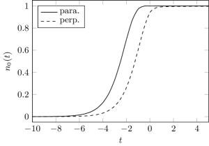
Figure 2: Time evolution of the occupation of the molecular ground state level $n_{0}$ in front of an Al₂O₃ surface for parallel (solid line) and perpendicular (dashed line) molecule orientation. The molecule’s kinetic energy was fixed to $50\,meV$. The curves were calculated from Eq. (29).

In the following we present numerical results for the two principal molecule orientations, that is, for the molecular axis aligned perpendicular ($\varphi=\frac{\pi}{2}$) and parallel ($\varphi=0$) to the surface.

First, we consider the capturing of a metal electron into the molecular ground state level, which was described in Sec. 2. Figure 2 shows the evolution of the ground state level’s occupation $n_{0}(t)$ as calculated from Eq. (29) for the case of an Al₂O₃ surface at a kinetic energy of $50\,meV$. We clearly see that the process is very efficient, since the molecular vacancy is completely filled within the incoming branch of the trajectory for both orientations.The efficiency is higher in parallel orientation. Complete filling of the ground state hole is achieved in that case at about $t=-1$, corresponding to a molecule-surface distance of approximately $4.92\,a_{B}$. In the perpendicular orientation, on the other hand, complete filling is only reached at about $t=0$ which corresponds to the molecule’s turning point $z_{0}=4.42\,a_{B}$.

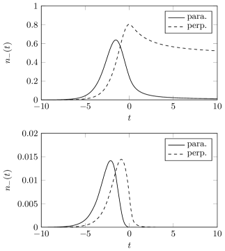
Figure 3: Fraction of negative ions versus time for the surface-induced decay process (upper panel) and the natural decay reaction (lower panel) in front of an Al₂O₃ surface at a molecular kinetic energy of $50\,meV$. The solid lines represent the parallel molecule orientation, whereas the dashed lines denote the perpendicular orientation. The results were calculated from Eq. (70b).

Next, we focus on the decay of a negative ion generated by electron capture. To estimate the relative strength of the surface-induced and the natural decay channel, respectively, we treat them separately. Figure 3 shows the time evolution of the fraction of negative ions as calculated from Eq. (70b) for both processes in front of an Al₂O₃ surface at $\varepsilon_{\text{kin}}=50\,meV$. As we see, within the incoming branch the portion of negative ions first increases due to the efficiency of the electron capture into the ground state and the finiteness of the decay rates. At some point within the incoming branch, however, the decay process starts to outbalance the generating reaction, resulting in a decrease of the negative ion fraction. Since the surface-induced decay process is driven by the molecule-surface interaction (41), which vanishes at large distances from the solid, the negative ion share saturates to a finite value in this case (see upper panel of Fig. 3). For the parallel orientation the saturation level is much lower than for the perpendicular orientation. This is caused by the antisymmetry of the molecular wave functions in the plane normal to the molecule’s axis. In the parallel orientation this antisymmetry is broken by the surface, which results in a significantly enlarged matrix element, and hence in a higher rate of decay. For the natural decay, on the other hand, the decay rate is constant, and thus the negative ion fraction eventually drops to zero (see lower panel of Fig. 3).

An important point to notice is that the portion of negative ions is about two orders of magnitude higher in the surface-induced decay as compared to the natural decay. The natural decay rate must thus be considerably larger than the surface-induced decay rate. Hence, the latter can be neglected in the present situation. It could, however, become important for material combinations that allow for projectile turning points closer to the surface. This would lead to an increase in the matrix element, which in turn results in a higher decay rate.

To calculate the fractions of metastables $n_{*}$ and ground state molecules $n_{g}$ from Eqs. (70a) and (70c), respectively, we focus therefore, in view of the above discussion, exclusively on the natural decay and neglect the surface-induced decay channel. The results are depicted in Fig. 4. Note that with the decrease of the fraction of metastables the ground state share almost immediately rises by the same amount, which is due to the rather large decay rate for natural decay. The fractions $n_{*}$ and $n_{g}$ can be related to the occupancies of the molecular levels $n_{0}$ and $n_{1}$ by means of Eq. (71).

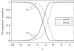
Figure 4: Time evolution of the fractions of metastables $n_{*}$ and ground state molecules $n_{g}$ in parallel (solid lines) and perpendicular (dashed lines) orientation for an Al₂O₃ surface at a molecular kinetic energy of $50\,meV$. Only the natural decay channel was considered. The curves were obtained by employing Eqs. (70a) and (70c), respectively.

We now turn to the spectrum of emitted electrons, which can be calculated from Eq. (73). Figure 5 shows the electronic spectrum at $t=\infty$, again for the case of Al₂O₃ and $\varepsilon_{\text{kin}}=50\,meV$, while neglecting the surface-induced decay channel. In both molecular orientations the spectrum exhibits a strong cut-off for energies below approximately $1\,eV$. This is a direct consequence of the image potential, trapping low energy electrons close to the surface, which was incorporated into our calculation by means of the quantity $\alpha(\varepsilon_{q_{z}},t)$ (see Eq. (43)). Following the low energy cut-off, the spectra show a strong peak at about $1.8-1.9\,eV$, before they slowly fall off towards zero for larger energies. Examining the curves we further note that the spectrum is larger in the parallel orientation than in the perpendicular orientation. This can again be attributed to the trapping effect. From Fig. 3 we know that in perpendicular geometry the negative ion is generated and destroyed closer to the surface than in parallel orientation. The image potential and hence the trapping effect are thus particularly strong in that case which in turn reduces the efficiency of electron emission.

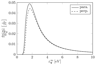
Figure 5: Spectrum of emitted electrons for an Al₂O₃ surface in parallel (solid lines) and perpendicular (dashed lines) orientation at $t=\infty$, as calculated from Eq. (73). The molecule’s kinetic energy was fixed to $50\,meV$. Only the natural decay process was taken into account.

Finally, we calculate the secondary electron emission coefficient $\gamma_{e}$, which is the area beneath curves of the type shown in Fig. 5. We specifically consider Al₂O₃, MgO, SiO₂, and diamond. The electronic parameters for these substances are listed in Table 1. We assume the turning point formula given in Marbach2011Auger to be valid for all of these materials. Hence, we can neglect the surface-induced decay process.

Figure 6 depicts the variation of the secondary electron emission coefficient $\gamma_{e}$ with the molecule’s kinetic energy $\varepsilon_{kin}$ for the aforementioned materials as calculated from Eq. (73). Leaving MgO aside (for a discussion see below), the $\gamma_{e}$-coefficients are on the order of $10^{-1}$ over the whole range of kinetic energies. The rather large values for $\gamma_{e}$ can be attributed to the shape resonance $\mathrm{N_{2}^{-}}(^{2}\Pi_{g})$ which is not only efficiently formed in front of the surface but also quickly decays thereby releasing an electron. Atomic projectiles, for instance, metastable argon, which cannot form a metastable negative ion, will lead to much smaller $\gamma_{e}$ values.

The secondary electron emission coefficient we find for metastable nitrogen hitting a dielectric surface agrees rather well with the $\gamma_{e}$-coefficient which is required for a convergent, self-consistent kinetic simulation of DBDs taking this particular surface collision process into account Brandenburg2005Diffuse . In keeping with our initial motivation, the effective microscopic model is thus indeed capable to provide input data with sufficient accuracy for the kinetic modelling of gas discharges.

Let us now analyze Fig. 6 in more detail. The $\gamma_{e}$-coefficients increase with decreasing kinetic energy. This can be explained by the enlarged molecule-surface interaction time and the narrowed turning point which lead to a more effective filling of the ground state hole at lower projectile velocities. Apart from this obvious monotony property, the specific form of the particular graphs is, however, not easily understood. The reason for this is the complex dependence of the secondary electron emission coefficient on the surface’s band structure and its static dielectric constant. For the materials we considered a few general remarks, however, can be given.

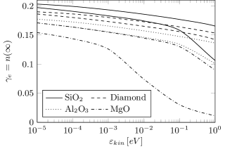
Figure 6: Secondary electron emission coefficient $\gamma_{e}$ for several different dielectric surfaces plotted against the molecule’s kinetic energy $\varepsilon_{kin}$. For each material two curves are depicted. The upper corresponds to the parallel molecule orientation, whereas the lower identifies the perpendicular molecule orientation. All results were obtained from Eq. (73).

First, we note that the emission coefficient is sensitive to the efficiency of the electron capture into the molecular hole level. A high efficiency results in negative ions getting produced at large distances from the surface. The subsequent electron emission will thus also take place at large distances, because of the large natural decay rate of the ions. This is beneficial to the emission coefficient, as the image potential trapping is less severe at larger distances. The efficiency of the electron capture in turn is determined by the alignment of the solid’s valence band to the molecular hole level. Since the filling of the molecular vacancy is a resonant tunneling process, the vacancy level $\varepsilon_{0}$ has to be degenerate to occupied states within the surface in order to allow for an efficient generation of negative ions. In addition, the electron capture is more productive if the degeneracy appears at higher energies within the valence band. This is due to the fact that at higher energies the wave functions of the electrons within the solid have a larger extension outside the solid. Thus their overlap with the molecular wave function is increased, which directly influences the matrix element and thus the efficiency of the electron capture. For MgO both conditions, degeneracy and higher energies within the valence band, are violated since the molecular hole level $\varepsilon_{0}$ shifts downwards out of the valence band at small distances (see Fig. 1). As a result MgO has the smallest emission coefficient of the materials under consideration.

Secondly, a higher dielectric constant seems to have an adverse effect on the value of $\gamma_{e}$, since for the most part the emission coefficients for SiO₂ and diamond, both having lower dielectric constants, are higher than the emission coefficient of Al₂O₃  which possesses a higher dielectric constant (see Table 1). This effect can probably be attributed to the amount of image potential trapping of slow electrons, which is proportional to $(\varepsilon_{r}^{b}-1)/(\varepsilon_{r}^{b}+1)$ (see Eqs. (6) and (43)). This factor increases with $\varepsilon_{r}^{b}$. Thus, the image potential and with it the effect of trapping is enlarged for higher dielectric constants.

5 Conclusion

In this work we described a generic effective microscopic model for secondary electron emission due to collision of metastable molecules with dielectric surfaces. As an illustration we applied the model to $\mathrm{N_{2}}(^{3}\Sigma_{u}^{+})$ hitting a dielectric surface, focusing on the RCT channel (2) which is particularly strong because this molecule forms a shape resonance upon electron capture. In addition, the competing Auger process (1) is energetically blocked for the dielectrics commonly used in gas discharge physics and needs thus not to be considered.

Our model depends only on a small number of material parameters. As far as the surface is concerned, these parameters include the electron affinity $\varepsilon_{\alpha}$ of the solid, its band gap $\varepsilon_{g}$, and the width of its valence band $\Delta\varepsilon_{V}$ as well as its static dielectric constant $\varepsilon_{r}^{b}$. Any surface that can be parameterized by such a set can in general be treated within our model. With a few modifications the model can also be applied to metallic surfaces and other molecular and atomic projectiles.

We presented numerical results for Al₂O₃, MgO, SiO₂, and diamond surfaces. The electronic parameters of the surface in question are crucial for the overall efficiency of the RCT process. The generation of the shape resonance $\mathrm{N_{2}^{-}}(^{2}\Pi_{g})$ upon electron capture into the lower ionization level of $\mathrm{N_{2}^{-}}(^{2}\Pi_{g})$ is efficient only when the molecular level stays well inside the valence band. Concerning the decay of the temporary negative ion we found the surface-induced process to be about two orders of magnitude weaker than the auto-decay. The surface-induced decay channel can thus be neglected for the situations we investigated. We found the spectrum of the emitted electron to be strongly peaked at about $1.8-1.9\,eV$. In a gas discharge, however, the auto-decay occurs close to the plasma wall where the sheath potential is large. The emitted electron will thus immediately gain a kinetic energy which is substantially larger than the energy resulting from auto-decay.

Calculations of the secondary electron emission coefficient $\gamma_{e}$ for different surface materials finally yielded $\gamma_{e}$-values from $0.02$ to $0.2$ for collision energies ranging from $0.1\,\mu eV$ to $1\,eV$. Particularly for thermal energies the $\gamma_{e}$-values we obtain are of the order of $10^{-1}$ and thus coincide with the values deduced from kinetic simulations of dielectric barrier discharges which take this particular secondary electron emission process into account. Hence, despite its simplicity effective microscopic modelling can capture the essential physics of secondary electron emission from surfaces due to impacting metastable molecules and is thus capable to fill some of the gaps in the molecule-surface collisions’ reference data which are required for the kinetic modeling of gas discharges.

References

• (1) F. Massines, N. Gherardi, N. Naudé, P. Ségur, The European Physical Journal Applied Physics 47(2), 22805 (2008)
• (2) Y.B. Golubovskii, V.A. Maiorov, J. Behnke, J.F. Behnke, Journal of Physics D: Applied Physics 35(8), 751 (2002)
• (3) R. Brandenburg, V.A. Maiorov, Y.B. Golubovskii, H.E. Wagner, J. Behnke, J.F. Behnke, Journal of Physics D: Applied Physics 38(13), 2187 (2005)
• (4) C. Punset, J.P. Boeuf, L.C. Pitchford, Journal of Applied Physics 83(4), 1884 (1998)
• (5) G. Auday, Ph, J. Galy, Journal of Applied Physics 88(8), 4871 (2000)
• (6) T.J. Vink, A.R. Balkenende, R.G.F.A. Verbeek, H.A.M. van Hal, S.T. de Zwart, Applied Physics Letters 80(12), 2216 (2002)
• (7) Y.P. Raizer, Gas discharge physics (Springer-Verlag, Berlin, 1991)
• (8) J. Marbach, F.X. Bronold, H. Fehske, Physical Review B 84, 085443 (2011)
• (9) N. Lorente, D. Teillet-Billy, J.P. Gauyacq, Surface Science 432(1-2), 155 (1999)
• (10) P. Stracke, F. Wiegershaus, S. Krischok, V. Kempter, Surface Science 396(1-3), 212 (1998)
• (11) Y.C. Yeo, T.J. King, C. Hu, Journal of Applied Physics 92(12), 7266 (2002)
• (12) S. Ciraci, I.P. Batra, Physical Review B 28(2), 982 (1983)
• (13) J. Robertson, Reports on Progress in Physics 69(2), 327 (2006)
• (14) M.J. Rutter, J. Robertson, Computational Materials Science 10(1-4), 330 (1998)
• (15) J. Robertson, K. Xiong, S.J. Clark, phys. stat. sol. (b) 243(9), 2054 (2006)
• (16) S. Bhagavantam, D.A.A.S.N. Rao, Nature 161, 729 (1948)
• (17) Y.S. Kim, S.H. Yoon, S.G. Ahn, C.R. Hong, H. Yang, Electronic Materials Letters 4(3), 113 (2008)
• (18) M. Tobita, S. Ho, J. Chem. Theory Comput. 4(7), 1057 (2008)
• (19) J. Fontanella, C. Andeen, D. Schuele, Journal of Applied Physics 45(7), 2852 (1974)
• (20) E. Schreiber, H.J. Fitting, Journal of Electron Spectroscopy and Related Phenomena 124(1), 25 (2002)
• (21) S. Ciraci, S. Ellialtioǧlu, Physical Review B 25(6), 4019 (1982)
• (22) U. Kaldor, The Journal of Chemical Physics 81(5), 2406 (1984)
• (23) M. Honigmann, R.J. Buenker, H.P. Liebermann, The Journal of Chemical Physics 125(23), 234304 (2006)
• (24) D.M. Newns, K. Makoshi, R. Brako, J.N.M. van Wunnik, Physica Scripta 1983(T6), 5 (1983)
• (25) H.D. Hagstrum, Physical Review 96(2), 336 (1954)
• (26) J.W. Gadzuk, Surface Science 6(2), 133 (1967)
• (27) P. Kürpick, U. Thumm, Physical Review A 54(2), 1487 (1996)
• (28) A. Blandin, A. Nourtier, D.W. Hone, Journal de Physique 37(4), 369 (1976)
• (29) T. Mii, K. Makoshi, Surface Science 363(1-3), 145 (1996)
• (30) A. Dreuw, L.S. Cederbaum, International Journal of Mass Spectrometry 188(3), 199 (1999)