Abstract

An entanglement Rényi entropy for a spatial partition of a system is studied in conformal theories which admit a dual description in terms of an anti-de Sitter gravity. The divergent part of the Rényi entropy is computed in 4D conformal ${\cal N}=4$ super Yang-Mills theory at a weak coupling. This result is used to suggest a holographic formula which reproduces the Rényi entropy at least in the leading approximation. The holographic Rényi entropy is an invariant functional set on a codimension 2 minimal hypersurface in the bulk geometry. The bulk space does not depend on order $n$ of the Rényi entropy. The holographic Rényi entropy is a sum of local and non-local functionals multiplied by polynomials of $1/n$.

1 Introduction

A holographic description of many-body systems, including quantum field and condensed matter theories, in terms of gravity theories one dimension higher is an active research area. One of the aims here is to get new insights in situations where traditional methods meet difficulties, in regimes of strong couplings, for a example.

Quantum entanglement is one of those notions which carries an information about strength of correlations in a system. If a quantum system specified by a density matrix $\hat{\rho}$ is divided spatially onto parts, $A$ and $B$, one can define a reduced density matrix, say, for the region $A$,

$$\hat{{\rho}}_{A}=\mbox{Tr}_{B}\hat{\rho}~{}~{},$$ (1.1)

by taking trace over the states located in the region $B$. To quantify the degree of entanglement one introduces the entanglement entropy

$$S_{A}=-\mbox{Tr}_{A}\hat{{\rho}}_{A}\ln\hat{{\rho}}_{A}~{}~{},$$ (1.2)

and the entanglement Rényi entropy of order $n$

$$S^{(n)}_{A}={\ln\mbox{Tr}_{A}\hat{{\rho}}^{~{}n}_{A}\over 1-n}~{}~{},$$ (1.3)

where $n=2,3,...$. Formally $S_{A}=\lim_{n\to 1}S^{(n)}_{A}$.

In seminal papers [1, 2] Ryu and Takayanagi suggested a ”holographic formula” for calculation of entanglement entropy in conformal field theories (CFT) which admit a dual description in terms of anti-de Sitter (AdS) gravity. For a $d$ dimensional CFT spatially divided by a surface $\cal B$ the corresponding entropy of entanglement between the two parts is given by the Bekenstein-Hawking-like formula

$$S(\tilde{\cal B})={\mbox{vol}(\tilde{\cal B})\over 4G_{N}^{(d+1)}}~{}~{}~{}.$$ (1.4)

Here $G_{N}^{(d+1)}$ is a gravitational constant in a dual gravity theory and $\mbox{vol}(\tilde{\cal B})$ is the volume of a certain codimension 2 hypersurface $\tilde{\cal B}$ lying in the bulk. The definition of $\tilde{\cal B}$ is a classical Plateau problem: $\tilde{\cal B}$ has the least volume among the codimension 2 hypersurfaces in the bulk whose asymptotic infinity belongs to a conformal class of $\cal B$. There are extra, topological, requirements [3] for the choice of $\tilde{\cal B}$ to distinguish between cases when the entropy corresponds to the reduced matrix $\hat{{\rho}}_{A}$ or $\hat{{\rho}}_{B}$.

Formula (1.4) passes non-trivial tests. It reproduces known explicit expressions obtained by direct computations in 2D and 4D CFT’s. Among recent interesting applications of (1.4) are works on critical phenomena [4], higher dimensional extensions of the $c$-theorems [5]-[7], boundary effects in entanglement entropy [8] and many others, see [9] for a general review, and [10] for a possible role of entanglement in the origin of the entropy of black holes.

It is not much known about entanglement Rényi entropy (ERE) (1.3) in field theory models and about its holographic representation. An extensive analysis, mainly in 2D CFT’s, for two disjoint intervals was done in [11]. In [12] the logarithmic part of ERE was obtained for a massless scalar field in Minkowsky space-time and spherical entangling surface $\cal B$. The idea of [12] is that in the given example the reduced density matrix $\hat{{\rho}}_{A}$, see (1.1), can be converted in a thermal density matrix. This method was applied in [13] to get ERE for free scalar and spinor fields in 3 dimensions. The same idea was used in [14] to calculate ERE in various holographic models.

The definition of a holographic ERE may require a smooth modification of the bulk geometry with dependence of the bulk metric on order $n$. This possibility was explored in [14] by identifying ERE in an effective thermal state in the boundary CFT with an entropy of a black hole in the bulk. In our work we study another option by assuming that the bulk geometry in the definition of the holographic ERE does not depend on $n$. We calculate leading terms of the entanglement Rényi entropy (1.3) and use this information to suggest a corresponding generalization of the Ryu-Takayanagi formula.

Our computations done in the limit of the weak coupling are summarized by the formula

$$S^{(n)}({\cal B})\simeq\sum_{p=2}^{d-1}\Lambda^{d-p}{s^{(n)}_{~{}p}\over d-p}+s^{(n)}_{~{}d}\ln(\Lambda\mu)+...~{}~{},$$ (1.5)

where $d$ is the dimensionality of the space-time (a boundary theory), $\Lambda$ is an ultraviolet cutoff, $\mu$ is a typical scale of the theory. The canonical mass dimensions of $\Lambda$ and $\mu$ are $+1$ and $-1$, respectively. We assume that the space and, consequently, ${\cal B}$ have no boundaries. One can show then that $s^{(n)}_{~{}p}=0$ for odd $p$.

Our result for 4D CFT (${\cal N}=4$ $SU(N)$ supersymmetric Yang-Mills theory) is that $s^{(n)}_{~{}2}$ is proportional to $\gamma_{n}A({\cal B})$, where $A({\cal B})$ is the area of ${\cal B}$ and $\gamma_{n}=n^{-1}$. The coefficient $s^{(n)}_{~{}4}$ is related to the conformal anomaly. It is a scale invariant functional of the following structure:

$$s^{(n)}_{~{}4}=d(N)\left(a(\gamma_{n})F_{a}+c(\gamma_{n})F_{c}+b(\gamma_{n})F_{b}\right)~{}~{},$$ (1.6)

where $d(N)=N^{2}-1$, $F_{a}$ is related to the Euler characteristic of ${\cal B}$, $F_{c}$ is an integral of a projection of the Weyl tensor on ${\cal B}$, and $F_{b}$ is constructed solely of the extrinsic curvatures of ${\cal B}$. Coefficients $c(\gamma_{n})$ and $a(\gamma_{n})$ are 3d order polynomials of $\gamma_{n}$ which we compute by methods of the spectral geometry. Our method does not allow one to fix $b(\gamma_{n})$.

It is the structure of Eqs. (1.5), (1.6) which motivates our suggestion of a holographic ERE. The main result here is formula (3.22) which reproduces (1.5), (1.6). The holographic ERE coincides with Ryu-Takayanagi formula (1.4) at $n=1$ but it has a more complicated structure, in general. The holographic Rényi entropy (3.22) in $d=4$ is an invariant functional set on a codimension 2 minimal hypersurface $\tilde{\cal B}$ in the bulk which does not depend on $n$. Similar to (1.6) the entropy functional is linear combination of polynomials related to $a(\gamma_{n})$, $b(\gamma_{n})$, $c(\gamma_{n})$ and 4 different invariants. One of the invariants is $\mbox{vol}(\tilde{\cal B})$, two other are analogous to $F_{c}$ and $F_{b}$ and expressed with the help of curvatures in the bulk. The functional corresponding to $F_{a}$ is non-local logarithmic correction $\ln\mbox{vol}(\tilde{\cal B})$.

The work is organized as follows. Computations of the UV part of ERE in 2D and 4D CFT’s along with derivation of (1.5), (1.6) are presented in Sec. 2. The holographic entanglement Rényi entropy is suggested in Sec. 3. Sec. 4 contains a discussion of the results and concluding remarks. In particular, we speculate here on how the holographic formulas for ERE and for the entanglement entropy may appear in quantum gravity. The proposal of Sec. 3 is based on asymptotic behavior of different curvature invariants near the AdS boundary. Proofs of corresponding mathematical statements, some of which are new, are collected in Appendices. We show in Appendix B that the tilt angle of a minimal hypersurface $\tilde{\cal B}$ near a boundary of an asymptotically AdS space is determined by the extrinsic curvature of $\cal B$. This enables one to derive asymptotic embedding equations of $\tilde{\cal B}$ from pure geometrical considerations, see Appendix C.

2 Rényi entropy in conformal theories

2.1 Basic definitions

We consider a conformal field theory (CFT) set on a $(d-1)$-dimensional constant time hypersurface $\Sigma$. The spacetime is assumed to be static. The CFT density matrix $\hat{\rho}$ is chosen to be thermal, $\hat{\rho}=e^{-\hat{H}/T}/Z(T)$, where $T$ is the temperature, $\hat{H}$ is a Hamiltonian, and $Z(T)=\mbox{Tr}~{}\exp(-\hat{H}/T)$ is a partition function of the CFT.

It is convenient to introduce an ’entanglement partition function’ (EPF) associated to division of $\Sigma$ onto the parts $A$ and $B$ by a surface $\cal B$,

$$Z(n,T)=\mbox{Tr}_{A}\left(\mbox{Tr}_{B}~{}e^{-\hat{H}/T}\right)^{n}~{}~{},$$ (2.1)

where $n$ are natural numbers. At $n=1$ the two partition functions coincide, $Z(1,T)=Z(T)$. As follows from (1.1) and (2.1), the entanglement entropies can be expressed as

$$S(T)=-\lim_{n\rightarrow 1}~{}\left(n{\partial\over\partial n}-1\right)\ln Z(n,T)~{}~{}~{},$$ (2.2)

$$S^{(n)}(T)={1\over 1-n}\left(\ln Z(n,T)-n\ln Z(T)\right)~{}~{}.$$ (2.3)

In (2.2) one takes the limit $n\to 1$ by going from discrete to a continuous $n$. Arguments in support of this procedure can be found in [15]. We imply but omit in (2.1), (2.2), (2.3) the index $A$ (compare with (1.2), (1.3)). The ground state EPF, $Z(n)$, can be obtained from $Z(n,T)$ in the limit $T\to 0$.

In a quantum field theory the partition function $Z(T)$ is represented as a functional integral over field configurations which live on a Euclidean static $d$ dimensional manifold ${\cal M}$ with the constant time sections $\Sigma$. The orbits of the Killing vector field generating translations in Euclidean time are the circles $S^{1}$ with the length equal $1/T$.

Analogously, $Z(n,T)$ can be written in terms of a path integral where field configurations are set on a ’replicated’ manifold ${\cal M}_{n}$ which is glued from $n$ copies (replicas) of $\cal M$ along some cuts which meet on $\cal B$. An explicit construction of ${\cal M}_{n}$ is described in [16]. For our purpose it is enough to know that ${\cal M}_{n}$ are locally identical to $\cal M$ but have nontrivial topologies: ${\cal M}_{n}$ have conical singularities on $\cal B$ with the length of a small unit circle around each point on $\cal B$ equal $2\pi n$.

The partition function in a free CFT, therefore, is

$$-\ln Z(n)=\frac{1}{2}\sum_{i}\eta_{i}\ln\det(\mu^{2}\Delta^{(i)})~{}~{},$$ (2.4)

where $\Delta^{(i)}$ are Laplace operators for different fields which enter the model, $\eta_{i}=+1$ for Bosons and $\eta_{i}=-1$ for Fermions, $\mu$ is a scale parameter. The base manifold for the Laplace operators is ${\cal M}_{n}$. Determinant of an operator $L$ can be defined, for example, by the Ray-Singer formula: $\ln\det L=-\zeta^{\prime}(0;L)$ in terms of a first derivative of the zeta-function $\zeta(s;L)$ of $L$. For our purposes we use only scalar, spinor and vector Laplacians which are, respectively, $\Delta^{(0)}=-\nabla^{2}+\xi R$, $\Delta^{(1/2)}=(i\gamma^{\mu}\nabla_{\mu})^{2}$, $(\Delta^{(1)})^{\nu}_{\mu}=-\nabla^{2}\delta^{\nu}_{\mu}+R^{\nu}_{\mu}$. Here $R$, $R^{\nu}_{\mu}$ are the scalar curvature and the Ricci tensor. Quantization of vector fields is done in the Lorentz gauge and produces a couple of ghost fields. The Laplacians $\Delta^{(0)}$ for ghosts have minimal coupling, $\xi=0$.

When the Laplace operators do not have zero eigenvalue modes the ultraviolet part of (2.4) is

$$-\ln Z(n)\simeq\sum_{p=0}^{d-1}\Lambda^{d-p}~{}{A_{p}(n)\over p-d}-A_{d}(n)\ln(\Lambda\mu)~{}~{},$$ (2.5)

$$A_{p}(n)\equiv\sum_{i}\eta_{i}A_{p}(\Delta^{(i)})~{}~{},$$ (2.6)

where $A_{p}(\Delta^{(i)})$ are the heat coefficients that appear in short $t$ expansions for the corresponding heat kernel operators on ${\cal M}_{n}$,

$$\mbox{Tr}~{}e^{-t\Delta^{(i)}}\simeq\sum_{p}A_{p}(\Delta^{(i)})~{}t^{(p-d)/2}~{}~{}.$$ (2.7)

If there are no boundaries $A_{p}(\Delta^{(i)})=0$ for odd $p$. The heat coefficients have been computed earlier by different authors. We give corresponding references and describe the coefficients more carefully in sec. 2.3, see Eqs. (2.23), (2.26). Equation (1.5) follows from (2.3), (2.5) if one puts

$$s^{(n)}_{~{}p}={nA_{p}(1)-A_{p}(n)\over n-1}~{}~{}.$$ (2.8)

The Ray-Singer definition takes into account only non-zero eigenvalues of an operator. Therefore, when a Laplace operator $\Delta^{(i)}$ has a certain number $N_{\mbox{\tiny{zm}}}^{(i)}$ of zero modes one should use in (2.5) a combination $A_{d}(\Delta^{(i)})-N_{\mbox{\tiny{zm}}}^{(i)}$. This results in the following modification of (2.8) for the partial entropy:

$$s^{(n)}_{~{}p=d}={nA_{d}(1)-A_{d}(n)\over n-1}+s^{(n)}_{\mbox{\tiny{zm}}}~{}~{},$$ (2.9)

$$s^{(n)}_{\mbox{\tiny{zm}}}=-{nN_{\mbox{\tiny{zm}}}(1)-N_{\mbox{\tiny{zm}}}(n)\over n-1}~{}~{},$$ (2.10)

$$N_{\mbox{\tiny{zm}}}(n)=\sum_{i}\eta_{i}N_{\mbox{\tiny{zm}}}^{(i)}~{}~{}.$$ (2.11)

The simplest example is a Laplace operator on a compact 2D manifold $\cal M$. Such an operator on $\cal M$ and on the corresponding replicated spaces ${\cal M}_{n}$, which are compact as well, has a single normalizable zero mode. Hence $s^{(n)}_{~{}p=2}=-1$. In general, the number of zero modes (and so $s^{(n)}_{~{}p=d}$) may depend on the order $n$. In what follows we ignore effects of zero modes.

2.2 2D CFT

A simplest 2D CFT consists of some number of free spinor and minimally coupled scalar fields. The Rényi entropy is given by (1.5) for $d=2$. There is only a logarithmic term. From (2.8) one gets the known result [17]

$$s^{(n)}_{~{}2}={c\over 12}(1+\gamma_{n}){\cal A}({\cal B})~{}~{},$$ (2.12)

where $c$ is the total number of fields (the sum of central charges), ${\cal A}({\cal B})$ is the number of points of ${\cal B}$ (for example, $A({\cal B})=2$ if ${\cal B}$ is an interval).

2.3 4D CFT

${\cal N}=4$ $SU(N)$ supersymmetric Yang-Mills theory in $d=4$ consists of 6 multiplets of conformally coupled scalar fields (with $\xi=1/6$), 4 multiplets of Weyl spinors, and 1 multiplet of gluon fields. Each multiplet is in adjoint representation of the $SU(N)$ group. Computations in the case of the zero coupling with the help of (2.8) yield

$$s^{(n)}_{~{}2}={d(N)\over 4\pi}\gamma_{n}{\cal A}({\cal B})~{}~{},$$ (2.13)

$$s^{(n)}_{~{}4}=d(N)\left(a(\gamma_{n})F_{a}+c(\gamma_{n})F_{c}+b(\gamma_{n})F_{b}\right)~{}~{},$$ (2.14)

where $d(N)=N^{2}-1$,

$$F_{a}=-{1\over 2\pi}\int_{{\cal B}}\sqrt{\sigma}d^{2}x~{}R({\cal B})=-2\chi~{}~{},$$ (2.15)

and $\chi$ is the Euler characteristic of ${\cal B}$ (since ${\cal B}$ is closed and has topology of $S^{2}$, hence $\chi=2$), $a(\gamma_{n})$ and $c(\gamma_{n})$ are the following polynomials:

$$a(\gamma_{n})={1\over 96}\left(\gamma_{n}^{3}+\gamma_{n}^{2}+7\gamma_{n}+15\right)~{}~{},$$ (2.16)

$$c(\gamma_{n})={1\over 32}\left(\gamma_{n}^{3}+\gamma_{n}^{2}+3\gamma_{n}+3\right)~{}~{}.$$ (2.17)

The functional $F_{c}$ is determined in terms of a projection $C_{ijij}$ of the Weyl tensor $C_{\mu\nu\lambda\rho}$ at $\cal B$,

$$F_{c}={1\over 2\pi}\int_{{\cal B}}\sqrt{\sigma}d^{2}x~{}C_{ijij}~{}~{},$$ (2.18)

$$C_{ijij}=C_{\mu\nu\lambda\rho}n_{i}^{\mu}n_{j}^{\nu}n_{i}^{\lambda}n_{i}^{\rho}~{}~{}.$$ (2.19)

$n_{i}$, $i=1,2$, are two unit mutually orthogonal outward pointing normal vectors to ${\cal B}$. The Weyl tensor is

$$C_{\mu\nu\lambda\rho}=R_{\mu\nu\lambda\rho}+{1\over d-2}\left(g_{\mu\rho}R_{\nu\lambda}+g_{\nu\lambda}R_{\mu\rho}-g_{\mu\lambda}R_{\nu\rho}-g_{\nu\rho}R_{\mu\lambda}\right)$$

$$+{R\over(d-1)(d-2)}\left(g_{\mu\lambda}g_{\nu\rho}-g_{\mu\rho}g_{\nu\lambda}\right)~{}~{},$$ (2.20)

where $R$, $R_{\mu\nu}$, $R_{\mu\nu\lambda\rho}$ are, respectively, the scalar curvature, the Ricci tensor and the Riemann tensor of $\cal M$. Finally,

$$F_{b}={1\over 2\pi}\int_{{\cal B}}\sqrt{\sigma}d^{2}x~{}\left({1\over(d-2)}k_{i}^{2}-\mbox{Tr}(k_{i}^{2})\right)~{}~{},$$ (2.21)

where $(k_{i})_{\mu\nu}=h_{\mu}^{\lambda}h_{\nu}^{\rho}(n_{i})_{\mu;\nu}$ are extrinsic curvatures of $\cal B$, $k_{i}=g^{\mu\nu}(k_{i})_{\mu\nu}$, $\mbox{Tr}(k_{i}^{2})=(k_{i})_{\mu\nu}(k_{i})^{\mu\nu}$. Note that $d=4$ in (2.20), (2.21) for theories in 4 dimensions.

The functionals $F_{c}$, $F_{b}$ (and certainly $F_{a}$) are invariant under conformal transformations of the metric

$$\bar{g}_{\mu\nu}(x)=e^{-2\omega(x)}g_{\mu\nu}(x)~{}~{},~{}~{}\bar{n}_{i}^{\mu}=e^{\omega}n_{i}^{\mu}~{}~{}.$$ (2.22)

Conformal transformations are discussed in Appendix A. The conformal invariance is a consequence of the properties of the heat coefficients.

Coefficient functions $c(\gamma_{n})$, $a(\gamma_{n})$, $b(\gamma_{n})$ are related to the contribution of conical singularities to the heat coefficients of Laplace type operators on singular base manifolds. The coefficients have the following structure:

$$A_{p}(\Delta^{(i)})=nA_{p}(\Delta^{(i)})_{n=1}+\bar{A}_{p}(\Delta^{(i)})~{}~{}.$$ (2.23)

The term related to the presence of the conical singularities, $\bar{A}_{p}(\Delta^{(i)})$, is proportional to $(1-n)$ and can be written as

$$\bar{A}_{p}(\Delta^{(i)})=(1-n)\eta_{i}s^{(n)}_{~{}p,i}~{}~{}.$$ (2.24)

It follows from (2.24) that $s^{(n)}_{~{}p,i}$ is a contribution to the $p$-th term of the Rényi entropy from a particular field

$$s^{(n)}_{~{}p}=\sum_{i}s^{(n)}_{~{}p,i}~{}~{},$$ (2.25)

see (2.8). If the singular part of the heat coefficient is represented as

$$\bar{A}_{4}(\Delta)=\bar{a}(\gamma_{n})F_{a}+\bar{c}(\gamma_{n})F_{c}+\bar{b}(\gamma_{n})F_{b}$$ (2.26)

calculations in four dimensions yield for $\bar{a}(\gamma_{n})$ and $\bar{c}(\gamma_{n})$ the values which are summarized in Table 1. For a gauge boson the given result takes into account a contribution of ghosts. For the sake of clarity we also give the relation between coefficients defined in (2.16), (2.17) and coefficients from Table 1

$$a(\gamma_{n})={1\over 1-n}(6\bar{a}_{0}(\gamma_{n})-4\bar{a}_{1/2}(\gamma_{n})+\bar{a}_{1}(\gamma_{n}))~{}~{},$$ (2.27)

$$c(\gamma_{n})={1\over 1-n}(6\bar{c}_{0}(\gamma_{n})-4\bar{c}_{1/2}(\gamma_{n})+\bar{c}_{1}(\gamma_{n}))~{}~{},$$ (2.28)

where indexes $0,1/2$ and $1$ correspond to scalar, Weyl spinor and vector fields, respectively.

Computations of coefficient $A_{2}$ for spin 1/2 and 1 can be found in [18] and [19] (along with references to spin 0 results). Computations of $A_{4}$ can be found in different works: for spin 0 in [20], [21], [22], for spin 1/2 in [23], and for spin 1 in [24]. Let us emphasize that all computations imply that conical singularities are located on a surface with vanishing extrinsic curvatures. Some information on the effect of the curvatures can be obtained from requirement that $A_{4}$ in conformal theories in $d=4$ is scale invariant, see, e.g. [25] for discussion of this property. As was pointed out in [21], [22] $A_{4}$ can be fixed up to adding some conformally invariant functional of extrinsic curvatures. This functional, $F_{b}$, is introduced in (2.21). It is a quadratic combination of the curvatures because $A_{4}$ has zero canonical mass dimension in $d=4$.

The coefficient $\bar{b}(\gamma_{n})$ has not been derived so far by a direct computation. As we show later by using holographic arguments of [26], $\bar{b}(\gamma_{n}=1)=1/4$. This means that function $\bar{b}(\gamma_{n})$ may be non-trivial. It should be mentioned that, if $F_{b}=0$, formula (2.14) can be used with unknown $\bar{b}(\gamma_{n})$ even in cases of non-vanishing extrinsic curvatures. An example is a spherical entangling surface in a theory in Minkowsky space-time. One can easily find corresponding ERE for this model in $d=4$ by using (2.24), (2.26) and results of Table 1. Here $F_{a}=-4$, $F_{c}=F_{b}=0$ and one finds, in particular, that $s^{(n)}_{4}=-(\gamma_{n}+1)(\gamma_{n}^{2}+1)/360$ for scalars, $s^{(n)}_{4}=-(\gamma_{n}+1)(7\gamma_{n}^{2}+37)/1440$ for Weyl spinors. Computations of the logarithmic ERE $s^{(n)}_{4}$ in this model have been done in [12],[13] by transforming the reduced density matrix to a thermal form. The results of [12],[13] completely agree with the result above.

As for ERE for the spherical entangling surface in the weakly coupled supersymmetric Yang-Mills theory the same computation yields

$$S^{(n)}(R)\simeq d(N)\left[{\Lambda^{2}\over 8\pi n}{\cal A}-{1\over 48n^{3}}(15n^{3}+7n^{2}+n+1)\ln(\Lambda^{2}{\cal A})\right]~{}~{},$$ (2.29)

where ${\cal A}=4\pi R^{2}$ is the area of the surface and $R$ is its radius. To write (2.29) we used (1.5), where the infrared cutoff parameter $\mu$ was replaced with the radius $R$. This result disagrees with a holographic computation of the same entropy in [14] where ERE was identified with the entropy of a black hole in the AdS gravity. The difference is in the dependence on $n$ (in [14] this dependence is not the ratio of polynomials). We return to discussion of this point in sec. 4.

Table 1: Coefficient functions of singular parts of the heat coefficients

field $\bar{c}(\gamma)$ $\bar{a}(\gamma)$ $c$ $a$ real scalar ${\gamma^{4}-1\over 480\gamma}$ ${\gamma^{4}-1\over 1440\gamma}$ ${1\over 120}$ ${1\over 360}$ Weyl spinor $-{7\gamma^{4}+10\gamma^{2}-17\over 1920\gamma}$ $-{7\gamma^{4}+30\gamma^{2}-37\over 5760\gamma}$ ${1\over 40}$ ${11\over 720}$ gauge Boson ${\gamma^{4}+10\gamma^{2}-11\over 240\gamma}$ ${\gamma^{4}+30\gamma^{2}+60\gamma-91\over 720\gamma}$ ${1\over 10}$ ${31\over 180}$

There is a relation of the functions $\bar{a}(\gamma_{n})$, $\bar{c}(\gamma_{n})$ to the conformal anomaly. The trace of the renormalized stress-energy tensor of the each field has the form

$$\langle T^{\mu}_{\mu}\rangle=-a~{}E-c~{}I~{}~{},$$ (2.30)

$$E={1\over 16\pi^{2}}\left(R_{\mu\nu\lambda\rho}R^{\mu\nu\lambda\rho}-4R_{\mu\nu}R^{\mu\nu}+R^{2}\right)~{}~{},$$ (2.31)

$$I=-{1\over 16\pi^{2}}C_{\mu\nu\lambda\rho}C^{\mu\nu\lambda\rho}~{}~{}.$$ (2.32)

Constants $a$ and $c$ are given in Table 1 and one can check that

$$c=\eta\partial_{\gamma}\bar{c}(\gamma=1)~{}~{},~{}~{}a=\eta\partial_{\gamma}\bar{a}(\gamma=1)~{}~{}.$$ (2.33)

(As earlier, $\eta=+1$ for Bosons and $\eta=-1$ for Fermions.) On a regular manifold $A_{4}$ is composed of integrals of $E$ and $I$. Each of these integrals can be defined also on a singular manifold, if $|\gamma-1|$ is small and terms $O((\gamma-1)^{2})$ are neglected, see [27]. Equation (2.33) follows from a property established first in [28] for scalar Laplacians with minimal coupling: up to terms proportional to $(\gamma-1)$ the coefficient $A_{4}$ in the heat trace asymptotic of a Laplace operator on a manifold with conical singularities coincides with the corresponding heat coefficient on a regular manifold obtained by ’smoothing’ conical singularities.

Relation of scaling properties of the entanglement entropy to the trace anomaly is discussed in [29],[7].

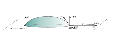
Figure 1: The figure shows the holographic surface $\tilde{\cal B}$ with normal vectors in a constant time section.

3 Toward a holographic description of the Rényi entropy

3.1 AdS gravity

The AdS/CFT conjecture [30]–[32] states that a supergravity theory in the anti-de Sitter (AdS) space is dual to a conformal field theory on the boundary of that region. Thus, we consider the $d+1$ dimensional gravity theory

$$I[g]=-{1\over 16\pi G_{N}^{(d+1)}}\int_{\tilde{\cal M}}d^{d+1}x\sqrt{g}\left(\tilde{R}+{d(d-1)\over l^{2}}\right)~{}~{}~{}$$ (3.1)

with the negative cosmological constant $-d(d-1)/(2l^{2})$. In what follows we put $l=1$, for simplicity.

Let $\tilde{\cal M}$ be a manifold with a metric $g_{KL}$ which is a solution to the Einstein equations in theory (3.1). Since $\tilde{\cal M}$ is asymptotically AdS $I[g]$ is not well defined. To avoid the volume divergencies of $I[g]$ one makes a cut of $\tilde{\cal M}$ at some $d$-dimensional hypersurface $\partial\tilde{\cal M}$. (We imply in (3.1) traditional boundary terms on $\partial\tilde{\cal M}$ but do not write them explicitly.) The cut of $\tilde{\cal M}$ is determined in suitably chosen coordinates by a fixed ’radius’ $\varrho$.

Let $\cal M$ be a $d$ dimensional manifold where a boundary CFT is defined on. The holographic relations require that metric induced on the boundary $\partial\tilde{\cal M}$ belongs to the conformal class of ${\cal M}$ in the limit of the infinite radius $\varrho$. The volume (infrared) divergences on the gravity side are identified with ultraviolet divergences in the CFT, that is $\varrho$ turns out to be related to a UV cutoff in the theory.

We denote scalar curvature, the Ricci tensor and the Riemann tensor of $\tilde{\cal M}$ by $\tilde{R}$, $\tilde{R}_{LP}$, $\tilde{R}_{LPKN}$, respectively.

3.2 Geometrical structures at AdS asymptotic

It is convenient to choose coordinates near $\partial\tilde{\cal M}$ in which the metric on $\tilde{\cal M}$ takes the form

$$ds^{2}=z^{-2}\left(dz^{2}+g_{\mu\nu}(z,x)dx^{\mu}dx^{\nu}\right)~{}~{}.$$ (3.2)

By definition, the embedding equation of $\partial\tilde{\cal M}$ is $z=const$. The relation with the radius is $\varrho=1/z$. If (3.2) is a solution to the bulk gravity equations the behavior of $g_{\mu\nu}(z,x)$ at small $z$ is known from the Fefferman-Graham asymptotic

$$g_{\mu\nu}(z,x)=g_{\mu\nu}(x)+z^{2}g_{\mu\nu}^{(1)}(x)+...~{}~{},$$ (3.3)

see e.g. [33], where

$$g_{\mu\nu}^{(1)}=-{1\over d-2}\left(R_{\mu\nu}-{g_{\mu\nu}R\over 2(d-1)}\right)~{}~{},$$ (3.4)

$g_{\mu\nu}(x)$ is a metric of $\cal M$, $R_{\mu\nu}$ and $R$ are curvatures of $\cal M$.

We assume that manifold $\cal M$ is static, so does the solution $\tilde{\cal M}$. The constant time section of $\tilde{\cal M}$ and its intersection with $\partial\tilde{\cal M}$ are denoted as $\tilde{\Sigma}$ and $\partial\tilde{\Sigma}$, respectively. Constant time section $\Sigma$ of $\cal M$ and $\partial\tilde{\Sigma}$ belong to the same conformal class.

We consider a minimal codimension 2 hypersurface $\tilde{\cal B}$ lying in a constant time section of $\tilde{\cal M}$. (The fact that the space is static implies that $\tilde{\cal B}$ is also minimal in $\tilde{\Sigma}$.) $\tilde{\cal B}$ ends on $\partial\tilde{\Sigma}$. It is required that the boundary $\partial\tilde{\cal B}$ of $\tilde{\cal B}$ is a surface conformal to the separating surface $\cal B$ in $\Sigma$.

Let $l,m$ be a pair of normal vectors to $\tilde{\cal B}$ such that $l^{2}=m^{2}=1$, $(l\cdot m)=0$. We choose direction of $l$ along a Killing field $\partial_{\tau}$ which generates time translations of the bulk manifold $\tilde{\cal M}$. (Let us emphasize that $\tau$ is a Euclidean time.) Once $l$ is chosen along $\partial_{\tau}$, $m$ is tangent to $\tilde{\Sigma}$. Position of $\tilde{\cal B}$ in $\tilde{\Sigma}$ is shown on Fig. 1. We also define 3 unit vectors $n,p,q$ at $\partial\tilde{\cal B}$ which are also tangent to $\tilde{\Sigma}$: $n$ is orthogonal to $\partial\tilde{\Sigma}$, $q$ is orthogonal to $\partial\tilde{\cal B}$ and tangent to $\tilde{\cal B}$, $p$ is orthogonal to $\partial\tilde{\cal B}$ and tangent to $\partial\tilde{\Sigma}$, see Fig. 1.

We need asymptotic relations for the metric on $\tilde{\cal B}$ similar to (3.2). Below we present a number of results, part of which are new. The details of computations can be found in Appendices B and C.

Since $\cal M$ is static $\cal B$ has a single non-trivial extrinsic curvature tensor in $\cal M$ which we denote $k_{\mu\nu}$. In general, $\tilde{\cal B}$ is tilted to $\partial\tilde{\Sigma}$. That is why there is a non-vanishing angle between vectors $m$ and $p$. If $\tilde{\cal B}$ is a minimal surface in asymptotically AdS space one finds (see Appendix B) the following asymptotic formula for the tilt angle:

$$\varphi\simeq{z\over d-2}~{}k~{}~{},$$ (3.5)

where $k$ is the trace of extrinsic curvature tensor $k_{\mu\nu}$ of $\cal B$. Surface $\tilde{\cal B}$ becomes orthogonal to $\partial\tilde{\Sigma}$ in the limit $z\to 0$.

The metric induced on $\tilde{\cal B}$ can be written in the form

$$ds^{2}(\tilde{\cal B})={1\over z^{2}}\left({dz^{2}\over\cos^{2}\varphi}+\sigma_{ab}(z,y)dy^{a}dy^{b}\right)~{}~{}.$$ (3.6)

Let $y^{a}$, $a=1,...d-2$, be coordinates on $\cal B$, and $\sigma_{ab}(y)=x^{\mu}_{~{},a}g_{\mu\nu}(x)x^{\nu}_{~{},b}$ be the metric induced on $\cal B$ under embedding $x^{\mu}=x^{\mu}(y)$. One finds the following asymptotic formula:

$$\sigma_{ab}(z,y)=\sigma_{ab}(y)-{z^{2}\over d-2}\left(kk_{ab}+R_{ab}-{\sigma_{ab}\over 2(d-1)}R\right)+..,$$ (3.7)

where $R_{ab}=x^{\mu}_{~{},a}x^{\nu}_{~{},b}R_{\mu\nu}$, $k_{ab}=x^{\mu}_{~{},a}x^{\nu}_{~{},b}k_{\mu\nu}$, see Appendix C.

In $d=4$

$$\mbox{vol}(\tilde{\cal B})=\int_{\cal B}\sqrt{\sigma}d^{2}y\left[{1\over 2\varepsilon^{2}}+\frac{1}{4}\ln{\mu\over\varepsilon}\left(-R({\cal B})+C_{ijij}+{k^{2}\over 2}-\mbox{Tr}(k^{2})\right)+...\right]$$

$$={1\over 2\varepsilon^{2}}A({\cal B})+{\pi\over 2}(F_{a}+F_{c}+F_{b})\ln{\mu\over\varepsilon}+...~{}~{},$$ (3.8)

where $\mu$ has a meaning of an infrared cutoff. This result coincides with computations of [29], see also [5].

Let us discuss invariant functionals on $\tilde{\cal B}$ which are integrals of curvature invariants. Since $\tilde{\cal M}$ is a solution to the bulk Einstein equations with the negative cosmological constant the scalar curvature and the Ricci tensor are known: $\tilde{R}=-(d+1)d$, $\tilde{R}_{LP}=-dg_{LP}$. These structures are fixed and are not related to geometrical characteristics of $\cal M$ and $\cal B$.

The other candidate is the Riemann tensor $\tilde{R}_{LPKN}$ of $\tilde{\cal M}$. In the asymptotic $\tilde{R}_{LPKN}\simeq-(g_{LK}g_{PN}-g_{LN}g_{PK})$ at $z\to 0$. One can also consider quantities connected with the geometry of $\tilde{\cal B}$. There are two such quantities: the scalar curvature $\tilde{R}_{B}$ and a quadratic combination of extrinsic curvature tensors of $\tilde{\cal B}$. Since $\tilde{\cal B}$ is static the single non-vanishing extrinsic curvature tensor $K_{LP}$ is defined for the normal vector $m$, see Fig. 1. $K_{LP}$ is traceless since $\tilde{\cal B}$ is minimal.

Thus, one has 3 possible invariants which behave at $z\to 0$ as follows:

$$\tilde{R}_{rsrs}(z,y)\equiv 2\tilde{R}_{LPKN}l^{L}m^{P}l^{K}m^{N}=-2+z^{2}C_{ijij}(y)+...~{}~{}~{},$$ (3.9)

$$\tilde{R}_{B}(z,y)=-(d-2)(d-1)+z^{2}\left(C_{ijij}(y)+{k^{2}\over d-2}-\mbox{Tr}(k^{2})\right)+...~{}~{}~{},$$ (3.10)

$$\mbox{Tr}K^{2}=K_{LP}K^{LP}=-z^{2}\left({k^{2}\over d-2}-\mbox{Tr}(k^{2})\right)+...~{}~{}~{},$$ (3.11)

see calculations in Appendix D. These asymptotics contain only conformally covariant structures: normal projection (2.19) of the Weyl tensor of $\cal M$ and combinations of extrinsic curvatures of $\cal B$, whose transformation properties are listed in Appendix A. The left hand sides of (3.9)-(3.11) are invariant with respect to bulk diffeomorphisms which have a subgroup of so called Penrose-Brown-Henneaux (PBH) transformations [34] which preserve the gauge (3.2). Since PBH transformations generate Weyl transformations of the metric on $\cal M$, only Weyl covariant structures appear on the right hand sides.

Note that invariants (3.9)-(3.11) are not actually independent:

$$\tilde{R}_{B}-\tilde{R}+2\tilde{R}_{ss}-\tilde{R}_{rsrs}-K^{2}+\mbox{Tr}(K^{2})=0~{}~{}.$$ (3.12)

Here $\tilde{R}_{ss}=(l^{L}l^{P}+m^{L}m^{P})\tilde{R}_{LP}$ and $K=0$ in the considered case. This identity is the known Gauss-Codazzi equation.

Formulas (3.8), (3.10) were obtained in [29] by using arguments based on properties of PBH transformations. We derive these and other relations straightforwardly in Appendix D.

3.3 Holographic entanglement entropy

It is instructive first to see how the geometrical structures above work to reproduce the entanglement entropy in 4D CFT. One uses the holographic formula (1.4), AdS/CFT dictionary which identifies the gravity coupling with the group parameter as $1/G_{N}^{(5)}=2N^{2}/\pi$ and finds the entanglement entropy in form (1.5) for the inverse order parameter $\gamma_{n}=1$. If the gravity cutoff is chosen as $\varepsilon=\Lambda^{-1}$ one gets relations

$$s_{2}^{(1)}={N^{2}\over 4\pi}~{}~{},~{}~{}s_{4}^{(1)}=N^{2}\left(\frac{1}{4}F_{a}+\frac{1}{4}F_{c}+\frac{1}{4}F_{b}\right)~{}~{}~{},$$ (3.13)

which coincide exactly with (2.13), (2.14), (2.16), (2.17) at large $N$. If the extrinsic curvature is non-zero one can use (3.13) to guess the coefficient at the invariant $F_{b}$ which has not been computed on the CFT side so far. One finds

$$b(\gamma_{n}=1)=1/4~{}~{}~{}.$$ (3.14)

This ‘holographic’ argument was first suggested in [26].

Formula (3.13) for $s_{4}^{(1)}$ does not reproduce a possible contribution of zero modes $s^{(n=1)}_{\mbox{\tiny{zm}}}$, see (2.9).

3.4 Holographic Rényi entropy

Our aim now is to find a holographic formula which would be able to reproduce Rényi entropy (1.5) with coefficients established in Sect. 2. To be more specific the holographic Rényi entropy $S(n,\tilde{\cal B})$ associated to an entangling surface $\cal B$ in the boundary CFT is considered to be a functional set on a codimension 2 minimal hypersurface $\tilde{\cal B}$ in $\tilde{\cal M}$. We conjecture that $S(n,\tilde{\cal B})$ is an invariant functional similar to (1.4) and is constructed from intrinsic and extrinsic geometrical structures of $\tilde{\cal B}$.

Let us emphasize that the bulk geometries $\tilde{\cal M}$, $\tilde{\cal B}$ are the same as in the Ryu-Takayanagi setup and they do not depend, therefore, on the order parameter $n$. It is the form of the functional which is allowed to contain $n$. This differs our approach from the recent conjecture of [14] where $n$ enters the metric of the bulk solutions.

The simplest case which illustrates our idea is the holographic formula for Rényi entropy of a 2D CFT. One can check that the following area functional:

$$S(n,\tilde{\cal B})\simeq{1\over 4G_{N}^{(3)}}{\gamma_{n}+1\over 2}\mbox{vol}(\tilde{\cal B})$$ (3.15)

reproduces (2.12) if we choose $c={3\over 2G_{N}^{(3)}}$.

To discuss 4D CFT we should consider several invariant structures associated to $\tilde{\cal B}$, first of all, $\mbox{vol}(\tilde{\cal B})$ and integrals over $\tilde{\cal B}$ of local invariants constructed from curvatures. Let us define the following functionals:

$$\tilde{F}_{c}={1\over 2\pi}\int_{\tilde{\cal B}}\sqrt{\tilde{\sigma}}d^{3}y\left[\tilde{R}_{rsrs}+2l^{-2}\right]~{}~{}~{},$$ (3.16)

$$\tilde{F}_{b}=-{1\over 2\pi}\int_{\tilde{\cal B}}\sqrt{\tilde{\sigma}}d^{3}y~{}\mbox{Tr}K^{2}~{}~{}~{},$$ (3.17)

where we denoted a metric induced on $\tilde{\cal B}$ by $\tilde{\sigma}$ and restored explicit dependence on the AdS radius $l$. These quantities are ’holographic duals’ of functionals $F_{c}$ and $F_{b}$, see (2.18), (2.21), in a sense that

$$\tilde{F}_{c}=F_{c}~{}l\ln{\mu\over\varepsilon}+...~{}~{}~{},$$ (3.18)

$$\tilde{F}_{b}=F_{b}~{}l\ln{\mu\over\varepsilon}+...~{}~{}~{}.$$ (3.19)

These results follow directly from (3.9) and (3.11). Integral of the scalar curvature $\tilde{R}_{B}$ according to (3.10) is reduced to a combination of $F_{c}$ and $F_{b}$. There is no need to consider this integral independently since it can be expressed in terms of (3.18) and (3.19) with the help of Gauss-Codazzi equality.

To find a holographic representation of the Rényi entropy in 4D CFT we also need an invariant functional ’dual’ to $F_{a}$, see (2.15). The problem is that $F_{a}$ is an integral of the scalar curvature of $\cal B$. This integral is a topological invariant only in $d=4$ when $\cal B$ has dimension 2. In other dimensions $F_{a}$ is neither topological nor Weyl invariant. On the other hand, the PBH transformations require that liner combinations of curvatures in AdS in any dimension correspond to Weyl invariant structures on the boundary, as in case of Eqs. (3.9)-(3.11). Therefore, the bulk functional corresponding to $F_{a}$ cannot be among local invariants linear in curvatures. The only local structure which produces $F_{a}$ is the volume $\mbox{vol}(\tilde{\cal B})$, see (3.8). However, the coefficient by $\mbox{vol}(\tilde{\cal B})$ is fixed by the leading (area) term in ERE.

By taking this into account one should look for non-local bulk functionals. For example, for ERE with entangling surface $\cal B$ having topology of $S^{2}$ ($F_{a}=-4$) one can choose

$$\tilde{F}_{a}=-2l\ln(\mbox{vol}(\tilde{\cal B})/l^{3})~{}~{}.$$ (3.20)

Equation (3.8) can be used to show that

$$\tilde{F}_{a}=F_{a}~{}l\ln{\mu\over\varepsilon}-2l\ln(A({\cal B})/\mu^{2})+...~{}~{}~{},$$ (3.21)

Certainly, (3.20) is not a single option and other non-local structures are possible. The choice of (3.20) seems to be the simplest. The logarithmic term in a holographic ERE is similar to logarithmic corrections to the Bekenstein-Hawking entropy, which are a rather common consequence of quantum effects, see e.g. [35]-[38].

Now one can check with the help of (3.8), (3.18), (3.19), and (3.21) that the following functional:

$$S(n,\tilde{\cal B})={1\over 4G_{N}^{(5)}}\left(\gamma_{n}\mbox{vol}(\tilde{\cal B})+2\pi l^{2}\left(\tilde{a}(\gamma_{n})\tilde{F}_{a}+\tilde{c}(\gamma_{n})\tilde{F}_{c}+\tilde{b}(\gamma_{n})\tilde{F}_{b}\right)\right)~{}~{},$$ (3.22)

$$\tilde{a}(\gamma_{n})=a(\gamma_{n})-\frac{1}{4}\gamma_{n}={1\over 96}(\gamma_{n}-1)\left(\gamma_{n}^{2}+2\gamma_{n}-15\right)~{}~{},$$ (3.23)

$$\tilde{c}(\gamma_{n})=c(\gamma_{n})-\frac{1}{4}\gamma_{n}={1\over 32}(\gamma_{n}-1)\left(\gamma_{n}^{2}+2\gamma_{n}-3\right)~{}~{},$$ (3.24)

$$\tilde{b}(\gamma_{n})=b(\gamma_{n})-\frac{1}{4}\gamma_{n}~{}~{},$$ (3.25)

reproduces (2.13), (2.14), (2.16), (2.17) at large $N$. Adding $-\frac{1}{4}\gamma_{n}$ in (3.23)-(3.25) compensates curvature terms ($F_{a}$,$F_{b}$, $F_{c}$) which come out from $\mbox{vol}(\tilde{\cal B})$, see (3.8).

Since $\tilde{a}(1)=\tilde{c}(1)=\tilde{b}(1)=0$ expression (3.22) coincides with Ryu-Takayanagi formula (1.4) in the limit $n\to 1$. It is also important to note that $S^{(n)}({\cal B})$, like (1.4), depends only on low-energy constants $G_{N}^{(5)}$ and $l$ which enter gravity action (3.1).

4 Discussion

We suggest (3.22) as a holographic formula for the entanglement Rényi entropy. One should emphasize that $S(n,\tilde{\cal B})$ reproduces at least the divergent part (1.5) of ERE in the conformal theory in four dimensions. Thus, additional terms may be needed in $S(n,\tilde{\cal B})$ to go beyond the given approximation.

One may note some differences between (3.22) and Ryu-Takayanagi expression (1.4). Unlike (1.4), the form of $S(n,\tilde{\cal B})$ explicitly depends on the dimension $d$. This can be seen by comparing (3.22) with a possible formula of holographic ERE for 2D CFT, see (3.15). In (3.15) the leading term remains finite in the limit $n\to\infty$ while in (3.22) the volume term vanishes.

Another distinction between (1.4) and (3.22) is that the minimal hypersurface $\tilde{\cal B}$ is not an exact extremal hypersurface for functional (3.22). (An extremal value of (3.22) is defined by varying position of the hypersurface under fixed background metric and $n$.) Note that $\tilde{\cal B}$ would be an extremal hypersurface if $\tilde{F}_{a}$ term alone were present. This term depends only on the volume $\mbox{vol}(\tilde{\cal B})$. However $S(n,\tilde{\cal B})$ includes also terms with $\tilde{F}_{b}$ and $\tilde{F}_{c}$ which depend on curvatures. Let us emphasize that the choice of $\tilde{\cal B}$ as an argument in the holographic ERE functional was crucial for finding the correspondence between bulk and boundary quantities.

What happens if $\tilde{\cal B}$ is replaced by a genuine extremal surface? Let us define (3.22) on a set of codimension 2 hypersurfaces $\tilde{\cal Q}$ in $\tilde{\cal M}$ specified by the same boundary condition as $\tilde{\cal B}$, that is $\partial\tilde{\cal Q}\sim{\cal B}$. Such hypersurfaces have infinitely large volume in the limit $z\to 0$. We also require that for $\tilde{\cal Q}$ the following restrictions are satisfied at $z\to 0$: $\mbox{Tr}~{}K^{2}\ll l^{-2}$ and $|\tilde{R}_{rsrs}+2l^{-2}|\ll l^{-2}$. These restrictions allow $\tilde{\cal B}$ to belong to the given set. They also guarantee that terms with $\tilde{F}_{b}$ and $\tilde{F}_{c}$ in functional $S(n,\tilde{\cal Q})$ are small compared to the volume term. To see this one should take into account that main contributions to integrals are picked up in a neighborhood of $z=0$.

Suppose that $S(n,\tilde{\cal Q})$ has an extremum on some hypersurface $\tilde{\cal Q}$ from the considered set. Extremal hypersurfaces may depend on $n$, in general. Since terms with $\tilde{F}_{b}$ and $\tilde{F}_{c}$ are small one can represent $\tilde{\cal Q}$ as $\tilde{\cal B}$ with a small perturbation, $\tilde{\cal Q}=\tilde{\cal B}+\tilde{\cal Q}_{1}$. Up to terms which are of the second order in the perturbation, $S(n,\tilde{\cal Q})\simeq S(n,\tilde{\cal B})$. The second order terms are given by some (non-local) functional on $\tilde{\cal B}$ quadratic in curvatures which enter $\tilde{F}_{b}$ and $\tilde{F}_{c}$. It is important that the second order terms are small compared to $S(n,\tilde{\cal B})$. Therefore, once $S(n,\tilde{\cal B})$ is used to reproduce ERE only in the logarithmic approximation it is safe to replace it with the extremal value $S(n,\tilde{\cal Q})$.

The entanglement Rényi entropy $S^{(n)}({\cal B})$ can be defined by formula (2.3) in terms of an entanglement partition function $Z(n)$. It is interesting to discuss if there is a holographic representation for $Z(n)$ which results in functional $S(n,\tilde{\cal B})$. We use a line of reasonings suggested in [3] to show that such a representation may be possible.

In a quantum field theory $Z(n)$ can be written in terms of a path integral where field configurations are located on a manifold ${\cal M}_{n}$ glued from $n$ copies of the physical manifold $\cal M$ along some cuts $\Sigma_{A}$ which meet on $\cal B$, see [16]. ($\cal B$ divides a constant time hypersurface in $\cal M$ on parts $\Sigma_{A}$ and $\Sigma_{B}$, the trace in the reduced density matrix (1.1) is taken over states on $\Sigma_{B}$.) The AdS/CFT correspondence implies that $Z(n)$ can be replaced by a partition function, $Z^{AdS}[{\cal M}_{n}]$, in AdS-gravity for which a given CFT is a ’boundary’ theory. The idea of [3] is that in a low-energy approximation one should look for a path integral representation of $Z^{AdS}[{\cal M}_{n}]$ with the condition that the conformal boundary of ”histories”, $\tilde{\cal M}_{n}$, involved in the path integral belongs to the conformal class of ${\cal M}_{n}$,

$$Z^{AdS}[{\cal M}_{n}]=\int_{\tilde{\cal M}_{n}:~{}\partial\tilde{\cal M}_{n}\sim{\cal M}_{n}}[Dg]\exp(-W[g])~{}~{}~{}.$$ (4.1)

Functional $W[g]$ is an effective action which is induced by quantum gravity or string theory dynamics in the AdS bulk. For regular boundary conditions $W[g]$ is approximated by classical action (3.1). Since the boundary manifolds have conical singularities application of (3.1) in this case is not obvious.

Although quantum gravity arguments are absent we make a suggestion for $W[g]$ consistent with the holographic ERE. For the given boundary conditions there are two types of geometries $\tilde{\cal M}_{n}$ which may contribute to (4.1) in a semiclassical approximation. One type includes spaces which are regular in the bulk, another type includes manifolds with conical singularities. We consider only singular geometries. They can be constructed for the given boundary conditions in the following way [3]. One starts from bulk geometries $\tilde{\cal M}$ such that $\partial\tilde{\cal M}\sim{\cal M}$. Then, one makes different cuts of $\tilde{\cal M}$ along $d$–dimensional hypersurfaces $\tilde{\Sigma}_{A}$ with the boundary condition $\partial\tilde{\Sigma}_{A}\sim\Sigma_{A}$, where $\Sigma_{A}$ is the corresponding cut in ${\cal M}$. The boundary condition does not fix $\tilde{\Sigma}_{A}$ uniquely. By taking $n$ identical copies of $\tilde{\cal M}$ with the same cut $\tilde{\Sigma}_{A}$ and gluing them along the cuts one gets a space $\tilde{\cal M}_{n}$ with the required boundary condition $\partial\tilde{\cal M}_{n}\sim{\cal M}_{n}$. The bulk spaces have conical singularities on codimension 2 hypersurfaces $\tilde{\cal Q}$ related to the entangling surface, $\partial\tilde{\cal Q}\sim\cal B$. The holographic ERE defined by AdS partition function and approximated by using (4.1) is

$$S^{AdS}(n)={1\over 1-n}\left(\ln Z^{AdS}[{\cal M}_{n}]-n\ln Z^{AdS}[{\cal M}]\right)\simeq{1\over n-1}\left(W(n)-nW(1)\right)$$ (4.2)

where $W(n)$ is a least value of the effective action on some singular space $\tilde{\cal M}_{n}$.

We want to find $W(n)$ by requiring that $S^{AdS}(n)\simeq S(n,{\cal B})$. It is natural to assume that the leading part of $W(n)$ is local and is similar to a divergent part of a QFT effective action on manifolds with conical singularities. The structure of the heat kernel coefficients (2.23) then implies that $W(n)$ is a sum of two terms: one is defined on a regular domain $\tilde{\cal M}_{n}/\tilde{\cal Q}$, the other is located on $\tilde{\cal Q}$ and induced by quantum effects on conical singularities. The term on a regular domain coincides with classical action (3.1). It is proportional to $n$ and does not contribute to ERE (4.2). The only possible form of the leading part of $W(n)$ which allows one to equate the two entropies, $S^{AdS}(n)\simeq S(n,\tilde{\cal Q})$, is

$$W(n)\simeq I[\tilde{\cal M}_{n}/\tilde{\cal Q}]+(n-1)S(n,\tilde{\cal Q})~{}~{}.$$ (4.3)

What is a singular manifold where the effective action has a least value? The fact that a saddle ’point’ is a singular manifold even without a matter source which supports the conical singularities should not be considered as a controversy. The extremum of $W(n)$ is defined within a restricted set of geometries. For other class of geometries which contribute to (4.1) and are regular in the bulk one should use another action. One should also note that (4.3) does not coincide with a classical action (3.1) naively taken on $\tilde{\cal M}_{n}$. In this case one would not get in (4.3) $\tilde{F}_{a}$, $\tilde{F}_{b}$ and $\tilde{F}_{c}$ terms. The two actions agree only in the limit $n\to 1$ up to terms linear in $(n-1)$.

Variations of the two terms in (4.3) are required to vanish independently. Variations of $I[\tilde{\cal M}_{n}/\tilde{\cal Q}]$ are subject to certain boundary conditions near conical singularities to preserve their structure. They result in the standard bulk gravity equations for (3.1). That is, locally $\tilde{\cal M}_{n}$ is one of solutions of AdS gravity. Minimization of $S(n,\tilde{\cal Q})$ implies that $\tilde{\cal Q}$ is an extremal hypersurface, thus, in the leading approximation we recover the holographic entanglement entropy $S(n,\tilde{\cal B})$ from $S^{AdS}(n)$.

Although the above ’derivation’ of holographic ERE is based on a number of assumptions it may be a plausible scenario. An explanation of Ryu-Takayanagi formula (1.4) seems to be its particular case which follows in the limit $n\to 1$. This gives a further support to earlier arguments presented in [3] and allows one to avoid their criticism in [11].

It would be very interesting to understand the behaviour of ERE in a strong coupling regime. Our approach to the holographic description of ERE should hold in this case but functions $\tilde{a}(\gamma_{n})$, $\tilde{b}(\gamma_{n})$, $\tilde{c}(\gamma_{n})$ in (3.22) may be different. The reason is that the logarithmic terms in the Renyi entropy for $n>1$ are not determined solely by the conformal anomaly. They are not protected from both perturbative and non-perturbative corrections, as was pointed out in [13]. This may be the reason why results of [14] for a spherical entangling surface disagree with weak coupling formula (2.29).

Our proposal may be compatible with the approach of [14] (after a proper redefinition of $\tilde{a}(\gamma_{n})$, $\tilde{b}(\gamma_{n})$, and $\tilde{c}(\gamma_{n})$) but to resolve the issue one needs to know quantum corrections to ERE.

Appendix A Conformal transformations

Several useful relations for conformal transformations of the metric of a $D$ dimensional manifold

$$\bar{g}_{\mu\nu}(x)=e^{-2\omega(x)}g_{\mu\nu}(x)~{}~{}$$ (A.1)

are listed below for the sake of completeness. Dimensionality $D$ in cases considered in our work is either $d+1$ or $d$, where $d$ is the dimensionality of the boundary CFT. One can find the following transformations:

$$\bar{R}_{\lambda\mu\nu\rho}=e^{-2\omega}\left[R_{\lambda\mu\nu\rho}+\omega_{\lambda\nu}g_{\mu\rho}-\omega_{\lambda\rho}g_{\mu\nu}-\omega_{\mu\nu}g_{\lambda\rho}-\omega_{\mu\rho}g_{\lambda\nu}+\right.$$

$$\left.\omega_{\mu}\omega_{\rho}g_{\lambda\nu}-\omega_{\nu}\omega_{\mu}g_{\lambda\rho}+\omega_{\nu}\omega_{\lambda}g_{\rho\mu}-\omega_{\lambda}\omega_{\rho}g_{\mu\nu}+\omega^{\alpha}\omega_{\alpha}(g_{\mu\nu}g_{\lambda\rho}-g_{\mu\rho}g_{\lambda\nu})\right]~{}~{},$$ (A.2)

$$\bar{R}_{\mu\nu}=R_{\mu\nu}+(D-2)\omega_{\mu\nu}+g_{\mu\nu}\Delta\omega+(D-2)\omega_{\mu}\omega_{\nu}+(2-D)\omega^{\alpha}\omega_{\alpha}~{}g_{\mu\nu}~{}~{},$$ (A.3)

$$\bar{R}=e^{2\omega}\left[R+2(D-1)\Delta\omega-(D-2)(D-1)\omega^{\alpha}\omega_{\alpha}\right]~{}~{},$$ (A.4)

where $\omega_{\mu}=\omega_{,\mu}$, $\omega_{\mu\nu}=\omega_{;\mu\nu}$. If there is a codimension 2 hypersurface with two normal vectors $n_{i}$ one can also establish the following scaling properties:

$$\bar{n}_{i}^{\mu}=e^{\omega}n_{i}^{\mu}~{}~{},$$ (A.5)

$$(\bar{k_{i}})_{\mu\nu}=e^{-\omega}\left[(k_{i})_{\mu\nu}-h_{\mu\nu}n_{i}^{\lambda}\omega_{,\lambda}\right]~{}~{},$$ (A.6)

$$\bar{C}_{ijij}=e^{2\omega}C_{ijij}~{}~{},$$ (A.7)

$$\bar{k}_{i}^{2}-(D-2)\mbox{Tr}(\bar{k}_{i}^{2})=e^{2\omega}\left(k_{i}^{2}-(D-2)\mbox{Tr}(k_{i}^{2})\right)~{}~{},$$ (A.8)

where $h_{\mu\nu}=g_{\mu\nu}-(n_{i})_{\mu}(n_{i})_{\nu}$ is the metric on the hypersurface, $(k_{i})_{\mu\nu}=h_{\mu}^{\lambda}h_{\nu}^{\rho}(n_{i})_{\mu;\nu}$ are its extrinsic curvatures, $C_{ijij}$ is the normal projection (2.19) of the Weyl tensor (2.20). Our convention is that $n_{i}$ are outward pointing vectors.

Appendix B Tilt angle of the holographic surface in AdS

To prove (3.5) for the tilt angle $\varphi$ shown on Fig. 1 we consider embedding of $\tilde{\cal B}$ described by the equation

$$z=\psi(x)~{}~{}~{}.$$ (B.1)

From definition of vectors $m$ and $n$ one finds

$$\sin\varphi=(m\cdot n)={1\over\sqrt{1+(\psi^{\prime})^{2}}}~{}~{}~{},$$ (B.2)

where $(\psi^{\prime})^{2}=\psi_{,\mu}g^{\mu\nu}\psi_{,\nu}$ and $g_{\mu\nu}$ is defined in (3.2). We suppose that $\tilde{\cal B}$ is a minimal codimension 2 hypersurface embedded in $d+1$ dimensional manifold which is a solution to the Einstein equations with a negative cosmological constant. In this case $\psi$ is a solution to the equation

$${d-1\over\psi\sqrt{1+(\psi^{\prime})^{2}}}+{1\over\sqrt{g}}\partial_{\mu}\left(\sqrt{g}{g^{\mu\nu}\psi_{,\nu}\over\sqrt{1+(\psi^{\prime})^{2}}}\right)=0~{}~{}~{}$$ (B.3)

which determines a minimum of $\mbox{vol}(\tilde{\cal B})$.

We prove (3.5) by studying asymptotic of the tilt angle in the form $\varphi\simeq\lambda z$. The parameter $\lambda$ is fixed for known examples, when $\partial\tilde{\cal B}$ (or $\cal B$) is either a hypersphere, 2 infinite parallel planes or a cylinder. The bulk space $\tilde{\cal M}$ is assumed to be a pure AdS space.

1. Sphere. We choose the $d$-dimensional part of metric (3.2) in the form

$$g_{\mu\nu}dx^{\mu}dx^{\nu}=d\tau^{2}+dr^{2}+r^{2}d\Omega^{2}_{d-2}~{}~{}~{},$$ (B.4)

$d\geq 3$, where $d\Omega^{2}_{d-2}$ is a metric on a unit sphere $S^{d-2}$. The surface ${\cal B}$ is $S^{d-2}$ with the radius $r=R$. The trace of extrinsic curvature of ${\cal B}$ is $k=(d-2)/R$. Equation for $\tilde{\cal B}$ is $\psi=\psi(r)$. The solution to (B.3) for the given boundary condition is [2]

$$\psi(r)=\sqrt{C^{2}-r^{2}}~{}~{}~{},$$ (B.5)

where $C=\sqrt{z^{2}+R^{2}}$ and $z=const$ is a position of $\partial\tilde{\cal B}$. One has from (B.2) and (B.5)

$$\sin\varphi={\psi\over C}\simeq{z\over R}~{}~{}~{},$$ (B.6)

where we took into account that $C=R$ in the limit $z\to 0$. Eq. (B.6) is equivalent to (3.5) at small $z$.

2. Parallel planes. The metric is

$$g_{\mu\nu}dx^{\mu}dx^{\nu}=d\tau^{2}+dy^{2}+dx_{1}^{2}+...+dx_{d-2}^{2}~{}~{}~{},$$ (B.7)

$d\geq 3$. The surface ${\cal B}$ consists of 2 parallel planes with positions $y=0$, $y=a$. The extrinsic curvatures of ${\cal B}$ are equal to zero. Equation for $\tilde{\cal B}$ is $\psi=\psi(y)$. The solution to (B.3) has the property [2]

$$\psi^{\prime}_{y}(y)=\psi^{-(d-1)}\sqrt{C^{2}-\psi^{2(d-1)}}~{}~{}~{},$$ (B.8)

where $C$ is a constant which is fixed by the boundary conditions. One finds from (B.2) and (B.8) that

$$\sin\varphi={\psi^{(d-1)}\over C}\sim z^{(d-1)}~{}~{}~{},$$ (B.9)

where we took into account that $C=R$ in the limit $z\to 0$. Thus, $\varphi=O(z^{d-1})$ rather than $O(z)$, as in (3.5), in accord with the fact that $\cal B$ has zero extrinsic curvature.

3. Cylinder. The metric is

$$g_{\mu\nu}dx^{\mu}dx^{\nu}=d\tau^{2}+d\rho^{2}+\rho^{2}d\theta^{2}+...+dx_{d-3}^{2}~{}~{}~{},$$ (B.10)

$d\geq 4$, $0\leq\theta<2\pi$. Equation of $\cal B$ is $\rho=a$, the trace of extrinsic curvature of ${\cal B}$ is $k=1/a$. Equation for $\tilde{\cal B}$ is $\psi=\psi(\rho)$. The solution to (B.3) has the following asymptotic near the boundary [26]:

$$\psi(\rho)\simeq\sqrt{2a(d-2)(a-\rho)}~{}~{}~{},$$ (B.11)

which yields for (B.2)

$$\sin\varphi\simeq{\psi\over a(d-2)}={z\over a(d-2)}~{}~{}~{}.$$ (B.12)

Eq. (B.12) is equivalent to (3.5) for the given extrinsic curvature.

Appendix C Asymptotic equations of the holographic surface

In this section we derive Eqs. (3.6), (3.7). We describe embedding of $\tilde{\cal B}$ by the equations

$$x^{\mu}=x^{\mu}(z,y)~{}~{},~{}~{}\mu\neq\tau,$$ (C.1)

$$~{}~{}\tau=const~{}~{},$$ (C.2)

where $\tau$ is a time coordinate. Coordinates on $\tilde{\cal B}$ are $z$ and $y^{a}$, $a=1,...,d-2$. At constant and small $z$ functions $x^{\mu}(z,y)$ describe embedding $x^{\mu}=x^{\mu}(y)$ of the boundary $\partial\tilde{\cal B}$, and, consequently, embedding of $\cal B$. In this case $y^{a}$ are coordinates on $\partial\tilde{\cal B}$ and $\cal B$. One can consider the following decomposition near the boundary:

$$x^{\mu}(z,y)=x^{\mu}(y)+x^{\mu}_{(1)}(y)z+x^{\mu}_{(2)}(y)z^{2}+...,~{}~{}\mu\neq\tau~{}~{}.$$ (C.3)

It is convenient to define the vector $q$ in the tangent space to $\tilde{\cal B}$, see Fig. 1,

$$q=n\cos\varphi-p\sin\varphi~{}~{},$$ (C.4)

where $\varphi$ is the tilt angle. Vector $q$ is unit and orthogonal (in the tangent space) to the boundary $\partial\tilde{\cal B}$. To determine subleading terms in decomposition (C.3) we note that vectors $\partial_{z}x^{L}(z,y)$, $\partial_{a}x^{L}(z,y)$ (where $x^{L}=(z,x^{\mu})$) are in the tangent space and obey the following properties: $\partial_{z}x^{L}(z,y)$ is directed along $q$, while $\partial_{a}x^{L}(z,y)$ is orthogonal to $q$. These properties result in conditions:

$$\partial_{z}x^{\mu}(z,y)=-\tan\varphi~{}\bar{p}^{\mu}~{}~{},$$ (C.5)

$$\bar{p}^{\mu}g_{\mu\nu}(z,y)\partial_{a}x^{\nu}(z,y)=0~{}~{},$$ (C.6)

where $g_{\mu\nu}(z,y)/z^{2}$ is a metric induced on $\partial\tilde{\cal M}$. In (C.5), (C.6) we used the fact that $n_{\mu}=p_{z}=0$ and introduced the vector $\bar{p}_{\mu}=zp_{\mu}$, $\bar{p}^{\mu}=g^{\mu\nu}\bar{p}_{\nu}$, which is normalized as $\bar{p}^{\mu}\bar{p}_{\mu}=1$. In the limit $z\to 0$ the metric $g_{\mu\nu}$ coincides with the metric on $\cal M$, and $\bar{p}_{\mu}$ is the normal vector to $\cal B$ in $\cal M$. It follows from (3.5) and integration of (C.5) over $z$ that

$$x^{\mu}(z,y)=x^{\mu}(y)-{k\over 2(d-2)}\bar{p}^{\mu}~{}z^{2}+...,~{}~{}\mu\neq\tau~{}~{}.$$ (C.7)

Eq. (C.7) was derived in [29] by using PBH transformations.

Let us now derive the metric induced on $\tilde{\cal B}$, see Eqs. (3.6), (3.7). The metric can be written as

$$ds^{2}(\tilde{\cal B})=h_{zz}dz^{2}+2h_{za}dzdy^{a}+h_{ab}dy^{a}dy^{b}~{},$$ (C.8)

$$h_{zz}={1\over z^{2}}(1+\partial_{z}x^{\mu}g_{\mu\nu}\partial_{z}x^{\nu})={1\over z^{2}}(1+\tan^{2}\varphi~{}\bar{p}^{\mu}\bar{p}_{\mu})={1\over z^{2}\cos^{2}\varphi}~{}~{},$$ (C.9)

$$h_{za}={1\over z^{2}}\partial_{z}x^{\mu}g_{\mu\nu}\partial_{a}x^{\nu}=0~{}~{},$$ (C.10)

$$h_{ab}={1\over z^{2}}g_{\mu\nu}\partial_{a}x^{\mu}\partial_{b}x^{\nu}\equiv{\sigma_{ab}\over z^{2}}~{}~{},$$ (C.11)

where we used (C.5), (C.6). Thus, (C.8) reproduces (3.6). To proceed with computation of $\sigma_{ab}$ near the boundary and prove (3.7) one should use (C.6), (C.7)

$$\partial_{a}x^{\mu}(z,y)=\partial_{a}x^{\mu}(y)-{z^{2}\over 2(d-2)}\partial_{a}(k\bar{p}^{\mu})+...,$$ (C.12)

take into account the definition of the extrinsic curvature of $\cal B$,

$$k_{ab}=x^{\mu}_{~{},a}x^{\nu}_{~{},b}\bar{p}_{\mu;\nu}~{}~{},$$ (C.13)

and Fefferman-Graham asymptotic (3.3), (3.4).

Appendix D Asymptotic properties of curvature invariants

The aim of this section is to prove Eqs. (3.9) and (3.10). Equation (3.11) follows from (3.9), (3.10) and Gauss-Codazzi identity (3.12). We use results of Sec. A and make a conformal transformation of metric (3.2) to metric

$$ds^{2}=dz^{2}+g_{\mu\nu}(z,x)dx^{\mu}dx^{\nu}\equiv g_{KL}dx^{K}dx^{L}~{}~{}.$$ (D.1)

We denote a manifold with metric (D.1) as $\tilde{\cal M}^{\prime}$. The holographic surface after the conformal transformation is mapped to a codimension 2 hypersurface $\tilde{\cal B}^{\prime}$ in $\tilde{\cal M}^{\prime}$. Note that $\partial\tilde{\cal B}^{\prime}={\cal B}$. The scalar curvature of $\tilde{\cal B}^{\prime}$ is $\tilde{R}^{\prime}_{B}$.

After the conformal transformation we use the same letters for the normal vectors shown on Fig. 1. The transformation does not change angle $\varphi$. As earlier $\tilde{\cal B}$ is assumed to be minimal so we can use results of Sec. B. We enumerate normal vectors to $\tilde{\cal B}^{\prime}$ (vectors $m$ and $l=\partial_{\tau}$ normalized to unity with the help of (D.1)) by letters $r,s$. Then, for example, the normal projection of the Riemann tensor of $\tilde{\cal M}^{\prime}$ at $\tilde{\cal B}^{\prime}$ is $\tilde{R}^{\prime}_{rsrs}=2\tilde{R}^{\prime}_{KLMN}m^{K}l^{L}m^{M}l^{N}$.

The letters $i,j$ correspond to normal vectors to ${\cal B}$ (these are vectors $p$ and $l$). Analogously, repeated indexes $i$ or $j$ denote projection with the help of $p$ and $l$ of tensor components at ${\cal B}$.

One has the relations which follow from (A.2), (A.4)

$$\tilde{R}_{rsrs}=z^{2}\left(\tilde{R}^{\prime}_{rsrs}+2(\omega_{ss}-\omega_{\|}\omega^{\|})\right)~{}~{}~{},$$ (D.2)

$$\tilde{R}_{B}=z^{2}\left(\tilde{R}^{\prime}_{B}+2(d-2)\Delta_{\|}\omega-(d-2)(d-1)\omega_{\|}\omega^{\|}\right)~{}~{}~{}.$$ (D.3)

Here $\omega=\ln z$, while $\omega_{\|}$, $\Delta_{\|}\omega$ are, respectively, derivatives and the Laplace operator in the space tangent to $\tilde{\cal B}^{\prime}$.

One finds, by the definition,

$$\omega_{ss}=(l^{K}l^{N}+m^{K}m^{N})\omega_{;KN}=$$

$$(l^{K}l^{N}+\sin^{2}\varphi~{}n^{K}n^{N}+2\sin\varphi\cos\varphi~{}n^{K}p^{N}+\cos^{2}\varphi~{}p^{K}p^{N})\omega_{;KN}\simeq g^{(1)}_{ii}-{k^{2}\over(d-2)^{2}}~{}~{},$$ (D.4)

where $n=\partial_{z}$. The last equality follows in the limit $z\to 0$ if one uses (3.5) and the Fefferman-Graham asymptotic (3.3). Note that metric $g_{KL}$ is static. In (D.4)

$$g^{(1)}_{ii}=(l^{\mu}l^{\nu}+p^{\mu}p^{\nu})g^{(1)}_{\mu\nu}=-{1\over d-2}\left(R_{ii}-{R\over d-1}\right)~{}~{}~{},$$ (D.5)

see (3.4), where $R$ and $R_{\mu\nu}$ are the curvatures of $\cal M$. In a similar way one finds

$$\omega_{\|}\omega^{\|}=q^{K}q^{L}~{}\omega_{,K}\omega_{,L}=\cos^{2}\varphi~{}n^{K}n^{L}\omega_{,K}\omega_{,L}\simeq{1\over z^{2}}-{k^{2}\over(d-2)^{2}}~{}~{}~{}.$$ (D.6)

Equation (3.9) follows from (D.2), (D.4)-(D.6) if one takes into account that in the limit $z\to 0$

$$\tilde{R}^{\prime}_{rsrs}\simeq 2\tilde{R}^{\prime}_{KLMN}p^{K}l^{L}p^{M}l^{N}=R_{ijij}~{}~{}~{},$$ (D.7)

and definition (2.20) of the Weyl tensor in the corresponding dimensionality.

To get (3.10) one should use (3.6), (3.7). If one uses notations

$$\sigma_{ab}(z,y)=\sigma_{ab}(y)+z^{2}\sigma^{(1)}_{ab}(y)+..,$$ (D.8)

$$\sigma^{(1)}_{ab}(y)=-{1\over d-2}\left(kk_{ab}+R_{ab}-{\gamma_{ab}\over 2(d-1)}R\right)~{}~{}~{},$$ (D.9)

then

$$\tilde{R}^{\prime}_{B}(z,y)=R({\cal B})-2\sigma^{(1)}_{ab}\sigma^{ab}+...$$ (D.10)

$$\Delta_{\|}\omega=-{1\over z^{2}}+\sigma^{(1)}_{ab}\sigma^{ab}+...~{}~{}~{}.$$ (D.11)

Equation (3.10) follows from (D.3),(D.6),(D.10), and (D.11). One should also take into account an analog of Gauss-Codazzi relation (3.12) for $\cal B$ in $\cal M$ and the definition of the Weyl tensor.

References

- [1] S. Ryu and T. Takayanagi, Phys. Rev. Lett. 96 (2006) 181602, e-Print: hep-th/0603001.
- [2] S. Ryu and T. Takayanagi, JHEP 0608 (2006) 045, e-Print: hep-th/0605073.
- [3] D.V. Fursaev, JHEP 0609:018 (2006), e-Print: hep-th/0606184.
- [4] I.R. Klebanov, D. Kutasov, A. Murugan, Nucl. Phys. B796 (2008) 274, e-Print: arXiv:0709.2140 [hep-th]
- [5] Ling-Yan Hung, R.C. Myers, M. Smolkin, JHEP 1104:025 (2011), e-Print: arXiv:1101.5813 [hep-th].
- [6] J. de Boer, M. Kulaxizi, A. Parnachev, Holographic Entanglement Entropy in Lovelock Gravities, e-Print: arXiv:1101.5781 [hep-th].
- [7] R.C. Myers, A. Sinha, JHEP 1101:125 (2011), e-Print: arXiv:1011.5819 [hep-th].
- [8] T. Takayanagi, Holographic Dual of BCFT, e-Print: arXiv:1105.5165 [hep-th].
- [9] T. Nishioka, S. Ryu, T. Takayanagi, J. Phys. A42 (2009) 504008, e-Print: arXiv:0905.0932 [hep-th].
- [10] S.N. Solodukhin, Entanglement Entropy of Black Holes, e-Print: arXiv:1104.3712 [hep-th].
- [11] M. Headrick, Phys. Rev. D82 (2010) 126010. e-Print: arXiv:1006.0047 [hep-th].
- [12] H. Casini, M. Huerta, Phys. Lett. B694 (2010) 167, e-Print: arXiv:1007.1813 [hep-th].
- [13] I.R. Klebanov, S.S. Pufu, S. Sachdev, B.R. Safdi, Rényi Entropies for Free Field Theories, e-Print: arXiv:1111.6290 [hep-th].
- [14] Ling-Yan Hung, R.C. Myers, M. Smolkin, A. Yale, Holographic Calculations of Rényi Entropy, e-Print: arXiv:1110.1084 [hep-th].
- [15] D. Nesterov and S.N. Solodukhin, Nucl. Phys. B842 (2011) 141, e-Print:arXiv:1007.1246 [hep-th]
- [16] D.V. Fursaev, Phys. Rev. D73 (2006) 124025 e-Print: hep-th/0602134.
- [17] P. Calabrese and J.L. Cardy, J. Stat. Mech. 0406:P06002 (2004), e-Print: hep-th/0405152
- [18] D.N. Kabat, Nucl. Phys. B453 (1995) 281, e-Print: hep-th/9503016.
- [19] D.V. Fursaev and G. Miele, Nucl. Phys. B484 (1997) 697, e-Print: hep-th/9605153.
- [20] D.V. Fursaev, Phys. Lett. B334 (1994) 53, e-Print: hep-th/9405143.
- [21] J.S. Dowker, Phys. Rev. D50 (1994) 6369, e-Print: hep-th/9406144.
- [22] J.S. Dowker, Class. Quantum. Grav. 11 (1994) L137, e-Print: hep-th/9406002.
- [23] D.V. Fursaev, Nucl. Phys. B524 (1998) 447, e-Print: hep-th/9709213.
- [24] L. De Nardo, D.V. Fursaev, G. Miele, Class. Quantum. Grav. 14 (1997) 1059, e-Print: hep-th/9610011.
- [25] D. Fursaev and D. Vassilevich, Operators, Geometry and Quanta: Methods of Spectral Geometry in Quantum Field Theory,Springer Series ’Theoretical and Mathematical Physics’, Springer, 2011.
- [26] S.N. Solodukhin, Phys. Lett. B665 (2008) 305, e-Print: arXiv:0802.3117 [hep-th].
- [27] D.V. Fursaev and S.N. Solodukhin, Phys. Rev. D52 (1995) 2133, e-Print: hep-th/9501127.
- [28] D.V. Fursaev and S.N. Solodukhin, Phys. Lett. B365 (1996) 51, e-Print: hep-th/9412020.
- [29] A. Schwimmer and S. Theisen, Nucl. Phys. B801 (2008) 1, e-Print: arXiv:0802.1017 [hep-th].
- [30] J. Maldacena, Adv. Theor. Math. Phys. 2 (1998) 231.
- [31] E. Witten, Adv. Theor. Math. Phys. 2 (1998) 253.
- [32] S. Gubser, I. Klebanov, A. Polyakov, Phys. Lett. B428 (1998) 105.
- [33] M. Henningson and K. Skenderis, JHEP (1998) 9807:023, e-Print: hep-th/9806087.
- [34] J.D. Brown, M. Henneaux, Commun. Math. Phys. 104 (1986) 207, R. Penrose and W. Rindler, Spinors and Space-Time, Cambridge University Press, 1986.
- [35] D.V. Fursaev, Phys. Rev. D51 (1995) 5352. e-Print: hep-th/9412161.
- [36] S. Das, P. Majumdar, R.K. Bhaduri, Class. Quantum Grav. 19 (2002) 2355, e-Print: hep-th/0111001.
- [37] R. Banerjee, B.R. Majhi, JHEP (2008) 0806:095, e-Print: arXiv:0805.2220 [hep-th].
- [38] A. Sen, Logarithmic Corrections to N=2 Black Hole Entropy: An Infrared Window into the Microstates, e-Print: arXiv:1108.3842 [hep-th].