Mapping between quantum dot and quantum well lasers: From conventional to spin lasers

Abstract

We explore similarities between the quantum wells and quantum dots used as optical gain media in semiconductor lasers. We formulate a mapping procedure which allows a simpler, often analytical, description of quantum well lasers to study more complex lasers based on quantum dots. The key observation in relating the two classes of laser is that the influence of a finite capture time on the operation of quantum dot lasers can be approximated well by a suitable choice of the gain compression factor in quantum well lasers. Our findings are applied to the rate equations for both conventional (spin-unpolarized) and spin lasers in which spin-polarized carriers are injected optically or electrically. We distinguish two types of mapping that pertain to the steady-state and dynamical operation respectively and elucidate their limitations.

I Introduction

The importance of lasers typically reflects two aspects: their practical use in a wide range of applications and their highly controllable nonlinear coherent optical response.Chuang:2009 ; Parker:2004 ; Coldren:1995 ; Chow:1999 ; Haken:1985 In addressing the first aspect there is a systematic effort to reduce the required injection for the onset of lasing. In semiconductor lasers, this can be realized by fabricating structures of reduced dimensionality, such as quantum wells, wires, and dots,Alferov2001:RMP ; Ustinov:2003 ; Bimberg:1999 or by considering physical mechanisms that enhance stimulated emission, such as polaritons or introduction of spin-polarized carriers.Das2011:PRL ; Rudolph2003:APL ; Rudolph2005:APL ; Holub2007:PRL In the second aspect, lasers also present valuable model systems to elucidate connections to other cooperative phenomena.Haken:1985 ; Degiorgio1970:PRA As the injection or pumping of the lasers is increased, there is a transition from incoherent to coherent emitted light that can be described by the Landau theory of second-order phase transitions.Haken:1985 Moreover, the instabilities found in lasers directly resemble instabilities found in electronic devices.Degiorgio1976:PT Since some lasers provide highly accurate and tunable parameters, further insights can be achieved by establishing mapping procedures between such lasers and other cooperative phenomena, such as ferromagnetism. Haken:1985 ; Degiorgio1970:PRA ; Degiorgio1976:PT

In this work we explore similarities between the quantum wells (QWs) and quantum dots (QDs) used as the gain material in semiconductor lasers. On one hand, QW lasers have a very transparent description, readily available at the textbook level.Chuang:2009 ; Parker:2004 On the other hand, while QD-based active regions require a more complicated description, they also lead to desirable operation properties, such as low threshold for lasing, robust temperature performance, low chirp, and narrow gain spectra.Asryan:2002 ; Sellers2004:PRB Therefore a mapping between QD- and QW-based lasers has the potential to yield a simple description (as used in QW lasers) to investigate a more complex and yet technologically interesting systems (involving QDs).

To establish such a mapping we focus on two cases: (i) conventional (spin-unpolarized) lasers, and (ii) spin lasers in which the spin-polarized carriers are injected by circularly polarized light or by electrical injection (using a magnetic contact). Spin lasers can be described as a generalization of conventional lasers: with spin-unpolarized injection, spin lasers must reduce to conventional lasers.Rudolph2003:APL ; Gothgen2008:APL ; Lee2010:APL ; Oszwaldowski2010:PRB A further motivation to consider spin lasers in the current context is provided by the recent experiments showing significant improvements in QD-lasersBasu2008:APL ; Basu2009:PRL ; Saha2010:PRB (including 100 K higher operation than in their electrically injected QW-based counterpartsHolub2007:PRL ), which were analyzed as if they were QW lasers.

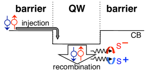
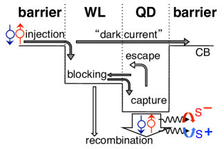
Figure 1: (Color online) Conduction band (CB) diagram and characteristic processes in semiconductor lasers. (a) Quantum well (QW) laser. A preferential spin alignment of the injected carriers, leads, through electron-hole recombination, to circularly polarized emitted light ($S^{\pm}$ are the emitted photons with positive and negative helicity, respectively). (b) Quantum dot (QD) laser contains an additional level arising from the wetting layer (WL) as well as several more processes, not present in QW lasers.

A schematic description of the QW and QD semiconductor laser is depicted in Fig. 1, representing the conduction band (CB) diagram and several characteristic processes included in our rate equation (RE) approach.Gothgen2008:APL ; Lee2010:APL ; Oszwaldowski2010:PRB With the usually employed assumption of charge neutrality, the underlying picture is simplified since holes need not be explicitly considered for conventional lasers.Gothgen2008:APL The injection of spin-polarized carriers leads to circular polarization of the emitted light.Meier:1984 ; Zutic2004:RMP ; Zutic2001:PRB ; Vulovic2011:JAP ; Iba2011:APL Depicted carrier recombination (in both QWs and QDs) is either spontaneous or stimulated, and a sufficiently high injection leads to the onset of lasing when the optical gain can overcome losses in the resonant cavity.

A more complex description of QD lasers includes several additional processes and a two-dimensional QW-like wetting layer (WL), which acts as a reservoir of carriers.Dery2005:JQE ; Fiore2007:JQE ; Summers2007:JAP Carriers from the WL are captured to the QD or, conversely, they can escape from QD to WL. To correctly describe the small density of QD states, as well as saturation of the WL states at high injection, it is important to include the Pauli blockingOszwaldowski2010:PRB ; Dery2005:JQE ; Fiore2007:JQE ; Summers2007:JAP ; Taylor2010:APL which impedes carrier transfer to states close to saturation. The Pauli blocking is responsible for additional nonlinear contributions to the QD REs and for a dark current (i.e., a current that is not accompanied by any emission of light), both of which are absent in our simpler description of QW lasers.

To provide an intuitive picture of changes arising from the spin-polarized injection, we develop here a bucket model of spin lasers, compared in Fig. 2 with the well-known model for conventional lasers.Parker:2004 A simple analogy with the pumped bucket illustrates on and off regimes in conventional lasers, where the outgoing water represents the emitted light. At low injection or pumping $J$, there is only negligible output light. The operation of a laser is similar to that of a light emitting diode (LED); the spontaneous recombination is responsible for the emitted light. At higher injection, when the water starts to gush out of the large slit in Fig. 2, the lasing threshold is reached. At the threshold injection $J_{T}$, stimulated emission starts and the emitted light intensity increases significantly. $J>J_{T}$ corresponds to lasing operation in which the stimulated recombination is the dominant mechanism of light emission.

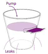
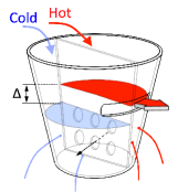
Figure 2: (Color online) Bucket model of lasers. (a) Conventional laser. Pump (injection) fills the bucket with small leaks (corresponding to spontaneous recombination and the off regime with negligible light emission) and a large slit from which, above sufficiently strong pumping, the water will gush out (corresponding to stimulated emission and the onset of lasing in the on regime). An additional increase in pumping will lead only to a small change in the water level (representing carrier density in a laser), but the output will increase rapidly, as compared to the off regime. (b) Spin laser. Two halves of the bucket, representing two spin populations (hot and cold water) are separately filled. The partition between them is not perfect: openings in the partition model the spin relaxation which mixes the two populations. The difference between uneven water levels, denoted by $\Delta$, represents the spin imbalance in the laser. Here, in addition to the on and off regimes, one can infer a regime where only hot water will gush out. This represents the spin-filtering regime between two different lasing thresholds: even a modest polarization of injection leads to complete polarization of emission.

We next turn to the pictorial representation of a simple spin laser. To model different projections of carrier spin or helicities of light, it is convenient to think of an analogy with hot and cold water, as shown in Fig. 2. The bucket is partitioned into two halves, representing two spin populations, which are separately filled with hot and cold water, respectively. The openings in the partition allow mixing of hot and cold water, intended to model the spin relaxation.Zutic2004:RMP With an unequal injection of hot and cold water, injection spin polarization is defined asnegative

$$P_{J}=(J_{+}-J_{-})/J,$$ (1)

where $J_{\pm}$ are the injections of the two spin projections which together comprise the total injection $J=J_{+}+J_{-}$. The difference in the hot and cold water levels $\Delta$ [see Fig. 2], leads to the three operating regimes and two different lasing thresholds $J_{T1,2}$.Gothgen2008:APL

At low pumping (when both hot and cold water levels are below the large slit), both spin-up and spin-down carriers are in the off (LED) regime, thus with negligible emission. At higher pumping, the hot water reaches the large slit and it gushes out as depicted in Fig. 2, while the amount of cold water coming out is still negligible. Such a scenario represents a regime in which the majority spin is lasing, while the minority spin is still in the LED regime; thus the stimulated emission is from recombination of majority spin carriers. Two important consequences of this regime are already confirmed experimentally: (i) A spin laser will start to lase at a smaller total injection than a corresponding conventional laser (only a part of the bucket needs to be filled). This represents the threshold reduction in spin lasers,Rudolph2003:APL ; Holub2007:PRL ; Gothgen2008:APL ; Vurgaftman2008:APL ; Oestreich2005:SM ; Holub2011:PRB which can be parametrized as

$$r=1-J_{T1}/J_{T},$$ (2)

where $J_{T1}$ is the majority spin threshold ($J_{T1}<J_{T}$). (ii) Even a modest injection polarization $P_{J}\ll 1$ can lead to highly circularly polarized light.Lee2010:APL ; Saha2010:PRB The relative width of this “spin-filtering regime” can be expressed as the intervalOszwaldowski2010:PRB

$$d=(J_{T2}-J_{T1})/J_{T},$$ (3)

where $J_{T2}$ is the minority spin threshold ($J_{T1}<J_{T}<J_{T2}$) and the width of this interval increases with the injection spin polarization. $J>J_{T2}$ gives rise to minority helicity photons from minority spin carriers, and the spin polarization of light converges to $-P_{J}$ with increasing injection,Gothgen2008:APL ; negative analogous to the situation where both hot and cold water gush out.

Based on the intuitive pictures that we describe here, we present the rate equations for QD and QW lasers in the following section. Solution of the REs in the steady-state and dynamic-operation regimes gives two possible approaches to the mapping. In Sec. III, we focus on the steady-state mapping while Sec. IV is dedicated to the dynamic mapping of conventional lasers. We analyze the differences between these two mapping methods in Sec. V because the two mappings are not equivalent to each other. In Secs. VI and VII, we expand the mappings to spin lasers. Finally, we summarize our work; and suggest possible directions for further research.

II Rate Equations

In this work we consider rate equations which have been successfully used to describe both conventional and spin lasers.Chuang:2009 ; Parker:2004 ; Rudolph2003:APL ; Rudolph2005:APL ; Holub2007:PRL ; Gothgen2008:APL ; Basu2008:APL ; Basu2009:PRL ; Saha2010:PRB ; Fiore2007:JQE ; Summers2007:JAP ; SanMiguel1995:PRA ; Dyson2003:JOB ; Adams2009:JQE ; Al-Seyab2011:PJ ; Gerhardt2011:APL ; Jahme2010:APL ; Dery2004:JQE An advantage of this approach is its simplicity. REs can provide a direct relation between material characteristics and device parameters,Fiore2007:JQE as well as often allowing analytical solutions and an effective method to elucidate many trends in the operation of lasers.Chuang:2009 ; Parker:2004 ; Coldren:1995 ; Gothgen2008:APL ; Lee2010:APL For conventional QW lasers, we employ the widely used REs (Ref. Chuang:2009, ) for carrier and photon density, $n$ and $S$, respectively (generalized REs for spin lasers are given in Appendix A):

$$dn/dt = J-g(n,S)S-R_{\mathrm{sp}},$$ (4)

$$dS/dt = \Gamma g(n,S)S+\Gamma\beta R_{\mathrm{sp}}-S/\tau_{\mathrm{ph}},$$ (5)

where the charge neutrality was used to eliminate the REs for holes. To describe stimulated emission, the optical gain term is usually modeled asChuang:2009

$$g(n,S)=g_{0}(n-n_{\mathrm{tran}})/(1+\epsilon S),$$ (6)

where $g_{0}$ is the gain coefficient,Holub2007:PRL $n_{\mathrm{tran}}$ is the transparency density at which the optical gain becomes zero, and $\epsilon$ is the gain compression factor.Chuang:2009 ; Lee1993:OQE The spontaneous recombination $R_{\mathrm{sp}}$ can have various density dependences; here we focus on the quadratic formChuang:2009 ; Gothgen2008:APL ; Zutic2006:PRL $Bn^{2}$, where $B$ is a temperature-dependent constant. $\Gamma$ is the optical confinement factor, arising from different volumes of the resonant cavity and the active region of the lasers;Chuang:2009 $\beta$ is the spontaneous emission factor ($\beta\rightarrow 0$ is an accurate approximation since typical experimental values $\beta\sim 10^{-5}-10^{-4}$ do not alter laser behavior significantly, but slightly complicate the definition of threshold).Gothgen2008:APL ; Lee2010:APL ; Yu:2003 The photon lifetime $\tau_{\mathrm{ph}}$ reflects optical losses such as absorption in the boundary media, photon scattering, and loss at the mirrors.Yariv:1997

To describe QD lasers, it is more appropriate to use occupancies, rather than carrier and photon densities.Fiore2007:JQE ; Summers2007:JAP The REs describing the QD-based lasers [Fig. 1] are more complex than Eqs. (4) and (5), used for QW lasers. REs for QD spin lasers are given in Appendix A. Here we explain their limiting case for conventional lasers written in an abbreviated form,

$$df_{w}/dt = I-C+\frac{2}{\kappa}E-R_{w},$$ (7)

$$df_{q}/dt = \frac{\kappa}{2}C-E-R_{q}-G,$$ (8)

$$df_{S}/dt = \Gamma_{\mathrm{QD}}G+\Gamma_{\mathrm{QD}}\beta R_{q}-f_{S}/\tau_{\mathrm{ph}},$$ (9)

where the indices $w$ and $q$ represent the WL and QD regions, while the index $S$ pertains to photons. The electron occupancies (those for holes were eliminated using charge neutrality and the assumption that the capture and escape times for the electrons and holes are equal) $0\leq f_{w,q}\leq 1$ are related to the corresponding number of electrons $\bar{n}_{w,q},$ as $f_{w}=\bar{n}_{w}/N_{w}$ and $f_{q}=\bar{n}_{q}/(2N_{q})$, where $N_{w}$ is the number of states in the WL and $N_{q}$ is the number of QDs [each dot contains a twofold- (spin-) degenerate level], related by the ratio $\kappa=N_{w}/N_{q}$. Here, we use an overbar to distinguish numbers from the corresponding densities used in Eqs. (4)-(6). The photon occupancy $f_{S}=\bar{S}/(2N_{q})$, where $\bar{S}$ is the number of cavity photons, does not have an upper bound.

The carrier injection and the capture from the WL to the QDs are $I=j(1-f_{w})$ and $C=f_{w}(1-f_{q})/\tau_{c}$, where $j$ is the number of carriers (electrons) injected into the laser per WL state and unit time, while $\tau_{c}$ is the capture time. An opposite process to the carrier capture is their escape $E=f_{q}(1-f_{w})/\tau_{e}$, where $\tau_{e}$ is the escape time. These processes have a characteristic Pauli blocking factor $(1-f)$, absent in the analysis of QW lasers, as shown in Eqs. (4) and (5). It is instructive to note the nonlinear form (in the carrier occupancies) of the escape and capture terms $E$, $C$ in QDs. The absence of such nonlinearities in QW laser REs provides another simplification in understanding QD lasers through the mapping procedure, which allows their more transparent description. Other processes depicted in Fig. 1 are the spontaneous radiative recombinations $R_{\eta}=b_{\eta}f^{2}_{\eta}$, where $\eta=w,q$. The charge neutrality implies that $f^{2}_{\eta}$ actually corresponds to the product of electron and hole occupancies.Oszwaldowski2010:PRB Coupling of carriers and light in Eqs. (8) and (9) is responsible for stimulated emission, which can be described by

$$G=g(2f_{q}-1)f_{S},$$ (10)

where $g$ is independent of photon occupancies and does not contain the gain compression factor $\epsilon$, used in the QW lasers. By using occupancies, rather than densities, for QD REs, different volume factors are eliminated and there is no need to introduce the optical confinement factor ( $\Gamma_{\mathrm{QD}}=1$), required in Eq. (5). Finally, $\tau_{\mathrm{ph}}$ is analogous to the quantity already used in Eq. (5).

III Steady-State Mapping

Based on the REs described in Sec. II, we explore the feasibility of mapping between QD and QW lasers. Our goal is to approximate the solutions for the more complicated QD laser REs by the solutions we obtain from solving REs for QW lasers. To achieve the mapping, there are two requirements for the mapped QW laser REs. First, the REs should be able to estimate steady-state properties such as threshold and light intensity with a reasonable accuracy. At the same time, the dynamic response of lasers should also be presented by the REs through various numerical or analytical methods such as large- or small-signal analyses. In this section, as the first step, we focus on the steady-state operation for which the QW mapping parameters are extracted from the QD parameters by solving Eqs. (4), (5) and (7)-(9) analytically, while the constants $\tau_{\mathrm{ph}}$ and $\beta$ are kept the same for QD and QW lasers. This mapping corresponds to the situation in which the active region comprised of QDs and WLs is considered as QWs, while retaining the remaining geometry of the laser. Ideally, the following equations should hold:

$$J = \kappa(N_{q}/V)j,$$ (11)

$$n(J) = (N_{q}/V)[2f_{q}(j)+\kappa f_{w}(j)],$$ (12)

$$S(J) = 2\Gamma(N_{q}/V)f_{S}(j),$$ (13)

where $N_{q}$ and $\kappa$ were previously defined, $V$ is the volume of the active region, and $J$ ($j$) represents injection in the QW (QD) laser REs. While Eq. (11) holds by definition, Eqs. (12) and (13) can not be satisfied for all $j$’s. Therefore we impose four matching points where the two solutions from QW and QD laser REs should coincide:

(i) Transparency carrier density $n_{\mathrm{tran}}=(N_{q}/V)[2f_{q}(j_{\mathrm{tran}})+\kappa f_{w}(j_{\mathrm{tran}})]$, where $n_{\mathrm{tran}}=n(J_{\mathrm{tran}})$, and $J_{\mathrm{tran}}$ and $j_{\mathrm{tran}}$ are the injection values at transparency satisfying $f_{q}(j_{\mathrm{tran}})=1/2$ [see Eqs. (6) and (10)].

(ii) Threshold carrier density $n_{T}=n_{\mathrm{tran}}+1/(\Gamma g_{0}\tau_{\mathrm{ph}})=(N_{q}/V)[2f_{q}(j_{T})+\kappa f_{w}(j_{T})]$ determines $g_{0}$ (for QW lasers), where $j_{T}$ is the injection (for QD lasers) at threshold.

(iii) Threshold current density $J_{T}=Bn_{T}^{2}=\kappa(N_{q}/V)j_{T}$ determines $B$ (for QW lasers), where $j_{T}$ is the QD laser threshold injection current.

(iv) Photon density $S=2\Gamma(N_{q}/V)f_{S}$ determines $\epsilon_{s}$, where the subscript $s$ denotes that it was obtained in the steady-state (static) case. At a fixed injection ($J=\alpha J_{T}$ or $j=\alpha j_{T}$), the photon densities obtained from QD and QW laser REs are made to coincide. In this paper, $\alpha=10$ is used.

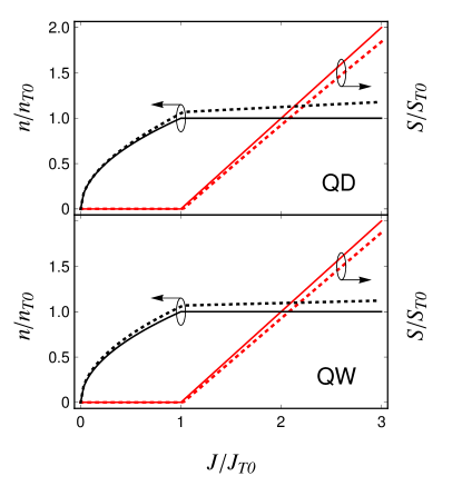
Figure 3: (Color online) Carrier ($n$) and photon densities ($S$) as functions of injection $J$. $n$ and $J$ are normalized to their threshold values $n_{T0}$ and $J_{T0}$ for capture time $\tau_{c}=0$ (QD lasers) or gain compression factor $\epsilon_{s}=0$ (QW lasers), while $S$ is normalized to $S_{T0}\equiv S(2J_{T0})$. For QD lasers, solid and broken lines represent $\tau_{c}=0$ and $\tau_{c}=2$ ps, while they represent $\epsilon_{s}=0$ and $1.62\times 10^{-14}~{}$cm³ for QW lasers. Note that QW laser characteristics for $\epsilon_{s}=0$ are identical to QD laser characteristics for $\tau_{c}=0$. The mapping parameters used throughout this paper are given in Table 1.

Table 1: Mapping parameters. The QD parameters are $\tau_{\mathrm{ph}}=2$ ps, $b_{q}\tau_{\mathrm{ph}}$=0.01, $b_{w}\tau_{\mathrm{ph}}$=2.33, $g\tau_{\mathrm{ph}}=2$, $\kappa$=100 and $\tau_{e}$=1 ns (Ref.  Fiore2007:JQE, ; Ezra2009:JQE, ; Erneus2007:PRA, ; Rsp:comment, ).

QW param.	$\tau_{c}=0$	$\tau_{c}=2$ ps	unit
$\epsilon_{s}$	0	$1.62\times 10^{-14}~{}$	cm3
$\epsilon_{d}$ (Ref. sec:DOM, )	0	$6.39\times 10^{-15}~{}$	cm3
$g_{0}$	1.90 $\times 10^{-3}$	1.65 $\times 10^{-3}$	cm3s-1
$n_{\mathrm{tran}}$	$3.50\times 10^{16}$	$3.58\times 10^{16}$	cm-3
$B$	$1.43\times 10^{-7}$	$1.28\times 10^{-7}$	cm3s-1
$\tau_{\mathrm{ph}}$	2		ps
$\Gamma$	0.03
$\beta$	0

Results of the above mapping are shown in the Fig. 3, comparing the light-injection and carrier-density-injection characteristics for QD and QW lasers for different $\tau_{c}$’s. The corresponding mapping parameters are given in Table 1. In the limit of $\tau_{c}\to 0$, the wetting layer is “transparent” to carriers, since injected carriers are immediately captured into QDs; therefore, within the RE description for $\epsilon_{s}=0$, QD and QW lasers behave identically. In both cases, when $\tau_{c}=0$ or $\epsilon_{s}=0$, the carrier density (black solid) is pinned (fixed) above the threshold and the photon density increases linearly, as expected.Chuang:2009 ; Saha2010:PRB

For finite $\tau_{c}$ (2 ps in Fig. 3) the carrier density is enhanced and the photon density is suppressed. For $n>n_{T}$ the increase in carrier density can be mostly attributed to WL occupancy, which increases for $\tau_{c}>0$. Without any gain term in Eq. (7), we can infer that the WL occupancy does not contribute to stimulated emission. However, since the active region is considered as comprised of QDs and the WL, we take into account this “inefficiency” of the WL for light emission by introducing $\epsilon_{s}$ in the QW laser model. The typical range of $\epsilon$ experimentally obtained in QW lasersHolub2007:PRL ; Rudolph2003:APL is $\epsilon\sim 10^{-19}-10^{-17}$. In contrast, in our mapping we employ (Table 1) a much larger $\epsilon_{s}\sim 10^{-14}$, which captures well the behavior of QD lasers, as can be seen by comparison of the upper and lower panels in Fig. 3. The analysis of Fig. 3 reveals that in a QD laser the effect of finite $\tau_{c}$ (i.e., to increase $n$ and suppress $S$ with injection) is similar to the influence of a finite gain compression factor $\epsilon_{s}$ in a QW laser. This suggests that, in the steady state, by finding $\epsilon_{s}$ as a function of $\tau_{c}$, QD laser REs can be accurately replaced by QW laser REs. It is also instructive to note that as $\tau_{c}$ becomes longer in QD lasers, parasitic effects such as spectral hole burning or phonon bottleneck will arise, and these nonlinear effects are taken into account by introducing $\epsilon$ in QW laser REs.

IV Dynamic-Operation Mapping

The mapping between QD and QW lasers works well in the steady state, and the influence of finite $\tau_{c}$, as shown in Fig. 3, on light-injection and even carrier-density-injection characteristics is accurately modeled by introducing a large $\epsilon_{s}$ in the QW laser. However, the most useful properties of lasers typically pertain to their dynamic operation, and it is important to understand if in this case the mapping proposed above is still relevant. To address this, we consider the standard approach of small-signal analysis (SSA),Chuang:2009 and apply it to both QD and QW lasers. We decompose the quantities of interest, $X$, into a steady-state $X_{0}$ and a (small) modulated part $\delta X(t)$, $X=X_{0}+\delta X(t)$, and focus on the harmonic modulation $\delta X(t)=\mathrm{Re}[\,\delta X(\omega)e^{-i\omega t}]$, where $\omega$ is the (angular) modulation frequency. The response function, which characterizes the dynamic operation including the laser bandwidth, an important figure of merit, is given by

$$R(\omega)=\left|\delta S(\omega)/\delta J(\omega)\right|.$$ (14)

It is convenient to consider the normalized frequency response functionChuang:2009

$$\left|\frac{R(\omega)}{R(0)}\right|_{\mathrm{QW}}=\frac{\omega_{R}^{2}}{[(\omega_{R}^{2}-\omega^{2})^{2}+\omega^{2}\gamma^{2}]^{1/2}},$$ (15)

where $\omega_{R}^{2}\approx g_{0}S_{0}/\left[\tau_{\mathrm{ph}}(1+\epsilon S_{0})\right]$ is the relaxation oscillation frequency, and $\gamma$ is a damping factor.Fowles:2005 ; wR The functional form of Eq. (15) is the same as for amplitude of a harmonically-driven damped harmonic oscillator.Fowles:2005 It is useful to express the damping factor as

$$\gamma\approx 2Bn_{T}+K\,[\omega_{R}^{2}/(2\pi)]^{2},$$ (16)

where the $K$-factor

$$K \approx 4\pi^{2}\left(\tau_{\mathrm{ph}}+\epsilon/g_{0}\right)$$ (17)

is an important characteristic parameter that determines the high-speed operation limit of lasers. In the above equations, we assume $\epsilon\ll g_{0}/(2Bn_{T})$; the exact forms are given in Appendix B.

The bandwidth of the laser, $\omega_{\mathrm{3dB}}$ (see Appendix B), is the frequency at which the square of $|R(\omega)/R(0)|$ in Eq. (15) is reduced by 3 dB. $\omega_{\mathrm{3dB}}$ and $\omega_{R}$ are functions of the steady-state injection $J_{0}$, and they coincide for the maximum bandwidth $\omega_{\mathrm{3dB}}^{\mathrm{max}}$. Commonly, the peak position $\omega^{2}_{\mathrm{peak}}=\omega_{R}^{2}-\gamma^{2}/2$ in the response function is approximated as $\omega_{R}$ (when $\omega_{R}\gg\gamma$, i.e., weak damping), while the bandwidth in QW lasers can be related to $\omega_{\mathrm{peak}}$ and $\omega_{R}$,Coldren:1995 ; Asryan2010:APL

$$\omega^{2}_{\mathrm{3dB}}=\omega^{2}_{\mathrm{peak}}+(\omega_{\mathrm{peak}}^{4}+\omega_{R}^{4})^{1/2}.$$ (18)

The maximum bandwidth is attained for $\omega_{R}^{2}=\gamma^{2}/2$ to give a monotonic decrease of response function defined in Eq. (15).

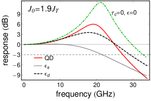
Figure 4: (Color online) Small-signal analysis for QD and QW lasers, given by the square of the normalized frequency response function. The solid line represents QD laser response ($\tau_{c}=2$ ps; see Table 1), while for QW lasers, the dashed and dotted lines correspond to static and dynamic gain compression factors $\epsilon_{s}=1.62\times 10^{-14}$ cm³ and $\epsilon_{d}=6.39\times 10^{-15}$ cm³, respectively. The response for $\epsilon=0$ (dot-dashed), identical to the response of the QD laser for $\tau_{c}=0$, is shown for comparison.

For QD lasers the response function can be related to its QW counterpart in Eq. (15), under the assumption of $\omega_{r}^{\prime}\ll 1/\tau_{c}^{\prime}$, where $\omega_{r}^{\prime}$ ($\gamma_{\mathrm{QD}}$) for a QD laser corresponds to $\omega_{R}$ ($\gamma$) for a QW laser, and $\tau_{c}^{\prime}\approx\tau_{c}/(1-f_{q0})$ is the effective capture time. In this regime, often realized experimentally, we obtain (more general expressions are given in Appendix B)

$$\left|\frac{R(\omega)}{R(0)}\right|_{\mathrm{QD}}\approx(1+\omega^{2}\tau_{c}^{\prime 2})^{-1/2}\times\left|\frac{R(\omega)}{R(0)}\right|_{\mathrm{QW}}.$$ (19)

Analogously to QW lasers, the bandwidth for QD lasers can be obtained from the equation

$$(1+\omega_{\mathrm{3dB}}^{2}\tau_{c}^{\prime 2})[(\omega_{r}^{\prime 2}-\omega_{\mathrm{3dB}}^{2})^{2}+\omega_{\mathrm{3dB}}^{2}\gamma_{\mathrm{QD}}^{2}]=2\omega_{r}^{\prime 4},$$ (20)

which in the limit of $\tau_{c}\to 0$, recovers the QW behavior, determined by Eq. (18). Our REs for the QD laser resemble those for separate confinement heterostructure (SCH) lasers,Nagarajan1992:JQE except that for QD lasers it is important to consider the Pauli exclusion principle. The Pauli factor, which appears in the form of $1-f_{\eta}$, not only reduces the steady-state photon density, but also significantly suppresses the modulation response. Similarly to the corresponding capture in SCH lasers,Chuang:2009 the contribution of $\tau_{c}$ to the QD modulation response function is responsible for low-frequency roll-off (i.e., negative slope of the response). When $\tau_{c}$ is so large that the roll-off is dominant, the maximum bandwidth attained is $\sim 1/\tau_{c}^{\prime}$. Our results imply that to maximize the QD laser dynamic response, the capture time should be sufficiently short, $\tau_{c}<10$ ps, consistent with a previous study of QDs.Ohnesorge1996:PRB ; Heitz1997:PRB ; Sugawara1997:APL ; Muller2003:APL ; Ishida2004:APL As mentioned in Sec. III, it is required that the mapped QW laser REs recover the dynamics of QD lasers.

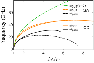
Figure 5: (Color online) Injection dependence of characteristic frequencies obtained from small signal analysis: Gray (orange) and black lines show bandwidth ($\omega_{\mathrm{3dB}}$) and peak frequency ($\omega_{\mathrm{peak}}$), respectively. Solid and dashed lines represent QW and QD lasers, respectively. The dotted line is the bandwidth of a mapped QW laser for $\epsilon=0$.

While our goal is not to fully recover a detailed dynamic response of QD lasers, we do require that the maximum bandwidth $\omega_{\mathrm{3dB}}^{\mathrm{max}}$, as the key figure of merit characterizing dynamical operation, coincides for QD and QW lasers. This can be achieved through a $K$-factor that defines the maximum frequency for QW lasers and depends on $\epsilon$. The mapping is then realized by following the same matching procedure and conditions (i)-(iii) described in Sec. III, while for the previous condition (iv) is now replaced by the expression for $\epsilon_{d}$ which reflects the matching of the maximum bandwidth from Eq. (17),

$$\epsilon_{d}\approx g_{0}\left(\sqrt{2}/\omega_{\mathrm{3dB}}^{\mathrm{max}}-\tau_{\mathrm{ph}}\right),$$ (21)

where the subscript $d$ refers to the dynamical response with the corresponding value which does not need to coincide with the value obtained in the steady-state mapping, i.e., $\epsilon_{s}$. The maximum bandwidth $\omega_{\mathrm{3dB}}^{\mathrm{max}}$ is obtained from the QD laser REs; Eq. (21) is valid for $\omega_{\mathrm{3dB}}^{\mathrm{max}}\gg 2Bn_{T}$ and $\epsilon_{d}\ll g_{0}/(2Bn_{T})$. Equation (21) gives a less than 3% error with $\tau_{c}=2$ ps, compared to exact calculation [see Eq. (37) in Appendix B]; however, for mapping over a wide range of $\tau_{c}$, we used the general expressions presented in Appendix B.

To examine differences between the two mapping procedures, in Fig. 4 we compare the response function of a QD laser to response functions calculated for QW lasers from both steady-state and dynamical-response mapping at a given injection ($J_{0}=1.9J_{T}$). In the limit $\tau_{c}=0$, REs for QD lasers reduce to REs for QW lasers with $\epsilon=0$. We see qualitative similarities for finite $\epsilon$ and $\tau_{c}$ which are both detrimental and cause bandwidth suppression. In small-signal analysis, the calculated QW laser response function shows a wider spread and different slope in the tail than the one for QD lasers. As can be seen from Fig. 4, use of the gain compression factor obtained from the steady-state mapping, $\epsilon_{s}$, provides a poor approximation to the response function for a QD laser. The agreement is considerably better when a much smaller gain compression factor from dynamical-operation mapping, $\epsilon_{d}$, is used instead. We see that the QD and QW response functions are nearly indistinguishable up to $\sim$ 10 GHz (the maximum bandwidths are matched for higher currents).

To assess the quality of the dynamic-operation mapping, in Fig. 5 we show the injection dependence of the bandwidth $\omega_{\mathrm{3dB}}$ and the peak position $\omega_{\mathrm{peak}}$ for the QD and QW lasers. It is remarkable that the mapping, only intended to match the maximum bandwidth between the QD and QW lasers, yields a very good agreement for the bandwidth dependence on injection. Both QD and QW cases reveal a nonmonotonic behavior up to $J\sim 6J_{T0}$. While Fig. 4 shows a very similar peak position for QD and QW lasers, from Fig. 5 we can infer that this occurs typically only close to the threshold injection. The discontinuity of $\omega_{\mathrm{peak}}$ for the QD laser (black solid curve) is due to low-frequency roll-off. As a result of the interplay of $\tau_{c}^{\prime}$ and $\omega_{r}^{\prime}$, shown in Eq. (20), $\omega_{\mathrm{peak}}=0$ (analogous to an overdamped harmonic oscillatorFowles:2005 ) only above injection $J_{0}\sim 5.7J_{T}$.

V Steady-State vs Dynamic-Operation Gain Compression

In the preceding two sections we have formulated steady-state and dynamic-operation mapping and showed that, with the corresponding change in $\epsilon$, there are considerable differences when it comes to small-signal analysis. We now examine if these differences, between choice of $\epsilon_{s}$ and $\epsilon_{d}$, also persist in the steady-state regime. In Fig. 6 we consider light-injection and carrier density-injection characteristics.

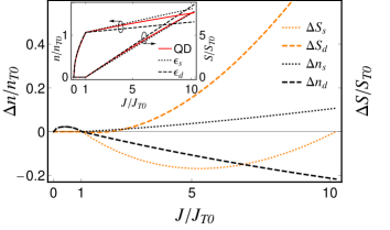
Figure 6: (Color online) Deviations of QD laser photon ($\Delta S$) and carrier ($\Delta n$) densities from those obtained by mapped QW lasers with $\epsilon_{s}$ (dotted) and $\epsilon_{d}$ (dashed). Black [gray (orange)] lines are deviations in carrier (photon) densities (same scale as for $\Delta n/n_{T0}$). Note that $10J_{T}\approx 10.23J_{T0}$. Inset: Carrier and photon densities for QD and QW lasers with $\epsilon_{s}$ and $\epsilon_{d}$ are shown by solid, dotted, and dashed lines, respectively. Note the different vertical scales.

The light intensity at $J=10J_{T}$ for QW laser dynamic mapping ($\epsilon_{d}$) is about 10 $\%$ higher than for QD and QW lasers steady-state mapping ($\epsilon_{s}$). The light intensity at $J=10J_{T}$ is set to be the same for QD and QW laser with $\epsilon_{s}$ chosen according to the matching condition (iv) in Sec. III. The carrier density of the QW lasers is noticeably different from the of the QD laser. Typically the relative differences in carrier density are more pronounced than in the light intensity (see Fig. 6 inset). Since, generally, $\epsilon_{s}>\epsilon_{d}$, a higher light intensity is maintained for $\epsilon_{d}$ at the same injection by consuming more carriers in the active region through stimulated recombination. Therefore, at $J=10J_{T}$, the carrier density of QW lasers with $\epsilon_{d}$ (gray solid) is about 30 $\%$ lower than that of QW lasers with $\epsilon_{s}$ (black solid).

Recognition of the correspondence between the increasing capture time in QD lasers and the increasing gain compression factor in QW lasers was the basis for both the steady-state and dynamic mapping. In the previous plots (see Figs. 3 and 4) we focused on a modest capture time ($\tau_{c}=2$ ps). In Fig. 7, $\epsilon_{s}$ and $\epsilon_{d}$ of mapped QW lasers are plotted as functions of capture time of QD lasers, for different gain coefficients.

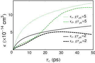
Figure 7: (Color online) Gain compression factors $\epsilon_{s}$ (dotted) and $\epsilon_{d}$ (dashed), obtained from two different mapping procedures. Thick (black) and thin [gray(green)] lines represent $g\tau_{\mathrm{ph}}=2$ and 5, respectively, for $\tau_{\mathrm{ph}}=2$ ps.

These results show that, when the two mappings are compared, $\epsilon_{s}$ is always greater than $\epsilon_{d}$, which leads to an excessive suppression of dynamic response when the steady-state mapping of QD lasers is implemented. While $\epsilon_{s}$ shows a monotonic increase with $\tau_{c}$, there is a nonmonotonic variation of $\epsilon_{d}$. In particular, $\epsilon_{d}$ has a local maximum at $\tau_{c}\sim 30$ (43) ps for $g\tau_{\mathrm{ph}}=2$ (5) and starts to decline for large $\tau_{c}$. This unexpected behavior of $\epsilon_{d}$ reflects a rapid decrease of the mapped QW laser gain $g_{0}$. The maximum bandwidth $\omega_{\mathrm{3dB}}^{\mathrm{max}}$ of a QD laser decreases with increasing $\tau_{c}$, and in maintaining the same value of $\omega_{\mathrm{3dB}}^{\mathrm{max}}$ within QW laser REs, $\epsilon_{d}$ and $g_{0}$ play an important role. As $\tau_{c}$ grows, $g_{0}$ and $B$ respectively decline and increase according to the conditions (ii) and (iii) in Sec. III. Beyond $\tau_{c}\sim 30$ (43) ps, $\omega_{\mathrm{3dB}}^{\mathrm{max}}$ tends to saturate to $2Bn_{T}$, while the decrease of gain retains its rate. As a result, $\epsilon_{d}$ has to stop rising and even starts to decrease with $\tau_{c}$ to compensate for the rapidly diminishing gain, leading to the maximum of $\epsilon_{d}$ in Fig. 7.

VI Mapping of Spin Lasers

Our preceding analysis of mapping was limited to the absence of injected spin polarization ($P_{J}=0$). The more general case of spin lasers ($P_{J}\neq 0$) adds complexity to REs, requiring four equations for QW and ten for QD lasers (see Appendix A). For QDs, the added complexity prevents analytical solutions even in the steady state, making any attempt at directly implementing the mapping for spin lasers more challenging. On the other hand, this same complexity implies that the prospect of studying QD spin lasers by considering a simpler description for QW spin lasers will be more valuable than in the conventional lasers. Moreover, important recent experiments on QD-based spin lasersBasu2008:APL ; Basu2009:PRL ; Saha2010:PRB are described within the formalism of QW spin laser REs and it is not a priori clear how accurate is such a procedure. Typically, these spin lasers are realized in a Faraday geometryZutic2004:RMP as vertical-cavity surface-emitting lasers (VCSELs).Yu:2003 The main difference from commercially available VCSELs is the presence of spin-polarized carriers, provided by pumping with circularly polarized light or using magnetic contacts for electrical spin injection.Rudolph2003:APL ; Rudolph2005:APL ; Holub2007:PRL ; Gerhardt2011:APL ; Hovel2008:APL ; Jahme2010:APL ; Hovel2007:PSS ; Ando1998:APL ; Hallstein1997:PRB ; Soldat2011:APL ; Fraser2010:APL

In spin lasers we consider spin-resolved quantities to model different spin projections or helicities of light. The total electron or hole density can be written as the sum of the spin-up (+) and the spin-down ($-$) electron or hole densities, $n=n_{+}+n_{-}$ and $p=p_{+}+p_{-}$. Analogously, we write the total photon density as the sum of the positive (+) and negative ($-$) helicities, ${S{\,}={\,}S^{+}{\,}+{\,}S^{-}}$. A generalization of the optical gain term in Eq. (6) for QW spin lasers can be expressed as

$$g_{\pm}(n_{\pm},S^{\pm})=g_{0}(n_{\pm}+p_{\pm}-n_{\mathrm{tran}})/(1+\epsilon^{\pm}_{+}S^{+}+\epsilon^{\pm}_{-}S^{-}),$$ (22)

where $g_{\pm}$ is the spin dependent gain which couples to the corresponding spin of carriers $n_{\pm}$. The superscript of $\epsilon$ represents the spin of coupled carriers, while the subscript represents the corresponding helicity of photons. Due to the symmetry, $\epsilon_{+}^{-}=\epsilon_{-}^{+}=\epsilon_{\mathrm{cross}}$ and $\epsilon_{+}^{+}=\epsilon_{-}^{-}=\epsilon_{\mathrm{self}}$. The index cross (self) implies a cross- (self-) compression mechanism of gain. Later in this section (Fig. 9), we compare the self-compression limit ($\epsilon_{\mathrm{self}}=2\epsilon$, $\epsilon_{\mathrm{cross}}=0$ ) to the even-compression limit ($\epsilon_{\mathrm{self}}=\epsilon_{\mathrm{cross}}=\epsilon$). Each case recovers the spin-unpolarized laser REs for $P_{J}=0$.

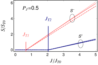
Figure 8: (Color online) Photon densities of the spin laser are shown for injection $P_{J}=0.5$. Solid, dashed, and dotted lines represent QD and QW lasers with $\epsilon_{d}$ and $\epsilon_{s}$ (given in Table 1), while gray and black lines represent left ($S^{-}$) and right ($S^{+}$) circular polarization, respectively. $S$ and $J$ are normalized to the values $S_{T0}$ and $J_{T0}$ for $P_{J}=0$ and $\tau_{c}=0$ ($\epsilon=0$). Vertical lines indicate thresholds for majority ($J_{T1}$) and minority ($J_{T2}$) spin carriers.

To establish a connection between QD and QW spin lasers, we reconsider our mapping procedure discussed above for $P_{J}=0$. We focus on the regime of a strong electron-hole spin asymmetry, shown to lead to maximum threshold reductionGothgen2008:APL ; Vurgaftman2008:APL and desirable dynamical properties of spin lasers,Lee2010:APL in which the spin relaxation time of holes is much shorter than for the electrons. For example, in bulk GaAs at room temperature the measured spin relaxation time of holes is $\sim 100$ fs,Zutic2004:RMP and of electrons it is $\sim 0.1-1$ ns.Fabian2007:APS In spin lasers it is therefore customary to consider that holes are spin unpolarized. Here, for simplicity, we also focus mostly on the infinitely long spin relation times for electrons (in the QW, WL, and QD regions). This limiting case can accurately describe recent experiments,Fujino2009:APL ; Ikeda2009:PTL in which the spin relaxation time for electrons is not only much longer than for holes, but also much longer than the other characteristic timescales for the carriers.

The light-injection characteristics obtained for mapping of QD to QW spin lasers with self-compression are shown in Fig. 8. Several key features of spin lasers that can already be inferred from the bucket model in Fig. 2 are clearly present. With $P_{J}\neq 0$ the thresholds for majority and minority spin ($J_{T1}$ and $J_{T2}$) are different. Since $J_{T1}<J_{T}<J_{T2}$ there is a threshold reduction $r$ [recall Eq. (2)], as compared to conventional lasers. Furthermore, for injection $J_{T1}<J<J_{T2}$ there will be a spin-filtering effect [Eq. (3)]; even a modest injection leads to fully polarized emitted light.Lee2010:APL ; Saha2010:PRB Even though our results have been based on parameters identical to the ones used for conventional lasers (supplemented by the vanishing hole and infinite electron spin relaxation times), we retain a good agreement between QD and QW lasers, especially near the two thresholds. For example, in Fig. 8 within dynamical mapping determined by $\epsilon_{d}$, the emitted right circular polarization, $S^{+}$ [black(blue) dashed line] is almost indistinguishable for QD and QW lasers.

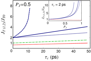
Figure 9: (Color online) First [gray(red)] and second [black(blue)] thresholds as functions of capture time $\tau_{c}$ for $P_{J}=0.5$. Solid lines represent the QD spin laser, while dotted and dashed lines correspond to QW spin lasers with self- and even- compression of gain, respectively. For comparison, the threshold of a conventional QD laser ($P_{J}=0$) is shown by the dot-dashed line. Inset: The thresholds as functions of injection polarization $P_{J}$ for $\tau_{c}=2$ ps.

We further explore the mapping of spin lasers in Fig. 9; the inset shows the evolution of majority and minority thresholds with injection polarization, for both even- and self-compression of gain. There is an excellent agreement of $J_{T1}$ for all $P_{J}$’s (the three curves overlap) and a good agreement of $J_{T2}$ up to $P_{J}\sim 0.6$, which implies that, within practical injection polarization of spin lasers realized at room temperatures, the proposed mapping works well. From the dependence of $J_{T2}$ on $P_{J}$ in QD lasers we see that their behavior falls between those of the QW approximations using self-compression only and even-compression. The same trend, i.e., $J_{T2}$ of a QD being bounded by the two limiting cases for the gain compression of QW lasers, is also shown in the main panel as a function of $\tau_{c}$ at fixed $P_{J}$. The threshold $J_{T2}$ in QW lasers disappears for the even-compression approximation, as can be seen both in the inset ($P_{J}\approx 0.83$) and in the main panel ($\tau_{c}\approx 10$ ps). In contrast, there is no disappearance of $J_{T2}$ for QW lasers with self-compression. The high accuracy of $J_{T1}$ mapping is not limited to the specific approximation of gain compression (it is independent of $\epsilon$) and persists for a wide parameter range (in both $P_{J}$ and $\tau_{c}$). As a consequence, the threshold reduction [Eq. (2)] of QD lasers is well approximated by mapping to QW lasers. The spin-filtering regime, given by Eq. (3), is present in both QD and QW lasers, but its dependence on $J_{T2}$ implies less accuracy at higher values of $P_{J}$ and $\tau_{c}$, while the latter range is experimentally less relevant. We note that in Fig. 9, only $\epsilon_{s}$ is used for the calculation since the results are insensitive to the difference between $\epsilon_{s}$ and $\epsilon_{d}$. As mentioned above, $J_{T1}$ is independent of $\epsilon$, and the difference in $J_{T2}$ due to the discrepancy between $\epsilon_{s}$ and $\epsilon_{d}$ is less than 2%.

VII Small-Signal Analysis for Spin-Lasers

Motivated by the early steady-state experiments on spin lasers, it was predicted that the observed threshold reduction could also lead to desirable dynamic operation and the bandwidth enhancement.Lee2010:APL ; Banerjee2011:JAP Recent advances in electrical and optical spin injectionSaha2010:PRB ; Fujino2009:APL ; Ikeda2009:PTL ; Iba2010:APL ; Bull2004:PSPIE ; Hanbicki2003:APL ; Salis2005:APL ; Zega2005:PRL ; Crooker2009:PRB ; Li2009:APL suggest versatile opportunities for the modulation of spin lasers. In previous work on QW spin lasers we considered amplitude and polarization modulation (AM, PM).Lee2010:APL

AM for a steady-state polarization implies $J_{+}\neq J_{-}$ (unless $P_{J}=0$ when AM recovers its standard form for conventional lasers),

$$\mathrm{AM}:\>J=J_{0}+\mathrm{Re}[\,\delta J(\omega)e^{-i\omega t}],\quad P_{J}=P_{J0}.$$ (23)

As in the steady-state analysis, $P_{J}\neq 0$ leads to unequal threshold currents $J_{T1}$ and $J_{T2}$, apparent already from the bucket model in Fig. 2. Such a modulation can be contrasted with PM, which also has $J_{+}\neq J_{-}$, but $J$ remains constant:const

$$\mathrm{PM}:\>J=J_{0},\quad P_{J}=P_{J0}+\mathrm{Re}[\,\delta P_{J}(\omega)e^{-i\omega t}].$$ (24)

It was recently shown that a similar PM scheme could enable high-performance spin-communication schemes with an effective information transfer rate that exceeds currently available realizations by several orders of magnitude.Dery2011:APL

We generalize the small-signal analysis outlined in Sec. IV and compare our results for conventional lasers with those for spin lasers, using $\epsilon_{d}$ and self-compression. The response function can be generalized as $R_{\pm}(\omega)=|\delta S^{\mp}(\omega)/\delta J_{\pm}(\omega)|$ for spin lasers and it reduces to $R(\omega)$ for $P_{J0}=0$ (AM). In Fig. 10, we consider both AM and PM, choosing $P_{J}=0.5$ and the injection $J_{T1}<J_{0}=1.9J_{T}<J_{T2}$, which lies in the spin-filtering regime. As in the previous studies of QW spin lasers, we see that both AM and PM can lead to enhanced bandwidth ($\omega_{\mathrm{3dB}}$), as compared to conventional lasers (birefringence in spin lasers could provide additional paths to enhanced bandwidthsGerhardt2011:APL ; Jahme2010:APL ).

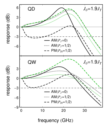
Figure 10: (Color online) The square of the normalized frequency response function of QD (upper) and QW (lower) spin lasers. Solid, dashed, and dotted lines represent amplitude modulation (AM) for $P_{J0}=0$ and $0.5$ and polarization modulation (PM) for $P_{J0}=0.5$, respectively. Injection $J_{0}$ is fixed at $1.9J_{T}$. Gray (green) lines represent finite electron spin relaxation time $tau_{s}=200$ ps for AM (dotted) and PM (dashed), respectively.

The shape of the frequency response of spin lasers in Fig. 10 is significantly modified from what was previously obtained in Ref. Lee2010:APL, due to the large $\epsilon_{d}$. This is particularly pronounced for PM, which shows a low-frequency roll-off. Despite the fact that the maximum $\omega_{\mathrm{3dB}}$ for a spin laser is enhanced, the useful frequency range for PM may be reduced due to the low-frequency roll-off before the response peak. From Fig. 10 we see that the dynamic mapping of spin lasers preserves qualitative features of the frequency response, and thus insight into the QD spin lasers can be sought from the much simpler QW REs.

VIII conclusions

We have formulated a systematic approach which allows mapping of QD to QW lasers and thus reduces the complexity of the QD laser description based on rate equations. The key observation to establish this mapping is that the influence of finite $\tau_{c}$ on the operation of QD lasers can be approximated well by a suitable choice of the gain compression factor $\epsilon$ in the simpler QW lasers.

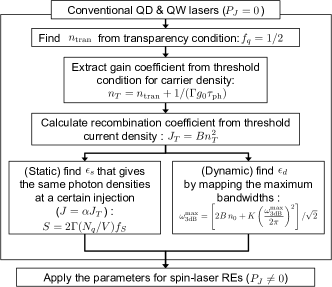
Figure 11: Schematic representation of the mapping.

However, the choice of how $\tau_{c}$ should be related to $\epsilon$ is not unique; we find noticeable differences between the mappings of either steady-state or dynamic operation of lasers, corresponding to the respective values of the gain compression factors $\epsilon_{s}$ and $\epsilon_{d}$. The mapping procedure, schematically outlined in the Fig. 11, can be realized either analytically or numerically. The steady-state mapping preserves well the behavior of a QD laser near its threshold, for both conventional and spin lasers. In the latter case, for an arbitrary injection spin polarization, the majority threshold is particularly accurate, further justifying the use of QW spin lasers REs for threshold reduction.Rudolph2003:APL ; Holub2007:PRL ; Gothgen2008:APL ; Oszwaldowski2010:PRB ; Vurgaftman2008:APL . When the dynamic-range mapping is considered, we focus on preserving the maximum bandwidth of QD and QW lasers, since their detailed behavior can display considerable differences, including low-frequency roll-off in the modulation response.Fathpour2005:JPD Additional motivation for this approach is that the bandwidth itself depends on the injection level and therefore it would not be as useful as a quantity to be matched in the mapping.

The growing interest in QD lasers and the increasing number of materials used for the active region [such as colloidal QDs (Refs. Klimov2007:N, ; Scholes2008:AFM, ; Beaulac2008:AFM, ; Stern2005:PRB, )] provides a further motivation to construct a mapping discussed in this work. Since the mapping is not limited to conventional lasers, it can also be used to guide further developments of QD spin lasers. The presence of QDs in the active region leads to reduced influence of the spin-orbit coupling,Fabian2007:APS resulting in a longer spin relaxation time which improves lasing properties, giving a lower threshold and enhanced bandwidth. Detailed knowledge of the structures used in recent experiments on QD spin lasers,Basu2008:APL ; Basu2009:PRL ; Saha2010:PRB would allow us to apply the mapping outlined above and examine how it is related to a description based on densities rather than occupancies.Saha2010:PRB

Several assumptions of the present mapping could be relaxed. To allow a more general RE description of QD lasers, it might be possible to include explicitly a finite gain compression factor into QD laser REs.Qasaimeh2009:JLT The expected change in the mapping procedure would be an appropriately rescaled (enhanced) $\epsilon$ for QW lasers, playing the combined role of the $\epsilon$ of the QD lasers and the finite $\tau_{c}$. With further studies of self- and even-compression mechanisms, it would be possible to more accurately model the gain compression with appropriately weighted contributions of the two mechanisms (reflected in the matrix structure of $\epsilon_{\pm}^{\pm}$). Future generalizations of the mapping procedure could also consider finite spin relaxation times of holes. While the spins of holes in bulk GaAs at 300 K can very accurately be treated as being lost instantaneously (approximately 3-4 orders of magnitude faster than the spin of electrons),Zutic2004:RMP in QDs the asymmetry of spin relaxation times for electrons and holes should be reduced.Fabian2007:APS

In a future work it would also be interesting to explore other forms of mapping procedures that could establish similarities between spin lasers and phase transitions in magnetic systems. Such a consideration would generalize what is already known for conventional lasers, linked to Ising ferromagnets,Degiorgio1970:PRA ; Degiorgio1976:PT and explain how the spin imbalance inherent to spin lasers can, through suitable mapping, be related to a more complex magnetic behavior.

IX Acknowledgments

This work was supported by the NSF-ECCS 1102092, NSF-ECCS CAREER, U.S. ONR, AFOSR-DCT, DOE-BES, NSF-NRI NEB 2020, and SRC. We thank H. Dery for valuable discussions.

Appendix A

For QW spin lasers, the REs given by Eqs. (4) and (5) are generalized as

$$dn_{\pm}/dt = J_{\pm}-g_{\pm}(n_{\pm},S^{\mp})S^{\mp}-R^{\pm}_{\mathrm{sp}}\mp F,$$ (25)

$$dS^{\mp}/dt = \Gamma g_{\pm}(n_{\pm},S^{\mp})S^{\mp}+\Gamma\beta R^{\pm}_{\mathrm{sp}}-S^{\mp}/\tau_{\mathrm{ph}},$$

where the $+/-$ subscript (superscript) represents the corresponding electron spin (photon helicity). In Eq. (25) an additional term, vanishing for $P_{J}=0$ in conventional lasers, corresponds to spin relaxation $F=(n_{\pm}-n_{\mp})/\tau_{s}$, where $\tau_{s}$ represents the electron spin relaxation time $\tau_{sn}$. Spontaneous recombination is written as $R^{\pm}_{\mathrm{sp}}=2Bn_{\pm}p_{\pm}$. The instantaneous hole spin relaxation $\tau_{sp}\to 0$ allows us to write the hole density in terms of electron densities as $p_{+}=p_{-}=p/2=(n_{+}+n_{-})/2$, which results in $R^{\pm}_{\mathrm{sp}}=Bn_{\pm}(n_{+}+n_{-})$, with the assumption of charge neutrality.

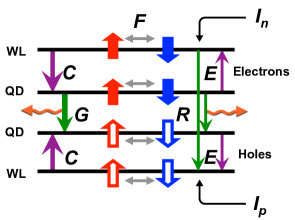
Figure 12: (Color online) Processes in QD spin lasers described by Eqs. (26). QD (WL) represents the level for the quantum dot (wetting layer). The upper two levels are for electrons and the lower levels represent levels for holes. The thick vertical arrows show the carrier spin filled for electrons, empty for holes. The thin arrows depict carrier injection $I$, capture $C$, escape $E$, spin relaxation $F$, and stimulated $G$ and spontaneous $R$ recombination in QDs and QWs (thickness indicates relative rates). The subscripts $n$ and $p$ represent the electron and hole contributions, respectively. Wavy arrows depict photon emission.

An important difference between QW and QD spin laser REs is that only QD spin laser REs have explicit terms for hole occupancies. In QW spin lasers, hole densities can be easily replaced by electron densities as discussed above ($\tau_{sp}\to 0$). However, for QDs, unlike QWs, the ultrafast spin relaxation time for holes ($\tau_{spw},\tau_{spq}\to 0$), does not lift the explicit hole density dependence of QD REs. This makes it more difficult to analytically study QD spin lasers even in the steady state. A generalization of the QD Eqs. (7)-(9) for spin lasers is

$$df_{w\alpha\pm}/dt = I_{\alpha\pm}-C_{\alpha\pm}+\frac{2}{\kappa_{\alpha}}E_{\alpha\pm}-R_{w\pm}\mp F_{w\alpha},$$

$$df_{q\alpha\pm}/dt = \frac{\kappa_{\alpha}}{2}C_{\alpha\pm}-E_{\alpha\pm}-R_{q\pm}-G_{\pm}\mp F_{q\alpha},$$

$$df_{S\mp}/dt = G_{\pm}+\beta R_{q\pm}-f_{S\mp}/\tau_{\mathrm{ph}},$$ (26)

where $\alpha=n,\,p$ denotes electrons and holes, respectively. $I$, $C$, $E$, $G$, and $R$ represent injection, capture, escape, the stimulated and spontaneous emission, respectively, as in unpolarized REs, while $F$ represents spin relaxation. The level scheme of a QD spin laser is shown in Fig. 12. Since the occupancies satisfy $0\leq f_{(w,q)}\leq 1$, the spin-polarized occupancies are defined as $f_{w\alpha\pm}=\bar{n}_{w\alpha\pm}/(N_{w\alpha}/2)$, $f_{q\alpha\pm}=\bar{n}_{w\alpha\pm}/N_{q}$ and $f_{S\pm}=S_{\pm}/N_{q}$, which are different by a factor of 2 from Eqs. (7)-(9). The carrier injection, capture, and escape are $I_{\alpha\pm}=j_{\alpha\pm}(1-f_{w\alpha\pm})$, $C_{\alpha\pm}=f_{w\alpha\pm}(1-f_{q\alpha\pm})/\tau_{c\alpha}$, and $E_{\alpha\pm}=f_{q\alpha\pm}(1-f_{w\alpha\pm})/\tau_{e\alpha}$, where the injection $j_{\alpha\pm}=(1\pm p_{j\alpha})j_{\alpha}$ can be expressed via the corresponding spin polarization $p_{j\alpha}=(j_{\alpha+}-j_{\alpha-})/(j_{\alpha+}+j_{\alpha-})$. The stimulated and spontaneous emission are $G_{\pm}=g(f_{qn\pm}+f_{qp\pm}-1)f_{S\pm}$ and $R_{\eta\pm}=b_{\eta}f_{\eta n\pm}f_{\eta p\pm}$, respectively, where $\eta=w,q$, and $b_{\eta}$ is the recombination rate. The spin relaxation term is $F_{\eta\alpha}=(f_{\eta\alpha+}-f_{\eta\alpha-})/\tau_{s\alpha\eta}$, where $\tau_{s\alpha\eta}$ is the spin relaxation time. In this paper, we assume $\tau_{c\alpha}=\tau_{c}$, $\tau_{e\alpha}=\tau_{e}$, $\tau_{sp\eta}=0$, $\tau_{sn\eta}=\tau_{s}$, $\beta=0$, $j_{\alpha}=j$ and $p_{j\alpha}=P_{J}$.

Appendix B

A linearization of the QW laser REs Eqs. (4) and (5), under a small modulation, leads to the equations for small-signal analysis,Chuang:2009

$$\begin{bmatrix}A_{1}-i\omega&A_{2}\\ -A_{3}&A_{4}-i\omega\end{bmatrix}\left[\begin{array}[]{c}\delta n\\ \delta S\end{array}\right]=\left[\begin{array}[]{c}\delta J\\ 0\end{array}\right],$$ (31)

where the positive matrix elements $A_{1}$, $A_{2}$, $A_{3}$, and $A_{4}$ are defined as

$$A_{1}=2Bn_{0}+\frac{g_{0}}{1+\epsilon S_{0}}S_{0}, A_{2}=\frac{g_{0}(n_{0}-n_{\mathrm{tran}})}{(1+\epsilon S_{0})^{2}},$$

$$A_{3}=\frac{\Gamma g_{0}(n_{0}-n_{\mathrm{tran}})S_{0}}{(1+\epsilon S_{0})}, A_{4}=\frac{1}{\tau_{\mathrm{ph}}}-\frac{\Gamma g_{0}(n_{0}-n_{\mathrm{tran}})}{(1+\epsilon S_{0})^{2}},$$

expressed in terms of the quantities introduced in discussion of Eqs. (4) and (5), as well as their steady-state solutions $n_{0}$ and $S_{0}$ at $J=J_{0}$ . We can obtain the normalized frequency response function as defined in Eq. (15) with relaxation oscillation frequency $\omega_{R}$ and damping factor $\gamma$, given by

$$\omega_{R}^{2}=\frac{g_{0}S_{0}}{\tau_{\mathrm{ph}}(1+\epsilon\,S_{0})}(1+2Bn_{0}\epsilon/g_{0})$$ (33)

and

$$\gamma=2Bn_{0}+K\,[\omega_{R}^{2}/(2\pi)]^{2},$$ (34)

where $K=(\tau_{\mathrm{ph}}+\epsilon/g_{0})/(1+2Bn_{0}\epsilon/g_{0})$ is the so-called more precise definition of $K$ factor without approximations. A widely used approximation above the threshold, $2Bn_{0}\approx 2Bn_{T}$,Chuang:2009 can also be accurately applied for our mapping. On the other hand, the term $2Bn_{0}\epsilon/g_{0}$ in Eq. (33) is often ignored,Chuang:2009 but has to be retained for our purposes of implementing a mapping [Eqs. (B)-(34)] with $\epsilon_{s,d},$ several orders of magnitude greater than the typical compression factors in QW lasers. We therefore use an exact expression for $\omega_{R}$ and $K$ with finite $\epsilon$ (while considering $\beta=0$ limit). The bandwidth $\omega_{\mathrm{3dB}}$ (a function of injection through $\omega_{R}$) is defined as a frequency that reduces the normalized response function to $1/\sqrt{2}$, determined by the equation

$$(\omega_{R}^{2}-\omega_{\mathrm{3dB}}^{2})^{2}+\omega_{\mathrm{3dB}}^{2}\gamma^{2}=2\,\omega_{R}^{4},$$ (35)

which yields Eq. (18) as its the solution. $\omega_{\mathrm{3dB}}$ is a maximum when the denominator of the normalized response function [Eq. (15)] monotonically increases under the condition

$$\omega_{R}^{2}-\gamma^{2}/2=0.$$ (36)

The bandwidth coincides with $\omega_{R}$ [Eq. (18)] when the condition of Eq. (36) is satisfied, which can be written as

$$\omega_{\mathrm{3dB}}^{\mathrm{max}}=\left[2B\,n_{0}+K\left(\frac{\omega_{\mathrm{3dB}}^{\mathrm{max}}}{2\pi}\right)^{2}\right]/\sqrt{2},$$ (37)

and we can find the $K$ factor as a function of the maximum bandwidth. For the dynamic mapping, we substitute for $\omega_{\mathrm{3dB}}^{\mathrm{max}}$ the maximum bandwidth obtained from the QD laser REs. Once the $K$-factor is found, its definition leads us to $\epsilon_{d}$. With the approximations $\omega_{\mathrm{3dB}}^{\mathrm{max}}\gg 2Bn_{0}$ and $2Bn_{0}\epsilon/g_{0}\ll 1$, Eq. (

References

- (1) S. L. Chuang, Physics of Optoelectronic Devices, 2nd ed. (Wiley, New York, 2009).
- (2) M. A. Parker, Physics of Optoelectronics (CRC, New York, 2004).
- (3) L. A. Coldren and S. W. Corzine, Diode Lasers and Photonic Integrated Circuits, (Wiley, New York, 1995).
- (4) W. W. Chow and S. W. Koch, Semiconductor-Laser Fundamentals: Physics of the Gain Materials (Springer, New York, 1999).
- (5) H. Haken, Light, Vol. 2 Laser Light Dynamics (North-Holland, New York, 1985).
- (6) Z. I. Alferov, Rev. Mod. Phys. 73, 767 (2001).
- (7) V. M. Ustinov, A. E. Zhukov, A. Yu. Egorov, and N. A. Maleev, Quantum Dot Lasers (Oxford University Press, New York, 2003).
- (8) D. Bimberg, M. Grundmann, and N. N. Ledentsov, Quanutm Dot Heterostructures (Wiley, New York, 1999).
- (9) A. Das, J. Heo, M. Jankowski, W. Guo, L. Zhang, H. Deng, and P. Bhattacharya, Phys. Rev. Lett. 107, 066405 (2011).
- (10) J. Rudolph, D. Hägele, H. M. Gibbs, G. Khitrova, and M. Oestreich, Appl. Phys. Lett. 82, 4516 (2003).
- (11) J. Rudolph, S. Döhrmann, D. Hägele, M. Oestreich, and W. Stolz, Appl. Phys. Lett. 87, 241117 (2005).
- (12) M. Holub, J. Shin, and P. Bhattacharya, Phys. Rev. Lett. 98, 146603 (2007).
- (13) V. Degiorgio and. M. O. Scully, Phys. Rev. A 2, 1170 (1970).
- (14) V. Degiorgio, Phys. Today 29(10), 42 (1976).
- (15) L. V. Asryan and R. A. Suris, in Selected Topics in Electronics and Systems, edited by E. Borovitskaya and M. E. Shur, Vol. 25 (World Scientific, Singapore, 2002).
- (16) I. Sellers, H. Liu, K. Groom, D. Childs, D. Robbins, T. Badcock, M. Hopkinson, D. Mowbray, and M. Skolnick, Electron. Lett. 40, 1412 (2004).
- (17) C. Gøthgen, R. Oszwałdowski, A. Petrou, and I. Žutić, Appl. Phys. Lett. 93, 042513 (2008).
- (18) R. Oszwałdowski, C. Gøthgen, and I. Žutić, Phys. Rev. B 82, 085316 (2010).
- (19) J. Lee, W. Falls, R. Oszwałdowski, and I. Žutić, Spin modulation in lasers, Appl. Phys. Lett. 97, 041116 (2010).
- (20) D. Basu, D. Saha, C. C. Wu, M. Holub, Z. Mi and P. Bhattacharya, Appl. Phys. Lett. 92, 091119 (2008).
- (21) D. Basu, D. Saha and P. Bhattacharya, Phys. Rev. Lett. 102, 093904 (2009).
- (22) D. Saha, D. Basu, and P. Bhattacharya, Phys. Rev. B 82, 205309 (2010).
- (23) Optical Orientation, edited by F. Meier and B. P. Zakharchenya (North-Holland, New York, 1984).
- (24) I. Žutić, J. Fabian and S. Das Sarma, Rev. Mod. Phys. 76, 323 (2004).
- (25) I. Žutić, J. Fabian, and S. Das Sarma, Phys. Rev. B 64, 121201(R) (2001).
- (26) B. M. Vulović, I. Ovchinnikov, and K. L. Wang, J. Appl. Phys. 109, 063916 (2011).
- (27) S. Iba, S. Koh, K. Ikeda, and H. Kawaguchi, Appl. Phys. Lett. 98, 081113 (2011).
- (28) H. Dery and G. Eisenstein, IEEE J. Quantum Electron. 41, 26 (2005)
- (29) A. Fiore and A. Markus, IEEE J. Quantum Electron. 43, 287 (2007).
- (30) H.D. Summers, and P. Rees, J. Appl. Phys. 101, 073106 (2007).
- (31) M. W. Taylor, E. Harbord, P. Spencer, E. Clarke, G. Slavcheva, and R. Murray, Appl. Phys. Lett. 97, 171907 (2010).
- (32) We mostly consider while the results for can be deduced easily.
- (33) I. Vurgaftman, M. Holub, B. T. Jonker, and J. R. Mayer, Appl. Phys. Lett. 93, 031102 (2008).
- (34) M. Oestreich, J. Rudolph, R. Winkler, and D. Hägele, Superlattices Microstruct. 37, 306 (2005).
- (35) M. Holub and B. T. Jonker, Phys. Rev. B 83, 125309 (2011).
- (36) M. San Miguel, Q. Feng, and J. V. Moloney, Phys. Rev. A 52, 1728 (1995).
- (37) A. Dyson and M. J. Adams, J. Opt. B: Quantum Semiclass. Opt. 5, 222 (2003).
- (38) M. J. Adams and D. Alexandropoulos, IEEE J. Quantum Electron. 45, 744 (2009).
- (39) R. Al-Seyab, D. Alexandropoulos, I. D. Henning, and M. H. Adams, IEEE Photonics J. 3, 799 (2011).
- (40) N. C. Gerhardt, M. Y. Li, H. Jähme, H. Höpfner, T. Ackemann, and M. R. Hofmann, Appl. Phys. Lett. 99, 151107 (2011).
- (41) M. Li, H. Jähme, H. Soldat, N. C. Gerhardt, M. R. Hofmann, and T. Ackemann, Appl. Phys. Lett. 97, 191114 (2010).
- (42) H. Dery and G. Eisenstein, IEEE J. of Quantum Electron. 40, 1398 (2004).
- (43) J. Huang and L. W. Casperson, Opt. Quant. Electron. 25, 369 (1993).
- (44) I. Žutić, J. Fabian, and S. C. Erwin, Phys. Rev. Lett. 97, 026602 (2006).
- (45) S. F. Yu, Analysis and Design of Vertical Cavity Surface Emitting Lasers (Wiley, New York, 2003).
- (46) A. Yariv, Optical Electronics in Modern Communications, 5th ed. (Oxford University Press, New York, 1997).
- (47) Y. B. Ezra, B. I. Lembrikov and M. Hardim, IEEE J. Quantum Electron. 45, 34 (2009).
- (48) T. Erneus, E. A. Viktorov, and P. Mandel, Phys. Rev. A 76, 023819 (2007).
- (49) and correspond to 133 and 420 ps in terms of recombination time assuming linear recombinations giving the same threshold.
- (50) Index represents dynamic mapping, refer to Sec. IV.
- (51) G. Fowles and G. Cassiday, Analytical Mechanics, 7th ed. (Brooks/Cole, Belmont, 2005).
- (52) Strictly speaking, the term “relaxation oscillation frequency” is not completely accurate although it is frequently used in the literature with the underlying assumption . In analogy to the classical oscillator, here corresponds to the “intrinsic” or “natural” frequency as shown in Ref. Fowles:2005, .
- (53) L. V. Asryan and R. A. Suris, Appl. Phys. Lett. 96, 221112 (2010).
- (54) R. Nagarajan, M. Ishikawa, T. Fukushima, R. S. Geels, and J. E. Bowers, IEEE J. Quantum Electron. 28, 1990 (1992).
- (55) M. Sugawara, K. Mukai, and H. Shoji, Appl. Phys. Lett. 71, 2791 (1997).
- (56) B. Ohnesorge, M. Albrecht, J. Oshinowo, and A. Forchel, Phys. Rev. B 54, 53 (1996).
- (57) R. Heitz, M. Veit, N. N. Ledentsov, A. Hoffmann, D. Bimberg, V. M. Ustinov, P. S. Kop’ev, and Zh. I. Alferov, Phys. Rev. B 56, 10435 (1997).
- (58) T. Müller, F. F. Schrey, G. Strasser, and K. Unterrainer, Appl. Phys. Lett. 83, 3572 (2003).
- (59) M. Ishida, F. F. Schrey, G. Strasser, and K. Unterrainer, Appl. Phys. Lett. 85, 4145 (2004).
- (60) S. Hövel, N. C. Gerhardt, C. Brenner, M. R. Hofmann, F.-Y. Lo, D. Reuter, A. D. Wieck, E. Schuster and W. Keune, Physica Status Solid (a) 204, 500 (2007).
- (61) A. Bischoff, N. C Gerhardt, M. R. Hofmann, T. Ackemann, A. Kroner, and R. Michalzik, Appl. Phys. Lett. 92, 041118 (2008).
- (62) H. Ando, T. Sogawa, and H. Gotoh, Appl. Phys. Lett. 73, 566 (1998).
- (63) S. Hallstein, J. D. Berger, M. Hilpert, H. C. Schneider, W. W. Rühle, F. Jahnke, S. W. Koch, H. M. Gibbs, G. Khitrova, M. Oestreich, Phys. Rev. B 56, R7076 (1997).
- (64) H. Soldat, M. Li, N. C. Gerhardt, M. R. Hofmann, A. Ludwig, A. Ebbing, D. Reuter, A. D. Wieck, F. Stromberg, W. Keune, and H. Wende, Appl. Phys. Lett. 99, 051102 (2011).
- (65) E. D. Fraser, S. Hegde, L. Schweidenback, A. H. Russ, A. Petrou, H. Luo, and G. Kioseoglou, Appl. Phys. Lett. 97, 041103 (2010).
- (66) J. Fabian, A. Matos-Abiague, C. Ertler, P. Stano, and I. Žutić, Acta Phys. Slov. 57, 565 (2007).
- (67) H. Fujino, S. Koh, S. Iba, T. Fujimoto, and H. Kawaguchi, Appl. Phys. Lett. 94, 131108 (2009).
- (68) K. Ikeda, T. Fujimoto, H. Fujino, T. Katayama, S. Koh, and H. Kawaguchi, IEEE Photon. Technol. Lett. 21, 1350 (2009).
- (69) S. Iba, S. Koh, and H. Kawaguchi, Appl. Phys. Lett. 97, 202102 (2010).
- (70) D. Banerjee, R. Adari, M. Murthy, P. Suggisetti, S. Ganguly, and D. Saha, J. Appl. Phys. 109, 07C317 (2011).
- (71) J. D. Bull, N. A. F. Jaeger, H. Kato, M. Fairburn, A. Reid, and P. Ghanipour, in Photonic North 2004: Optical Components and Devices, edited by J. C. Armitage, S. Fafard, R. A. Lessard, and G. A. Lampropoulos, eds., [Proc. SPIE 5577, 133 (2004)].
- (72) A. T. Hanbicki, O. M. van’t Erve, R. Magno, G. Kioseoglou, C. H. Li, B. T. Jonker, G. Itskos, R. Mallory, and A. Petrou, Appl. Phys. Lett. 82, 4092 (2003).
- (73) G. Salis, R. Wang, X. Jiang, R. M. Shelby, S. S. P. Parkin, S. R. Bank, and J. S. Harris, Appl. Phys. Lett. 87, 262503 (2005).
- (74) T. J. Zega, A. T. Hanbicki, S. C. Erwin, I. Žutić, G. Kioseoglou, C. H. Li, B. T. Jonker, and R. M. Stroud, Phys. Rev. Lett. 96, 196101 (2006).
- (75) S. A. Crooker, E. S. Garlid, A. N. Chantis, D. L. Smith, K. S. M. Redd, Q. O. Hu, T. Kondo, and C. J. Palmstrøm, and P. A. Crowell, Phys. Rev. B 80, 041305 (R) (2009).
- (76) P. Li and H. Dery, Appl. Phys. Lett. 94, 192108 (2009).
- (77) This is not essential but simplifies our analytical results.
- (78) H. Dery, J. Song, P. Li, and I. Žutić, Appl. Phys. Lett. 99, 082502 (2011).
- (79) S. Fathpour, Z. Mi, and P. Bhattacharya, J. Phys. D: Appl. Phys. 38, 2103 (2005).
- (80) V. I. Klimov, S. A. Ivanov, J. Nanda, M. Achermann, I. Bezel, J. A. McGuire, and A. Piryatinski, Nature (London) 447, 441 (2007).
- (81) G. D. Scholes, Adv. Funct. Mater. 18, 1157 (2008).
- (82) R. Beaulac, P. I. Archer, S. T. Ochsenbein, and D. R. Gamelin, Adv. Funct. Mater. 18, 3873 (2008).
- (83) N. P. Stern, M. Poggio, M. H. Bartl, E. L. Hu, G. D. Stucky, and D. D. Awschalom, Phys. Rev. B 72, 161303 (R) (2005).
- (84) O. R. Qasaimeh, J. Lightwave Technol., 27, 2530 (2009).