Quasisymmetry and Rectifiability of Quasispheres

Abstract.

We obtain Dini conditions that guarantee that an asymptotically conformal quasisphere is rectifiable. In particular, we show that for any $\epsilon>0$ integrability of $({\rm ess}\sup_{1-t<|x|<1+t}K_{f}(x)-1)^{2-\epsilon}dt/t$ implies that the image of the unit sphere under a global quasiconformal homeomorphism $f$ is rectifiable. We also establish estimates for the weak quasisymmetry constant of a global $K$-quasiconformal map in neighborhoods with maximal dilatation close to 1.

1. Introduction

A quasisphere $f(S^{n-1})$ is the image of the unit sphere $S^{n-1}\subset\mathbb{R}^{n}$ under a global quasiconformal mapping $f:\mathbb{R}^{n}\rightarrow\mathbb{R}^{n}$. In the plane, a quasisphere is a quasicircle. (Look below for the definition of a quasiconformal map.) It is well known that the Hausdorff dimension of a quasisphere can exceed $n-1$. When $n=2$, for example, the von Koch snowflake is a quasicircle with dimension $\log 4/\log 3>1$. In fact, every quasicircle is bi-Lipschitz equivalent to a snowflake-like curve (see Rohde [16]). On the other hand, the Hausdorff dimension of a quasicircle cannot be too large: Smirnov [18] proved Astala’s conjecture that every $k$-quasicircle ($0\leq k<1$) has dimension at most $1+k^{2}$. This result was further enhanced by Prause, Tolsa and Uriarte-Tuero [13] who showed that $k$-quasicircles have finite $(1+k^{2})$-dimensional Hausdorff measure. The picture in higher dimensions is not as complete. A few detailed examples of quasispheres with dimension greater than $n-1$ ($n\geq 3$) have been described by David and Toro [4] and Meyer [10], [11]. Mattila and Vuorinen [9] have also demonstrated how the maximal dilatation (see (1.1)) of a quasiconformal map $f$ controls the geometry and size of the quasisphere $f(S^{n-1})$. More specifically, they showed that if $f$ is $K$-quasiconformal with $K$ near 1, then $f(S^{n-1})$ satisfies the linear approximation property (see [9]) and this property bounds the dimension of $f(S^{n-1})$. Mattila and Vuorinen’s proof that quasispheres are locally uniformly approximable by hyperplanes was recently streamlined by Prause [12], using the quasisymmetry of $f$. This idea from [12] will play an important role in our analysis below.

In the current article, we seek optimal conditions on $f$ that ensure $f(S^{n-1})$ has finite $(n-1)$-dimensional Hausdorff measure $\mathcal{H}^{n-1}$. We obtain two such conditions, one expressed in terms of the dilatation of $f$ (Theorem 1.1) and one expressed in terms of the quasisymmetry of $f$ (Theorem 1.2), and both have sharp exponent. This problem was previously studied in the case $n=2$ by Anderson, Becker and Lesley [2] and in all dimensions by Mattila and Vuorinen [9]. To state these results and the main results of this paper, we require some additional notation.

Let $1\leq K<\infty$. A mapping $f:\Omega\rightarrow\mathbb{R}^{n}$ from a domain $\Omega\subset\mathbb{R}^{n}$ ($n\geq 2$) is said to be $K$-quasiconformal (analytic definition) if $f\in W^{1,n}_{\mathrm{loc}}(\Omega)$, if $f$ is a homeomorphism onto its image, and if the maximal dilatation $K_{f}(\Omega)$ is bounded by $K$:

(1.1) $$K_{f}(\Omega)=\max\left\{\mathop{\mathrm{missing}}{ess\,sup}_{x\in\Omega}\frac{\|f^{\prime}(x)\|^{n}}{|Jf(x)|},\mathop{\mathrm{missing}}{ess\,sup}_{x\in\Omega}\frac{|Jf(x)|}{\ell(f^{\prime}(x))^{n}}\right\}\leq K.$$

Here we let $f^{\prime}$ and $Jf$ denote the Jacobian matrix and Jacobian determinant of $f$, respectively. Also $\|\cdot\|$ denotes the operator norm and $\ell(f^{\prime}(x))=\min_{\|v\|=1}|f^{\prime}(x)v|$. For background on quasiconformal maps in higher dimensions, we refer the reader to Väisälä [20] and Heinonen [7]. For $t>0$, set $A_{t}=\{x\in\mathbb{R}^{n}:1-t<|x|<1+t\}$, the annular neighborhood of $S^{n-1}$ of size $t$. We say that a quasisphere $f(S^{n-1})$ is asymptotically conformal if $K_{f}(A_{t})\rightarrow 1$ as $t\rightarrow 0$. It will be convenient to also introduce the notation

(1.2) $$\widetilde{K}_{f}(\Omega)=K_{f}(\Omega)-1.$$

Notice that $K_{f}(A_{t})\rightarrow 1$ as $t\rightarrow 0$ if and only if $\widetilde{K}_{f}(A_{t})\rightarrow 0$ as $t\rightarrow 0$.

Every asymptotically conformal quasisphere $f(S^{n-1})$ has Hausdorff dimension $n-1$; see Remark 2.8. This is the best that we can do in general, because there are snowflake-like curves $\Gamma=f(S^{1})$ such that $\widetilde{K}_{f}(A_{t})\rightarrow 0$ as $t\rightarrow 0$ but $\mathcal{H}^{1}(\Gamma)=\infty$. The main obstruction to finite Hausdorff measure is that $\widetilde{K}_{f}(A_{t})$ could converge to $0$ very slowly as $t\rightarrow 0$. Conversely, one expects that a good rate of convergence should guarantee that $\mathcal{H}^{n-1}(f(S^{n-1}))<\infty$. One would like to determine the threshold for a “good rate”. In [2] Anderson, Becker and Lesley proved that (in our notation) if $f:\mathbb{R}^{2}\rightarrow\mathbb{R}^{2}$ is quasiconformal and $f|_{B(0,1)}$ is conformal, then

(1.3) $$\int_{0}^{1}\left(\widetilde{K}_{f}(A_{t})\right)^{2}\frac{dt}{t}<\infty\quad\Longrightarrow\quad\mathcal{H}^{1}(f(S^{1}))<\infty.$$

It is also known that the exponent $2$ in the Dini condition (1.3) cannot be weakened to $2+\epsilon$ for any $\epsilon>0$ (see [2]). In higher dimensions, Mattila and Vuorinen [9] proved that (in our notation)

(1.4) $$\int_{0}^{1}\widetilde{K}_{f}(A_{t})\frac{dt}{t}<\infty\quad\Longrightarrow\quad f|_{S^{n-1}}\text{ is Lipschitz.}$$

Hence, by a standard property of Lipschitz maps, the Dini condition in (1.4) also implies that the quasisphere $f(S^{n-1})$ is $(n-1)$-rectifiable and $\mathcal{H}^{n-1}(f(S^{n-1}))<\infty$. In fact, something more is true: the Dini condition $(\ref{MVeq})$ implies that $f(S^{n-1})$ is a $C^{1}$ submanifold of $\mathbb{R}^{n}$ (see Chapter 7, §4 in Reshetnyak [15]). For conditions weaker than (1.4) (but also with “exponent 1”) that imply $f|_{S^{n-1}}$ is Lipschitz, see Bishop, Gutlyanskiĭ, Martio and Vuorinen [3] and Gutlyanskiĭ and Golberg [6]. Notice that the Dini condition (1.4) is stronger (harder to satisfy) than the Dini condition (1.3). The main result of this paper is that a Dini condition with exponent 2 ensures that $\mathcal{H}^{n-1}(f(S^{n-1}))<\infty$ in dimensions $n\geq 3$, and moreover guarantees the existence of local bi-Lipschitz parameterizations.

Theorem 1.1.

If $f:\mathbb{R}^{n}\rightarrow\mathbb{R}^{n}$ is quasiconformal and

(1.5) $$\int_{0}^{1}\left(\widetilde{K}_{f}(A_{t})\log\frac{1}{\widetilde{K}_{f}(A_{t})}\right)^{2}\frac{dt}{t}<\infty,$$

then the quasisphere $f(S^{n-1})$ admits local $(1+\delta)$-bi-Lipschitz parameterizations, for every $\delta>0$. Thus $f(S^{n-1})$ is $(n-1)$-rectifiable and $\mathcal{H}^{n-1}(f(S^{n-1}))<\infty$.

The main difference between Mattila and Vuorinen’s theorem and Theorem 1.1 is that the former is a statement about the regularity of $f|_{S^{n-1}}$, while the latter is a statement about the regularity of $f(S^{n-1})$. The logarithmic term in (1.5) is an artifact from the proof of Theorem 1.1, which occurs when we use the maximal dilatation of the map $f$ to control the weak quasisymmetry constant of $f$ (see (1.9)). We do not know whether this term can be removed, and leave this open for future investigation. Nevertheless, Theorem 1.1 has the following immediate consequence. If $f:\mathbb{R}^{n}\rightarrow\mathbb{R}^{n}$ is quasiconformal and

(1.6) $$\int_{0}^{1}\left(\widetilde{K}_{f}(A_{t})\right)^{2-\epsilon}\frac{dt}{t}<\infty\quad\text{for some }\epsilon>0,$$

then $f$ satisfies (1.5), and in particular, the quasisphere $f(S^{n-1})$ satisfies the same conclusions as in Theorem 1.1. The exponent 2 in Theorem 1.1 is the best possible, i.e. 2 cannot be replaced with $2+\epsilon$ for any $\epsilon>0$. For example, the construction in David and Toro [4] (with the parameters $Z=\mathbb{R}^{n-1}$ and $\epsilon_{j}=1/j$) can be used to produce a quasiconformal map $f:\mathbb{R}^{n}\rightarrow\mathbb{R}^{n}$ such that

(1.7) $$\int_{0}^{1}\left(\widetilde{K}_{f}(\{x\in\mathbb{R}^{n}:|x_{n}|<t\})\right)^{2+\epsilon}\frac{dt}{t}<\infty\quad\text{for all }\epsilon>0,$$

but for which the associated “quasiplane” $f(\mathbb{R}^{n-1})$ is not $(n-1)$-rectifiable and has locally infinite $\mathcal{H}^{n-1}$ measure.

To prove Theorem 1.1 we first prove a version where the maximal dilatation in the Dini condition is replaced with the weak quasisymmetry constant. Recall that a topological embedding $f:\Omega\rightarrow\mathbb{R}^{n}$ is called quasisymmetric if there exists a homeomorphism $\eta:[0,\infty)\rightarrow[0,\infty)$ such that

(1.8) $$|x-y|\leq t|x-z|\Rightarrow|f(x)-f(y)|\leq\eta(t)|f(x)-f(z)|\quad\text{for all }x,y,z\in\Omega.$$

Every $K$-quasiconformal map $f:\mathbb{R}^{n}\rightarrow\mathbb{R}^{n}$ is quasisymmetric for some gauge $\eta_{n,K}$ determined by $n$ and $K$; e.g., see Heinonen [7]. Below we only use (1.8) with $t=1$. This leads to the concept of weak quasisymmetry.

Let $1\leq H<\infty$. An embedding $f:\Omega\rightarrow\mathbb{R}^{n}$ is weakly $H$-quasisymmetric if

(1.9) $$H_{f}(\Omega)=\sup\left\{\frac{|f(x)-f(y)|}{|f(x)-f(z)|}:x,y,z\in\Omega\text{ and }\frac{|x-y|}{|x-z|}\leq 1\right\}\leq H.$$

We call $H_{f}(\Omega)$ the weak quasisymmetry constant of $f$ on $\Omega$. Also set

(1.10) $$\widetilde{H}_{f}(\Omega)=H_{f}(\Omega)-1.$$

We will establish the following theorem in §2.

Theorem 1.2.

If $f:\mathbb{R}^{n}\rightarrow\mathbb{R}^{n}$ is quasiconformal and

(1.11) $$\int_{0}^{1}\sup_{z\in S^{n-1}}\left(\widetilde{H}_{f}(B(z,t))\right)^{2}\frac{dt}{t}<\infty,$$

then the quasisphere $f(S^{n-1})$ admits local $(1+\delta)$-bi-Lipschitz parameterizations, for every $\delta>0$. Thus $f(S^{n-1})$ is $(n-1)$-rectifiable and $\mathcal{H}^{n-1}(f(S^{n-1}))<\infty$.

The proof of Theorem 1.2 is based on the connection between the quasisymmetry of $f$ near $S^{n-1}$ and the flatness of the set $f(S^{n-1})$ (first described in Prause [12]), and a criterion for existence of local bi-Lipschitz parameterizations from Toro [19].

The maximal dilatation and weak quasisymmetry constant are related as follows. For any $\Omega\subset\mathbb{R}^{n}$ and quasiconformal map $f:\Omega\rightarrow\mathbb{R}^{n}$,

(1.12) $$K_{f}(\Omega)\leq\mathop{\mathrm{missing}}{ess\,sup}_{x\in\Omega}\frac{\|f^{\prime}(x)\|^{n-1}}{\ell(f^{\prime}(x))^{n-1}}\leq H_{f}(\Omega)^{n-1}.$$

In particular, $\widetilde{K}_{f}(\Omega)\leq C\widetilde{H}_{f}(\Omega)$ when $H_{f}(\Omega)$ is close to 1. Hence

(1.13) $$\sup_{z\in S^{n-1}}\widetilde{H}_{f}(B(z,t))\rightarrow 0\ \text{ as }\ t\rightarrow 0\quad\Longrightarrow\quad\widetilde{K}_{f}(A_{t})\rightarrow 0\ \text{ as }\ t\rightarrow 0.$$

The question of whether or not the implication in (1.13) can be reversed is delicate. When $n=2$ and $f$ is a quasiconformal map of the plane, $H_{f}(\mathbb{R}^{2})\leq\exp(C\widetilde{K}_{f}(\mathbb{R}^{2}))$ (see Theorem 10.33 in [1]). Therefore,

(1.14) $$\widetilde{H}_{f}(\mathbb{R}^{2})\leq C\widetilde{K}_{f}(\mathbb{R}^{2})\quad\text{when }\widetilde{K}_{f}(\mathbb{R}^{2})\ll 1.$$

When $n\geq 3$ and $f$ is a quasiconformal map of space (see Theorem 2.7 in [12]),

(1.15) $$\widetilde{H}_{f}(\mathbb{R}^{n})\leq C\widetilde{K}_{f}(\mathbb{R}^{n})\log\left(\frac{1}{\widetilde{K}_{f}(\mathbb{R}^{n})}\right)\quad\text{when }\widetilde{K}_{f}(\mathbb{R}^{n})\ll 1.$$

In order to derive Theorem 1.1 from Theorem 1.2, we need (1.15) with $B(z,t)$ in place of $\mathbb{R}^{n}$, uniformly for all $z\in S^{n-1}$. Unfortunately, to the best of our knowledge such an estimate does not appear in the literature. Thus, in §3, we show how to localize (1.15). We establish an upper bound on the weak quasisymmetry constant of a global quasiconformal map in neighborhoods with maximal dilatation near 1 (see Theorem 3.1). As a consequence, it follows that (see Corollary 3.2)

(1.16) $$\widetilde{K}_{f}(A_{t})\rightarrow 0\ \text{ as }\ t\rightarrow 0\quad\Longrightarrow\quad\sup_{z\in S^{n-1}}\widetilde{H}_{f}(B(z,t))\rightarrow 0\ \text{ as }\ t\rightarrow 0.$$

Thus, combining (1.13) and (1.16), we conclude that a quasisphere $f(S^{n-1})$ is asymptotically conformal if and only if $\widetilde{H}_{f}(B(z,t))\rightarrow 0$ as $t\rightarrow 0$, uniformly across $z\in S^{n-1}$.

The remainder of this paper is divided into two sections, each aimed at the proof of a Dini condition for rectifiability of $f(S^{n-1})$. First we prove Theorem 1.2 in §2. Then we prove Theorem 1.1 in §3.

2. Quasisymmetry and Local Flatness

The goal of this section is to prove Theorem 1.2. Following an idea of Prause [12], we show that the weak quasisymmetry of $f|_{A_{t}}$ controls the local flatness of $f(S^{n-1})$ at scales depending on $t$. We then invoke a theorem on the existence of local bi-Lipschitz parameterizations from Toro [19].

Let $\Sigma\subset\mathbb{R}^{n}$ $(n\geq 2$) be a closed set. The local flatness $\theta_{\Sigma}(x,r)$ of $\Sigma$ near $x\in\Sigma$ at scale $r>0$ is defined by

(2.1) $$\theta_{\Sigma}(x,r)=\frac{1}{r}\min_{L\in G(n,n-1)}\mathop{\mathrm{missing}}{HD}[\Sigma\cap B(x,r),(x+L)\cap B(x,r)],$$

where $G(n,n-1)$ denotes the collection of $(n-1)$-dimensional subspaces of $\mathbb{R}^{n}$ (i.e. hyperplanes through the origin) and $\mathop{\mathrm{missing}}{HD}[A,B]$ denotes the Hausdorff distance between nonempty, bounded subsets $A,B\subset\mathbb{R}^{n}$,

(2.2) $$\mathop{\mathrm{missing}}{HD}[A,B]=\max\left\{\sup_{x\in A}\,\mathop{\mathrm{missing}}{dist}(x,B),\ \sup_{y\in B}\,\mathop{\mathrm{missing}}{dist}(y,A)\right\}.$$

Thus local flatness is a gauge of how well a set can be approximated by a hyperplane. Notice that $\theta_{\Sigma}(x,r)$ measures the distance of points in the set to a plane and the distance of points in a plane to the set. (By comparison the Jones $\beta$-numbers [8] and Mattila and Vuorinen’s linear approximation property [9] only measure the distance of points in the set to a plane.) Because $\theta_{\Sigma}(x,r)\leq 1$ for every closed set $\Sigma$, every location $x\in\Sigma$ and every scale $r>0$, this quantity only carries information when $\theta_{\Sigma}(x,r)$ is small.

Sets which are uniformly close to a hyperplane at all locations and scales first appeared in Reifenberg’s solution of Plateau’s problem in arbitrary codimension [14]. A closed set $\Sigma\subset\mathbb{R}^{n}$ is called $(\delta,R)$-Reifenberg flat provided that $\theta_{\Sigma}(x,r)\leq\delta$ for all $x\in\Sigma$ and $0<r\leq R$. Moreover, $\Sigma$ is said to be Reifenberg flat with vanishing constant if for every $\delta>0$ there exists a scale $R_{\delta}>0$ such that $\Sigma$ is $(\delta,R_{\delta})$-Reifenberg flat. We now record a rectifiability criterion for locally flat sets, which we need below for the proof of Theorem 1.2. For further information about flat sets and parameterizations, see the recent investigation by David and Toro [5].

Theorem 2.1 (Toro [19]).

Let $n\geq 2$. There exists constants $\delta_{0}>0$, $\epsilon_{0}>0$ and $C>1$ depending only on $n$ with the following property. Assume that $0<\delta\leq\delta_{0}$, $0<\epsilon\leq\epsilon_{0}$, and $\Sigma\subset\mathbb{R}^{n}$ is a $(\delta,R)$-Reifenberg flat set. If $x_{0}\in\Sigma$, $0<r\leq R$, and

(2.3) $$\int_{0}^{r}\sup_{x\in\Sigma\cap B(x_{0},r)}\left(\theta_{\Sigma}(x,t)\right)^{2}\frac{dt}{t}<\epsilon^{2}$$

then there exists a bi-Lipschitz homeomorphism $\tau:\Omega\rightarrow\Sigma\cap B(x,r/64)$ where $\Omega$ is a domain in $\mathbb{R}^{n-1}$; moreover, $\tau$ and $\tau^{-1}$ have Lipschitz constants at most $1+C(\delta+\epsilon)$.

Corollary 2.2.

If $\Sigma\subset\mathbb{R}^{n}$ is Reifenberg flat with vanishing constant and

(2.4) $$\int_{0}^{t_{0}}\sup_{x\in\Sigma}\left(\theta_{\Sigma}(x,t)\right)^{2}\frac{dt}{t}<\infty\quad\text{for some }t_{0}>0,$$

then $\Sigma$ admits local $(1+\delta)$-bi-Lipschitz parameterizations, for every $\delta>0$.

The following lemma is based on an observation by Prause [12], who showed that quasisymmetry bounds the Jones $\beta$-numbers of $f(L)$, where $f$ is quasiconformal and $L$ is a hyperplane. Here we obtain a slightly stronger statement, because we bound the “two-sided” Hausdorff distance between a set and a hyperplane.

Lemma 2.3.

Let $U\subset\mathbb{R}^{n}$ be an open set which contains the closed ball $\overline{B(0,1)}$. Assume that $f:U\rightarrow\mathbb{R}^{n}$ is weakly $H$-quasisymmetric with

(2.5) $$H=1+\epsilon,\quad 0\leq\epsilon\leq 1/20$$

and

(2.6) $$f(\pm e_{1})=\pm e_{1}.$$

If $L=e_{1}^{\perp}$ denotes the hyperplane through the origin, orthogonal to the direction $e_{1}$, then $f(B(0,1))\supset B(f(0),5/6)$ and $\theta_{f(L)}(f(0),1/2)\leq 20\epsilon$.

Proof.

Assume that $U\subset\mathbb{R}^{n}$ is an open set containing the closed ball $\overline{B_{1}}$, where $B_{1}=B(0,1)$. Moreover, assume that $f:U\rightarrow\mathbb{R}^{n}$ is a weakly $H$-quasisymmetric map satisfying (2.5) and (2.6). Let $e_{1}=(1,0,\dots,0)$ and let $L=e_{1}^{\perp}$ denote the $(n-1)$-dimensional plane through the origin that is orthogonal to the direction $e_{1}$. By the polarization identity, for any $y\in\mathbb{R}^{n}$,

(2.7) $$\mathop{\mathrm{missing}}{dist}(y,L)=|\langle y,e_{1}\rangle|=\frac{1}{4}\left||y-e_{1}|^{2}-|y+e_{1}|^{2}\right|.$$

Let $x\in L\cap B_{1}$. Since $|x-e_{1}|=|x+e_{1}|$ and $f(\pm e_{1})=\pm e_{1}$, by weak quasisymmetry,

(2.8) $$\frac{1}{1+\epsilon}\leq\frac{|f(x)-e_{1}|}{|f(x)+e_{1}|}\leq 1+\epsilon.$$

Combining (2.7) and (2.8),

(2.9) $$\mathop{\mathrm{missing}}{dist}(f(x),L)\leq\frac{1}{4}\left((1+\epsilon)^{2}-1\right)\max\{|f(x)\pm e_{1}|^{2}\}.$$

On the other hand, since $|x\pm e_{1}|\leq 2=|\pm e_{1}-(\mp e_{1})|$ for every $x\in B_{1}$, the weak quasisymmetry of $f$ yields

(2.10) $$|f(x)\pm e_{1}|\leq 2(1+\epsilon).$$

Thus, from (2.5), (2.9) and (2.10), we conclude

(2.11) $$\mathop{\mathrm{missing}}{dist}(f(x),L)\leq\left((1+\epsilon)^{2}-1\right)(1+\epsilon)^{2}=\epsilon(2+\epsilon)(1+\epsilon)^{2}\leq 2.5\epsilon.$$

Since the hyperplane $f(0)+L=\langle f(0),e_{1}\rangle e_{1}+L=(\pm\mathop{\mathrm{missing}}{dist}(f(0),L))e_{1}+L$, it follows that

(2.12) $$\mathop{\mathrm{missing}}{dist}(f(x),f(0)+L)\leq 5\epsilon\quad\text{for all }x\in L\cap B_{1}.$$

So far we have bounded the distance of points in the set $f(L\cap B_{1})$ to the hyperplane $f(0)+L$. To estimate the local flatness of $f(L)$ near $f(0)$, we also need to bound the distance of points in $f(0)+L$ to the set $f(L)$.

First we claim that $f(B_{1})\supset B(f(0),5/6)$. To verify this, suppose that $z\in\mathbb{R}^{n}$, $|z|=1$. On one hand, by weak quasisymmetry, (2.5) and (2.6),

(2.13) $$|f(z)-f(0)|\geq\frac{1}{1+\epsilon}|f(e_{1})-f(0)|\geq\frac{20}{21}|e_{1}-f(0)|.$$

On the other hand, pick $w\in L$ such that $|f(0)-w|=\mathop{\mathrm{missing}}{dist}(f(0),L)$. Then (2.5), (2.11) and the triangle inequality yield

(2.14) $$|e_{1}-f(0)|\geq|e_{1}-w|-|f(0)-w|\geq 1-2.5\epsilon\geq 7/8$$

Together (2.13) and (2.14) imply $|f(z)-f(0)|\geq 5/6$. Because $|f(z)-f(0)|\geq 5/6$ for all $|z|=1$ and $f$ is homeomorphism, we conclude that $f(B_{1})\supset B(f(0),5/6)$. Hence, by (2.12), $f(L)\cap B(f(0),5/6)$ is contained in a $5\epsilon$-neighborhood of $f(0)+L$.

Next we consider the sets $S^{\pm}=\{x\in B(f(0),5/6):\langle x-f(0),\pm e_{1}\rangle>5\epsilon\}$. Because the hyperplane $L$ divides $B_{1}$ into two connected components and the map $f$ is a homeomorphism, $f(L)$ divides $f(B_{1})$ into two connected components. Hence, in view of (2.12), we know that $S^{+}$ and $S^{-}$ are contained in different connected components of $B(f(0),5/6)\setminus f(L)$. In particular, every line segment from $\partial S^{+}$ to $\partial S^{-}$ intersects $f(L)$. If $v\in B(f(0),1/2)\cap(f(0)+L)$, then $v\pm 5\epsilon e_{1}\in B(f(0),5/6)$ (since $(1/2)^{2}+(5\epsilon)^{2}<5/6$). Thus the line segment $\ell_{v}$ with endpoints $v\pm 5\epsilon e_{1}$ in $\partial S^{\pm}$ necessarily intersects $f(L)$. Since $v$ is the center of $\ell_{v}$, it follows that

(2.15) $$\mathop{\mathrm{missing}}{dist}(v,f(L))\leq 5\epsilon\quad\text{ for all }v\in B(f(0),1/2))\cap(f(0)+L).$$

Moreover, if $v\in B(f(0),1/2-5\epsilon)\cap(f(0)+L)$, then $\ell_{v}\subset B(f(0),1/2)$ and the upper bound in (2.15) remains valid with $\mathop{\mathrm{missing}}{dist}(v,f(L)\cap B(f(0),1/2))$ in place of $\mathop{\mathrm{missing}}{dist}(v,f(L))$. On the other hand, since $f(0)+L$ is a hyperplane, for any

$$v\in B(f(0),1/2)\cap(f(0)+L)\setminus B(f(0),1/2-5\epsilon)$$

there exists $v^{\prime}\in B(f(0),1/2-5\epsilon)\cap(f(0)+L)$ such that $|v-v^{\prime}|\leq 5\epsilon$. Therefore,

(2.16) $$\mathop{\mathrm{missing}}{dist}(v,f(L)\cap B(f(0),1/2))\leq 10\epsilon\quad\text{ for all }v\in B(f(0),1/2)\cap(f(0)+L).$$

To finish, we note that taking the maximum of (2.12) and (2.16) yields

(2.17) $$\mathop{\mathrm{missing}}{HD}[f(L)\cap B(f(0),1/2),(f(0)+L)\cap B(f(0),1/2)]\leq 10\epsilon.$$

It immediately follows that $\theta_{f(L)}(f(0),1/2)\leq 20\epsilon$. ∎

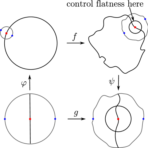
Figure 1. The relationship between $f$ and $g$

Let us now illustrate how to use Lemma 2.3 with quasispheres. Fix $\epsilon\in[0,1/20]$. Suppose that $f:\mathbb{R}^{n}\rightarrow\mathbb{R}^{n}$ is a quasiconformal map and suppose that there exists $r>0$ such that $\widetilde{H}_{f}(B(z,2r))\leq\epsilon$ for all $z\in S^{n-1}$. Pick $z\in S^{n-1}$ (the red square point in the upper left of Figure 1), let $\vec{n}_{z}$ denote a unit normal vector to $S^{n-1}$ at $z$, and assign $e^{r}_{\pm}=z\pm r\vec{n}_{z}$ (the blue round points). Choose any affine transformation $\varphi:\mathbb{R}^{n}\rightarrow\mathbb{R}^{n}$, which is a composition of a translation, a rotation and a dilation and such that $\varphi(0)=z$ and $\varphi(\pm e_{1})=e^{r}_{\pm}$. Then choose another affine transformation $\psi:\mathbb{R}^{n}\rightarrow\mathbb{R}^{n}$, which is a composition of a translation, a rotation and a dilation and such that $\psi((f(e_{+}^{r})+f(e_{-}^{r}))/2)=0$ and $\psi(f(e^{r}_{\pm}))=\pm e_{1}$. Finally put $g=\psi\circ f\circ\varphi$. Then $g|_{B(0,2)}$ is weakly $H_{f}(B(z,2r))$-quasisymmetric and $g(\pm e_{1})=\pm e_{1}$. By Lemma 2.3, $\theta_{g(e_{1}^{\perp})}(g(0),1/2)\leq 20\widetilde{H}_{f}(B(z,2r))$. Hence, letting $L_{z}$ denote the tangent plane to $S^{n-1}$ at $z$, this is equivalent to $\theta_{\psi\circ f(L_{z})}(\psi(f(z)),1/2)\leq 20\widetilde{H}_{f}(B(z,2r))$. Since the dilation factor of $\psi^{-1}$ is $|f(e^{r}_{+})-f(e^{r}_{-})|/2$, it follows that

(2.18) $$\theta_{f(L_{z})}\left(f(z),\frac{1}{4}|f(e^{r}_{+})-f(e^{r}_{-})|\right)\leq 20\widetilde{H}_{f}(B(z,2r)).$$

Since Lemma 2.3 also implies that $g(B(0,1))\supset B(g(0),5/6)$, we similarly get that

(2.19) $$f(B(z,r))\supset B\left(f(z),\frac{5}{12}|f(e^{r}_{+})-f(e^{r}_{-})|\right).$$

Notice that since $\widetilde{H}_{f}(B(z,2s))\leq\widetilde{H}_{f}(B(z,2r))$ for all $0<s\leq r$, a similar argument shows that (2.18) and (2.19) hold with $s$ in place of $r$ for all $0<s\leq r$.

We now apply the local Hölder continuity of the quasiconformal map $f$. Since $K_{f}(B(z,r))\leq H_{f}(B(z,r))^{n-1}\leq(1+\epsilon)^{n-1}$, there is a constant $C>1$ depending only on $n$ (because $0\leq\epsilon\leq 1/20$, e.g.  see Theorem 11.14 in [21] for a precise version of the local Hölder continuity we use here)

(2.20) $$|f(x)-f(y)|\leq CM_{z,r}|x-y|^{\alpha}\quad\text{for all }x,y\in B(z,r/2)$$

where $\alpha=(1+\epsilon)^{(n-1)/(1-n)}=(1+\epsilon)^{-1}$ and where $M_{z,r}=\sup_{|x-z|=r}|f(x)-f(z)|$. We also want to find a lower bound on $|f(x)-f(y)|$. First by two applications of weak quasisymmetry

(2.21) $$|f(e_{+}^{r})-f(e_{-}^{r})|\geq\frac{1}{1+\epsilon}|f(e_{+}^{r})-f(z)|\geq\left(\frac{1}{1+\epsilon}\right)^{2}M_{z,r}.$$

Combining (2.19) and (2.21), we conclude $f(B(z,r))$ contains $B(f(z),M_{z,r}/3)$. Thus, $K_{f^{-1}}(B(f(z),M_{z,r}/3))\leq K_{f}(B(z,r))\leq(1+\epsilon)^{n-1}$ and analogously to (2.20) we have that

(2.22) $$|f^{-1}(\xi)-f^{-1}(\eta)|\leq Cr|\xi-\eta|^{\alpha}\quad\text{for all }\xi,\eta\in B(f(z),M_{z,r}/6).$$

Suppose that we specified $r\leq r_{0}:=\min_{0\leq\epsilon\leq 1/20}2(1/6C)^{1/\alpha}$, which depends only on $n$. Then $|f(x)-f(z)|\leq M_{z,r}/6$ for all $x\in B(z,r/2)$ by (2.20). Thus, we can apply (2.22) with $x,y\in B(z,r/2)$, $\xi=f(x)$ and $\eta=f(y)$ to get that

(2.23) $$|x-y|\leq Cr_{0}|f(x)-f(y)|^{\alpha}\quad\text{for all }x,y\in B(z,r/2).$$

In particular, for all $0<s\leq r/2$,

(2.24) $$t=\frac{1}{4}|f(e_{+}^{s})-f(e_{-}^{s})|\geq\frac{1}{4}\left(\frac{2s}{Cr_{0}}\right)^{1/\alpha}=:c(2s)^{1/\alpha}.$$

Thus, since $2s\leq(t/c)^{\alpha}$ and $\widetilde{H}_{f}(B(z,\rho))$ is increasing in $\rho$, we conclude that

(2.25) $$\theta_{f(L_{z})}(f(z),t)\leq 20\widetilde{H}_{f}(B(z,(t/c)^{\alpha}))$$

for all $t>0$ such that $(t/c)^{\alpha}\leq r/2$. We remark that by replacing $c$ by $\min_{0\leq\epsilon\leq 1/20}c$, we may assert that $c$ depends only on $n$.

We now want to transfer the estimate (2.25) for the local flatness of the image $f(L_{z})$ of the tangent plane $L_{z}$ to an estimate for the quasicircle $f(S^{n-1})$. Evidently

(2.26) $$\begin{split}\theta_{f(S^{n-1})}(f(z),t)\leq&\ 20\widetilde{H}_{f}(B(z,(t/c)^{\alpha}))\\ &+\frac{1}{t}\mathop{\mathrm{missing}}{HD}[f(S^{n-1})\cap B(f(z),t),f(L_{z})\cap B(f(z),t)].\end{split}$$

Thus our next task is to estimate $\mathop{\mathrm{missing}}{HD}[f(S^{n-1})\cap B(f(z),t),f(L_{z})\cap B(f(z),t)]$. First we note that by elementary geometry there is an absolute constant $C_{0}$ so that

(2.27) $$\mathop{\mathrm{missing}}{HD}[S^{n-1}\cap B(z,\rho),L_{z}\cap B(z,\rho)]\leq C_{0}\rho^{2}\quad\text{for all }0<\rho\leq 1/2.$$

Thus, by the local Hölder continuity (2.20) and (2.23) and the constraint $0\leq\epsilon\leq 1/20$, there exist constants $c_{1}>0$ and $C_{1}>1$ that depend only on $n$ and $M_{z,r}$ so that

(2.28) $$\mathop{\mathrm{missing}}{HD}[f(S^{n-1})\cap B(f(z),c_{1}\rho^{1/\alpha}),f(L_{z})\cap B(f(z),c_{1}\rho^{1/\alpha})]\leq C_{1}\rho^{2\alpha}$$

for all $\rho>0$ such that $c_{1}\rho^{1/\alpha}\leq r/2$. With $t=c_{1}\rho^{1/\alpha}$, the estimate (2.28) becomes

(2.29) $$\mathop{\mathrm{missing}}{HD}[f(S^{n-1})\cap B(f(z),t),f(L_{z})\cap B(f(z),t)]\leq C_{2}t^{2\alpha^{2}}$$

where $C_{2}>1$ depends on $n$ and $M_{z,r}$. Substituting (2.29) into (2.26), we get that, for all $t>0$ sufficiently small,

(2.30) $$\theta_{f(S^{n-1})}(f(z),t)\leq 20\widetilde{H}_{f}(B(z,(t/c)^{\alpha}))+C_{2}t^{2\alpha^{2}-1}.$$

Observe that $\beta:=2\alpha^{2}-1\in(0,\alpha]$ since $0\leq\epsilon\leq 1/20$. Therefore, for all $t>0$ sufficiently small, $\widetilde{H}_{f}(B(z,(t/c)^{\alpha}))\leq\widetilde{H}_{f}(B(z,(t/c)^{\beta}))$ and

(2.31) $$\theta_{f(S^{n-1})}(f(z),t)\leq 20\widetilde{H}_{f}(B(z,(t/c)^{\beta}))+C_{2}t^{\beta}.$$

We have outlined the proof of the following theorem.

Theorem 2.4.

Let $f:\mathbb{R}^{n}\rightarrow\mathbb{R}^{n}$ be a quasiconformal map. If there exists $r>0$ such that $\widetilde{H}_{f}(B(z,2r))\leq\epsilon\leq 1/20$ for all $z\in S^{n-1}$, then there exist constants $c>0$ and $C>1$ depending only on $n$ and $M_{r}=\sup_{z\in S^{n-1}}\sup_{|x-z|=r}|f(x)-f(z)|$ and a constant $t_{0}>0$ depending only on $n$, $M_{r}$ and $r$ such that

(2.32) $$\sup_{z\in S^{n-1}}\theta_{f(S^{n-1})}(f(z),t)\leq 20\sup_{z\in S^{n-1}}\widetilde{H}_{f}(B(z,(t/c)^{\beta}))+Ct^{\beta}$$

for all $0<t\leq t_{0}$, where $\beta=2\alpha^{2}-1$, $\alpha=(1+\epsilon)^{-1}$.

Note that $\beta\uparrow 1$ as $\epsilon\downarrow 0$. Theorem 2.4 has several immediate consequences.

Corollary 2.5.

If $f:\mathbb{R}^{n}\rightarrow\mathbb{R}^{n}$ is quasiconformal and $\sup_{z\in S^{n-1}}\widetilde{H}_{f}(B(z,r))\rightarrow 0$ as $r\rightarrow 0$, then for all $0<\beta<1$ there exist constants $c,t_{0}>0$ and $C>1$ depending on $f$ and $\beta$ such that (2.32) holds for all $0<t\leq t_{0}$.

Corollary 2.6.

Let $0<\delta<1$. If $f:\mathbb{R}^{n}\rightarrow\mathbb{R}^{n}$ is a quasiconformal map and $\sup_{z\in S^{n-1}}\widetilde{H}_{f}(z,r)\leq\delta/40$ for some $r>0$, then $f(S^{n-1})$ is $(\delta,R)$-Reifenberg flat for some $R>0$.

Corollary 2.7.

If $f:\mathbb{R}^{n}\rightarrow\mathbb{R}^{n}$ is quasiconformal and $\sup_{z\in S^{n-1}}\widetilde{H}_{f}(B(z,r))\rightarrow 0$ as $r\rightarrow 0$ , then $f(S^{n-1})$ is Reifenberg flat with vanishing constant.

Remark 2.8.

Mattila and Vuorinen [9] demonstrated that sets with the $(\delta,R)$-linear approximation property (see [9] for the definition) have Hausdorff dimension at most $n-1+C\delta^{2}$, $C=C(n)>1$. Since $(\delta,R)$-Reifenberg flat sets also have the $(\delta,R)$-linear approximation property, Mattila and Vuorinen’s theorem and Corollary 2.6 imply the following bound. If $f:\mathbb{R}^{n}\rightarrow\mathbb{R}^{n}$ is quasiconformal, then

(2.33) $$\dim_{H}f(S^{n-1})\leq n-1+C\inf_{r>0}\sup_{z\in S^{n-1}}\left(\widetilde{H}_{f}(B(z,r))\right)^{2}.$$

On the other hand, every quasisphere has Hausdorff dimension at least $n-1$. Therefore, (1.16) and (2.33) imply that every asymptotically conformal quasisphere $f(S^{n-1})$ has Hausdorff dimension $n-1$.

We can now use Corollaries 2.2, 2.5 and 2.7 to prove Theorem 1.2.

Proof of Theorem 1.2.

Assume that $f:\mathbb{R}^{n}\rightarrow\mathbb{R}^{n}$ is a quasiconformal mapping such that (1.11) holds. Since the function $\sup_{z\in S^{n-1}}\widetilde{H}_{f}(B(z,\cdot))$ is decreasing, (1.11) implies that $\sup_{z\in S^{n-1}}\widetilde{H}_{f}(B(z,t))\rightarrow 0$ as $t\rightarrow 0$. Hence $f(S^{n-1})$ is Reifenberg flat with vanishing constant by Corollary 2.7. Pick any $\beta\in[1/2,1)$ and let $t_{0},c,C>0$ be the constants from Corollary 2.5 such that (2.32) holds. Since $(a+b)^{2}\leq 2a^{2}+2b^{2}$,

(2.34) $$\begin{split}&\int_{0}^{t_{0}}\sup_{z\in S^{n-1}}\left(\theta_{f(S^{n-1})}(f(z),t)\right)^{2}\frac{dt}{t}\\ &\qquad\leq 800\int_{0}^{t_{0}}\sup_{z\in S^{n-1}}\left(\widetilde{H}_{f}(B(z,(t/c)^{\beta}))\right)^{2}\frac{dt}{t}+2C^{2}\int_{0}^{t_{0}}t^{2\beta}\frac{dt}{t}.\end{split}$$

On one hand, using the change of variables $s=(t/c)^{\beta}$, $ds/s=(\beta/c)(dt/t)$,

(2.35) $$\begin{split}&\int_{0}^{t_{0}}\sup_{z\in S^{n-1}}\left(\widetilde{H}_{f}(B(z,(t/c)^{\beta}))\right)^{2}\frac{dt}{t}\\ &\qquad=\frac{c}{\beta}\int_{0}^{(t_{0}/c)^{\beta}}\sup_{z\in S^{n-1}}\left(\widetilde{H}_{f}(B(z,s))\right)^{2}\frac{ds}{s}<\infty\end{split}$$

by (1.11). On the other hand, since $\beta\geq 1/2$, $\int_{0}^{t_{0}}t^{2\beta-1}dt<\infty$. Therefore,

(2.36) $$\int_{0}^{t_{0}}\sup_{z\in S^{n-1}}\left(\theta_{f(S^{n-1})}(f(z),t)\right)^{2}\frac{dt}{t}<\infty,$$

and the quasisphere $f(S^{n-1})$ admits local $(1+\delta)$-bi-Lipschitz parameterizations for every $\delta>0$ by Corollary 2.2. It follows that $f(S^{n-1})$ is $(n-1)$-rectifiable. Moreover, since $f(S^{n-1})$ is compact, we conclude $\mathcal{H}^{n-1}(f(S^{n-1}))<\infty$. ∎

3. Local Bounds on Quasisymmetry

In this section, our goal is to derive Theorem 1.1 from Theorem 1.2. However, we face a technical challenge. We need to use the maximal dilatation of $f$ near $S^{n-1}$ to bound the weak quasisymmetry constant of $f$ near $S^{n-1}$. Our solution to this puzzle is Theorem 3.1.

Theorem 3.1.

Given $n\geq 2$ and $1<K\leq\min\{4/3,K^{\prime}\}$, set

(3.1) $$R=\left(\frac{c}{K-1}\right)^{c/(K-1)}$$

where $c>1$ is a constant that only depends on $n$ and $K^{\prime}$. Assume that $f:\mathbb{R}^{n}\rightarrow\mathbb{R}^{n}$ is $K^{\prime}$-quasiconformal. If, in addition, $K_{f}(B(w,Rs))\leq K$, then

(3.2) $$\widetilde{H}_{f}(B(w,s))\leq C(K-1)\log\left(\frac{1}{K-1}\right)$$

where $C>1$ is an absolute constant.

Corollary 3.2.

If $f:\mathbb{R}^{n}\rightarrow\mathbb{R}^{n}$ is quasiconformal and $\widetilde{K}_{f}(A_{t})\rightarrow 0$ as $t\rightarrow 0$, then $\sup_{z\in S^{n-1}}\widetilde{H}_{f}(B(z,t))\rightarrow 0$ as $t\rightarrow 0$.

Before we prove Theorem 3.1, let’s use it to establish Theorem 1.1.

Proof of Theorem 1.1.

Suppose that $f:\mathbb{R}^{n}\rightarrow\mathbb{R}^{n}$ is a $K^{\prime}$-quasiconformal map satisfying (1.5). We need to verify that $f$ also satisfies the Dini condition (1.11). Fix $z\in S^{n-1}$. In order to apply Theorem 3.1 and perform a change of variables at a certain step below, we choose a majorant $M(t)$ of $\widetilde{K}_{f}(A_{t})$ on $(0,r_{0})$, as follows. If $\widetilde{K}_{f}(A_{r})=0$ for some $r>0$, then set $r_{0}=r$ and let $M(t)=t$ for all $0<t<r_{0}$. Otherwise, let $r_{0}=1$ and let $M(t)$ any smooth increasing function such that

(3.3) $$\widetilde{K}_{f}(A_{t})\leq M(t)\leq b\widetilde{K}_{f}(A_{t})\quad\text{for all }0<t<1$$

for some constant $b>1$. (We note that $M(t)$ and $b$ exist by standard techniques. Also the constant $b$ depends only on $\widetilde{K}_{f}(A_{1})$ and hence is fully determined by $K^{\prime}$.) In both cases, $M(t)$ is a smooth increasing function such that $\lim_{t\rightarrow 0+}M(t)=0$, such that $\sup_{z\in S^{n-1}}\widetilde{K}_{f}(B(z,t))\leq\widetilde{K}_{f}(A_{t})\leq M(t)$ for all $0<t<r_{0}$ and such that

(3.4) $$\int_{0}^{r_{0}}\left(M(t)\log\frac{1}{M(t)}\right)^{2}\frac{dt}{t}<\infty.$$

By Theorem 3.1, there exist constants $c,C>1$ which depend only on $n$ and $K^{\prime}$ such that for all $t>0$ satisfying $M(t)\leq\min\{1/3,K^{\prime}-1\}$,

(3.5) $$\sup_{z\in S^{n-1}}\widetilde{H}_{f}(B(z,\phi(t)))\leq CM(t)\log\left(\frac{1}{M(t)}\right)$$

where

(3.6) $$\phi(t)=t\left(\frac{M(t)}{c}\right)^{c/M(t)}.$$

Since $M(t)\rightarrow 0$ as $t\rightarrow 0$, there is $t_{0}\in(0,r_{0})$ such that (3.5) holds for all $0<t\leq t_{0}$. Write $\psi(t)=M(t)/c$, so that $\phi(t)=t\exp\left(\frac{1}{\psi(t)}\log\psi(t)\right)$. Then

(3.7) $$\phi^{\prime}(t)=\exp\left(\frac{1}{\psi(t)}\log\psi(t)\right)\left[1+t\frac{\psi^{\prime}(t)}{\psi(t)^{2}}\left(1+\log\frac{1}{\psi(t)}\right)\right]$$

and

(3.8) $$\frac{\phi^{\prime}(t)}{\phi(t)}=\frac{1}{t}+\frac{\psi^{\prime}(t)}{\psi(t)^{2}}\left(1+\log\frac{1}{\psi(t)}\right).$$

Notice that since $M(t)$ is increasing and $M(t)\rightarrow 0$ as $t\rightarrow 0$, we have $\phi^{\prime}(t)>0$ for all $t$ sufficiently small. Thus, we can apply a change of variables $s=\phi(t)$, $ds/s=(\phi^{\prime}(t)/\phi(t))dt$ to obtain

(3.9) $$\begin{split}\int_{0}^{\phi(t_{0})}\sup_{z\in S^{n-1}}\left(\widetilde{H}_{f}(B(z,s))\right)^{2}\frac{ds}{s}&=\int_{0}^{t_{0}}\sup_{z\in S^{n-1}}\left(\widetilde{H}_{f}(B(z,\phi(t)))\right)^{2}\frac{\phi^{\prime}(t)}{\phi(t)}dt\\ &\leq C^{2}\int_{0}^{t_{0}}\left(M(t)\log\frac{1}{M(t)}\right)^{2}\frac{\phi^{\prime}(t)}{\phi(t)}dt.\end{split}$$

To establish (1.11), it remains to show that the integral on the right hand side of (3.9) is finite. Using (3.8) the integral on the right hand side of (3.9) is equal to

(3.10) $$\int_{0}^{t_{0}}\left(M(t)\log\frac{1}{M(t)}\right)^{2}\frac{dt}{t}+c^{2}\int_{0}^{t_{0}}\left(\log\frac{1}{c\psi(t)}\right)^{2}\left(1+\log\frac{1}{\psi(t)}\right)\psi^{\prime}(t)dt.$$

The first term on the right hand side of (3.10) is finite by (3.4). And, after changing variables again, the second term on the right hand side of (3.10) becomes

(3.11) $$c^{2}\int_{0}^{\psi(t_{0})}\left(\log\frac{1}{ct}\right)^{2}\left(1+\log\frac{1}{t}\right)dt,$$

which is finite too. This verifies (1.11). Therefore, by Theorem 1.2, the quasisphere $f(S^{n-1})$ admits local $(1+\delta)$-bi-Lipschitz parameterizations for every $\delta>0$.∎

It remains to prove Theorem 3.1. Rather than estimate the weak quasisymmetry constant $H_{f}(B(w,s))$ directly, we shall instead estimate a related extremal problem for standardized quasiconformal maps.

Definition 3.3.

1. We say that a quasiconformal map $g:\mathbb{R}^{n}\rightarrow\mathbb{R}^{n}$ is standardized if $g(0)=0$, $g(e_{1})=e_{1}$, and $g(B(0,1))\subset B(0,1)$.

2. Let $f:\mathbb{R}^{n}\rightarrow\mathbb{R}^{n}$ be any quasiconformal map, let $x\in\mathbb{R}^{n}$ and let $r>0$. A quasiconformal map $g:\mathbb{R}^{n}\rightarrow\mathbb{R}^{n}$ is a standardization of $f$ with respect to $B(x,r)$ if there exist affine transformations $\phi$ and $\psi$ of $\mathbb{R}^{n}$ such that $\phi(B(0,1))=B(x,r)$ and $g=\psi\circ f\circ\phi$ is standardized.

Remark 3.4 (How to Estimate $H_{f}(B(w,s)$).

Let $f:\mathbb{R}^{n}\rightarrow\mathbb{R}^{n}$ be $K^{\prime}$-quasiconformal, let $R>1$ and assume that $K_{f}(B(w,Rs))\leq K$. Suppose that we want to estimate $|f(\tilde{x})-f(\tilde{z})|/|f(\tilde{y})-f(\tilde{z})|$ for some $\tilde{x},\tilde{y},\tilde{z}\in B(w,s)$ with $|\tilde{x}-\tilde{z}|\leq|\tilde{y}-\tilde{z}|$. Then, writing $r:=|\tilde{y}-\tilde{z}|$, $B(\tilde{z},r)\subset B(w,3s)$, $K_{f}(B(\tilde{z},\frac{R}{3}r))\leq K$ and

(3.12) $$\begin{split}\frac{|f(\tilde{x})-f(\tilde{z})|}{|f(\tilde{y})-f(\tilde{z})|}&\leq\max\left\{\frac{|f(x)-f(\tilde{z})|}{|f(y)-f(\tilde{z})|}:|x-\tilde{z}|\leq|y-\tilde{z}|=r\right\}\\ &=\max\left\{\frac{|f(x)-f(\tilde{z})|}{|f(y)-f(\tilde{z})|}:|x-\tilde{z}|=|y-\tilde{z}|=r\right\}.\end{split}$$

Suppose that the maximum in (3.12) is obtained at $x=x^{\star}$ and $y=y^{\star}$. This implies that $|f(x^{\star})-f(\tilde{z})|\geq|f(y)-f(\tilde{z})|$ for all $y$ such that $|y-\tilde{z}|=r$. Let $\phi$ be any affine transformation of $\mathbb{R}^{n}$ sending $B(0,1)$ to $B(\tilde{z},r)$ with $\phi(0)=\tilde{z}$ and $\phi(e_{1})=x^{\star}$, and let $\psi$ be any affine transformation of $\mathbb{R}^{n}$ sending $B(f(\tilde{z}),|f(x^{\star})-f(\tilde{z})|)$ to $B(0,1)$ with $\psi(f(\tilde{z}))=0$ and $\psi(f(x^{\star}))=e_{1}$. Then $F=\psi\circ f\circ\phi$ is a standardization of $f$ with respect to $B(\tilde{z},r)$, $f$ is $K^{\prime}$-quasiconformal, $K_{F}(B(0,R/3))\leq K$ and

(3.13) $$\frac{|f(\tilde{x})-f(\tilde{z})|}{|f(\tilde{y})-f(\tilde{z})|}\leq\frac{|F(e_{1})-F(0)|}{|F(\phi^{-1}(y^{\star}))-F(0)|}=\frac{|F(e_{1})|}{|F(\phi^{-1}(y^{\star}))|}$$

where $|\phi^{-1}(y^{\star})|=1$. Let $\mathcal{G}(K^{\prime},K,R/3)$ denote the collection of all standardized $K^{\prime}$-quasiconformal maps $g$ such that $K_{g}(B(0,R/3))\leq K$. Then

(3.14) $$\frac{|f(\tilde{x})-f(\tilde{z})|}{|f(\tilde{y})-f(\tilde{z})|}\leq\max\left\{\frac{|g(x)|}{|g(y)|}:g\in\mathcal{G}(K^{\prime},K,R/3),\,|x|=|y|=1\right\}.$$

Therefore, since the right hand side of (3.14) is independent of $\tilde{x}$, $\tilde{y}$ and $\tilde{z}$,

(3.15) $$H_{f}(B(w,s))\leq\max\left\{\frac{|g(x)|}{|g(y)|}:g\in\mathcal{G}(K^{\prime},K,R/3),\,|x|=|y|=1\right\}$$

for every $K^{\prime}$-quasiconformal map $f$ of $\mathbb{R}^{n}$ such that $K_{f}(B(w,Rs))\leq K$.

The extremal problem described in Remark 3.4 (3.15) has been studied in the special case $K=K^{\prime}$ by several authors; see Vuorinen [22], Seittenranta [17], and most recently, Prause [12]. Our idea to prove Theorem 3.1 is to modify the method from [22] to incorporate two estimates on the maximal dilatation ($K_{g}(\mathbb{R}^{n})\leq K^{\prime}$ and $K_{g}(B(0,R/3))\leq K$). To do this we need to work with the geometric definition of quasiconformal maps. Recall that according to the geometric definition a map $f:\Omega\rightarrow\Omega^{\prime}$ between domains $\Omega,\Omega^{\prime}\subset\mathbb{R}^{n}$ is $K$-quasiconformal ($1\leq K<\infty$) provided that $f$ is a homeomorphism and the inequalities

(3.16) $$K^{-1}\mathrm{mod}_{n}(\Gamma)\leq\mathrm{mod}_{n}(f\Gamma)\leq K\mathrm{mod}_{n}(\Gamma)$$

hold for every curve family $\Gamma$ in $\Omega$. Here $\mathrm{mod}_{n}(\Gamma)$ refers to the $n$-modulus of $\Gamma$; e.g., see Heinonen [7]. We also define the maximal dilatation $K_{f}(\Omega)$ to be the smallest $K$ such that the inequalities (3.16) hold for all $\Gamma$. It is well known that the analytic and geometric definitions of quasiconformal maps coincide; e.g., see Chapter 4, §36 of Väisälä [20].

As a preliminary step towards the proof of Theorem 3.1, we record some facts about the modulus of the Teichmüller ring $[-e_{1},0]\cup[se_{1},\infty]$ in $\mathbb{R}^{n}$ with $s>0$ and the Grötzsch ring $\overline{B(0,1)}\cup[te_{1},\infty)$ in $\mathbb{R}^{n}$ with $t>1$. For every pair of disjoint sets $E,F\subset\mathbb{R}^{n}$, $(E,F)$ is the family of curves connecting $E$ and $F$ in $\mathbb{R}^{n}$.

Lemma 3.5.

With $n\geq 2$ fixed, assign $\tau_{n}(s)=\mathrm{mod}_{n}([-e_{1},0],[se_{1},\infty))$ for all $s>0$, and assign $\gamma_{n}(t)=\mathrm{mod}_{n}(B(0,1),[te_{1},\infty))$ for all $t>1$. The functions $\tau_{n}$ and $\gamma_{n}$ are decreasing homeomorphisms onto $(0,\infty)$. Moreover,

(3.17) $$\gamma_{n}(t)=2^{n-1}\tau_{n}(t^{2}-1)\quad\text{for all }t>1$$

and

(3.18) $$\frac{\sigma_{n-1}}{\left(\log\lambda_{n}t\right)^{n-1}}\leq\gamma_{n}(t)\leq\frac{\sigma_{n-1}}{\left(\log t\right)^{n-1}}\quad\text{for all $t>1$}$$

where $\sigma_{n-1}=\mathcal{H}^{n-1}(S^{n-1})$ is the surface area of the unit sphere and $\lambda_{n}\in[4,2e^{n-1})$ is the Grötzsch constant. For all $A>0$, define the distortion function

(3.19) $$\varphi_{A,n}(r)=\frac{1}{\gamma_{n}^{-1}(A\gamma_{n}(1/r))}\quad\text{for all $0<r<1$}.$$

Then $\varphi_{n,A}$ is an increasing homeomorphism from $(0,1)$ to $(0,1)$.

Proof.

We refer the reader to §7 of Vuorinen [21].∎

In the special case $K=K^{\prime}$, the following calculation appears in slightly different form in Seittenranta [17] (c.f. Theorem 1.5 and Lemma 3.1 in [17]) and Prause [12] (c.f. Theorem 2.7 and Theorem 3.1 in [12]).

Lemma 3.6.

Let $\mathcal{G}_{R}=\mathcal{G}(K^{\prime},K,R)$ be the family of standardized $K^{\prime}$-quasiconformal maps $g:\mathbb{R}^{n}\rightarrow\mathbb{R}^{n}$ such that $K_{g}(B(0,R))\leq K$. For all $1<A\leq 16/9$ there exists $t_{0}\in(0,1)$ (see (3.28)) depending only on $n$ and $A$ such that if the inequalities

(3.20) $$\gamma_{n}\left(\sqrt{1+\frac{1}{|g(x)|}}\right)\leq A\gamma_{n}\left(\sqrt{\frac{1}{|x|}}\right)$$

and

(3.21) $$\gamma_{n}\left(\sqrt{1+\frac{1}{|x|}}\right)\leq A\gamma_{n}\left(\sqrt{\frac{1}{|g(x)|}}\right)$$

hold for all $g\in\mathcal{G}_{R}$ and $|x|=t_{0}$, then

(3.22) $$\max\left\{\frac{|h(x)|}{|h(y)|}:h\in\mathcal{G}_{R/t_{0}},\,|x|=|y|=1\right\}\leq 1+C(A-1)\log\left(\frac{1}{A-1}\right).$$

for some absolute constant $C>1$.

Proof.

Let $n$, $K^{\prime}$, $K$, $R$ and $A$ be given and fix $t_{0}\in(0,1)$ to be specified later. Suppose that (3.20) and (3.21) hold for all $g\in\mathcal{G}_{R}$ when $|x|=t_{0}$. We remark that (3.20) and (3.21) make sense, since $0<|g(x)|<1$ when $0<|x|<1$ because $g$ is standardized. Since $\gamma_{n}$ is strictly decreasing, one can apply $\gamma^{-1}_{n}$ to both sides of (3.20), invoke the definition of the distortion function (3.19), and perform basic manipulations to get

(3.23) $$|g(x)|\leq\frac{\varphi_{A,n}^{2}(\sqrt{t_{0}})}{1-\varphi_{A,n}^{2}(\sqrt{t_{0}})}=:\mathcal{A}(t_{0})\quad\text{for all }g\in\mathcal{G}_{R}.$$

Similarly, after first dividing (3.21) through by $A$, one can apply $\gamma^{-1}_{n}$, use (3.19), and perform basic manipulations to get

(3.24) $$|g(x)|\geq\varphi_{1/A,n}^{2}\left(\sqrt{\frac{t_{0}}{1+t_{0}}}\right)=:\mathcal{B}(t_{0})\quad\text{for all }g\in\mathcal{G}_{R}.$$

Combining (3.23) and (3.24), we get that

(3.25) $$\frac{|g(x)|}{|g(y)|}\leq\frac{\mathcal{A}(t_{0})}{\mathcal{B}(t_{0})}\quad\text{for all }g\in\mathcal{G}_{R}\text{ and }|x|=|y|=t_{0}.$$

Since

(3.26) $$\left\{\frac{|h(x)|}{|h(y)|}:h\in\mathcal{G}_{R/t_{0}},|x|=|y|=1\right\}=\left\{\frac{|g(x)|}{|g(y)|}:g\in\mathcal{G}_{R},\,|x|=|y|=t_{0}\right\},$$

we conclude that

(3.27) $$\max\left\{\frac{|h(x)|}{|h(y)|}:h\in\mathcal{G}_{R/t_{0}},\,|x|=|y|=1\right\}\leq\frac{\mathcal{A}(t_{0})}{\mathcal{B}(t_{0})}.$$

Ideally one would like to choose $t_{0}$ which minimizes the right hand side of (3.27). Unfortunately, this critical value of $t_{0}$ cannot be solved for algebraically. Instead, following Vuorinen [22], Seittenranta [17] and Prause [12] we take

(3.28) $$t_{0}=\left(\lambda_{n}^{2(\alpha-1)}\frac{A-1}{A}\right)^{\beta}\quad\text{where }\alpha=A^{1/(1-n)},\ \beta=A^{1/(n-1)}.$$

By Lemma 3.1 in [17], if $1<A\leq 2$, then

(3.29) $$\frac{\mathcal{A}(t_{0})}{\mathcal{B}(t_{0})}\leq\exp\left(\left(4\sqrt{2}+\log\frac{1}{A-1}\right)(A^{2}-1)\right).$$

If $1<A\leq 16/9$, then $4\sqrt{2}\leq 23\log(1/(A-1))$ and $(A^{2}-1)\leq 3(A-1)$. Thus,

(3.30) $$\frac{\mathcal{A}(t_{0})}{\mathcal{B}(t_{0})}\leq\exp\left(72(A-1)\log\frac{1}{A-1}\right)$$

Finally note $72(A-1)\log(1/(A-1))$ is bounded for $1<A\leq 16/9$ and $e^{x}\leq 1+e^{b}x$ when $x\leq b$. Therefore, from (3.27) and (3.30), it readily follows that

(3.31) $$\max\left\{\frac{|h(x)|}{|h(y)|}:h\in\mathcal{G}_{R/t_{0}},\,|x|=|y|=1\right\}\leq 1+C(A-1)\log\left(\frac{1}{A-1}\right)$$

for some absolute constant $C>1$, whenever $1<A\leq 16/9$. ∎

As a model for Theorem 3.1, let us now verify (1.15). Suppose that $f:\mathbb{R}^{n}\rightarrow\mathbb{R}^{n}$ is a $K^{\prime}$-quasiconformal map (with $K^{\prime}$ near 1) and assume $f$ is standardized so that $f(0)=0$ and $f(e_{1})=e_{1}$, and $0<|f(x)|<1$ whenever $0<|x|<1$. Following Vuorinen [22], we fix a point $x$ with $|x|\in(0,1)$ and consider the following four curve families in $\mathbb{R}^{n}$ (see Figure 2):

• $\Delta=([0,x],[e_{1},\infty))$,

• $\Delta^{*}=([0,|x|e_{1}],[e_{1},\infty))$,

• $f(\Delta)=(f[0,x],f[e_{1},\infty))$,

• $f(\Delta)_{*}=([-|f(x)|e_{1},0],[e_{1},\infty))$.

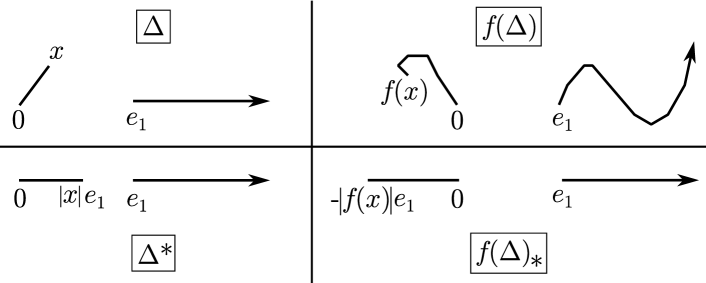
Figure 2. Families of curves

The modulus of these curve families are related by

(3.32) $$\mathrm{mod}_{n}(f(\Delta)_{*})\leq\mathrm{mod}_{n}(f(\Delta))\leq K^{\prime}\mathrm{mod}_{n}(\Delta)\leq K^{\prime}\mathrm{mod}_{n}(\Delta^{*}),$$

where the first inequality holds by spherical symmetrization (e.g. see §7 in [21]), the second inequality holds since $f$ is $K^{\prime}$-quasiconformal, and the third inequality is a lemma of Gehring (see Lemma 5.27 in [21]). The rings $[-|f(x)|e_{1},0]\cup[e_{1},\infty)$ and $[0,|x|e_{1}]\cup[e_{1},\infty)$ used to define $f(\Delta)_{*}$ and $\Delta^{*}$, respectively, are conformally equivalent to Teichmüller rings by translation and dilation. Thus using the modulus of Teichmüller rings we can rewrite (3.32) as

(3.33) $$\tau_{n}\left(\frac{1}{|f(x)|}\right)\leq K^{\prime}\tau_{n}\left(\frac{1}{|x|}-1\right).$$

Thus, using (3.17),

(3.34) $$\gamma_{n}\left(\sqrt{1+\frac{1}{|f(x)|}}\right)\leq K^{\prime}\gamma_{n}\left(\sqrt{\frac{1}{|x|}}\right).$$

Applying a similar argument with $f^{-1}$ instead of $f$ and $y=f(x)$ instead of $x$ yields

(3.35) $$\gamma_{n}\left(\sqrt{1+\frac{1}{|x|}}\right)\leq K^{\prime}\gamma_{n}\left(\sqrt{\frac{1}{|f(x)|}}\right).$$

Notice that $\mathcal{G}=\mathcal{G}(K^{\prime},K^{\prime},R)$ is independent of $R>0$. Since (3.34) and (3.35) hold for all $f\in\mathcal{G}$ and for all $x$ such that $|x|\in(0,1)$, Lemma 3.6 yields

(3.36) $$\max\left\{\frac{|g(x)|}{|g(y)|}:g\in\mathcal{G},\,|x|=|y|=1\right\}\leq 1+C(K^{\prime}-1)\log\left(\frac{1}{K^{\prime}-1}\right).$$

Thus, by Remark 3.4, if $f:\mathbb{R}^{n}\rightarrow\mathbb{R}^{n}$ is $K^{\prime}$-quasiconformal (with $K^{\prime}$ near 1), then

(3.37) $$\widetilde{H}_{f}(B(w,s))\leq C(K^{\prime}-1)\log\left(\frac{1}{K^{\prime}-1}\right)\quad\text{for all }w\in\mathbb{R}^{n}\text{ and }s>0.$$

Since the right hand side is independent of $w$ and $s$, (3.37) implies (1.15).

We will now rerun this argument, with modifications designed to utilize two estimates on the maximal dilatation of $f$.

Proof of Theorem 3.1.

Let constants $K$ and $K^{\prime}$ satisfying $1<K\leq\min\{4/3,K^{\prime}\}$ be given. Fix $R>1$ to be specified later (see (3.53)) and choose $f\in\mathcal{G}(K^{\prime},K,R)$. Then $f:\mathbb{R}^{n}\rightarrow\mathbb{R}^{n}$ is a standardized $K^{\prime}$-quasiconformal map and $K_{f}(B(0,R))\leq K$. Fix $x\in B(0,1)\setminus\{0\}$ and let $\Delta$, $\Delta^{*}$, $f(\Delta)$ and $f(\Delta)_{*}$ be the curve families associated to $x$ defined above. Furthermore, decompose $\Delta$ as the union of two curve families,

(3.38) $$\Delta=\Gamma_{1}\cup\Gamma_{2},$$

where $\Gamma_{1}$ consists of all curves in $\Delta$ which remain inside $B(0,R)$ and $\Gamma_{2}=\Delta\setminus\Gamma_{1}$ (see Figure 3).

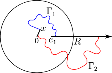
Figure 3. Curves in $\Gamma_{1}$ and $\Gamma_{2}$

Continuing as above, and using the subadditivity of modulus,

(3.39) $$\mathrm{mod}_{n}(f(\Delta)_{*})\leq\mathrm{mod}_{n}(f(\Delta))\leq\mathrm{mod}_{n}(f(\Gamma_{1}))+\mathrm{mod}_{n}(f(\Gamma_{2})).$$

On one hand, since curves in $\Gamma_{1}$ lie inside $B(0,R)$, the estimate $K_{f}(B(0,R))\leq K$ on the maximal dilatation yields

(3.40) $$\mathrm{mod}_{n}(f(\Gamma_{1}))\leq K\mathrm{mod}_{n}(\Gamma_{1})\leq K\mathrm{mod}_{n}(\Delta)\leq K\mathrm{mod}_{n}(\Delta^{*}).$$

On the other hand, let $\Gamma(r,R)$ be the family of all curves connecting $\partial B(0,r)$ to $\partial B(0,R)$ in $B(0,R)\setminus B(0,r)$. This is one of the few curve families where the modulus is explicitly known (e.g. see [21]): $\rho_{n}(r,R):=\mathrm{mod}_{n}(\Gamma(r,R))=\sigma_{n-1}(\log R/r)^{1-n}$. Because every curve in $\Gamma_{2}$ has a subcurve which belongs to $\Gamma(1,R)$,

(3.41) $$\mathrm{mod}_{n}(f(\Gamma_{2}))\leq K^{\prime}\mathrm{mod}_{n}(\Gamma_{2})\leq K^{\prime}\mathrm{mod}_{n}(\Gamma(1,R))=K^{\prime}\rho_{n}(1,R).$$

Combining (3.39), (3.40) and (3.41) gives

(3.42) $$\mathrm{mod}_{n}(f(\Delta)_{*})\leq K\mathrm{mod}_{n}(\Delta^{*})+K^{\prime}\rho_{n}(1,R).$$

Rewriting (3.42) using the modulus of Grötzsch rings, we get

(3.43) $$\gamma_{n}\left(\sqrt{1+\frac{1}{|f(x)|}}\right)\leq K\gamma_{n}\left(\sqrt{\frac{1}{|x|}}\right)+K^{\prime}\rho_{n}(1,R).$$

One may view (3.43) as an analogue of (3.34). We want to find a similar analogue for (3.35). We now use the global Hölder continuity of the quasiconformal map $f$. Since $f:\mathbb{R}^{n}\rightarrow\mathbb{R}^{n}$ is $K^{\prime}$-quasiconformal, $f(0)=0$ and $f(e_{1})=e_{1}$, there exists a constant $M>1$ depending only on $n$ and $K^{\prime}$ such that

(3.44) $$M^{-1}\min\{|z|^{\alpha^{\prime}},|z|^{\beta^{\prime}}\}\leq|f(z)|\leq M\max\{|z|^{\alpha^{\prime}},|z|^{\beta^{\prime}}\}\quad\text{for all }z\in\mathbb{R}^{n}$$

where $\alpha^{\prime}=(K^{\prime})^{1/(1-n)}$ and $\beta^{\prime}=(K^{\prime})^{1/(n-1)}$; for this version of Hölder continuity for normalized quasiconformal maps, see Theorem 1.8(3) in [22]. In particular, (3.44) implies that $f(B(0,R))\supset B(0,R^{\alpha^{\prime}}/M)$. Hence $K_{f^{-1}}(B(0,R^{\alpha^{\prime}}/M))\leq K$. Thus, if $R>1$ is sufficiently large to ensure $R^{\alpha^{\prime}}/M>1$, then by arguing as above with $f^{-1}$ instead of $f$ and $y=f(x)$ instead of $x$ we get

(3.45) $$\gamma_{n}\left(\sqrt{1+\frac{1}{|x|}}\right)\leq K\gamma_{n}\left(\sqrt{\frac{1}{|f(x)|}}\right)+K^{\prime}\rho_{n}(1,R^{\alpha^{\prime}}/M)$$

for all $x\in B(0,1)\setminus\{0\}$.

Our next task is to choose $R>1$ so large that we can absorb the $\rho_{n}$-terms in (3.43) and (3.45) into the $\gamma_{n}$-terms. Let

(3.46) $$t_{0}=\left(\lambda_{n}^{2(\alpha^{2}-1)}\frac{K^{2}-1}{K^{2}}\right)^{\beta^{2}}$$

be the constant from Lemma 3.6 associated to $A=K^{2}$, where $\alpha=K^{1/(1-n)}$ and $\beta=K^{1/(n-1)}$. Suppose that we can pick $R>1$ large enough to guarantee

(3.47) $$K^{\prime}\rho_{n}(1,R)\leq K(K-1)\gamma_{n}\left(\sqrt{\frac{1}{|x|}}\right)$$

and

(3.48) $$K^{\prime}\rho_{n}(1,R^{\alpha^{\prime}}/M)\leq K(K-1)\gamma_{n}\left(\sqrt{\frac{1}{|f(x)|}}\right)$$

for all $x$ such that $|x|=t_{0}$. Then, combining (3.43), (3.45), (3.47) and (3.48), we see that (3.20) and (3.21) hold with $A=K^{2}$ for all $f\in\mathcal{G}(K^{\prime},K,R)$ and for all $x$ such that $|x|=t_{0}$. Therefore, since $1<K^{2}\leq 16/9$, Lemma 3.6 will imply that

(3.49) $$\begin{split}\max\left\{\frac{|h(x)|}{|h(y)|}:h\in\mathcal{G}_{R/t_{0}},\,|x|=|y|=1\right\}&\leq 1+C(K^{2}-1)\log\left(\frac{1}{K^{2}-1}\right)\\ &\leq 1+3C(K-1)\log\left(\frac{1}{K-1}\right)\end{split}$$

for some absolute constant $C>1$.

Let us now find how large $R>1$ must be to ensure that (3.47) and (3.48) hold. First observe that if $|x|=t_{0}$ then $\sqrt{1/|f(x)|}\leq(M/t_{0}^{\beta^{\prime}})^{1/2}$ by (3.44). Hence, since $\gamma_{n}$ is decreasing, (3.48) will hold provided that

(3.50) $$K^{\prime}\rho_{n}(1,R^{\alpha^{\prime}}/M)\leq K(K-1)\gamma_{n}\left((M/t_{0}^{\beta^{\prime}})^{1/2}\right).$$

Using the formula for $\rho_{n}(1,R^{\alpha^{\prime}}/M)$ from above and the first inequality in (3.18), we see that (3.47) and (3.50) will hold if

(3.51) $$K^{\prime}\sigma_{n-1}\left(\log R\right)^{1-n}\leq K(K-1)\sigma_{n-1}\left(\log\lambda_{n}(1/t_{0})^{1/2}\right)^{1-n}$$

and

(3.52) $$K^{\prime}\sigma_{n-1}\left(\log R^{\alpha^{\prime}}/M\right)^{1-n}\leq K(K-1)\sigma_{n-1}\left(\log\lambda_{n}(M/t_{0}^{\beta^{\prime}})^{1/2}\right)^{1-n},$$

respectively. From here an undaunted reader can verify using elementary operations that there is a constant $c>1$ depending only on $n$ and $K^{\prime}$ so that the inequalities (3.51) and (3.52) hold whenever

(3.53) $$R\geq\left(\frac{c}{K-1}\right)^{c/(K-1)}.$$

For definiteness, let $c>1$ be the smallest constant such that (3.53) implies (3.52) for all $1<K\leq 4/3$ and set $R=(c/(K-1))^{c/(K-1)}$. From our previous discussion, it follows that (3.49) holds with this choice of $R$. By Remark 3.4, we conclude that $\widetilde{H}_{f}(B(w,s))\leq 3C(K-1)\log\left(\frac{1}{K-1}\right)$ for every quasiconformal map $f:\mathbb{R}^{n}\rightarrow\mathbb{R}^{n}$ such that $K_{f}(B(w,3(R/t_{0})s))\leq K$. Finally observe that

(3.54) $$\frac{3R}{t_{0}}\leq\left(\frac{\tilde{c}}{K-1}\right)^{\tilde{c}/(K-1)}=:\widetilde{R}$$

for some constant $\tilde{c}\geq c$ depending only on $n$ and $K^{\prime}$. This completes the proof. ∎

References

[1] G.D. Anderson, M.K. Vamanamurthy, and M.K. Vuorinen, Conformal invariants, inequalities, and quasiconformal maps, Canadian Mathematical Society Series of Monographs and Advanced Texts, John Wiley & Sons, Inc., New York, 1997.
[2] J.M. Anderson, J. Becker, and F.D. Lesley, On the boundary correspondence of asymptotically conformal automorphisms, J. London Math. Soc. (2) 38 (1988), no. 3, 453–462.
[3] C.J. Bishop, V.Ya. Gutlyanskiĭ, O. Martio and M. Vuorinen, On conformal dilatation in space, Int. J. Math. Math. Sci. 2003, no. 22, 1397–1420.
[4] G. David and T. Toro, Reifenberg flat metric spaces, snowballs, and embeddings, Math. Ann. 315 (1999), no. 4, 641–710.
[5] G. David and T. Toro, Reifenberg parameterizations for sets with holes, Mem. Amer. Math. Soc. 215 (2012), no. 1012.
[6] V.Ya. Gutlyanskiĭ and A. Golberg, On Lipschitz continuity of quasiconformal mappings in space, J. Anal. Math. 109 (2009), 233–251.
[7] J. Heinonen, Lectures on analysis on metric spaces, Universitext, Springer-Verlag, New York, 2001.
[8] P.W. Jones, Rectifiable sets and the traveling salesman problem, Invent. Math. 102 (1990), no. 1, 1–15.
[9] P. Mattila and M. Vuorinen, Linear approximation property, Minkowski dimension, and quasiconformal spheres, J. London Math. Soc. (2) 42 (1990), no. 2, 249–266.
[10] D. Meyer, Quasisymmetric embedding of self similar surfaces and origami rational maps, Ann. Acad. Sci. Fenn. Math. 27 (2002), no. 2, 461–484.
[11] D. Meyer, Snowballs are quasiballs, Trans. Amer. Math. Soc. 362 (2010), no. 3, 1247–1300.
[12] I. Prause, Flatness properties of quasispheres, Comput. Methods Func. Theory 7 (2007), no. 2, 527–541.
[13] I. Prause, X. Tolsa, I. Uriarte-Tuero, Hausdorff measure of quasicircles, Adv. Math. 229 (2012), no. 2, 1313–1328.
[14] E. Reifenberg, Solution of the Plateau problem for -dimensional surface of varying topological type, Acta Math. 104 (1960), 1–92.
[15] Yu.G. Reshetnyak, Stability theorems in geometry and analysis, Mathematics and Its Applications, vol. 304, Kluwer Academic Publishers Group, Dordrecht, 1994.