A Bias-reduced Estimator for the Mean of a Heavy-tailed Distribution with an Infinite Second Moment

Abstract

We use bias-reduced estimators of high quantiles, of heavy-tailed distributions, to introduce a new estimator of the mean in the case of infinite second moment. The asymptotic normality of the proposed estimator is established and checked, in a simulation study, by four of the most popular goodness-of-fit tests for different sample sizes. Moreover, we compare, in terms of bias and mean squared error, our estimator with Peng’s estimator (Peng, 2001) and we evaluate the accuracy of some resulting confidence intervals.

Keywords: Bias reduction; Extreme values; Heavy-tailed distributions; Hill estimator; Regular variation; Tail index.

1 Introduction

Let $X_{1},X_{2},...$ be independent and identically distributed (i.i.d.) non-negative random variables (r.v.’s) with mean $\mu<\infty,$ variance $\sigma^{2}$ and cumulative distribution function (cdf) $F.\$Suppose that the tail of $F$ is regularly varying at infinity with tail index $\left(-\alpha\right)<0,$ that is

$$\lim_{t\rightarrow\infty}\frac{1-F\left(tx\right)}{1-F\left(t\right)}=x^{-\alpha},\text{ \ \ \ for any }x>0,$$ (1.1)

(see, e.g., [de Haan and Ferreria, (2006), , page 19]). Such cdf’s constitute a major subclass of the family of heavy-tailed distributions. It includes distributions such as Pareto, Burr, Student, $\alpha-$stable $\left(0<\alpha<2\right),$ and log–gamma, which are known to be appropriate models for fitting large insurance claims, large fluctuations of prices, log–returns, etc. (see, e.g. [Reiss and Thomas, (2007)]; [Beirlant et al. (2001)]; [Rolski et al. (1999)]). In this paper, we are concerned with the construction of a bias-reduced asymptotically normal estimator for the mean

$$\mu:=\int_{0}^{\infty}xdF\left(x\right),$$

which could be rewritten, in terms of the quantile function (corresponding to the cdf $F)$

$$Q(s):=\inf\left\{x:F\left(x\right)\geq s\right\},\text{ }0<s<1,$$

as

$$\mu=\int_{0}^{1}Q\left(1-s\right)ds.$$ (1.2)

For a given sample $X_{1},...,X_{n},$ let

$${\normalsize Q_{n}\left(s\right):=\inf\left\{x\in\mathbb{R}:F_{n}\left(x\right)\geq s\right\},\;0<s\leq 1,}$$

denote the sample quantile function (classical non-parametric estimator of $Q)\$associated to the empirical cdf defined on the real line by ${\normalsize F_{n}\left(x\right):=n}^{-1}\sum\nolimits_{i=1}^{n}\mathbb{I}\left(X_{i}\leq x\right),$ with $\mathbb{I}\left(\cdot\right)$ being the indicator function. The natural (unbiased) estimator of $\mu$ is the sample mean

$$\int_{0}^{1}Q_{n}\left(1-s\right)ds=\dfrac{1}{n}{\displaystyle\sum\limits_{i=1}^{n}}X_{i}=:\overline{X}_{n}\text{.}$$ (1.3)

From the Central Limit Theorem (CLT), the sequence of r.v.’s $\left\{\sqrt{n}\left(\overline{X}_{n}-\mu\right)/\sigma,\text{ }n\geq 1\right\}$ converges in distribution to the standard Gaussian r.v., provided that the second-order moment $\mathbf{E}\left[X_{1}^{2}\right]$ is finite. This is a very restrictive condition in the context of heavy-tailed distributions as the following considerations show. Assume that the r.v. $X_{1}$ follows the Pareto law with index $\alpha>0,$ that is, $1-F(x)=x^{-\alpha}$ for $x\geq 1$. When $\alpha>1,$ the mean $\mu$ exists, but $\mathbf{E}\left[X_{1}^{2}\right]$ is only finite for $\alpha\geq 2.$ Hence, the range $\alpha\in(1,2)$ is not covered by the CLT and thus we need to seek another approach to handle this situation. Making use of Weissman’s estimator of high quantiles [Weissman, (1978)], [Peng, (2001)] proposed an alternative estimator for $\mu$ and established its asymptotic normality for any $\alpha\in(1,2).$ Let us define the following estimator for $Q:$

$$\widehat{Q}_{n}(1-s):=\left\{\begin{array}[c]{lcc}Q_{n}^{W}(1-s)&\text{for }&0<s<k/n\vskip 6.0pt plus 2.0pt minus 2.0pt\\ Q_{n}(1-s)&\text{for}&k/n\leq s<1,\end{array}\right.$$

where

$$Q_{n}^{W}(1-s):=(k/n)^{1/\widehat{\alpha}_{n}^{H}}X_{n-k,n}s^{-1/\widehat{\alpha}_{n}^{H}},\text{ }s\downarrow 0$$ (1.4)

is Weissman’s estimator of high quantiles, with

$$\widehat{\alpha}_{n}^{H}:=\left(k^{-1}\sum\limits_{i=1}^{k}\log X_{n-i+1,n}-\log X_{n-k,n}\right)^{-1},$$ (1.5)

being the well-known Hill estimator [Hill, (1975)] of the tail index $\alpha,$ and $X_{1,n}\leq...\leq X_{n,n}$ denoting the order statistics pertaining to the sample $X_{1},...,X_{n}.$ The number $k$ represents the number of upper order statistics used in the computation of $\widehat{\alpha}_{n}^{H},$ it is an integer sequence $k=k_{n}$ satisfying

$$1<k<n,\text{ }k\rightarrow\infty\text{ and }k/n\rightarrow 0\text{ as }n\rightarrow\infty.$$ (1.6)

By replacing $Q\left(1-s\right)$ by $\widehat{Q}_{n}(1-t)$ in formula (1.2), [Peng, (2001)] proposed an alternative estimator for $\mu$ as follows:

$$\widehat{\mu}_{n}^{P}=\widehat{\mu}_{n}^{P}\left(k\right):=\int_{0}^{1}\widehat{Q}_{n}(1-s)ds=\int_{0}^{k/n}Q_{n}^{W}\left(1-s\right)ds+\int_{k/n}^{1}Q_{n}(1-s)ds,$$

which, by a straightforward calculation, is equal to

$$\widehat{\mu}_{n}^{P}:=\frac{k}{n}\frac{\widehat{\alpha}_{n}^{H}}{\widehat{\alpha}_{n}^{H}-1}X_{n-k,n}+\frac{1}{n}\sum_{i=k+1}^{n}X_{n-i+1,n},$$ (1.7)

provided that $\widehat{\alpha}_{n}^{H}>1.$ Moreover, the same author showed that, under suitable regularity assumptions, for any $\alpha\in(1,2),$

$$\frac{\sqrt{n}\left(\widehat{\mu}_{n}^{P}-\mu\right)}{\sqrt{k/n}X_{n-k,n}}\overset{d}{\rightarrow}\mathcal{N}\left(0,\sigma^{2}\left(\alpha\right)\right),\text{ as }n\rightarrow\infty,$$ (1.8)

where

$$\sigma^{2}\left(\alpha\right):=\alpha/\left(1-\alpha\right)^{4}\left(2-\alpha\right).$$

Throughout this paper, the standard notations $\overset{p}{\rightarrow},$ $\overset{d}{\rightarrow}$ and $\overset{d}{=}$ respectively stand for convergence in probability, convergence in distribution and equality in distribution, while $\mathcal{N}\left(a,b^{2}\right)$ denotes the normal distribution with mean $a$ and variance $b^{2}.\vskip 6.0pt plus 2.0pt minus 2.0pt$

Actually, [Peng, (2001)] defined his estimator in the more general situation where the r.v. $X$ is real (not necessarily non-negative) with lower and upper heavy tails. He simultaneously took into account the regular variations of both tails of $G$ and the balance condition

$$\lim_{t\rightarrow\infty}\left(1-F\left(t\right)\right)/\left(1-F\left(t\right)-F\left(-t\right)\right)=p\in\left[0,1\right].$$

In this paper, we only consider non-negative r.v.’s. Our motivation comes from the actuarial risk theory where insurance losses are represented by such r.v.’s. In this case, $\widehat{\mu}_{n}^{P}$ may be interpreted as an estimator of a risk measure called the net premium, see for instance [Necir and Meraghni, (2009)] and [Brahimi et al. (2011)]. Note that in our case, since r.v. $X$ is non-negative, we have $F\left(-x\right)=0$ for $x\geq 0,$ which yields $p=1$ in the above balance condition.

Hill’s estimator $\widehat{\alpha}_{n}^{H}$ plays a pivotal role in statistical inference on distribution tails. This estimator has been thoroughly studied, improved and even generalized to any real parameter $\alpha.$ Weak consistency of $\widehat{\alpha}_{n}^{H}$ was established by [Mason, (1982)] assuming only that the underlying cdf $F$ satisfies condition (1.1). The asymptotic normality of $\widehat{\alpha}_{n}^{H}$ has been established (see [de Haan and Peng, (1998)]) under the following stricter condition that characterizes Hall’s model (see [Hall, (1982)] and [Hall and Welsh, (1985)]).

$$1-F\left(x\right)=cx^{-\alpha}+dx^{-\beta}+o\left(x^{-\beta}\right),\text{ as }x\rightarrow\infty,$$ (1.9)

for some $c>0,$ $d\neq 0$ and $\beta>\alpha>0.$ Note that (1.9), which is a special case of a more general second-order regular variation condition (see [de Haan and Stadtmüller, (1996)]), is equivalent to

$$Q\left(1-s\right)=c^{1/\alpha}s^{-1/\alpha}\left(1+\alpha^{-1}c^{-\beta/\alpha}ds^{\beta/\alpha-1}+o\left(1\right)\right),\text{ as }s\downarrow 0.$$ (1.10)

The constants $\alpha$ and $\beta$ are called, respectively, first-order (tail index, shape parameter) and second-order parameters of cdf $F.$

Extreme value based estimators essentially rely on the number $k$ of upper order statistics involved in estimate computation. Hill’s estimator has, in general, a substantial variance for small values of $k$ and a considerable bias for large values of $k.$ Hence, one has to look for a $k$ value, denoted by $k^{\ast},$ that balances between these two vices. The choice of this optimal value $k^{\ast}$ represents a thorny issue in the process of estimating the tail index and related quantities. To solve this problem, several adaptive procedures are available, see, e.g., [Dekkers and de Haan, (1993)], [Drees and Kaufmann, (1998)], [Danielsson et al. (2001)], [Cheng and Peng, (2001)], [Neves and Fraga Alves, (2004)], and the references therein. A theoretical optimal choice of $k$ is obtained by minimizing the asymptotic mean squared error (RMSE) of $\widehat{\alpha}_{n}^{H}.$ Indeed, under condition (1.9), we have (see [de Haan and Peng, (1998)])

$$k^{\ast}:=\left(2^{-1}\alpha\beta^{2}\left(\beta-\alpha\right)^{-3}d^{-2}c^{2\beta/\alpha}\right)^{\frac{\alpha}{2\beta-\alpha}}n^{\frac{2\beta-2\alpha}{2\beta-\alpha}}.$$ (1.11)

Though Peng’s estimator $\widehat{\mu}_{n}^{P}$ enjoys the asymptotic normality property, it still has a problem due to the fact that, it is based on Weissman’s estimator $Q_{n}^{W}$ known to be largely biased. Fortunately, many estimators with reduced biases are proposed in the literature as an alternative to $Q_{n}^{W},$ see, for instance, [Feureverger and Hall, (1999)], [Beirlant et al. (2002)], [Gomes and Martins, (2002), Gomes and Martins, (2004)], [Caeiro et al. (2004), Caeiro et al. (2009)], [Peng and Qi, (2004)], [Matthys et al (2004)], [Gomes and Figueiredo, (2006)], [Gomes and Pestana, (2007)] and [Beirlant et al. (2008)].

In this paper, we use the bias-reduced estimator of the high quantile $Q\left(1-s\right),$ recently proposed by [Li et al. (2010)] who exploited the censored maximum likelihood (CML) based estimators $\left(\widehat{\alpha},\widehat{\beta}\right)$ of the couple of regular variation parameters $\left(\alpha,\beta\right)$ introduced by [Peng and Qi, (2004)]. The CML estimators $\left(\widehat{\alpha},\widehat{\beta}\right)$ are defined as the solution of the two equations (under the constraint $\beta>\widehat{\alpha}_{n}^{H})$

$$\frac{1}{k}\sum_{i=1}^{k}\frac{1}{G_{i}\left(\alpha,\beta\right)}=1\quad\text{and}\quad\frac{1}{k}\sum_{i=1}^{k}\frac{1}{G_{i}\left(\alpha,\beta\right)}\log\frac{X_{n-i+1,n}}{X_{n-k,n}}=\beta^{-1},$$ (1.12)

where

$$G_{i}\left(\alpha,\beta\right)=\frac{\alpha}{\beta}\left(1+\frac{\alpha\beta}{\alpha-\beta}H\left(\alpha\right)\right)\left(\frac{X_{n-i+1,n}}{X_{n-k,n}}\right)^{\beta-\alpha}-\frac{\alpha\beta}{\alpha-\beta}H\left(\alpha\right),$$ (1.13)

with

$$H\left(\alpha\right)=\frac{1}{\alpha}-\frac{1}{k}\sum_{i=1}^{k}\log\dfrac{X_{n-i+1,n}}{X_{n-k,n}}.$$

[Li et al. (2010)] obtained their bias-reduced estimators $Q_{n}^{LPY}\left(1-s\right),$ of the high quantiles $Q\left(1-s\right),$ by substituting $\left(\widehat{\alpha},\widehat{\beta}\right)$ to $\left(\alpha,\beta\right)$ in (1.10). That is

$$Q_{n}^{LPY}\left(1-s\right):=\widehat{c}^{1/\widehat{\alpha}}s^{-1/\widehat{\alpha}}\left(1+\widehat{\alpha}^{-1}\widehat{c}^{-\widehat{\beta}/\widehat{\alpha}}\widehat{d}s^{\widehat{\beta}/\widehat{\alpha}-1}\right),\text{ }s\downarrow 0,$$ (1.14)

where

$$\left\{\begin{array}[c]{l}\widehat{c}=\dfrac{\widehat{\alpha}\widehat{\beta}}{\widehat{\alpha}-\widehat{\beta}}\dfrac{k}{n}X_{n-k,n}^{\widehat{\alpha}}\left(\dfrac{1}{\widehat{\beta}}-\dfrac{1}{k}{\displaystyle\sum\limits_{i=1}^{k}}\log\dfrac{X_{n-i+1,n}}{X_{n-k,n}}\right),\vskip 12.0pt plus 4.0pt minus 4.0pt\\ \widehat{d}=\dfrac{\widehat{\alpha}\widehat{\beta}}{\widehat{\beta}-\widehat{\alpha}}\dfrac{k}{n}X_{n-k,n}^{\widehat{\beta}}\left(\dfrac{1}{\widehat{\alpha}}-\dfrac{1}{k}{\displaystyle\sum\limits_{i=1}^{k}}\log\dfrac{X_{n-i+1,n}}{X_{n-k,n}}\right).\end{array}\right.$$ (1.15)

The consistency and asymptotic normality of $Q_{n}^{LPY}\left(1-s\right)$ are established by the same authors. Now we can define another estimator for the quantile function $Q$ as follows:

$$\widetilde{Q}_{n}(1-s)=\left\{\begin{array}[c]{lcc}Q_{n}^{LPY}\left(1-s\right)&\text{for}&0<s<k/n\vskip 6.0pt plus 2.0pt minus 2.0pt\\ Q_{n}(1-s)&\text{for}&k/n\leq s<1.\end{array}\right.$$

By replacing $Q$ by $\widetilde{Q}_{n},$ in formula (1.2), we get

$$\widehat{\mu}_{n}=\widehat{\mu}_{n}\left(k\right):=\int_{0}^{1}\widetilde{Q}_{n}(1-s)ds=\int_{0}^{k/n}Q_{n}^{LPY}\left(1-s\right)ds+\int_{k/n}^{1}Q_{n}(1-s)ds.$$ (1.16)

An elementary integral calculation leads to a new bias-reduced estimator for $\mu$ defined by the following formula:

$$\widehat{\mu}_{n}:=\left(k/n\right)\left(n\widehat{c}/k\right)^{1/\widehat{\alpha}}\left(\frac{\widehat{\alpha}}{\widehat{\alpha}-1}+\frac{\widehat{d}\widehat{c}^{-\widehat{\beta}/\widehat{\alpha}}\left(k/n\right)^{\widehat{\beta}/\widehat{\alpha}-1}}{\widehat{\beta}-1}\right)+\frac{1}{n}\sum_{i=k+1}^{n}X_{n-i+1,n},$$ (1.17)

provided that $\widehat{\beta}>\widehat{\alpha}>1$ so that $\widehat{\mu}_{n}$ be finite.

The rest of the paper is organized as follows. In Section 2, we briefly discuss the third order-condition of regular variation before establishing the asymptotic normality of $\widehat{\mu}_{n}.$ In Section 3, we carry out a simulation study to illustrate the performance of our new estimator $\widehat{\mu}_{n}$ and compare it with Peng’s one. Proofs are relegated to Section 4. Some concluding remarks notes made in Section 5. Finally, some of the main results used in Section 4 are gathered in the Appendix, as well as a very brief description of the algorithm of Reiss and Thomas applied, in Section 3, to select the optimal sample fraction $k.$

2 Main results

In the theory of extremes, a function, denoted by $U$ and (sometimes) called tail quantile function, is used quite often. It is defined by

$$U\left(t\right):=\left(1/\left(1-F\right)\right)^{-1}\left(t\right)=Q\left(1-1/t\right),\text{ }1<t<\infty.$$

In terms of this function, Hall’s conditions (1.9) and (1.10) are equivalent to

$$U\left(t\right)=c^{1/\alpha}t^{1/\alpha}\left(1+\alpha^{-1}c^{-\beta/\alpha}dt^{1-\beta/\alpha}+o\left(1\right)\right),\text{ }t\rightarrow\infty.$$ (2.18)

This implies that

$$\underset{t\rightarrow\infty}{\lim}\dfrac{\log\left[U\left(tx\right)/U\left(t\right)\right]-\alpha^{-1}\log x}{A_{1}\left(t\right)}=\dfrac{x^{1-\beta/\alpha}-1}{1-\beta/\alpha},\text{ for any }x>0,$$ (2.19)

where

$$A_{1}\left(t\right):=d\alpha^{-1}\left(1-\beta/\alpha\right)c^{-\beta/\alpha}t^{1-\beta/\alpha}.$$

The function $A_{1}\left(t\right),$ which tends to zero as $t\rightarrow\infty$ (because $\beta>\alpha),$ determines the rate of convergence of $\log\left[U\left(tx\right)/U\left(t\right)\right]$ to its limit $\alpha^{-1}\log x.$ Relation (2.19) is known as the second-order condition of regular variation (see, e.g., [de Haan and Ferreria, (2006), page 43]).

Unfortunately, the second-order regular variation is not sufficient to find asymptotic distributions for the estimators defined by the systems (1.12) and (1.15). We strengthen it into a condition, called third-order condition of regular variation and given by (2.20), that specifies the rate of (2.19) (see, e.g., [de Haan and Stadtmüller, (1996)] or [Fraga Alves et al. (2007)]).

$$\underset{t\rightarrow\infty}{\lim}\frac{\dfrac{\log\left[U\left(tx\right)/U\left(t\right)\right]-\alpha^{-1}\log x}{A_{1}\left(t\right)}-\dfrac{x^{1-\beta/\alpha}-1}{1-\beta/\alpha}}{A_{2}\left(t\right)}=D\left(\alpha,\beta,\rho\right),$$ (2.20)

where $A_{2}\left(t\right)\rightarrow 0$ as $t\rightarrow\infty,$ with constant sign near infinity and

$$D\left(\alpha,\beta,\rho\right):=\frac{1}{\rho}\left(\dfrac{x^{1-\beta/\alpha+\rho}-1}{1-\beta/\alpha+\rho}-\dfrac{x^{1-\beta/\alpha}-1}{1-\beta/\alpha}\right),\vskip 12.0pt plus 4.0pt minus 4.0pt$$

with $\rho$ being a positive constant called third-order parameter. [Peng and Qi, (2004)] established the asymptotic normality of $\widehat{\alpha},$ $\widehat{\beta}$ and $\widehat{c}$ under the following extract conditions on the sample fraction $k,$ as $n\rightarrow\infty,$

$$\left(i\right)\text{ }\sqrt{k}\left|A_{1}\left(n/k\right)\right|\rightarrow\infty,\text{ \ }\left(ii\right)\text{\ }\sqrt{k}A_{1}^{2}\left(n/k\right)\rightarrow 0,\text{ \ }\left(iii\right)\text{\ }\sqrt{k}A_{1}\left(n/k\right)A_{2}\left(n/k\right)\rightarrow 0.$$ (2.21)

As for $\widehat{d},$ it is asymptotically normal under the assumption $\left(\sqrt{k}\left|A_{1}\left(n/k\right)\right|\right)/\log\left(n/k\right)\rightarrow\infty$ added to $\left(ii\right)$ and $\left(iii\right).$

Example 2.1

Consider the Fréchet cdf with shape parameter $\alpha>0$

$$F\left(x\right)=\exp\left(-x^{-\alpha}\right),\text{ }x>0.$$ (2.22)

The corresponding tail quantile function is defined by $U\left(t\right)=(-\log(1-1/t))^{-1\alpha},$ for $t>1.\$Applying Taylor’s expansion (to the third order) to $U$ and identifying with (2.18), yield $\beta=2\alpha,$ $c=1$ and $d=-1/2.\$The condition (2.20) holds for $A_{1}\left(t\right)=t^{-1}/2\alpha,$ $A_{2}\left(t\right)=\left(\alpha-3\right)t^{-2}/12\alpha^{2}$ and $\rho=3\alpha.$ Other examples may be found in the recent paper [Goegebeur and de Wet, (2011)]. The Fréchet cdf will be employed, in Section 3, as a model in our simulation study.

Note that, from a theoretical point of view, assumptions (1.6) and (2.21) are realistic, as the following example shows. Indeed, let us choose $k=\left[n^{\epsilon}\right],$ $0<\epsilon<1,$ then it easy to verify that these assumptions hold for any $2/3<\epsilon<4/5.$ The notation $\left[\cdot\right]$ stands for the integer part of real numbers.

Our main result, namely the asymptotic normality of the bias-reduced estimator $\widehat{\mu}_{n},$ is formulated in the last of the following four theorems. In Theorem 2.1, we give an approximation of $\widehat{\alpha}$ in terms of Brownian bridges, which leads to its asymptotic normality stated in Theorem 2.2. We do the same thing to $\widehat{\mu}_{n}$ in Theorem 2.3. It is worth mentioning that the asymptotic normality of $\widehat{\alpha}$ was first established by [Peng and Qi, (2004)]. But, this does not meet our needs to achieve the major object of this paper. Then, we need to approximate both $\widehat{\alpha}$ and $\widehat{\mu}_{n}$ by linear functional of the same sequence of standard Brownian bridges $B_{n}\left(s\right).$

Theorem 2.1

Assume that the third order condition (2.20) holds with $\beta/\alpha=:\lambda>1$ and let $k=k_{n}$ be an integer sequence satisfying (1.6) and (2.21). Then there exists a sequence of Brownian bridges $\left\{B_{n}\left(s\right),\text{ }0\leq s\leq 1\right\}$ such that

$$\sqrt{k}\left(\widehat{\alpha}-\alpha\right)=\alpha\left(\eta_{1}W_{1n}+\eta_{2}W_{2n}+\eta_{3}W_{3n}\right)+o_{p}\left(1\right),\text{ as }n\rightarrow\infty$$

where $W_{1n},$ $W_{2n}$ and $W_{3n}$ are sequences of centered Gaussian r.v.’s defined by

$$W_{1n}\begin{array}[c]{c}:=\end{array}\sqrt{n/k}B_{n}\left(1-k/n\right)-\sqrt{n/k}{\displaystyle\int_{0}^{1}}s^{-1}B_{n}\left(1-ks/n\right)ds,$$

$$W_{2n}\begin{array}[c]{c}:=\end{array}\left(\lambda^{-1}-1\right)\sqrt{n/k}B_{n}\left(1-k/n\right)+\left(\lambda-1\right)\sqrt{n/k}{\displaystyle\int_{0}^{1}}s^{\lambda-2}B_{n}\left(1-ks/n\right)ds,$$

$$W_{3n}\begin{array}[c]{c}:=\end{array}\left(1-\lambda\right)\sqrt{n/k}{\displaystyle\int_{0}^{1}}s^{\lambda-2}\left(\log s\right)B_{n}\left(1-ks/n\right)ds$$

$$\ \ \ \ \ \ \ \ \ \ \ \ \ \ +\lambda^{-2}\sqrt{n/k}B_{n}\left(1-k/n\right)-\sqrt{n/k}{\displaystyle\int_{0}^{1}}s^{\lambda-2}B_{n}\left(1-ks/n\right)ds,$$

and

$$\eta_{1}:=\dfrac{\lambda^{4}}{\left(\lambda-1\right)^{4}},\text{ }\eta_{2}:=\dfrac{\lambda^{2}\left(2\lambda-1\right)\left(3\lambda-1\right)}{\left(\lambda-1\right)^{5}}\text{ }\eta_{3}:=\dfrac{\lambda^{3}\left(2\lambda-1\right)}{\left(\lambda-1\right)^{4}}^{2}.$$

Theorem 2.2

Under the assumptions of Theorem 2.1, we have

$$\sqrt{k}\left(\widehat{\alpha}-\alpha\right)\overset{d}{\rightarrow}\mathcal{N}\left(0,\alpha^{2}\beta^{4}/\left(\alpha-\beta\right)^{4}\right),\text{ as }n\rightarrow\infty.$$ (2.23)

Theorem 2.3

Under the assumptions of Theorem 2.1, we have, as $n\rightarrow\infty$

$$\frac{\sqrt{n}}{\sqrt{k/n}\left(nc/k\right)^{1/\alpha}}\left\{\widehat{\mu}_{n}-\mu\right\}=-\frac{\alpha}{\left(\alpha-1\right)^{2}}\left\{\eta_{1}W_{1n}+\eta_{2}W_{2n}+\eta_{3}W_{3n}\right\}+W_{4n}+o_{p}\left(1\right),\vskip 6.0pt plus 2.0pt minus 2.0pt$$

where $W_{1n},$ $W_{2n}$ and $W_{3n}$ are those of Theorem 2.1 and

$$W_{4n}:=-\frac{\int_{k/n}^{1}B_{n}\left(1-s\right)dQ\left(1-s\right)}{\sqrt{k/n}\left(nc/k\right)^{1/\alpha}}.$$

Theorem 2.4

Under the assumptions of Theorem 2.1, we have

$$\frac{\sqrt{n}}{\sqrt{k/n}\left(nc/k\right)^{1/\alpha}}\left\{\widehat{\mu}_{n}-\mu\right\}\overset{d}{\rightarrow}\mathcal{N}\left(0,\sigma^{2}\left(\alpha,\beta\right)\right),\text{ as }n\rightarrow\infty,$$ (2.24)

where

$$\sigma^{2}\left(\alpha,\beta\right):=\frac{\alpha^{2}\beta^{4}}{\left(\alpha-1\right)^{4}\left(\alpha-\beta\right)^{4}}+\frac{2}{2-\alpha}+\frac{2\alpha\beta^{2}}{\left(\alpha-1\right)^{2}\left(\alpha-\beta\right)^{2}}.$$ (2.25)

The following corollary to Theorem 2.4 provides a straightforward practical way to build confidence intervals for $\mu.$

Corollary 2.1

Under the assumptions of Theorem 2.1, we have

$$\frac{\sqrt{n}}{\sqrt{k/n}\sigma\left(\widehat{\alpha},\widehat{\beta}\right)\left(n\widehat{c}/k\right)^{1/\widehat{\alpha}}}\left\{\widehat{\mu}_{n}-\mu\right\}\overset{d}{\rightarrow}\mathcal{N}\left(0,1\right),\text{ as }n\rightarrow\infty,$$

where $\widehat{\alpha},$ $\widehat{\beta}$ and $\widehat{c}$ are the estimates of $\alpha,\beta$ and $c$ given in (1.12) and (1.15) respectively.

3 Illustrative simulation study

Let $z_{\zeta}$ denote $\left(1-\zeta/2\right)$-quantile of the standard normal r.v. Given a realization $\left(x_{1},...,x_{n}\right)$ of $\left(X_{1},...,X_{n}\right)$ from a population$X$ satisfying the required assumptions, we construct a $\left(1-\zeta/2\right)100\%$ confidence interval for $\mu$ via the following four steps:

Step 1: Applying Reiss and Thomas algorithm (see subsection A.2 of the Appendix), we select the optimal sample fraction $k^{\ast}.$

Step 2: Resolving the system (1.12) with $k=k^{\ast},$ we obtain estimate values for $\alpha$ and $\beta$ that we respectively denote by $\alpha^{\ast}$ and $\beta^{\ast}.$ Then, we use the first equation of (1.15) to get the corresponding estimate $c^{\ast}$ of $c.$

Step 3: Using formulas (1.17) and (2.25), we compute $\mu^{\ast}=\widehat{\mu}\left(k^{\ast}\right)$ and $\sigma\left(\alpha^{\ast},\beta^{\ast}\right)$ respectively.

Step 4: Finally, Corollary 2.1 yields the $\left(1-\zeta/2\right)100\%$ confidence interval for $\mu:$

$$\mu^{\ast}\pm z_{\zeta}\frac{\sqrt{k^{\ast}/n}\sigma\left(\alpha^{\ast},\beta^{\ast}\right)\left(nc^{\ast}/k^{\ast}\right)^{1/\alpha^{\ast}}}{\sqrt{n}}$$

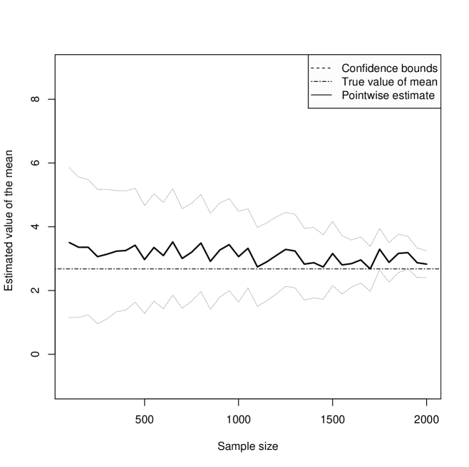
Figure 3.3: Confidence intervals for the mean $\mu$ based on $200$ samples of size $n,$ ranging from $100$ to $2000,$ from a Fréchet population with shape parameter $\alpha=1.5.$ The horizontal line represents the true value $\mu=2.678.$

Our simulation study, which is based on $200$ samples of various sizes from the Fréchet distribution (2.22) with two distinct tail index values $\alpha=1.5$ and $1.7,$ consists of three parts. First, we compare, in terms of bias and root of the mean squared error (RMSE), the performances of the new estimator $\widehat{\mu}_{n}$ and Peng’s estimator $\widehat{\mu}_{n}^{P}.$ The results of this part are summarized in Tables 3.1 and 3.2. Second, we check the asymptotic normality of both estimators via four of the most popular goodness-of-fit tests at the $5\%$ significance level: Cramér-von Mises (CvM), Kolmogrov-Smirnov (KS), Shapiro-Wilk (SW) and Pearson (P). The results of this part are summarized in Tables 3.3 and 3.4 and illustrated by Figures 3.1 and 3.2. Finally, we investigate the accuracy of the confidence intervals, built from the new estimator $\widehat{\mu}_{n},$ by computing their lengths and coverage probabilities (denoted by ‘covpr’). The results of this part are summarized in Table 3.5 (where ‘lcb’ and ‘ucb’ respectively stand for the lower and upper confidence bounds) and illustrated by Figure 3.3.

	$\widehat{\mu}_{n}$				$\widehat{\mu}_{n}^{P}$
Sample size	${\small 500}$	${\small 1000}$	${\small 2000}$	${\small 3000}$	${\small 500}$	${\small 1000}$	${\small 2000}$	${\small 3000}$
Estimated value	${\small 3.089}$	${\small 2.999}$	${\small 2.912}$	${\small 2.467}$	${\small 3.367}$	${\small 3.119}$	${\small 3.119}$	${\small 2.289}$
Bias	${\small 0.411}$	${\small 0.321}$	${\small 0.234}$	${\small 0.204}$	${\small 0.689}$	${\small 0.441}$	${\small 0.441}$	${\small 0.389}$
RMSE	${\small 0.400}$	${\small 0.286}$	${\small 0.125}$	${\small 0.108}$	${\small 0.674}$	${\small 0.268}$	${\small 0.268}$	${\small 0.198}$

Table 3.1: Point estimation of the mean based on 200 samples from the Fréchet population with shape parameter $\alpha=1.5$. The true value of the mean is 2.678.

	$\widehat{\mu}_{n}$				$\widehat{\mu}_{n}^{P}$
Sample size	${\small 500}$	${\small 1000}$	${\small 2000}$	${\small 3000}$	${\small 500}$	${\small 1000}$	${\small 2000}$	${\small 3000}$
Estimated value	${\small 2.536}$	${\small 2.440}$	${\small 2.354}$	${\small 2.254}$	${\small 2.765}$	${\small 2.731}$	${\small 2.566}$	${\small 2.460}$
Bias	${\small 0.383}$	${\small 0.287}$	${\small 0.201}$	${\small 0.101}$	${\small 0.612}$	${\small 0.578}$	${\small 0.413}$	${\small 0.307}$
RMSE	${\small 0.340}$	${\small 0.211}$	${\small 0.114}$	${\small 0.089}$	${\small 0.659}$	${\small 0.420}$	${\small 0.250}$	${\small 0.144}$

Table 3.2: Point estimation of the mean based on 200 samples from the Fréchet population with shape parameter $\alpha=1.7$. The true value of the mean is 2.153.

Sample size	CvM	KS	SW	P
${\small 100}$	${\small 0.447}$	${\small 0.401}$	${\small 0.198}$	${\small 0.165}$
${\small 200}$	${\small 0.729}$	${\small 0.626}$	${\small 0.795}$	${\small 0.549}$
${\small 400}$	${\small 0.267}$	${\small 0.256}$	${\small 0.347}$	${\small 0.331}$
${\small 500}$	${\small 0.306}$	${\small 0.354}$	${\small 0.410}$	${\small 0.302}$
${\small 800}$	${\small 0.374}$	${\small 0.396}$	${\small 0.412}$	${\small 0.486}$
${\small 1000}$	${\small 0.738}$	${\small 0.706}$	${\small 0.691}$	${\small 0.722}$

Sample size	CvM	KS	SW	P
${\small 100}$	${\small 0.001}$	${\small 0.000}$	${\small 0.000}$	${\small 0.002}$
${\small 200}$	${\small 0.009}$	${\small 0.006}$	${\small 0.024}$	${\small 0.104}$
${\small 400}$	${\small 0.495}$	${\small 0.446}$	${\small 0.377}$	${\small 0.500}$
${\small 500}$	${\small 0.209}$	${\small 0.273}$	${\small 0.158}$	${\small 0.329}$
${\small 800}$	${\small 0.419}$	${\small 0.321}$	${\small 0.378}$	${\small 0.344}$
${\small 1000}$	${\small 0.724}$	${\small 0.711}$	${\small 0.590}$	${\small 0.733}$

Table 3.3: Empirical p-values of normality tests for the new estimator (left panel) and Peng’s estimator (right panel) based on 200 samples from a Fréchet population with shape parameter $\alpha=1.5$.

Sample size	CvM	KS	SW	P
${\small 100}$	${\small 0.153}$	${\small 0.076}$	${\small 0.107}$	${\small 0.364}$
${\small 200}$	${\small 0.220}$	${\small 0.143}$	${\small 0.288}$	${\small 0.249}$
${\small 400}$	${\small 0.511}$	${\small 0.515}$	${\small 0.397}$	${\small 0.524}$
${\small 500}$	${\small 0.713}$	${\small 0.781}$	${\small 0.624}$	${\small 0.635}$
${\small 800}$	${\small 0.362}$	${\small 0.311}$	${\small 0.261}$	${\small 0.458}$
${\small 1000}$	${\small 0.778}$	${\small 0.783}$	${\small 0.645}$	${\small 0.601}$

Sample size	CvM	KS	SW	P
${\small 100}$	${\small 0.013}$	${\small 0.014}$	${\small 0.004}$	${\small 0.010}$
${\small 200}$	${\small 0.278}$	${\small 0.260}$	${\small 0.248}$	${\small 0.216}$
${\small 400}$	${\small 0.392}$	${\small 0.380}$	${\small 0.298}$	${\small 0.349}$
${\small 500}$	${\small 0.520}$	${\small 0.492}$	${\small 0.480}$	${\small 0.528}$
${\small 800}$	${\small 0.619}$	${\small 0.665}$	${\small 0.408}$	${\small 0.518}$
${\small 1000}$	${\small 0.720}$	${\small 0.688}$	${\small 0.485}$	${\small 0.567}$

Table 3.4: Empirical p-values of normality tests for the new estimator (left panel) and Peng’s estimator (right panel) based on 200 samples from a Fréchet population with shape parameter $\alpha=1.7$.

${\small n}$	lcb	$\widehat{\mu}$	ucb	covpr	length	${\small n}$	lcb	$\widehat{\mu}$	ucb	covpr	length
${\small 100}$	${\small-0.239}$	${\small 2.992}$	${\small 3.793}$	${\small 0.666}$	${\small 4.032}$	${\small 100}$	${\small-0.524}$	${\small 2.823}$	${\small 3.281}$	${\small 0.566}$	${\small 3.805}$
${\small 200}$	${\small 0.971}$	${\small 3.071}$	${\small 3.623}$	${\small 0.445}$	${\small 2.652}$	${\small 200}$	${\small-0.283}$	${\small 2.794}$	${\small 3.257}$	${\small 0.681}$	${\small 3.540}$
${\small 400}$	${\small 1.485}$	${\small 3.061}$	${\small 3.602}$	${\small 0.603}$	${\small 2.117}$	${\small 400}$	${\small 0.760}$	${\small 2.766}$	${\small 3.197}$	${\small 0.700}$	${\small 2.437}$
${\small 500}$	${\small 1.497}$	${\small 3.026}$	${\small 3.565}$	${\small 0.666}$	${\small 2.068}$	${\small 500}$	${\small 0.770}$	${\small 2.544}$	${\small 3.154}$	${\small 0.733}$	${\small 2.384}$
${\small 800}$	${\small 1.708}$	${\small 2.943}$	${\small 3.403}$	${\small 0.785}$	${\small 1.695}$	${\small 800}$	${\small 0.712}$	${\small 2.471}$	${\small 3.013}$	${\small 0.800}$	${\small 2.301}$
${\small 1000}$	${\small 1.922}$	${\small 2.883}$	${\small 3.302}$	${\small 0.795}$	${\small 1.380}$	${\small 1000}$	${\small 1.061}$	${\small 2.451}$	${\small 2.492}$	${\small 0.833}$	${\small 1.431}$

Table 3.5: Accuracy of $95\%$ confidence intervals for the new estimator based on 200 samples from Fréchet populations with shape parameters $\alpha=1.5$ (left panel) and $\alpha=1.7$ (right panel).

.

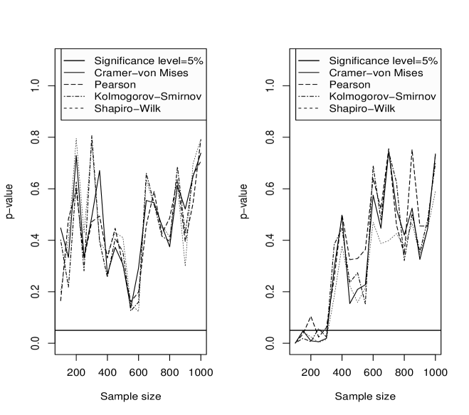
Figure 3.1: Empirical p-values of normality tests for the new estimator (left panel) and Peng’s estimator (right panel) based on $200$ samples of a Fréchet population with shape parameter $\alpha=1.5.$

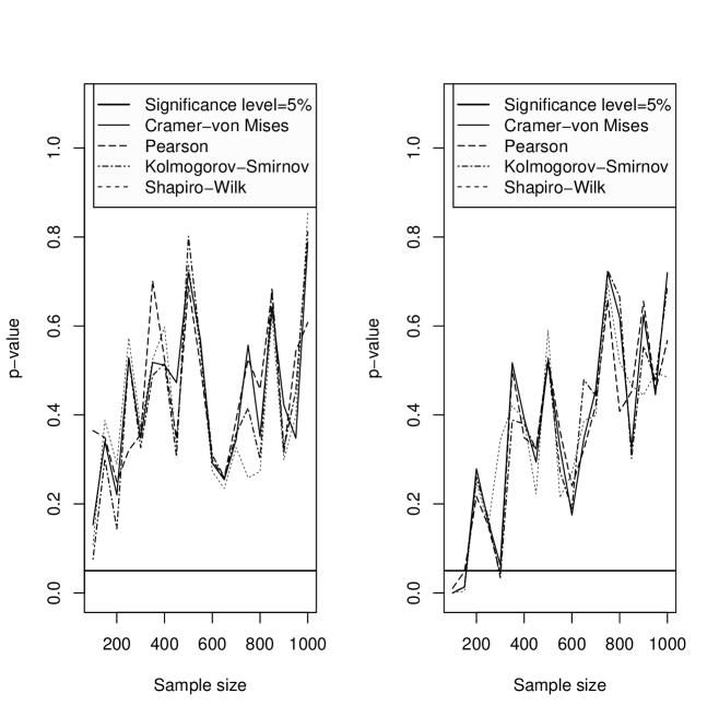
Figure 3.2: Empirical p-values of normality tests for the new estimator (left panel) and Peng’s estimator (right panel) based on $200$ samples from a Fréchet population with shape parameter $\alpha=1.7.$

Tables 3.1 and 3.2 show that, regardless of the sample size, our new estimator performs better than Peng’s one as far as the bias and RMSE are concerned. Moreover, from the left panels of Figure 3.2 and Table 3.4 (corresponding to the case of the lighter tail $\alpha=1.7)$ we see that the normality of $\widehat{\mu}_{n}$ cannot be rejected by any of the tests when the sample size exceeds $100,$ while the right panels of Figure 3.2 and Table 3.4 show that the normality of $\widehat{\mu}_{n}^{P}$ is rejected for sample sizes ranging between $100$ and $200.$ In the case of the heavier tail $\alpha=1.5,$ the right panels of Figure 3.1 and Table 3.3 show that the sample size needs to be larger then $400$ for the estimator $\widehat{\mu}_{n}^{P}$ to pass the normality tests, while the left panels of Figure 3.1 and Table 3.3 indicate that the normality of $\widehat{\mu}_{n}$ is accepted even for sample sizes smaller than $200.$

4 Proofs

4.1 Proof of Theorem 2.1.

First recall that $\lambda=\beta/\alpha>1.\$Then, from expansion $\left(4.1\right)$ in [Li et al. (2010)], we have, as $n\rightarrow\infty$

$$\widehat{\alpha}-\alpha=\alpha\left\{\eta_{1}\left(S_{1}-1\right)+\eta_{2}\left(S_{2}-\lambda^{-1}\right)+\eta_{3}\left(S_{3}-\lambda^{-2}\right)\right\}+o_{p}\left(k^{-1/2}\right),$$ (4.26)

where

$$S_{1}:=\dfrac{1}{k}{\displaystyle\sum\limits_{i=1}^{k}}\log\dfrac{Y_{n-i+1,n}}{Y_{n-k,n}},\text{ }S_{2}:=\dfrac{1}{k}{\displaystyle\sum\limits_{i=1}^{k}}\left(\dfrac{Y_{n-i+1,n}}{Y_{n-k,n}}\right)^{1-\lambda},$$ (4.27)

and

$$S_{3}:=\dfrac{1}{k}\sum\limits_{i=1}^{k}\left(\dfrac{Y_{n-i+1,n}}{Y_{n-k,n}}\right)^{1-\lambda}\log\dfrac{Y_{n-i+1,n}}{Y_{n-k},_{n}},$$ (4.28)

with $Y_{1,n}\leq...\leq Y_{n,n}$ being the order statistics pertaining to a sample $Y_{1},...,Y_{n}$ of i.i.d. r.v.’s, defined on the same probability space as the $X_{i}^{\prime}s,$ with cdf

$$G\left(y\right)=1-y^{-1},\text{ for }y>1.$$ (4.29)

[Csörgő et al. (1986)] have constructed a probability space $\left(\Omega,\emph{A,}\mathbf{P}\right)$ carrying an infinite sequence $U_{1},U_{2},...$ of independent $\left(0,1\right)-$uniform r.v.’s and a sequence of Brownian bridges $\left\{B_{n}\left(s\right),\text{ }0\leq s\leq 1\right\},$ $n=1,2,...,$ having, amongst others, the property stated in Lemma 4.1. Let $U_{1,n}\leq...\leq U_{n,n}$ denote the order statistics pertaining to $U_{1},...,U_{n}$ and define the empirical quantile function $V_{n}\left(s\right)$ as

$$V_{n}\left(s\right)=U_{i,n}\quad\text{for}\ \left(i-1\right)/n<s\leq i/n,\text{ }i=1,...,n,\text{ and }V_{n}\left(0\right)=U_{1,n}.$$

Lemma 4.1

On the probability space of [Csörgő et al. (1986)], for every $0\leq\tau<1/2,$ we have, as $n\rightarrow\infty$

$$\sup_{1/n\leq s\leq 1-1/n}\frac{\left|\sqrt{n}\left(s-V_{n}\left(s\right)\right)-B_{n}\left(s\right)\right|}{\left(s\left(1-s\right)\right)^{1/2-\tau}}=O_{p}\left(n^{-\tau}\right).$$ (4.30)

Proof. See the proof of Theorem 2.1 in [Csörgő et al. (1986)]. $\square$

Without loss of generality, we assume that

$$Y_{i}=G^{-1}\left(U_{i}\right)=\left(1-U_{i}\right)^{-1},\text{ }i=1,...,n,$$

and

$$Y_{i,n}=G^{-1}\left(U_{i,n}\right)=\left(1-U_{i,n}\right)^{-1},\text{ }i=1,...,n,$$

where $G^{-1}$ denotes the quantile function pertaining to cdf $G$ given by formula (4.29).  Then, this allows us to write

$$Y_{n-i+1,n}=\left(1-V_{n}\left(1-s\right)\right)^{-1},\text{ for }\dfrac{i-1}{n}<s\leq\dfrac{i}{n},\text{ }i=1,...,n.$$

Making use of the previous representation of the order statistics $Y_{n-i+1,n}$, we may rewrite the three statistics in (4.27) and (4.28) into

$$S_{1} =\frac{n}{k}\int_{0}^{k/n}\log\left(\frac{1-V_{n}\left(1-s\right)}{1-U_{n-k,n}}\right)^{-1}ds,$$

$$S_{2} =\frac{n}{k}\int_{0}^{k/n}\left(\frac{1-V_{n}\left(1-s\right)}{1-U_{n-k,n}}\right)^{-1+\lambda}ds,$$

and

$$S_{3}=\frac{n}{k}\int_{0}^{k/n}\left(\frac{1-V_{n}\left(1-s\right)}{1-U_{n-k,n}}\right)^{-1+\lambda}\log\left(\frac{1-V_{n}\left(1-s\right)}{1-U_{n-k,n}}\right)^{-1}ds.$$

Next, we show that, as $n\rightarrow\infty$

$$\sqrt{k}\left(S_{1}-1\right) =W_{1n}+o_{p}\left(1\right),$$

$$\sqrt{k}\left(S_{2}-\lambda^{-1}\right) =W_{2n}+o_{p}\left(1\right),$$

and

$$\sqrt{k}\left(S_{3}-\lambda^{-2}\right)=W_{3n}+o_{p}\left(1\right),$$

where $W_{1n},W_{2n}$ and $W_{3n}$ are the Gaussian r.v.’s defined in Theorem 2.1.  We will only consider the asymptotic distribution of $S_{3}.$ The proofs for $S_{1}$ and $S_{2}$ use similar arguments. By letting $f\left(x\right)=x^{\lambda-1}\log x,$ the statistic $S_{3}$ becomes

$$S_{3}=-\left(n/k\right){\displaystyle\int_{0}^{k/n}}f\left(\dfrac{1-V_{n}\left(1-s\right)}{1-U_{n-k,n}}\right)ds.$$

An application of standard calculus gives $\int_{0}^{1}f\left(s\right)ds=-\lambda^{-2}.$ Therefore

$$S_{3}-\lambda^{-2}=-\left(n/k\right){\displaystyle\int_{0}^{k/n}}\left[f\left(\dfrac{1-V_{n}\left(1-s\right)}{1-U_{n-k,n}}\right)-f\left(\frac{s}{k/n}\right)\right]ds.$$

Let us follow similar techniques as those used in the proof of Lemma 9 in [Csörgő et al. (1985)]. We divide the integral above in two parts, then we study the asymptotic behavior of each integral. Observe that

$$S_{3}-\lambda^{-2} =-\left(n/k\right){\displaystyle\int_{0}^{1/n}}\left[f\left(\dfrac{1-V_{n}\left(1-s\right)}{1-U_{n-k,n}}\right)-f\left(\frac{s}{k/n}\right)\right]ds$$

$$\ \ \ \ \ \ \ -\left(n/k\right){\displaystyle\int_{1/n}^{k/n}}\left[f\left(\dfrac{1-V_{n}\left(1-s\right)}{1-U_{n-k,n}}\right)-f\left(\frac{s}{k/n}\right)\right]ds$$

$$\begin{array}[c]{c}=:\end{array}-\Delta_{n}-\Omega_{n}.$$

Next, we show that $\sqrt{k}\Delta_{n}$ converges to $0$ in probability. Indeed, we have $1-V_{n}\left(1-s\right)=1-U_{n,n},$ for $0<s\leq 1/n,$ it follows that

$$\Delta_{n} =\left(n/k\right){\displaystyle\int_{0}^{1/n}}\left[f\left(\dfrac{1-U_{n,n}}{1-U_{n-k,n}}\right)-f\left(\frac{s}{k/n}\right)\right]ds$$

$$=k^{-1}f\left(\dfrac{1-U_{n,n}}{1-U_{n-k,n}}\right)-{\displaystyle\int_{0}^{1/k}}f\left(s\right)ds.$$

An elementary calculation gives ${\displaystyle\int_{0}^{1/k}}f\left(s\right)ds=\lambda^{-1}k^{-\lambda}\left(\log k^{-1}-\lambda^{-1}\right),$ and from Lemma 2.2.3 of page 41 in [de Haan and Ferreria, (2006)], we have $n\left(1-U_{n,n-k}\right)/k\overset{P}{\rightarrow}1,$ as $n\rightarrow\infty,$ therefore

$$\Delta_{n}=\left\{1+o_{p}\left(1\right)\right\}k^{-\lambda}\log k^{-1}-\lambda^{-1}k^{-\lambda}\left(\log k^{-1}-\lambda^{-1}\right).$$

Since $\lambda>1$ and $k\rightarrow\infty,$ then $k^{-\lambda+1/2}\rightarrow 0$ and $k^{-\lambda+1/2}\log k^{-1}\rightarrow 0,$ it follows that $\sqrt{k}\Delta_{n}\overset{P}{\rightarrow}0$ as $n\rightarrow\infty.$ Consider now the second term $\Omega_{n}$ which may be rewritten into

$$\Omega_{n} =\left(n/k\right){\displaystyle\int_{1/n}^{k/n}}\left[f\left(\dfrac{1-V_{n}\left(1-s\right)}{1-U_{n-k,n}}\right)-f\left(\dfrac{s}{1-U_{n-k,n}}\right)\right]ds$$

$$\ \ \ \ \ \ \ \ \ \ \ \ \ \ \ \ \ +\left(n/k\right){\displaystyle\int_{1/n}^{k/n}}\left[f\left(\dfrac{s}{1-U_{n-k,n}}\right)-f\left(\dfrac{s}{k/n}\right)\right]ds$$

$$\begin{array}[c]{c}=:\end{array}\Omega_{n1}+\Omega_{n2}.$$

Making use of Taylor’s expansion of $f,$ we get

$$f\left(\dfrac{1-V_{n}\left(1-s\right)}{1-U_{n-k,n}}\right)-f\left(\dfrac{s}{1-U_{n-k,n}}\right)=f^{\prime}\left(\frac{\varphi_{n}\left(s\right)}{1-U_{n-k,n}}\right)\left(\dfrac{1-V_{n}\left(1-s\right)}{1-U_{n-k,n}}-\dfrac{s}{1-U_{n-k,n}}\right),$$

and

$$f\left(\dfrac{s}{1-U_{n-k,n}}\right)-f\left(\dfrac{s}{k/n}\right)=f^{\prime}\left(s\psi_{n}\right)\left(\dfrac{s}{1-U_{n-k,n}}-\dfrac{s}{k/n}\right),$$

where

$$\min\left\{1-V_{n}\left(1-s\right),s\right\}<\varphi_{n}\left(s\right)<\max\left\{1-V_{n}\left(1-s\right),s\right\}$$ (4.31)

and

$$\min\left\{\dfrac{1}{1-U_{n-k,n}},\dfrac{1}{k/n}\right\}<\psi_{n}<\max\left\{\dfrac{1}{1-U_{n-k,n}},\dfrac{1}{k/n}\right\}.$$ (4.32)

Observe now that $\Omega_{n1}$ and $\Omega_{n2}$ may be rewritten into

$$\Omega_{n1}=\left(n/k\right){\displaystyle\int_{1/n}^{k/n}}f^{\prime}\left(\dfrac{s}{1-U_{n-k,n}}\right)\left[\dfrac{1-V_{n}\left(1-s\right)}{1-U_{n-k,n}}-\dfrac{s}{1-U_{n-k,n}}\right]ds+\Omega_{n1}^{\ast},$$

and

$$\Omega_{n2}=\left\{1+o_{p}\left(1\right)\right\}\left(n/k\right){\displaystyle\int_{1/n}^{k/n}}f^{\prime}\left(\dfrac{s}{k/n}\right)\left[\dfrac{s}{1-U_{n-k,n}}-\dfrac{s}{k/n}\right]ds+\Omega_{n2}^{\ast},$$

where

$$\Omega_{n1}^{\ast}\begin{array}[c]{c}:=\end{array}\left(n/k\right){\displaystyle\int_{1/n}^{k/n}}\left[f^{\prime}\left(\dfrac{\varphi_{n}\left(s\right)}{1-U_{n-k,n}}\right)-f^{\prime}\left(\dfrac{s}{1-U_{n-k,n}}\right)\right]$$

$$\ \ \ \ \ \ \ \ \ \ \ \ \ \ \ \ \ \ \ \ \ \ \ \ \ \ \ \ \ \ \ \ \ \ \ \ \ \ \ \ \ \times\left[\dfrac{1-V_{n}\left(1-s\right)}{1-U_{n-k,n}}-\dfrac{s}{1-U_{n-k,n}}\right]ds,$$

and

$$\Omega_{n2}^{\ast}\begin{array}[c]{c}:=\end{array}\left\{1+o_{p}\left(1\right)\right\}\left(n/k\right){\displaystyle\int_{1/n}^{k/n}}\left[f^{\prime}\left(\dfrac{s\psi_{n}}{k/n}\right)-f^{\prime}\left(\dfrac{s}{k/n}\right)\right]$$

$$\ \ \ \ \ \ \ \ \ \ \ \ \ \ \ \ \ \ \ \ \ \ \ \ \ \ \ \ \ \ \ \ \ \ \ \ \ \ \ \ \ \ \ \ \ \ \ \ \times\left[\dfrac{s}{1-U_{n-k,n}}-\dfrac{s}{k/n}\right]ds.$$

From Lemma A.2 (see the Appendix), both $\sqrt{k}\Omega_{n1}^{\ast}$ and $\sqrt{k}\Omega_{n2}^{\ast}$ converge to $0$ in probability. Since $n\left(1-U_{n-k,n}\right)/k\overset{P}{\rightarrow}1,$ then

$$\Omega_{n1}=\left\{1+o_{p}\left(1\right)\right\}{\displaystyle\int_{1/n}^{k/n}}f^{\prime}\left(\dfrac{s}{k/n}\right)\left[1-s-V_{n}\left(1-s\right)\right]ds+o_{p}\left(k^{-1/2}\right),$$

and

$$\Omega_{n2}=-\left\{1+o_{p}\left(1\right)\right\}\dfrac{k/n-\left(1-U_{n-k,n}\right)}{\left(k/n\right)^{2}}{\displaystyle\int_{1/n}^{k/n}}\left(\dfrac{s}{k/n}\right)f^{\prime}\left(\dfrac{s}{k/n}\right)ds+o_{p}\left(k^{-1/2}\right).$$

The derivative of function $f$ equals $f^{\prime}\left(x\right)=(\lambda-1)x^{\lambda-2}\log x+x^{\lambda-2},$ then

$$\Omega_{n1} =\left(\lambda-1\right)\left(n/k\right){\displaystyle\int_{1/k}^{1}}t^{\lambda-2}\left(\log t\right)\left[1-V_{n}\left(1-kt/n\right)-kt/n\right]dt$$

$$\ \ \ \ \ \ \ \ \ \ \ \ \ \ \ \ \ \ \ \ \ \ \ \ \ \ +\left(n/k\right){\displaystyle\int_{1/k}^{1}}t^{\lambda-2}\left[1-V_{n}\left(1-kt/n\right)-kt/n\right]dt+o_{p}\left(k^{-1/2}\right),$$

and

$$\Omega_{n2} =\left(\lambda-1\right)\left(n/k\right)\left[k/n-\left(1-U_{n-k,n}\right)\right]{\displaystyle\int_{1/k}^{1}}t^{\lambda-1}\log tdt$$

$$\ \ \ \ \ \ \ \ \ \ \ \ \ \ \ \ \ \ +\left(n/k\right)\left[k/n-\left(1-U_{n-k,n}\right)\right]{\displaystyle\int_{1/k}^{1}}t^{\lambda-1}dt+o_{p}\left(k^{-1/2}\right)$$

$$=\lambda^{-2}\left(n/k\right)\left[k/n-\left(1-U_{n-k,n}\right)\right]+o_{p}\left(k^{-1/2}\right).$$

Fix $0<\tau<1/2,$ then using approximation (4.30), in Lemma 4.1, yields

$$\sqrt{k}\Omega_{n1} =\left(\lambda-1\right)\sqrt{n/k}{\displaystyle\int_{1/k}^{1}}t^{\lambda-2}\left(\log t\right)B_{n}\left(1-kt/n\right)dt$$

$$\ \ \ \ \ \ \ +\sqrt{n/k}{\displaystyle\int_{1/k}^{1}}t^{\lambda-2}B_{n}\left(1-kt/n\right)dt+\sqrt{k}\widetilde{\Omega}_{n1}\left(\tau\right)+o_{p}\left(1\right),$$

and

$$\sqrt{k}\Omega_{n2}=-\lambda^{-2}\sqrt{n/k}B_{n}\left(1-k/n\right)+\sqrt{k}\widetilde{\Omega}_{n2}\left(\tau\right)+o_{p}\left(1\right),$$

where

$$\sqrt{k}\widetilde{\Omega}_{n1}\left(\tau\right) =\left(\lambda-1\right)O_{p}\left(n^{-\tau}\right)\left(k/n\right)^{1/2-\tau}\left(n/k\right)^{1/2}{\displaystyle\int_{0}^{1}}t^{\lambda-2+\left(1/2-\tau\right)}\left|\log t\right|dt$$

$$\ \ \ \ \ \ \ \ \ \ \ \ \ \ \ \ \ \ \ \ \ \ \ \ \ \ \ \ \ +O_{p}\left(n^{-\tau}\right)\left(k/n\right)^{1/2-\tau}\sqrt{n/k}{\displaystyle\int_{0}^{1}}t^{\lambda-2+\left(1/2-\tau\right)}dt,$$

and

$$\sqrt{k}\widetilde{\Omega}_{n2}\left(\tau\right)=\lambda^{-2}O_{p}\left(n^{-\tau}\right)\sqrt{n/k}\left(k/n\right)^{1/2-\tau}.$$

For $\lambda>1,$ ${\displaystyle\int_{0}^{1}}t^{\lambda-2+\left(1/2-\tau\right)}\left|\log t\right|dt=\left(\lambda-1/2-\tau\right)^{-2}$ and ${\displaystyle\int_{0}^{1}}t^{\lambda-2+\left(1/2-\tau\right)}dt=\left(\lambda-1/2-\tau\right)^{-1}$ are finite integrals. Then both quantities $\sqrt{k}\widetilde{\Omega}_{n1}$ and $\sqrt{k}\widetilde{\Omega}_{n2}$ are equal to $O_{p}\left(k^{-\tau}\right)$ for all large $n,$ which tends in probability to $0$ as $n\rightarrow\infty.$ Recall that up to now we have showed that

$$\sqrt{k}\Omega_{n1} =\left(\lambda-1\right)\sqrt{n/k}{\displaystyle\int_{1/k}^{1}}t^{\lambda-2}\left(\log t\right)B_{n}\left(1-kt/n\right)dt$$

$$\ \ \ \ \ \ \ \ \ \ \ \ \ \ \ \ \ \ \ \ \ \ \ \ +\sqrt{n/k}{\displaystyle\int_{1/k}^{1}}t^{\lambda-2}B_{n}\left(1-kt/n\right)dt+o_{p}\left(1\right),$$

and

$$\sqrt{k}\Omega_{n2}=\lambda^{-2}\sqrt{n/k}B_{n}\left(1-k/n\right)+o_{p}\left(1\right).$$

It remains to prove that

$$I_{n}\begin{array}[c]{c}:=\end{array}\left(\lambda-1\right)\sqrt{n/k}{\displaystyle\int_{0}^{1/k}}t^{\lambda-2}\left(\log t\right)B_{n}\left(1-kt/n\right)dt$$

$$\ \ \ \ \ \ \ \ \ \ \ \ \ \ \ \ \ \ \ \ \ \ \ \ \ \ \ \ \ \ \ \ \ \ \ \ \ \ +\sqrt{n/k}{\displaystyle\int_{0}^{1/k}}t^{\lambda-2}B_{n}\left(1-kt/n\right)dt,$$

converges, in probability, to $0.$ Indeed, since $E\left|B_{n}\left(1-ks/n\right)\right|\leq\sqrt{ks/n},$ then

$$\mathbf{E}\left|I_{n}\right|\leq\left(\lambda-1\right){\displaystyle\int_{0}^{1/k}}t^{\lambda-2+1/2}\left(\left|\log t\right|+1\right)dt.$$

Since

$${\displaystyle\int_{0}^{1/k}}t^{\lambda-2+1/2}\left(\left|\log t\right|+1\right)dt=\frac{2}{\left(2\lambda-1\right)^{2}}k^{-\lambda+\frac{1}{2}}\left(2\lambda-\log k+2\lambda\log k+1\right),$$

which tends to $0$ as $n\rightarrow\infty,$ then $I_{n}$ converges to $0$ in probability. This completes the proof of Theorem 2.1. $\square$

4.2 Proof of Theorem 2.2.

To establish the asymptotic normality of $\widehat{\alpha}$, given in $\left(\ref{asympt-alpha}\right),$ we proceed by similar arguments as for $\widehat{\mu}_{n}$ in the proof of Theorem 2.4. $\square$

4.3 Proof of Theorem 2.3

Let us divide the integral (1.2), in two parts, as follows:

$$\mu=\mu_{1,n}\left(k\right)+\mu_{2,n}\left(k\right),$$

where

$$\mu_{1,n}\left(k\right):=\int_{0}^{k/n}Q\left(1-s\right)ds\text{ and }\mu_{2,n}\left(k\right):=\int_{k/n}^{1}Q\left(1-s\right)ds.$$

Recall that, in Section 1 formula (1.16), we have defined estimator $\widehat{\mu}_{n}$ of $\mu$ by

$$\widehat{\mu}_{n}=\widehat{\mu}_{1,n}\left(k\right)+\widehat{\mu}_{2,n}\left(k\right),$$

where

$$\widehat{\mu}_{1,n}\left(k\right):=\left(k/n\right)\left(n\widehat{c}/k\right)^{1/\widehat{\alpha}}\left\{\frac{\widehat{\alpha}}{\widehat{\alpha}-1}+\frac{\widehat{d}\widehat{c}^{-\widehat{\beta}/\widehat{\alpha}}\left(k/n\right)^{\widehat{\beta}/\widehat{\alpha}-1}}{\widehat{\beta}-1}\right\}$$

and

$$\widehat{\mu}_{2,n}\left(k\right):=\frac{1}{n}\sum_{i=k+1}^{n}X_{n-i+1,n}.$$

To simplify notations, let us set

$$Z_{ni}:=\frac{\sqrt{n}}{\sqrt{k/n}\left(nc/k\right)^{1/\alpha}}\left\{\widehat{\mu}_{i,n}\left(k\right)-\mu_{i,n}\left(k\right)\right\},\text{ }i=1,2.$$ (4.33)

First, we consider $Z_{n1}.$ It is easy to verify that, as $n\rightarrow\infty$

$$\mu_{1,n}\left(k\right)=\left\{1+o_{p}\left(1\right)\right\}\frac{k}{n}\left(nc/k\right)^{1/\alpha}\frac{\alpha}{\alpha-1},$$

and, under the condition (1.6), we have

$$\widehat{\mu}_{1,n}\left(k\right)=\left\{1+o_{p}\left(1\right)\right\}\frac{k}{n}\frac{\widehat{\alpha}}{\widehat{\alpha}-1}\left(n\widehat{c}/k\right)^{1/\widehat{\alpha}}.$$

It follows that

$$\widehat{\mu}_{1,n}\left(k\right)-\mu_{1,n}\left(k\right)=\left\{1+o_{p}\left(1\right)\right\}\frac{k}{n}\left\{\frac{\widehat{\alpha}}{\widehat{\alpha}-1}\left(n\widehat{c}/k\right)^{1/\widehat{\alpha}}-\frac{\alpha}{\alpha-1}\left(nc/k\right)^{1/\alpha}\right\}.$$

Let us write $Z_{n1}=T_{1n}+T_{2n},$ where

$$T_{1n}:=\left\{1+o_{p}\left(1\right)\right\}\sqrt{k}\left\{\frac{\widehat{\alpha}}{\widehat{\alpha}-1}-\frac{\alpha}{\alpha-1}\right\},$$

and

$$T_{2n}:=\left\{1+o_{p}\left(1\right)\right\}\sqrt{k}\left\{\frac{\left(n\widehat{c}/k\right)^{1/\widehat{\alpha}}}{\left(nc/k\right)^{1/\alpha}}-1\right\}.$$

We begin by showing that $T_{2n}\overset{P}{\rightarrow}0,$ as $n\rightarrow\infty.$ First observe that $T_{2n}$ may be rewritten into

$$T_{2n}=\left\{1+o_{p}\left(1\right)\right\}\sqrt{k}\left\{\left(nc/k\right)^{1/\widehat{\alpha}-1/\alpha}\left(\widehat{c}/c\right)^{1/\widehat{\alpha}-1/\alpha}-1\right\}.$$

Assumptions $\left(i\right)$ and $\left(ii\right)$ of Theorem 2.1 imply that $k^{1/2}/\log\left(n/k\right)\rightarrow\infty.\$Also, from Theorem 1 of [Peng and Qi, (2004)], the asymptotic normality of $\widehat{\alpha}$ gives $\widehat{\alpha}-\alpha=O_{p}\left(k^{-1/2}\right).$ Therefore $\left(1/\widehat{\alpha}-1/\alpha\right)\log\left(nc/k\right)\overset{P}{\rightarrow}0,$ this implies that $\left(nc/k\right)^{1/\widehat{\alpha}-1/\alpha}\overset{P}{\rightarrow}1,$ as $n\rightarrow\infty.$ On the other hand, from equation $\left(4.7\right)$ in [Li et al. (2010)], we have

$$\widehat{c}/c-1=\alpha^{-1}\left(\widehat{\alpha}-\alpha\right)\log\dfrac{n}{k}+o_{p}\left(k^{-1/2}\log\dfrac{n}{k}\right).$$

Since $\widehat{c}$ is a consistent estimator of $c,$ then Taylor’s expansion gives

$$\left(\widehat{c}/c\right)^{1/\widehat{\alpha}-1/\alpha}-1=\alpha^{-1}\left(1+o_{p}\left(1\right)\right)\left(\widehat{\alpha}-\alpha\right)\left(\widehat{c}/c-1\right),\text{ as }n\rightarrow\infty.$$

It suffices now to show that $\sqrt{k}\left(\left(\widehat{c}/c\right)^{1/\widehat{\alpha}-1/\alpha}-1\right)$ converges to $0$ in probability.  Indeed, again by using the fact that $\widehat{\alpha}-\alpha=O_{p}\left(k^{-1/2}\right),$ yields

$$\sqrt{k}\left(\left(\widehat{c}/c\right)^{1/\widehat{\alpha}-1/\alpha}-1\right)=O_{p}\left(1\right)\left(k^{-1/2}\log\dfrac{n}{k}+o_{p}\left(\frac{\log\dfrac{n}{k}}{\sqrt{k}}\right)\right),$$

which tends in probability to $0,$ because we already have $\sqrt{k}/\log\left(n/k\right)\rightarrow\infty.$ Now, we consider the term $T_{1n}.$ Since $\widehat{\alpha}$ is a consistent estimator of $\alpha,$ then it is easy to show that

$$T_{1n}=-\frac{1+o_{p}\left(1\right)}{\left(\alpha-1\right)^{2}}\sqrt{k}\left(\widehat{\alpha}-\alpha\right),\text{ as }n\rightarrow\infty.$$

From 2.1, we infer that

$$T_{1n}=-\frac{\left(1+o_{p}\left(1\right)\right)\alpha}{\left(\alpha-1\right)^{2}}\left(\eta_{1}W_{1n}+\eta_{2}W_{2n}+\eta_{3}W_{3n}\right),\text{ as }n\rightarrow\infty.$$

It follows that

$$Z_{n1}=-\frac{\alpha}{\left(\alpha-1\right)^{2}}\left\{\eta_{1}W_{1n}+\eta_{2}W_{2n}+\eta_{3}W_{3n}\right\}+o_{p}\left(1\right).$$ (4.34)

Let us now consider the asymptotic distribution of $Z_{n2},$ in (4.33). It is shown in [Csörgő and Mason, (1985)] or more recently in [Necir and Meraghni, (2009)] that

$$Z_{n2}=-\frac{\int_{k/n}^{1}B_{n}\left(1-s\right)dQ\left(1-s\right)}{\sqrt{k/n}Q\left(1-k/n\right)}+o_{p}\left(1\right).$$

On the other hand, from (1.10), we have $Q\left(1-k/n\right)\sim\left(nc/k\right)^{1/\alpha},$ as $n\rightarrow\infty,$ it follows that

$$Z_{n2}=W_{4n}+o_{p}\left(1\right).$$ (4.35)

Combining (4.34) and (4.35) achieves the proof of Theorem 2.3. $\square$

4.4 Proof of Theorem 2.4.

Now, we investigate the asymptotic normality of $\widehat{\mu}_{n}$ given in$\left(\ref{asympt-mu}\right)$. Since $W_{in},$ $i=1,...,4$ are sequences of centred Gaussian r.v.’s, then

$$\frac{\sqrt{n}}{\sqrt{k/n}\left(nc/k\right)^{1/\alpha}}\left\{\widehat{\mu}_{n}-\mu\right\}\overset{d}{\rightarrow}\mathcal{N}\left(0,\Gamma\Sigma\Gamma^{t}\right),\text{ as }n\rightarrow\infty,$$

where

$$\Gamma:=\left(-\frac{\alpha}{\left(\alpha-1\right)^{2}}\eta_{1},-\frac{\alpha}{\left(\alpha-1\right)^{2}}\eta_{2},-\frac{\alpha}{\left(\alpha-1\right)^{2}}\eta_{3},1\right),$$

$\Gamma^{t}$ is the transpose of $\Gamma$ and $\Sigma$ is the variance-covariance matrix of the vector $\left(W_{1n},...,W_{4n}\right)$ defined by

$$\sum=\left[\begin{array}[c]{cccc}1&\frac{1}{\lambda^{2}}-\frac{1}{\lambda}&\frac{2}{\lambda^{3}}-\frac{1}{\lambda^{2}}&-1\\ \frac{1}{\lambda^{2}}-\frac{1}{\lambda}&\frac{1}{2\lambda-1}-\frac{1}{\lambda^{2}}&\frac{1}{\left(2\lambda-1\right)^{2}}-\frac{1}{\lambda^{3}}&\frac{\lambda-1}{\lambda}\\ \frac{2}{\lambda^{3}}-\frac{1}{\lambda^{2}}&\frac{1}{\left(2\lambda-1\right)^{2}}-\frac{1}{\lambda^{3}}&\frac{2}{\left(2\lambda-1\right)^{3}}-\frac{1}{\lambda^{4}}&-\frac{1}{\lambda^{2}}\\ -1&\frac{\lambda-1}{\lambda}&-\frac{1}{\lambda^{2}}&\frac{2}{2-\alpha}\end{array}\right].$$

Note that the elements of $\sum$ were obtained after tedious computations of the limits of the expectations $\mathbf{E}\left[W_{in}W_{jn}\right]$ for $i,j=1,4$ $\left(i\leq j\right)$. Analogue calculus of these quantities may be found in [Peng, (2001)], [Necir and Meraghni, (2009)] and [Necir and Meraghni, (2010)]. Finally, a standard calculation of the product $\Gamma\Sigma\Gamma^{t}$ yields

$$\Gamma\Sigma\Gamma^{t}=\frac{\alpha^{2}\beta^{4}}{\left(\alpha-1\right)^{4}\left(\alpha-\beta\right)^{4}}+\frac{2}{2-\alpha}+\frac{2\alpha\beta^{2}}{\left(\alpha-1\right)^{2}\left(\alpha-\beta\right)^{2}},$$

which is denoted by $\sigma^{2}\left(\alpha,\beta\right).$ This completes the proof of Theorem 2.4. $\square$

5 Concluding notes

The main objective of this paper was to propose a bias-reduced estimator for the mean of a heavy-tailed distribution. This was achieved on the basis of the bias-reduction of the first and second order parameter estimators of regularly varying distributions developed by [Peng and Qi, (2004)] and the corresponding high quantiles estimators introduced by [Li et al. (2010)]. In addition, the newly introduced estimator is asymptotically normal, making confidence intervals easily constructible. We conclude by simulation that, compared to that of Peng, our new estimator has smaller bias and RMSE and consequently it performs better.

Appendix A Appendix

A.1 Auxiliary results

Lemma A.1

Let $k=k_{n}$ be a sequence of integers satisfying (1.6) and $f\left(x\right)=x^{\lambda-1}\log x,$ $\lambda>1.$ Then, uniformly on $s\in\left[1/n,k/n\right],$ we have

$$f^{\prime}\left(\dfrac{\varphi_{n}\left(s\right)}{1-U_{n-k,n}}\right)-f^{\prime}\left(\dfrac{s}{1-U_{n-k,n}}\right)=o_{p}\left(1\right)\left(\dfrac{s}{k/n}\right)^{\lambda-2}\log\dfrac{s}{k/n},\text{ as }n\rightarrow\infty.$$

Proof. We have $n\left(1-U_{n-k,n}\right)/k\overset{p}{\rightarrow}0,$ as $n\rightarrow\infty,$ then

$$f^{\prime}\left(\dfrac{\varphi_{n}\left(s\right)}{1-U_{n-k,n}}\right)-f^{\prime}\left(\dfrac{s}{1-U_{n-k,n}}\right)=\left(1+o_{p}\left(1\right)\right)\left[f^{\prime}\left(\dfrac{\varphi_{n}\left(s\right)}{k/n}\right)-f^{\prime}\left(\dfrac{s}{k/n}\right)\right].$$

A straightforward calculation of the derivative of $f$ yields

$$f^{\prime}\left(\dfrac{\varphi_{n}\left(s\right)}{k/n}\right)-f^{\prime}\left(\dfrac{s}{k/n}\right) =\left(\dfrac{s}{k/n}\right)^{\lambda-2}\left[\left(\lambda-1\right)\left(\left(\dfrac{\varphi_{n}\left(s\right)}{s}\right)^{\lambda-2}-1\right)\log\dfrac{\varphi_{n}\left(s\right)}{k/n}\right.$$

$$+\left.\left(\lambda-1\right)\log\dfrac{\varphi_{n}\left(s\right)}{s}+\left(\dfrac{\varphi_{n}\left(s\right)}{s}\right)^{\lambda-2}-1\right].$$ (1.36)

Observe now, that inequalities (4.31) imply

$$\min\left\{\frac{1-s-V_{n}\left(1-s\right)}{s},0\right\}<\dfrac{\varphi_{n}\left(s\right)}{s}-1<\max\left\{\frac{1-s-V_{n}\left(1-s\right)}{s},0\right\}.$$

From [Wellner, (1978)], we have

$$\sup_{1/n\leq s<1}\frac{\left|1-s-V_{n}\left(1-s\right)\right|}{s}\overset{p}{\rightarrow}0\text{ as }n\rightarrow\infty,$$

it follows that

$$\sup_{1/n\leq s\leq k/n}\left|\dfrac{\varphi_{n}\left(s\right)}{s}-1\right|\overset{p}{\rightarrow}0\text{ as }n\rightarrow\infty.$$ (1.37)

On the other hand, in view Lemma 3 in [Necir and Meraghni, (2009)], we infer that

$$\sup_{1/n\leq s\leq k/n}\left|\dfrac{s}{\varphi_{n}\left(s\right)}-1\right|\overset{p}{\rightarrow}0\text{ as }n\rightarrow\infty.$$ (1.38)

By applying the mean value theorem to the functions $x\rightarrow\log x$ and $x\rightarrow x^{\lambda-1}$ respectively, then by using (1.37) and (1.38), we show readily that, as $n\rightarrow\infty$

$$\sup_{1/n\leq s\leq k/n}\left|\log\dfrac{\varphi_{n}\left(s\right)}{s}\right|\overset{p}{\rightarrow}0\text{ and }\sup_{1/n\leq s\leq k/n}\left|\left(\dfrac{\varphi_{n}\left(s\right)}{s}\right)^{\lambda-1}-1\right|\overset{p}{\rightarrow}0.$$ (1.39)

Note that the first result of (1.39) implies that

$$\sup_{1/n\leq s\leq k/n}\left|\log\dfrac{\varphi_{n}\left(s\right)}{k/n}-\log\dfrac{s}{k/n}\right|\overset{p}{\rightarrow}0,\text{ as }n\rightarrow\infty.$$ (1.40)

By using equations (1.39) and (1.40) together, we show that, uniformly in $s\in\left[1/n,k/n\right],$ the right-hand side of equation $\left(\ref{eql}\right),$ is equal to $o_{p}\left(1\right)\left(\dfrac{s}{k/n}\right)^{\lambda-2}\log\dfrac{s}{k/n}.$ $\square$

Lemma A.2

We have $\sqrt{k}\Omega_{n1}^{\ast}\overset{p}{\rightarrow}0$ and $\sqrt{k}\Omega_{n2}^{\ast}\overset{p}{\rightarrow}0,$ as $n\rightarrow\infty.$

Proof. We only show the first result. The second one is obtained by similar arguments. Recall that

$$\Omega_{n1}^{\ast} :=-\left(n/k\right){\displaystyle\int_{1/n}^{k/n}}\left[f^{\prime}\left(\dfrac{\varphi_{n}\left(s\right)}{1-U_{n-k,n}}\right)-f^{\prime}\left(\dfrac{s}{1-U_{n-k,n}}\right)\right]$$

$$\ \ \ \ \ \ \ \ \ \ \ \ \ \ \ \ \ \ \ \ \ \ \ \ \ \ \ \ \ \ \ \times\left[\dfrac{1-V_{n}\left(1-s\right)}{1-U_{n-k,n}}-\dfrac{s}{1-U_{n-k,n}}\right]ds.$$

Using Lemma A.1, we get, as $n\rightarrow\infty$

$$\Omega_{n1}^{\ast}=o_{p}\left(1\right)\left(n/k\right){\displaystyle\int_{1/n}^{k/n}}\left(\dfrac{s}{k/n}\right)^{\lambda-2}\left|\log\dfrac{s}{k/n}\right|\left|\dfrac{1-V_{n}\left(1-s\right)}{k/n}-\dfrac{s}{k/n}\right|ds.$$

By a change of variables, we get

$$\Omega_{n1}^{\ast}=o_{p}\left(1\right)\left(n/k\right){\displaystyle\int_{1/k}^{1}}s^{\lambda-2}\left|\log s\right|\left|1-V_{n}\left(1-ks/n\right)-ks/n\right|ds.$$

Making use of approximation$\left(\ref{approxi}\right)$ yields

$$\sqrt{k}\Omega_{n1}^{\ast}=o_{p}\left(1\right)\left(n/k\right)^{1/2}{\displaystyle\int_{1/k}^{1}}s^{\lambda-2}\left|\log s\right|\left(\left|B_{n}\left(1-ks/n\right)\right|+\left(ks/n\right)^{1/2-\tau}O_{p}\left(n^{-\tau}\right)\right)ds.$$

In other words

$$\sqrt{k}\Omega_{n1}^{\ast} =o_{p}\left(1\right)\left(n/k\right)^{1/2}{\displaystyle\int_{1/k}^{1}}s^{\lambda-2}\left|\log s\right|\left|B_{n}\left(1-ks/n\right)\right|ds.$$

$$\ \ \ \ \ \ \ \ \ \ \ \ \ \ \ \ \ \ \ \ \ \ \ \ \ \ \ \ \ \ \ \ \ \ \ +o_{p}\left(k^{-\tau}\right){\displaystyle\int_{1/k}^{1}}s^{\lambda-3/2-\tau}\left|\log s\right|ds.$$

The expectation of the first term of right-hand side of the previous equation is less than or equal to

$$o_{p}\left(1\right)\left(n/k\right)^{1/2}{\displaystyle\int_{0}^{1}}s^{\lambda-2}\left|\log s\right|\mathbf{E}\left[\left|B_{n}\left(1-ks/n\right)\right|\right]ds.$$

Using the fact that $E\left|B_{n}\left(1-ks/n\right)\right|\leq\left(ks/n\right)^{1/2},$ we show that the previous quantity is less than or equal to $o_{p}\left(1\right){\displaystyle\int_{0}^{1}}s^{\lambda-3/2}\left|\log s\right|ds.$ Since both integrals ${\displaystyle\int_{0}^{1}}s^{\lambda-3/2-\tau}\left|\log s\right|ds$ and ${\displaystyle\int_{0}^{1}}s^{\lambda-3/2-\tau}\left|\log s\right|ds$ are finite, then $\sqrt{k}\Omega_{n1}^{\ast}=o_{p}\left(1\right),$ as $n\rightarrow\infty.\hfill\square$

A.2 Optimal choice of the sample fraction $k$

Reiss and Thomas in [Reiss and Thomas, (2007), , page 137], proposed a heuristic method for choosing the optimal number of upper extremes used in the computation of the tail index estimate. In this paper, we adopt this algorithm by making use of Peng and Qi estimator $\widehat{\alpha}=\widehat{\alpha}\left(k\right)$ which is defined by the system of two equations (1.12). By this methodology, one defines the optimal sample fraction of upper order statistics $k^{\ast}$ by

$$k^{\ast}:=\arg\min_{k}\frac{1}{k}\sum_{i=1}^{k}i^{\theta}\left|\widehat{\alpha}\left(i\right)-\text{median}\left\{\widehat{\alpha}\left(1\right),...,\widehat{\alpha}\left(k\right)\right\}\right|,$$

with suitable constant $0\leq\theta\leq 1/2.$ The quantity $\widehat{\alpha}\left(i\right)$ corresponds to Peng and Qi estimator of the shape parameter $\alpha,$ based on the $i$ upper order statistics.  On the light of our simulation study, we obtained reasonable results by choosing $\theta=0.3.$ The same value for $\theta$ has also been observed by [Neves and Fraga Alves, (2004)] when employing Hill’s estimator. The software programs of this methodology are incorporated in the ”Xtremes” package accompanying the book of [Reiss and Thomas, (2007)].

E-mail addresses:

brah.brahim@gmail.com (B. Brahimi),

djmeraghni@yahoo.com (D. Meraghni),

yahia_dj@yahoo.fr (D. Yahia).

References

- [Beirlant et al. (2001)] Beirlant, J., Matthys, G., Diercks, G., 2001. Heavy-tailed distributions and rating. Astin Bull. 31, no. 1, 37-58.
- [Beirlant et al. (2002)] Beirlant, J., Diercks, G., Guillou, A., Stărică, C., 2002. On exponential representations of log-spacings of extreme order statistics. Extremes 5, no. 2, 157-180.
- [Beirlant et al. (2008)] Beirlant, J., Figueiredo, F., Gomes, M.I., Vandewalle, B., 2008. Improved reduced-bias tail index and quantile estimators. J. Statist. Plann. Inference 138, no. 6, 1851-1870.
- [Brahimi et al. (2011)] Brahimi, B., Meraghni, D., Necir, A., Zitikis, R., 2011. Estimating the distortion parameter of the proportional hazard premium for heavy-tailed losses. Insurance: Mathematics and Economics 49, 325-334.
- [Caeiro et al. (2004)] Caeiro, F., Figueiredo, F., Gomes, M. I., 2004. Bias reduction of a tail index estimator through an external estimation of the second order parameter. Statistics. 38 (6), 497–510.
- [Caeiro et al. (2009)] Caeiro, F., Gomes, M.I., Rodrigues, L.H., 2009. Reduced-bias tail index estimators under a third-order framework. Comm. Statist. Theory Methods 38, no. 6-7, 1019-1040.
- [Cheng and Peng, (2001)] Cheng, S., Peng, L., 2001. Confidence intervals for the tail index. Bernoulli 7, no. 5, 751-760.
- [Csörgő and Mason, (1985) ] Csörgő, S., Mason, D.M., 1985. Central limit theorems for sums of extreme values. Math. Proc. Cambridge Philos. Soc. 98, no. 3, 547-558.
- [Csörgő et al. (1985)] Csörgő, S., Deheuvels, P, Mason, D.M., 1985. Kernel estimates of the tail index of a distribution. Ann. Statist. 13, no. 3, 1050–1077.
- [Csörgő et al. (1986)] Csörgő, M., Csörgő, S., Horváth, L., Mason, D.M., 1986. Weighted empirical and quantile processes. Ann. Probab. 14, no. 1, 31-85.
- [Danielsson et al. (2001)] Danielsson, J., de Haan, L., Peng, L., de Vries, C.G., 2001. Using a bootstrap method to choose the sample fraction in tail index estimation. J. Multivariate Anal. 76, no. 2, 226-248.
- [Dekkers and de Haan, (1993)] Dekkers, A.L.M., de Haan, L., 1993. Optimal choice of sample fraction in extreme-value estimation. J. Multivariate Anal. 47, no. 2, 173-195.
- [Drees and Kaufmann, (1998)] Drees, H., Kaufmann, E., 1998. Selecting the optimal sample fraction in univariate extreme value estimation. Stochastic Process. Appl. 75, no. 2, 149-172.
- [Feureverger and Hall, (1999)] Feureverger, A., Hall, P., 1999. Estimating a tail exponent by modelling departure from a Pareto distribution. Ann. Statist. 27, no. 2, 760-781.
- [Fraga Alves et al. (2007)] Fraga Alves, M.I., Gomes, M.I., de Haan, L., Neves, C., 2007. A note on second order conditions in extreme value theory: linking general and heavy tail conditions. REVSTAT. 5, no. 3, 285-304.
- [Goegebeur and de Wet, (2011)] Goegebeur, Y., de Wet, T., 2011. Estimation of the third-order parameter in extreme value statistics. Test DOI: 10.1007/s11749-011-0246-2.
- [Gomes and Martins, (2002)] Gomes, M.I., Martins, M.J., 2002. ”Asymptotically unbiased” estimators of the tail index based on external estimation of the second order parameter. Extremes. 5, no. 1, 5-31.
- [Gomes and Martins, (2004)] Gomes, M.I., Martins, M.J., 2004. Bias reduction and explicit semi-parametric estimation of the tail index. J. Statist. Plann. Inference. 124, no. 2, 361-378.
- [Gomes and Figueiredo, (2006)] Gomes, M.I., Figueiredo, F., 2006. Bias reduction in risk modelling: semi-parametric quantile estimation. Test 15, no. 2, 375-396.
- [Gomes and Pestana, (2007)] Gomes, M.I., Pestana, D., 2007. A sturdy reduced-bias extreme quantile (VaR) estimator. J. Amer. Statist. Assoc. 102, no. 477, 280-292.
- [de Haan and Stadtmüller, (1996)] de Haan, L., Stadtmüller, U., 1996. Generalized regular variation of second order. J. Austral. Math. Soc. Ser. A 61, no. 3, 381-395.
- [de Haan and Peng, (1998)] de Haan, L., Peng, L., 1998. Comparison of tail index estimators. Statist. Neerlandica. 52, no. 1, 60-70.
- [de Haan and Ferreria, (2006)] de Haan, L., Ferreria, A., 2006. Extreme Values Theory: An introduction. Springer.
- [Hall, (1982)] Hall, P. 1982. On some simple estimators of an exponent of regular variation. J. Roy. Statist. Soc. Ser. B. 44, 37-42.
- [Hall and Welsh, (1985)] Hall, P., Welsh, A. H., 1985. Adaptive estimates of parameters of regular variation. Ann. Statist. 13, 331-341.
- [Hill, (1975)] Hill, B.M., 1975. A simple general approach to inference about the tail of a distribution. Ann. Statist. 3, no. 5, 1163-1174.
- [Li et al. (2010)] Li, D., Peng, L., Yang, J., 2010. Bias reduction for high quantiles. J. Statist. Plann. Inference 140, no. 9, 2433-2441.
- [Mason, (1982)] Mason, D., 1982. Laws of large numbers for sums of extreme values. Ann. Probab. 10, no. 3, 754-764.
- [Matthys et al (2004)] Matthys, G., Delafosse, E., Guillou, A., Beirlant, J., 2004. Estimating catastrophic quantile levels for heavy-tailed distributions. Insurance Math. Econom. 34, no. 3, 517-537.
- [Necir and Meraghni, (2009)] Necir, A., Meraghni, D., 2009. Empirical estimation of the proportional hazard premium for heavy-tailed claim amounts. Insurance Math. Econom. 45, no. 1, 49-58.
- [Necir and Meraghni, (2010)] Necir, A., Meraghni, D., 2010. Estimating L-functionals for heavy-tailed distributions and applications. Journal of Probability and Statistics 2010, ID 707146.
- [Neves and Fraga Alves, (2004)] Neves, C., Fraga Alves, M.I., 2004. Reiss and Thomas’ automatic selection of the number of extremes. Comput. Statist. Data Anal. 47, no. 4, 689-704.
- [Peng, (2001)] Peng, L., 2001. Estimating the mean of a heavy tailed distribution. Statist. Probab. Lett. 52, no. 3, 255–264.
- [Peng and Qi, (2004)] Peng, L., Qi, Y., 2004. Estimating the first- and second-order parameters of a heavy-tailed distribution. Aust. N. Z. J. Stat. 46, no. 2, 305–312.
- [Reiss and Thomas, (2007)] Reiss, R.-D., Thomas, M., 2007. Statistical Analysis of Extreme Values with Applications to Insurance, Finance, Hydrology and Other Fields, 3rd ed. Birkhäuser Verlag, Basel, Boston, Berlin.
- [Rolski et al. (1999)] Rolski, T., Schimidli, H., Schimd, V., Teugels, J.L., 1999. Stochastic Processes for Insurance and Finance. John Wiley and Sons, New York.
- [Weissman, (1978)] Weissman, I., 1978. Estimation of parameters and large quantiles based on the largest observations. J. Amer. Statist. Assoc. 73, no. 364, 812-815.
- [Wellner, (1978)] Wellner, J.A., 1978. Limit theorems for the ratio of the empirical distribution function to the true distribution function. Z. Wahrsch. Verw. Gebiete 45, no. 1, 73-88.